Epiphany-Aware KV Cache Eviction Without the Attention Matrix
June 25, 2026
Abstract
As reasoning models emit chains of thought tens of thousands of tokens long, KV cache increasingly becomes a deployment bottleneck. Existing cache eviction methods rank tokens by attention weight, which is a noisy importance proxy in long reasoning traces, and prohibits the use of fused kernels in production inference by forcing the model to materialize the attention matrix. In this work, we instead score tokens with a metric we term the epiphany score: the change in the model’s internal representation, read directly from the forward pass with no attention matrix and negligible extra state. Our resulting cache eviction method, EpiKV, requires no training, classifier, or custom kernel, and can be used directly in FlashAttention inference stacks unchanged – scaling to a 16\(\times\) longer feasible context than attention-based scoring. At a 4096-token cache EpiKV reaches 72% on MATH-500, matching the strongest attention-based baseline (ThinKV 71%, H2O 67%); a lag-normalized KV variant reaches 37% on AIME-2024 at 8192 tokens against the best of them (33%) , at up to 2.8\(\times\) the speed.
1 Introduction↩︎
Reasoning models such as DeepSeek-R1 [1] solve hard problems by generating long chains of thought; a single competition-mathematics problem can take tens of thousands of tokens of internal reasoning before an answer. The key–value (KV) cache grows linearly with this length and quickly becomes the memory bottleneck of deployment: at \(10^4\)–\(10^5\) decode tokens it dominates device memory and caps the batch size a server can hold [2]. KV cache eviction addresses this by retaining only a budget of \(K\) tokens, but it raises the question every method must answer: which tokens matter?
Existing decode-time eviction methods for reasoning traces answer this question by considering the attention weight [3]–[6]. However, attention weight has critical drawbacks. First, it is a noisy proxy for importance: attention sinks absorb weight regardless of content [7], and filler tokens attract weight while being generated yet are never referenced again. Second, it is architecturally expensive: reading the attention weights requires materializing the attention
matrix, which state-of-the-art approaches such as FlashAttention are built to avoid [8]. Setting output_attentions=True forces
the eager kernel and exhausts an 80 GB A100 below the length of almost every reasoning trace, while a FlashAttention pass over the same model scales an order of magnitude further (Figure 1).
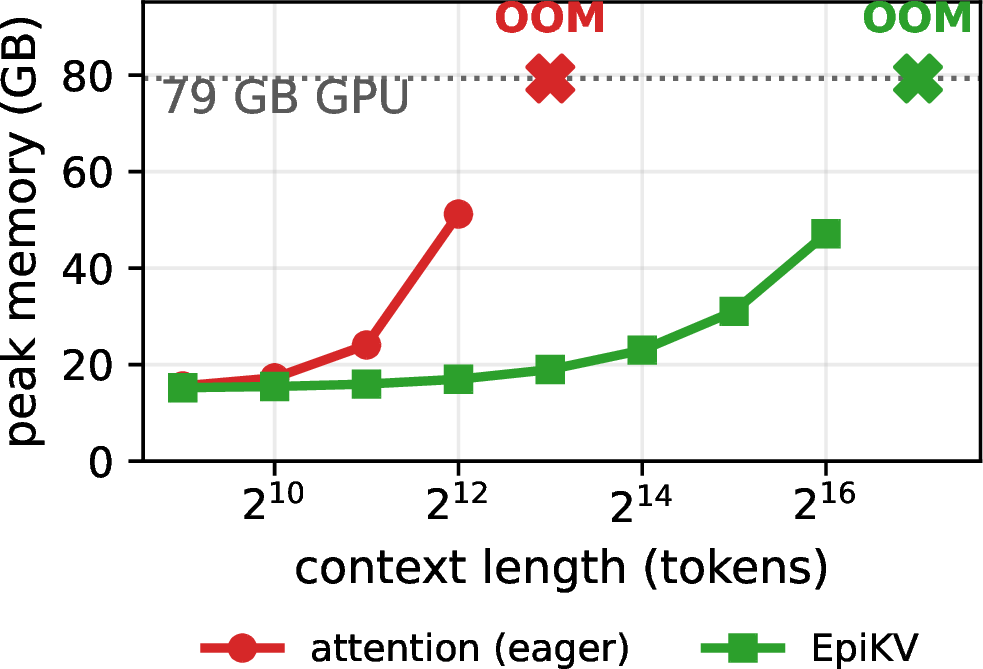
Figure 1: Peak GPU memory of a single forward pass vs.context length on an 80 GB A100. Reading attention weights (eager) grows quadratically and exhausts the GPU at 8192 tokens; the pass our method reads from scales to 65,536 – a \(16\times\) longer feasible context. This is the architectural payoff of not needing the attention matrix (detailed in §4.4)..
We introduce epiphany-aware KV cache eviction (EpiKV), which scores tokens by the change in the model’s internal representation (hidden state at specific layers and KV vectors) rather than by attention weight, and is read from the standard forward pass with no attention matrix. The name refers to the transition points in a reasoning trace (e.g., a concluded step, a committed insight) where the residual stream shifts most, which we find are the tokens worth keeping.
1.0.0.1 Contributions.
We identify a two-band layer anatomy in a 32-layer reasoning model: hidden-state change at layers 7–13 (Band A) correlates positively with token importance and at layers 18–25 (Band B) negatively, measured against counterfactual occlusion labels. The combined signal outperforms every attention-based signal we test.
We find that the raw signal carries a monotonic positional trend within a trace, as it tracks position as much as content, and we show that a causal rolling \(z\)-score removes it, recovering eviction quality.
At deployable budgets our attention-matrix-free methods match or exceed the strongest attention-based baselines on both MATH-500 and AIME-2024 (§4.3).
We quantify the engineering payoff: our method runs up to 2.8\(\times\) faster than attention-based eviction at equal budget, and avoids the attention-matrix memory wall that makes attention-based scoring infeasible at long context.
Together these make eviction deployable in standard FlashAttention serving stacks (§5.0.0.2). We release the counterfactual importance labels as a validation resource.

2 Related Work↩︎
2.0.0.1 Attention-based KV eviction.
Most eviction methods rank tokens by attention weight. H2O keeps cumulative-attention “heavy hitters” [3]; StreamingLLM keeps attention sinks plus a recent window [7]; SnapKV selects context tokens from an end-of-prompt observation window [9]; PyramidKV allocates larger budgets to lower layers [10]; and ChunkKV evicts contiguous chunks to preserve local semantics [11]. These target long inputs, and all need the attention distribution; and this requires materializing the \(n\times n\) attention matrix and so rules out the fused kernels (e.g.FlashAttention [8], [12]) that production inference relies on. We measure this cost directly (Section 4).
2.0.0.2 Reasoning-aware eviction.
A second line targets the long generation traces of reasoning models, where attention is non-monotonic and milestone tokens matter long after they are last attended. ThinKV classifies thought segments by attention sparsity and applies per-type quantization and eviction via a custom kernel [4] — needing the attention weights, an offline calibration of its sparsity thresholds and layer subset, and a token-block refresh window; RaaS uses an attention-refreshed LRU timestamp with full prefill preservation [5]; LongFlow scores by \(\lVert \mathrm{softmax}(\mathit{scores})\,V\rVert_1\) on the same model class [6]; AhaKV [13] and CAOTE [14] refine attention-based scores; and LagKV normalizes KV statistics against a lagged window, avoiding attention [15]. Except for LagKV, all derive their signal from attention. We instead use representational change in the residual stream and cached KV vectors.
2.0.0.3 Retrieval and quantization.
Orthogonal directions reduce KV cost without choosing which tokens to drop: retrieval keeps every token and fetches a subset per step [16], [17], SideQuest prompts the model to delete stale tool responses [18], and quantization lowers the precision of retained entries [19], [20]. All are stackable and complementary to our signal.
2.0.0.4 Hidden states as importance signals.
Mid-network layers carry the model’s load-bearing computation: ROME and MEMIT localise factual recall to mid-layer feed-forward modules [21], [22], which act as key–value memories [23] — the same layers (7–13) where we find the strongest positive correlation with token importance. Speculative decoding gives convergent evidence: EAGLE drafts from hidden states, not token embeddings, because they carry richer predictive structure [24].
2.0.0.5 Positioning.
No prior decode-time eviction method for reasoning traces combines a non-attention importance signal with attention-matrix-free scoring. ThinKV, RaaS, and LongFlow are reasoning-aware but attention-derived; LagKV is attention-free but generic and KV-only. Ours has both, and adds a layer-level account — a positive mid-layer of where importance lives.
3 Method↩︎
3.1 Problem setup↩︎
During autoregressive decoding the key–value (KV) cache grows by one entry per layer per generated token. For a reasoning trace of \(n\) tokens over a model with \(L\) layers and \(H\) key–value heads of dimension \(d_h\), the cache holds \(2 L H d_h n\) scalars, which for traces of \(10^4\)–\(10^5\) tokens dominates device memory. Decode-time eviction caps the cache at a budget of \(K\) tokens: at each step a policy scores the cached positions and retains the \(K\) highest-scoring ones, discarding the rest permanently.
We call a policy FlashAttention-compatible (FA2-compatible) if it computes its score using only (i) the cached keys and values, which already reside in high-bandwidth memory, and (ii) the per-layer hidden states exposed by the standard
output_hidden_states interface. Such a policy never requests output_attentions and never materializes the \(n \times n\) attention matrix, so it runs inside a FlashAttention forward pass without
forcing the eager fallback. A policy is attention-requiring if it needs the attention matrix (equivalently, output_attentions=True), which disables FlashAttention’s tiling and reintroduces \(\mathcal{O}(n^2)\) peak memory for scoring. Figure 2 contrasts the two regimes.
3.2 The hidden-state variance signal↩︎
Attention weight, the proxy used by every prior decode-time eviction method for reasoning traces, is both a noisy importance signal and architecturally costly to extract (§1); we keep these two objections separate throughout.
Our signal is the per-token change in the residual stream. For layer \(l\) and decode position \(t\), let \(h_l(t)\) be the hidden state and define the L2 diff \[g_l(t) = \lVert h_l(t) - h_l(t-1) \rVert_2 .\] A large \(g_l(t)\) indicates that generating token \(t\) shifted the model’s internal state at layer \(l\), which is the signature of a consequential token (an intermediate result, a concluded step, a transition from exploratory to convergent reasoning) rather than fluent filler. We refer to these transition points as epiphany tokens.
3.2.0.1 The two-band anatomy.
A per-layer correlation study against counterfactual importance labels (Section 3.4) identifies two bands with consistent and opposite behavior on competition mathematics. Band A (layers 7–13) has consistently positive Spearman \(\rho\): high \(g_l\) marks an important token. Band B (layers 18–25) has consistently negative \(\rho\): high \(g_l\) marks a dispensable token. We interpret the two bands in §5; the split is consistent with mid-layer factual retrieval [21]–[23]. We combine the two bands into a single score \[s(t) = \bar{g}_{10}(t) - \bar{g}_{21}(t), \label{eq:combined}\tag{1}\] where \(\bar{g}_l(t)\) is the rolling mean of \(g_l\) over the trailing window of \(w=64\) tokens. The window is causal (it uses only positions \(\le t\)), so the score for token \(t\) never depends on future tokens. Tokens with high \(s\) are retained.
3.2.0.2 The temporal-trend correction.
The raw score 1 carries a confound we discovered during analysis and report as a methodological finding. Within a single trace, \(\bar{g}_{10}\) tends to decrease and \(\bar{g}_{21}\) tends to increase with position, so \(s(t)\) tracks position as much as content: in short traces it can rank early (droppable) tokens above late (load-bearing) ones. The aggregate \(\rho\) that motivates the bands is driven partly by cross-problem structure and overstates within-trace ranking quality. We correct this with a causal rolling \(z\)-score, \[z_l(t) = \frac{g_l(t) - \mu_l(t)}{\sigma_l(t) + \varepsilon}, \label{eq:zscore}\tag{2}\] where \(\mu_l(t)\) and \(\sigma_l(t)\) are the mean and standard deviation of \(g_l\) over the trailing window, and score with \(z_{10}(t) - z_{21}(t)\). This converts absolute magnitude (position-contaminated) into local deviation (position-agnostic), in the spirit of lag-relative normalization [15] and analytical detrending [13] but applied to hidden-state diffs. The detrended variant, EpiKV, is our primary method.
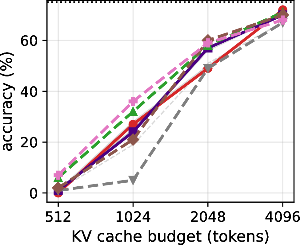
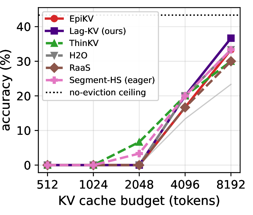
Figure 3: Accuracy vs.cache budget on MATH-500 (left, \(n{=}100\)) and AIME-2024 (right, \(n{=}30\)). Solid: FA2-compatible methods; dashed: attention-requiring; dotted: no-eviction ceiling..
3.3 Eviction policies↩︎
Table ¿tbl:tab:methods? lists every policy we evaluate. The score for each hidden-state and KV policy is computed once when a token is generated and then frozen, so scoring is fully online and causal. Each policy preserves the prompt (prefill) tokens and a trailing recency window, and applies its budget to the remaining positions.1
4pt
@llc@ Method & Signal & FA2
H2O & cumulative attention &
ThinKV & R/E/T segment entropy &
RaaS & attention LRU timestamp &
HS-variance & \(\bar{g}_{10}-\bar{g}_{21}\) &
& \(z_{10}-z_{21}\) &
Band-adaptive & Band A/B layers &
KV-key var & key variance &
KV-val var & value variance &
Lag-KV & lag-norm.key\(+\)value &
Attn\(\times\)HS & cumul.attn \(+\,z_{10}\) &
Segment-HS & ThinKV seg.\(+\) HS rank &
The KV-vector family scores tokens from quantities already in the cache, with no hidden states required. KV-key and KV-val use the rolling-mean variance of the key and value vectors across head dimension. Lag-KV adapts the lag-relative normalization of [15] to streaming decode: each token’s key and value vectors are normalized by the previous chunk’s per-channel range before the variance is taken, which removes domain-level magnitude shifts. We use the previous chunk (causal) rather than the next chunk (look-ahead) used by the original prefill-time formulation.
3.4 Counterfactual importance labels↩︎
The band anatomy rests on ground-truth importance labels obtained by counterfactual occlusion (full protocol in Appendix 8). For each correctly answered trace we slide a 32-token window (stride 16) over the reasoning span, replace it with padding, regenerate the answer from the modified context, and label the window important if the answer changes (logical-OR over overlapping windows). The occlusion feeds the same context length for every window, so the label measures content, not position — unlike an earlier truncation variant that proxied position and inflated attention signals. Regeneration is greedy. The important fraction is \(\approx\)0.20 on MATH-500 and 0.52–0.64 on AIME, reflecting that nearly every token of a hard problem is load-bearing.
3.5 Experimental setup↩︎
3.5.0.1 Model.
DeepSeek-R1-Distill-LLaMA-8B (32 layers) [1], chosen for direct comparability with ThinKV and for being an open-weight member of the reasoning-model class. Generation is greedy throughout, so reported differences are not sampling noise.
3.5.0.2 Datasets.
MATH-500 [25], [26] is primary benchmark (competition maths, verifiable boxed answers, traces of \(\sim\)4k–16k tokens). AIME-2024 tests higher cache pressure with \(\sim\)16k–32k-token traces. GSM8K [27] is used only as a difficulty-regime probe for the layer anatomy (App. 11), not as a head-to-head accuracy benchmark.
3.5.0.3 Budgets and metrics.
Cache budgets \(K \in \{512, 1024, 2048, 4096\}\) on MATH-500 and \(\{512,\dots,8192\}\) on AIME-2024. We report accuracy (exact match on the boxed answer), per-problem wall-clock time, and per-example peak GPU memory (reset before each problem).
3.5.0.4 Attention back-end.
Attention-requiring policies run in eager mode; FA2-compatible ones with flash_attention_2, as a separate configuration (unaffected by the back-end since they never read the attention matrix). Each run uses one GPU of our cluster’s
comparable 46–49 GB cards (L40, L40S, RTX 6000 Ada, A6000); see Appendix 13.
4 Results↩︎
We report the H2O failure that motivates a non-attention signal (§4.1), the signal validation behind the two-band anatomy (§4.2), end-to-end accuracy at each budget (§4.3), the speed and memory profile (§4.4), and the difficulty-regime anatomy (§4.5). Full tables are in Appendix 7.
4.1 Attention-based eviction collapses↩︎
H2O does not degrade gracefully on reasoning traces; it collapses. On MATH-500 its accuracy falls from 67% at a 4096-token budget to 49% at 2048 and 5% at 1024 (Table 2), an order of magnitude below the no-eviction ceiling of 75%. The collapse is empty output rather than wrong output: H2O produces no generated answer on 93 of 100 problems at a 1024-token budget, 48 at 2048, and 27 at 4096 (immediate end-of-sequence); at 512 it instead emits unstructured text with no extractable answer on 99 of 100. This matches the attention-map failure RaaS documents on reasoning traces, and is the empirical case for not deriving the eviction signal from attention.
4.2 The two-band importance signal↩︎
The two-band anatomy of §3.2 (Band A positive, Band B negative) holds against the occlusion labels consistently across both competition-mathematics datasets and both attention back-ends (Appendix 6). Cumulative attention (h2o_attn) is the weakest signal measured, with \(|\rho|\le 0.09\) on every eager dataset, below every hidden-state band layer. A causal rolling-64 window
improves correlation over the raw signal by 32–57% across datasets (Table 9); pre-RoPE key statistics give no measurable benefit (\(\Delta|\rho|\le 0.0005\)).
4.3 Accuracy at deployable budgets↩︎
At a 4096-token cache on MATH-500, EpiKVreaches 72%, above ThinKV (71%) and H2O (67%) and within 3 points of the 75% ceiling (Table 2; Figure 3); the FA2-compatible family clusters at 70–72% while the attention-requiring baselines span 67–71%. The margin over the best attention baseline is one problem of 100, so we claim parity-or-better at this budget; and we obtain it without ever materializing the attention matrix. On AIME-2024 at 8192 the lag-normalized KV method reaches 37% against 33% for the best attention-requiring method (Table 3); at \(n{=}30\) this is one problem of difference.
Two honest qualifications. First, no single FA2-compatible method dominates across budgets: at 2048 on MATH-500 the band-adaptive and KV variants reach 57% while EpiKVdrops to 49%, and RaaS leads at 60%. Second, at the tightest budgets (\(\le\)1024) an eager hybrid that combines segment classification with the hidden-state ranker leads (36% at 1024, 7% at 512), and no FA2-compatible method matches it there. The contribution here is parity-or-better with attention-based eviction at the budgets that matter for deployment, obtained without materializing the attention matrix.
4.4 Speed and memory↩︎
4.4.0.1 Speed.
Two effects make eviction faster. First, a capped cache shrinks per-step attention, so every eviction method (even eager ones) runs below the uncapped no-eviction baseline (763 s on AIME-2024 at 8192). Second, FA2-compatible methods additionally avoid the eager-attention kernel: on AIME-2024 at 8192 the lag-normalized method (440 s per problem) is 1.6\(\times\) faster than ThinKV, the fastest attention baseline (721 s), and up to 2.8\(\times\) faster overall (RaaS, 1239 s; Table 5, Figure 4). This FA2 speed-up is method-specific, not automatic — the raw key-variance and lag-key variants recompute scores over the whole cache each step and only match the eager baselines — and H2O’s low wall-time at tight budgets reflects its empty-generation collapse, not efficiency.
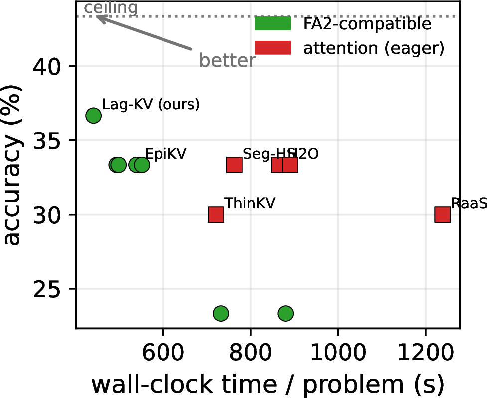
Figure 4: Accuracy vs.wall-clock time per problem on AIME-2024 at an 8192-token budget — top-left is better. FA2-compatible methods (green) dominate the accuracy–speed frontier; Lag-KV is both the most accurate and the fastest, while the attention-based baselines (red) sit slower and no more accurate..
4.4.0.2 Memory.
In the decode regime measured, peak memory is set by the cache budget, not the method: at the tightest AIME budget every eviction method saves \(\approx\)2.9 GB over no eviction (Table 7).
The architectural memory advantage of being FA2-compatible appears at prefill, where reading attention weights materializes the \(H{\times}n{\times}n\) maps. On an 80 GB A100, a forward pass with
output_attentions=True already uses 52 GB at a 4096-token context and runs out of memory at 8192 whereas a FlashAttention pass over the same model scales to 65,536 tokens at 48 GB, a 16\(\times\) longer
feasible context (Figure 1). This compounds at the batch level: holding the cache at a 2048-token budget supports 224 concurrent 32,768-token requests on the same GPU against 14 without eviction (App. 14), and the gap widens with context length.
4.5 Difficulty-regime anatomy↩︎
The two-band anatomy is specific to competition mathematics. On GSM8K (grade-school arithmetic, \(n_{\mathrm{eff}}{=}352\)) the positive band moves to early layers and the negative band extends across most of the network, and both attention entropy and key variance reverse sign relative to MATH-500 (Appendix 11). Where the importance signal lives depends on task difficulty, and this is evidence that the signal tracks a real property of how reasoning is consolidated, not a fixed layer index.
5 Discussion↩︎
5.0.0.1 What the two-band anatomy means, and why it moves.
The positive band (layers 7–13) coincides with the mid-network layers that mechanistic-interpretability work identifies as the site of factual retrieval and feature routing [21]–[23]: large hidden-state change there marks a token where the model retrieves or composes content. The negative band (18–25) is the counterintuitive half: these upper-mid layers prepare the output distribution and are active even for fluent, low-surprise tokens, so large change there signals predictable continuation rather than content worth keeping; subtracting the bands exploits this opposition. The band locations are not universal — they shift with task difficulty (§4.5, Appendix 11) — which indicates the signal tracks where load-bearing computation happens (deeper for harder problems) and makes the layer indices a per-regime hyperparameter (layers 10 and 21 for the competition-mathematics setting we target).
5.0.0.2 Attention-matrix-free scoring is the deployment contribution.
No prior decode-time eviction method for reasoning traces avoids the attention matrix: ThinKV needs the attention weights, an offline calibration step, and a custom kernel, and H2O, RaaS, and LongFlow all require the attention weights and therefore the eager kernel. The cost of that requirement is not academic. At the 16k–64k contexts typical of reasoning traces, reading the attention weights to score tokens exhausts GPU memory before the trace even fits (§4.4), while our signal is read from the same forward pass the model already runs. Scoring is also causal: the rolling \(z\)-score fixes a token’s fate at the step it is produced, where ThinKV’s \(\tau{=}128\) refresh window defers classification by up to \(\tau\) tokens. EpiKV drops into vLLM, TGI, or SGLang unchanged, with no training, no classifier, and no kernel fork. For a method already at accuracy parity and faster at equal budget, that is what makes it well-suited to production.
5.0.0.3 A trend that residual-stream signals share.
The finding that the raw hidden-state signal carries a monotonic positional trend within a trace — so that aggregate correlation overstates within-trace ranking quality — is not specific to our method. Any importance signal read from the residual stream over a long generation is exposed to the same drift, and the causal rolling \(z\)-score we use is a cheap, general correction. The deeper cause, that certain layers have systematically different activation magnitudes early versus late in a generation, is worth study in its own right.
5.0.0.4 Limitations.
Latency and memory are measured single-GPU and single-example; batched and multi-GPU throughput is projected from KV-cache arithmetic (Appendix 14) rather than measured end-to-end, and the prefill-memory advantage is shown by a forward-pass microbenchmark, not a long-prompt deployment. The AIME-2024 comparison is \(n{=}30\), where a three-point gap is a single problem (Appendix 12); pooling AIME 2024–2026 to \(n{\approx}90\) would firm it up. Results are from one model family (DeepSeek-R1-Distill-LLaMA-8B), as is common in this line of work; transfer across architectures and scales is untested.
5.0.0.5 Futubibliographystylere work.
As extensions, an attention-matrix-free analogue of the segment hybrid (e.g., segment classification from KV statistics rather than attention entropy) would target the tight-budget regime where the eager hybrid still leads. Chunk-level scoring [11] over hidden-state change and per-layer budgets [10] are orthogonal gains, and quantization [19], [20] is stackable.
Acknowledgements↩︎
We thank Vashisth Tiwari for their helpful comments and pointers in the ideation of this work.
6 Per-layer importance correlations↩︎
Table 1 reports the Spearman \(\rho\) between \(\bar{g}_l\) (rolling-64 hidden-state L2 diff at layer \(l\)) and the counterfactual importance labels, for all 32 layers on the two competition-mathematics datasets in both attention back-ends. Band A (7–13) is positive throughout; Band B (18–25) is negative throughout. The last layer (l31) flips sign across datasets and is not used.
| \(l\) | math500 | m500-eag | aime24 | aime24-eag |
|---|---|---|---|---|
| 0 | \(-\)0.173 | \(-\)0.199 | \(-\)0.068 | \(+\)0.037 |
| 1 | \(-\)0.172 | \(-\)0.202 | \(-\)0.089 | \(-\)0.052 |
| 2 | \(-\)0.121 | \(-\)0.151 | \(-\)0.101 | \(-\)0.125 |
| 3 | \(-\)0.121 | \(-\)0.124 | \(-\)0.014 | \(-\)0.072 |
| 4 | \(-\)0.153 | \(-\)0.139 | \(+\)0.011 | \(-\)0.052 |
| 5 | \(-\)0.079 | \(-\)0.058 | \(+\)0.083 | \(+\)0.093 |
| 6 | \(+\)0.011 | \(-\)0.007 | \(+\)0.120 | \(+\)0.150 |
| 7 | \(+\)0.079 | \(+\)0.047 | \(+\)0.118 | \(+\)0.156 |
| 8 | \(+\)0.065 | \(+\)0.078 | \(+\)0.146 | \(+\)0.155 |
| 9 | \(+\)0.082 | \(+\)0.107 | \(+\)0.136 | \(+\)0.130 |
| 10 | \(+\)0.112 | \(+\)0.141 | \(+\)0.097 | \(+\)0.120 |
| 11 | \(+\)0.093 | \(+\)0.144 | \(+\)0.083 | \(+\)0.120 |
| 12 | \(+\)0.038 | \(+\)0.077 | \(+\)0.119 | \(+\)0.114 |
| 13 | \(+\)0.071 | \(+\)0.089 | \(+\)0.058 | \(+\)0.065 |
| 14 | \(-\)0.016 | \(+\)0.006 | \(-\)0.020 | \(-\)0.032 |
| 15 | \(+\)0.017 | \(+\)0.016 | \(-\)0.124 | \(-\)0.147 |
| 16 | \(-\)0.002 | \(-\)0.016 | \(-\)0.140 | \(-\)0.165 |
| 17 | \(-\)0.003 | \(-\)0.005 | \(-\)0.147 | \(-\)0.191 |
| 18 | \(-\)0.081 | \(-\)0.045 | \(-\)0.118 | \(-\)0.184 |
| 19 | \(-\)0.147 | \(-\)0.074 | \(-\)0.113 | \(-\)0.208 |
| 20 | \(-\)0.191 | \(-\)0.097 | \(-\)0.105 | \(-\)0.224 |
| 21 | \(-\)0.209 | \(-\)0.109 | \(-\)0.085 | \(-\)0.227 |
| 22 | \(-\)0.223 | \(-\)0.121 | \(-\)0.059 | \(-\)0.217 |
| 23 | \(-\)0.254 | \(-\)0.151 | \(-\)0.021 | \(-\)0.200 |
| 24 | \(-\)0.250 | \(-\)0.146 | \(-\)0.005 | \(-\)0.188 |
| 25 | \(-\)0.243 | \(-\)0.142 | \(-\)0.006 | \(-\)0.187 |
| 26 | \(-\)0.211 | \(-\)0.107 | \(+\)0.007 | \(-\)0.157 |
| 27 | \(-\)0.066 | \(-\)0.003 | \(-\)0.041 | \(-\)0.086 |
| 28 | \(-\)0.053 | \(-\)0.018 | \(-\)0.041 | \(-\)0.059 |
| 29 | \(+\)0.082 | \(+\)0.049 | \(-\)0.099 | \(+\)0.030 |
| 30 | \(+\)0.135 | \(+\)0.065 | \(-\)0.121 | \(+\)0.062 |
| 31 | \(+\)0.220 | \(+\)0.093 | \(-\)0.178 | \(-\)0.022 |
4pt
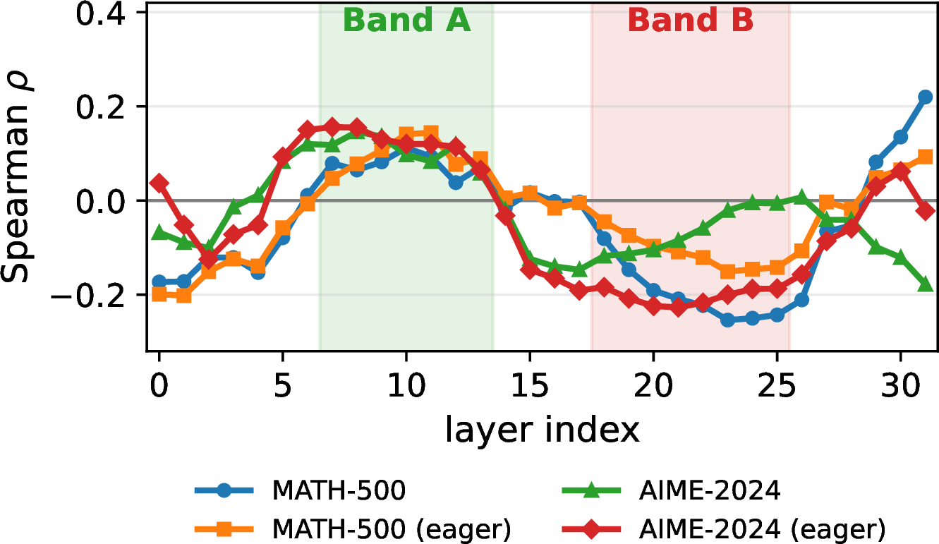
Figure 5: Per-layer Spearman \(\rho\) between rolling-64 hidden-state change and counterfactual importance. Band A (7–13) is positive and Band B (18–25) negative across both datasets and back-ends..
7 Full Phase 1 results↩︎
Tables 2–7 give the complete accuracy, per-problem wall-clock time, and per-example peak GPU memory for every method and budget. FA2-compatible methods are marked . MATH-500 is \(n{=}100\); AIME-2024 is \(n{=}30\) (each problem \(\approx\)3.3 points).
| Method | FA2 | 512 | 1024 | 2048 | 4096 |
|---|---|---|---|---|---|
| none | 75.0 | ||||
| 0.0 | 27.0 | 49.0 | 72.0 | ||
| hs-variance | 1.0 | 28.0 | 50.0 | 71.0 | |
| band-adaptive | 1.0 | 25.0 | 57.0 | 70.0 | |
| kv-val | 1.0 | 24.0 | 56.0 | 70.0 | |
| kv-key | 1.0 | 24.0 | 57.0 | 70.0 | |
| lag-kv-key | 1.0 | 25.0 | 57.0 | 70.0 | |
| lag-kv | 1.0 | 24.0 | 57.0 | 70.0 | |
| thinKV | 6.0 | 32.0 | 58.0 | 71.0 | |
| h2o | 1.0 | 5.0 | 49.0 | 67.0 | |
| raas | 2.0 | 21.0 | 60.0 | 70.0 | |
| hybrid-seg-hs | 7.0 | 36.0 | 59.0 | 68.0 | |
| attn\(\times\)hs | 1.0 | 19.0 | 51.0 | 67.0 | |
4pt
| Method | FA2 | 512 | 1024 | 2048 | 4096 | 8192 |
|---|---|---|---|---|---|---|
| none | 43.3 | |||||
| 0.0 | 0.0 | 0.0 | 16.7 | 33.3 | ||
| hs-variance | 0.0 | 0.0 | 0.0 | 16.7 | 33.3 | |
| band-adaptive | 0.0 | 0.0 | 0.0 | 16.7 | 33.3 | |
| kv-val | 0.0 | 0.0 | 0.0 | 16.7 | 33.3 | |
| kv-key | 0.0 | 0.0 | 0.0 | 13.3 | 23.3 | |
| lag-kv-key | 0.0 | 0.0 | 0.0 | 13.3 | 23.3 | |
| lag-kv | 0.0 | 0.0 | 0.0 | 20.0 | 36.7 | |
| thinKV | 0.0 | 0.0 | 6.7 | 20.0 | 30.0 | |
| h2o | 0.0 | 0.0 | 0.0 | 20.0 | 33.3 | |
| raas | 0.0 | 0.0 | 0.0 | 16.7 | 30.0 | |
| hybrid-seg-hs | 0.0 | 0.0 | 3.3 | 20.0 | 33.3 | |
| attn\(\times\)hs | 0.0 | 0.0 | 0.0 | 20.0 | 33.3 | |
3.5pt
| Method | 512 | 1024 | 2048 | 4096 |
|---|---|---|---|---|
| none | \(\approx\)180 | |||
| 319.9 | 276.9 | 181.9 | 125.0 | |
| hs-variance | 342.1 | 282.2 | 181.9 | 128.8 |
| band-adaptive | 272.4 | 246.3 | 155.3 | 113.8 |
| kv-val | 271.5 | 249.4 | 152.5 | 113.5 |
| kv-key | 273.5 | 248.7 | 156.0 | 113.4 |
| lag-kv-key | 269.1 | 251.0 | 158.3 | 116.3 |
| lag-kv | 267.5 | 252.0 | 163.4 | 119.5 |
| thinKV | 520.2 | 416.5 | 399.4 | 344.6 |
| h2o | 628.0 | 40.2 | 71.4 | 91.4 |
| raas | 873.3 | 515.8 | 317.8 | 246.6 |
| hybrid-seg-hs | 420.9 | 309.2 | 222.5 | 193.8 |
| attn\(\times\)hs | 572.1 | 414.4 | 290.5 | 211.5 |
4pt
| Method | 512 | 1024 | 2048 | 4096 | 8192 |
|---|---|---|---|---|---|
| none | \(\approx\)762 | ||||
| 630.1 | 601.3 | 614.8 | 565.0 | 538.5 | |
| hs-variance | 617.5 | 604.3 | 615.3 | 561.7 | 551.1 |
| band-adaptive | 547.4 | 551.1 | 556.1 | 521.6 | 493.3 |
| kv-val | 547.9 | 553.1 | 560.4 | 523.9 | 497.7 |
| kv-key | 893.8 | 891.5 | 884.6 | 782.9 | 732.1 |
| lag-kv-key | 874.4 | 974.9 | 998.3 | 913.8 | 879.7 |
| lag-kv | 1013.6 | 505.0 | 533.0 | 499.7 | 440.5 |
| thinKV | 849.0 | 788.1 | 770.5 | 746.5 | 721.0 |
| h2o | 963.2 | 981.1 | 1007.0 | 865.7 | 864.5 |
| raas | 885.2 | 899.2 | 921.6 | 1285.2 | 1238.7 |
| hybrid-seg-hs | 944.2 | 927.8 | 933.9 | 783.2 | 763.0 |
| attn\(\times\)hs | 1327.5 | 1352.5 | 1021.2 | 884.9 | 889.8 |
3.5pt
| Method | 512 | 1024 | 2048 | 4096 |
|---|---|---|---|---|
| none | 16221 | |||
| 15525 | 15692 | 15880 | 16063 | |
| band-adaptive | 15525 | 15698 | 15880 | 16064 |
| kv-key | 15525 | 15697 | 15880 | 16064 |
| lag-kv | 15524 | 15697 | 15880 | 16064 |
| thinKV | 15508 | 15643 | 15836 | 16036 |
| h2o | 15560 | 15574 | 15714 | 15814 |
| raas | 15560 | 15743 | 15933 | 16136 |
| hybrid-seg-hs | 15525 | 15655 | 15857 | 16065 |
| attn\(\times\)hs | 15568 | 15747 | 15968 | 16201 |
4pt
| Method | 512 | 1024 | 2048 | 4096 | 8192 |
|---|---|---|---|---|---|
| none | 18448 | ||||
| 15526 | 15712 | 16097 | 16791 | 17918 | |
| kv-key | 15525 | 15712 | 16097 | 16781 | 17919 |
| lag-kv | 15524 | 15712 | 16097 | 16750 | 17647 |
| thinKV | 15521 | 15653 | 15953 | 16489 | 17374 |
| h2o | 15567 | 15759 | 16170 | 16840 | 17946 |
| raas | 15567 | 15759 | 16170 | 16900 | 18087 |
| hybrid-seg-hs | 15550 | 15672 | 15976 | 16485 | 17334 |
| attn\(\times\)hs | 15584 | 15764 | 16173 | 16841 | 17946 |
3.5pt
8 Counterfactual labeling details↩︎
Labels are produced by sliding-window occlusion over the reasoning span of each correctly answered trace. Window size 32, stride 16 (each interior position is covered by two windows). The answer boundary is located by searching for the
</think> token sequence, falling back to the last \ boxed{ and then to the final 64 tokens. For each window the tokens are replaced with the padding id, the full modified context up to the boundary is fed, and the answer is
regenerated greedily with up to 512 new tokens. A position is labeled important (1) if any covering window flips the answer, else 0; prompt positions are fixed to 1 and the answer span is not tested. Regeneration is deterministic, so labels are
reproducible.
9 Eviction policy composition and budgets↩︎
Table 8 records, for each method, which structural tokens are preserved and how the budget \(K\) is allocated. The policies differ: H2O preserves sinks plus a recency window, RaaS and the hidden-state/KV families preserve the entire prefill, and ThinKV preserves only a recency window and may retain fewer than \(K\) tokens because its per-segment R/E/T budgets (\(\{64,32,8\}\)) need not sum to \(K\). Recency is \(\min(128, K/4)\) throughout.
| Method | Always kept | Budget rule | \(\le K\) |
|---|---|---|---|
| H2O | 4 sinks \(+\) recency | top cumul.attn | \(=K\) |
| ThinKV | recency | R/E/T per seg. | \(\le K\) |
| RaaS | all prefill | LRU on decode | \(=K\) |
| HS family | all prefill \(+\) rec. | top \(s(t)\)/\(z\) | \(=K\) |
| KV/Lag | all prefill \(+\) rec. | top variance | \(=K\) |
3pt
10 Temporal smoothing and RoPE↩︎
Rolling-64 smoothing outperforms an EMA (\(\alpha{=}0.9\)) and the raw signal across datasets (Table 9). Pre-RoPE versus post-RoPE key statistics is a null result: the maximum \(\Delta|\rho|\) observed across datasets and smoothing variants is 0.0005, so pre-RoPE collection is omitted.
| Dataset | raw | EMA | rolling-64 |
|---|---|---|---|
| math500 | 0.288 | 0.356 | 0.380 |
| math500-eager | 0.150 | 0.193 | 0.214 |
| aime2024 | 0.139 | 0.183 | 0.203 |
| aime2024-eager | 0.014 | 0.018 | 0.022 |
11 GSM8K difficulty-regime anatomy↩︎
On GSM8K (355 correctly answered traces, \(n_{\mathrm{eff}}{=}352\)) the layer anatomy shifts relative to competition mathematics. Band A moves to early layers (l0–l7 positive; l0 \(=+0.181\)), the negative band extends across l10–l30 (strongest l15 \(=-0.351\)), and the last layer is strongly positive (l31 \(=+0.231\)). Attention entropy reverses sign relative to MATH-500 (\(-0.313\) vs.\(+0.176\)) and kv-key variance reverses (\(-0.261\) vs.\(+0.380\)); both reversals are confirmed at high \(n_{\mathrm{eff}}\). The shift indicates that where the importance signal lives depends on task difficulty: harder problems route load-bearing computation through mid-layers, simpler arithmetic through early layers. GSM8K is therefore reported as a difficulty-regime probe, not a head-to-head accuracy benchmark.
12 Statistical power↩︎
Effective sample size is the number of independent traces, not token pairs, since tokens within a trace are correlated. Table 10 gives \(n_{\mathrm{eff}}\) and the approximate 95% confidence half-width (Fisher \(z\)). MATH-500 and GSM8K are the only high-power datasets; every AIME configuration has a confidence interval spanning zero, which is why AIME results are reported as directional and tagged for pooling to \(n{\approx}90\).
| Dataset | \(n_{\mathrm{eff}}\) | \(\pm\)SE (\(\rho\)) |
|---|---|---|
| math500 | 72 | 0.118 |
| math500-eager | 78 | 0.113 |
| gsm8k-eager | 352 | 0.053 |
| aime2024 | 11 | 0.301 |
| aime2024-eager | 8 | 0.354 |
| aime2025/2026 | \(\le 5\) | \(\ge 0.45\) |
13 Implementation notes↩︎
Eviction is applied through the HuggingFace DynamicCache. Two issues required fixes for correctness: keep-masks were moved to each tensor’s device for multi-GPU device_map="auto" runs, and the post-eviction cache is rebuilt by
constructing an empty DynamicCache and calling update per layer so that _seen_tokens matches the retained length (otherwise the model builds a causal mask one position too long). Multi-GPU FlashAttention runs hit a
kernel-coordination launch failure, so all flash benchmarks use a single GPU. The no-eviction baseline is run once and copied across budgets. The prefill-memory microbenchmark (Section 4) was run on an NVIDIA A100
(80 GB). The Phase-1 accuracy/time/memory benchmarks ran on the cluster’s comparable 46–49 GB GPUs (NVIDIA L40, L40S, RTX 6000 Ada, RTX A6000), one GPU per job.
14 Throughput projection↩︎
Figure 6 projects the maximum number of concurrent requests that fit on an 80 GB GPU as a function of context length, computed from the per-token KV-cache size, with and without eviction.
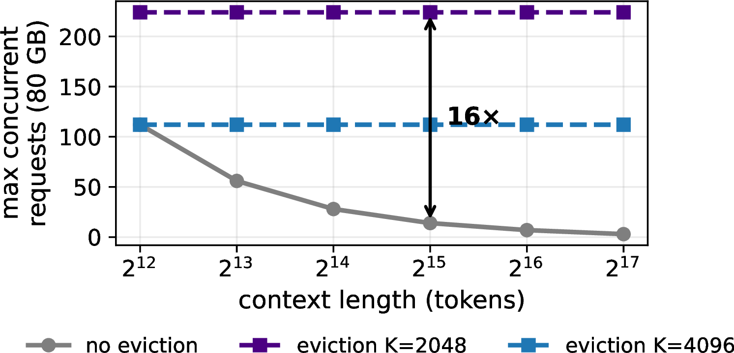
Figure 6: Maximum concurrent requests on an 80 GB GPU vs.context length. Without eviction, capacity falls as traces grow; a fixed cache budget holds it flat..