auto-psych: Automating the science of mind using agent-driven theory discovery and experimentation
June 24, 2026
Abstract
AI-based scientific automation is increasingly possible by using agents to generate hypotheses, design experiments, and analyze data. Data collection is a major bottleneck in this pipeline, however. Psychology, and computational cognitive science in particular, is well-positioned to benefit from AI experimentation because theories are often represented as code and crowdsourcing platforms enable programmatic human data collection at scale. Here, we apply automated discovery techniques to the project of generating theories in computational cognitive science, with an agent-based system collecting human data independently through crowdsourced survey experiments. As a testbed, we use a classic case study from cognitive psychology: judging which sequences of coin flips seem subjectively more random. Our system, auto-psych, uses nested agent-based discovery loops to generate explanatory theories of human behavior. The inner loop conjectures, fits, and critiques probabilistic cognitive models; the outer loop designs experiments to test these models, launches them online, and analyzes the data. This system can quickly and reliably recover ground-truth theories from synthetic data via systematic experimentation, but the nested structure is critical to model performance. Further, in three independent sequences of human experiments, the system finds theories that fit the data better than theories generated from the scientific literature. This work thus demonstrates the feasibility of automated data collection and theory discovery in computational cognitive science.
1 Introduction↩︎
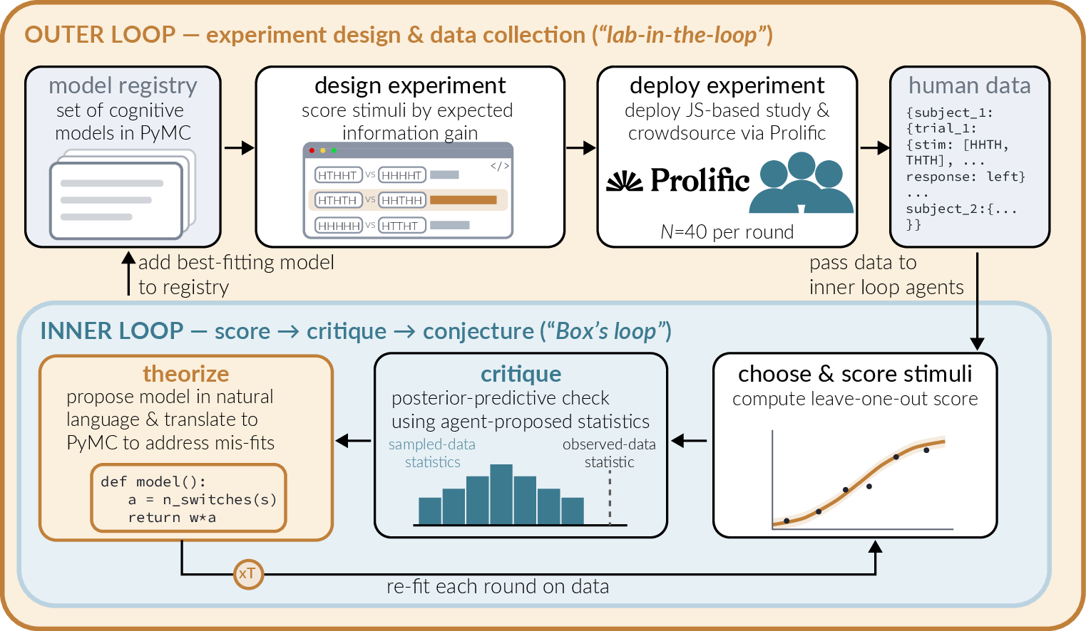
The scientific process is often described as an iterative loop in which researchers conjecture a theory, devise specific experimental tests of that theory, and then adjust their theory in response to evidence [1].1 AI tools can already assist with each step in this loop – helping to create theories, design experiments, and analyze and interpret data [3]–[9]. Could AI systems complete every part of the discovery loop? Such an advance could lead to increasing automation of the scientific process and faster progress towards important applications [4], [10]. Agent-based systems built on large language models can now use computational tools and integrate with data collection platforms, making this goal increasingly feasible. As a step towards it, the current paper develops a framework that automates the complete model discovery loop in computational cognitive science.
Recent progress has been made in developing language model-based workflows across the sciences, but these projects have focused on model discovery from existing datasets. The pattern of iterative model testing and refinement on a known dataset is sometimes known as “Box’s loop” (after statistician George Box) [11]. Because no new data are needed, language model agents can quickly propose, fit, and critique models [7], [9], [12]. However, a critical part of the scientific process is collecting new data under targeted experimental regimes to test theories. Thus, current AI-driven science requires a “lab-in-the-loop” model [13], [14], which limits the speed of iteration because of the need for scientists to carry out the experiments.
End-to-end scientific automation has been a major goal in machine learning research, where AI agents can run experiments without humans in the loop. For example, one automated system for computational research decomposes each problem into a set of steps – idea generation, novelty checking, experimentation, and paper writing [15]; parallel passes through this workflow with comparison and pruning at each step resulted in an agent-generated paper that passed human review [16]. Even for in silico systems, reducing data collection bottlenecks is critical to rapid iteration [17].
Experimentation in psychology requires human participants, but many studies are run online via crowdsourcing platforms like Amazon Mechanical Turk and Prolific [18], [19]. Such experiments are typically served in template-based web frameworks [20], meaning that they can be created by artificial agents and deployed via application programming interfaces (APIs). Just as autonomous machine learning research depends on small-scale training runs, autonomous psychology can make use of fast and inexpensive online behavioral experiments.
Computational cognitive science is a sub-field of psychology that might have the most to gain from automated experimentation. Extensive work has been done to formalize theories in this domain. In particular, probabilistic models in the Bayesian tradition provide a unifying language for describing contentful hypotheses about the mind [21]. These theories can be expressed in a number of highly expressive and well-documented probabilistic programming languages (e.g., Stan, PyMC, Pyro) [22]–[25], meaning that they can be generated by coding agents and compared with one another using standard statistical approaches. While previous work has automatically generated and compared cognitive models of this type [26], their workflows have yet to be integrated into a full human experimentation loop.
In the current paper, we implement an automated theory discovery and experimentation loop for computational cognitive science (Figure 1), which we call auto-psych. We start with a simple testbed: a well-studied problem in the psychology literature – what makes a sequence of coin flips appear more or less random [27]–[31]. Subjective randomness is a compelling psychological problem because we have strong intuitions that, say, HTHTHTHT is a less random sequence than HTTHHHTH, despite the two being equiprobable for a fair coin. Using this problem as our case study, we develop an agent-based scientific discovery framework for creating computational theories. The core of this system is two nested loops: an outer loop that proposes probabilistic cognitive models, designs online experiments, and collects and analyzes data (the “lab-in-the-loop”), and an inner loop that critiques cognitive models and iteratively refines them (Box’s loop).
We show that our system reliably recovers ground-truth models (behavioral proxies) through iterative experimentation. We then let our agents run chains of experiments on human participants, finding strong theory discovery. In the discussion, we reflect on the promise of this system as well as potential downsides of autonomous scientific agents.
2 Related work↩︎
Much recent development has focused on autonomous computational discovery, distinguishing single-agent systems [17], [32] from multi-agent systems that coordinate ensembles of agents with different roles [13], [33] (an approach that we follow here). Work in both of these traditions has developed methods for automatically generating, critiquing, and revising statistical models [7], [12], [34], [35] as well as benchmarking their experiment planning abilities [36].
Similar approaches have yielded positive results in structural biology, helping predict protein structures and biochemical interactions on par with in vitro experimentation, enabling the rapid development of novel theories [6], [13], [14], [37]–[40]. Agent-based workflows have found solutions to open problems and proposed new algorithms in mathematics [3], [41], [42], and have been applied successfully to the social sciences and cognitive science [4], [26], [34], [43], [44]. Of this work, [26] is closest to our work as they use AI models as part of a pipeline to propose and validate probabilistic cognitive models. However, none of these works has sought to automate the entire process of computational cognitive science, from conjecturing and evaluating hypotheses to designing and running experiments with real human participants.
Our specific work here focuses on subjective randomness – people’s perception and judgments of how random a given sequence of events is. A substantial literature has considered heuristics that people might use [27], [28]. Popular accounts include representativeness of a prototype [29], algorithmic complexity [45], [46], Bayesian inference accounts [30], [31], and accounts that appeal to a finite attentional window [47].
3 Methods↩︎
Our framework uses LLM-based agents in coding harnesses to instantiate two loops: an inner loop that conjectures, fits, and critiques models and an outer loop that designs and runs experiments. Both loops use the OpenCode harness with gemini-3.1-pro-preview as the language model. We begin by describing the subjective randomness domain, then turn to the details of the workflow. Code and data are available on GitHub. Further methodological details can be found in Appendix 6.
3.1 Subjective randomness↩︎
The primary question in studies of subjective randomness is which sequences of coin flips are perceived to be more random. For purposes of our study, we choose a simple forced-choice paradigm in which participants are presented with two sequences and asked to choose between them. This setting has many desirable properties for automatically generating and testing cognitive models: the space of possible stimuli is discrete and tractable to enumerate, the experimental paradigm is straightforward, and models need only generate a probability to be assigned to each sequence.
To seed our loop with models from the literature, we added four models: 1) an “encoding compressibility” model that uses heuristic features like periodicity and long runs as proxies for the compressibility of a sequence [45], 2) a simplified version of a “Bayesian diagnosticity” account that approximates the log-likelihood ratio that a sequence was generated by a fair coin compared to a more regular computational process [30], [31], 3) a “window typicality” model inspired by [47] that judges a sequence based on whether its longest run is typical of a fair coin viewed through a finite memory window, and 4) a “prototype similarity” model that judges sequences’ randomness based on how well their heads/tails imbalance and alternation rate resemble a mental prototype [29], [48]. These models are not identical to the versions developed in the original papers, but they adapt the key ideas from these accounts of subjective randomness judgments.
3.2 Theory framework↩︎
In our framework, a cognitive model is instantiated as a probabilistic program: snippets of Python code written in the PyMC framework [49]. Each program defines a distribution over participant choices as a function of key stimulus properties, for example a sequence’s length, the number of observed Hs, or how often the sequence alternates between H and T. Each model also contains a choice-sensitivity parameter that helps determine how strongly a difference in perceived randomness maps to participant response choices and typically includes a bias parameter that captures a left vs. right response bias. We place weak priors over these free parameters and infer distributions by fitting the models to observed data.
3.3 Modeling loop↩︎
The auto-psych workflow consists of two loops: an outer loop that adds new theories, chooses stimuli that optimally distinguish between models, and implements experiments. In the first iteration, auto-psych is initialized with a set of seed models. In subsequent iterations, a theorist agent comes up with at least one new theory in a manner inspired by the “hypothesis search” framework: the agent first writes a theory in natural language, then translates it to PyMC code [50]. The theorist’s models are added to the registry of models to be compared. Next, a design agent generates 100 to 300 candidate stimuli for the experiment and scores them by their expected information gain (EIG) with respect to the models under consideration [9], [51], [52]. We compute EIG using a uniform prior over models in the registry on each step. After choosing stimuli, an implementation agent writes an experiment using jsPsych. We gave the agent a strict template to follow and automatically added our consent form to the experiment code. The agent deploys the experiment to Firebase and recruits participants using the Prolific API. It then polls the Prolific study to monitor when it is completed, pulls the data, and continues the loop. All experiments were approved under Stanford IRB protocol #20009. More details about the human experiments can be found in Appendix 6.3.
After collecting data, the workflow proceeds to the inner loop. This is an implementation of Box’s loop: a model improvement loop that iteratively critiques and refines cognitive models. Each iteration of this loop starts with a critic agent adapted from the CriticAL framework [12]. The critic conjectures eight test statistics designed to surface differences between the posterior of the best-fitting model and the human data. The theorist then sees the results of any test statistics that surfaced a significant difference at the \(p=0.05\) threshold and proposes new models to improve upon the best model. This loop repeats twice, and the best-fitting model found in this inner loop is added to the model registry. The inner and outer loop theorists operate differently; details can be found in Appendix 6.
4 Results↩︎
We first evaluate our setup using its ability to recover different ground-truth models. Next, we report results from human experiments launched by the framework.
4.1 Recovering cognitive models↩︎
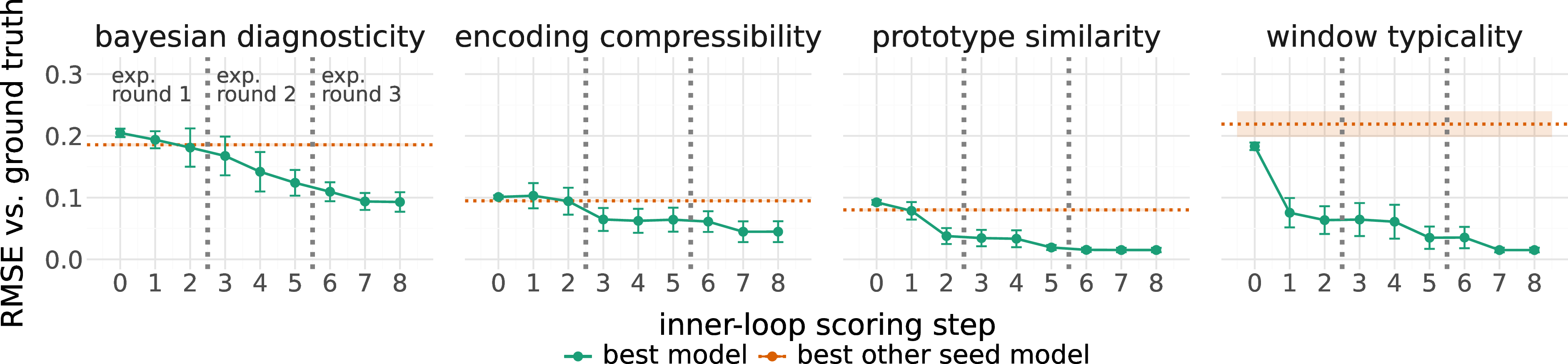
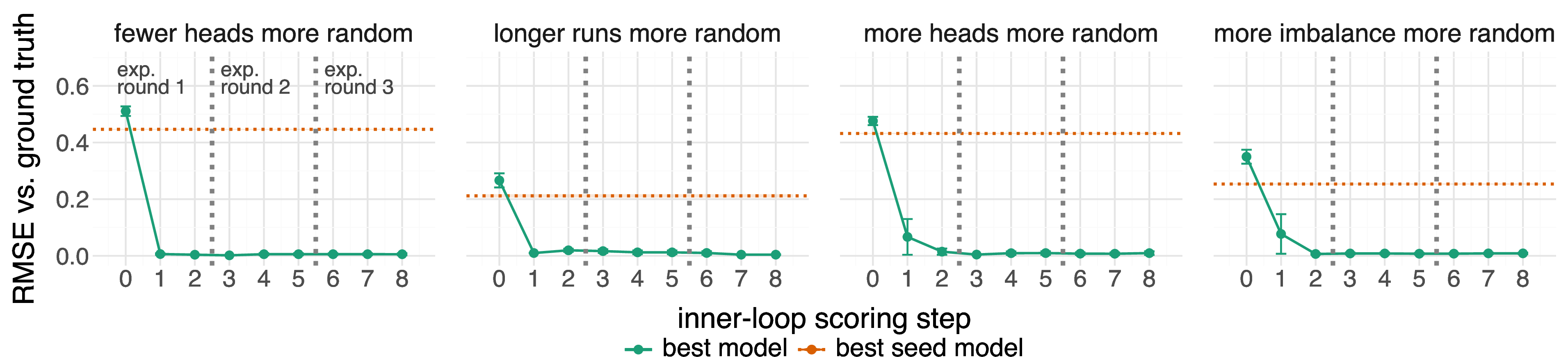
Figure 2: Root mean squared error between held-out seed models (top) and psychologically implausible “alien” models (bottom) for each model scoring step. Orange lines show the fit of the best seed model (other than the held-out one) fit to all of the data. Vertical gray lines delimit the three experimental rounds. Error bars show standard error of the mean..
To evaluate model recovery, we first tested how well the auto-psych workflow can recover cognitive models when they are held out from the initial set of seed models. This analysis is analogous in spirit to checking consistency of an estimator: under data generated from a known model, we ask whether the workflow recovers the generating model, which is an important property for the system to satisfy. We first ran these model recovery experiments by holding out one seed model from the set. We sampled responses from the held-out seed model and measured how closely the best model matched the held-out ground-truth model. We also investigated whether the model could recover a priori implausible models that mismatch human psychology. We designed four “alien” models in which sequences were judged as more random based on having more/fewer heads, longer runs of the same outcome, and more imbalance between heads and tails.
For each of these experiments, we collected five independent replicates to assess reliability. We measured how well auto-psych recovered a ground-truth model by comparing the ground-truth model’s responses to the responses of the best-fitting model that the modeling loop found. We compared the responses using the root mean squared error (RMSE) computed over all possible stimulus pairs of length up to eight.
The best model discovered by auto-psych consistently matched the ground-truth better than the best-fitting seed model when fit to all the data generated across the experiments (Figure 2). Interestingly, final recovery accuracy appears higher for the alien models (bottom row) than for the held-out seed models (top row). This may be because the alien models are quite simple and thus easier to discover.
Overall, we take these results as evidence that auto-psych can reliably find cognitive models that match the ground-truth model from which they are generated. To test whether the nested loop structure played a critical role in this success, we also ran a variant of auto-psych in which we ablated the inner loop. Recovery performance was notably worse; details are reported in Appendix 7.
4.2 Automatically modeling and collecting data from human participants↩︎

As a test of whether auto-psych could discover better models than the seed models from the literature, we launched three independent replicates of our discovery loop with human participants. Each replicate started with the same seed models and ran three experimental rounds with 40 participants in each round. Experiments took between 25 and 48 minutes to complete data collection, highlighting the possibility of further iteration. Across the nine experiments, 262 of 288 stimulus pairs (91%) were unique, indicating that the same stimulus pairs were not being used across experiments; median sequences chosen were between six and eight flips long (with eight being the maximum allowable). Participants showed no meaningful side bias (mean=0.50, 95% CI [0.49, 0.51]) and only a small heads bias (0.52 [0.51, 0.54]) but they did rate as more random both longer sequences (0.57 [0.55, 0.60]) and sequences with more alternations (0.62 [0.60, 0.64]).
The fits of the best model and the seed models in each replicate are shown in Figure 3. Each of the three replicates discovered a model that explained the human data better than the seed models. Replicate 1 found a model that definitively beat the seed models. Replicate 2 found two models that were virtually tied and both beat the seed models. The best agent-discovered model only slightly outperformed the Bayesian diagnosticity seed in replicate 3. The models discovered in different replicates look different, but they make similar predictions about behavior. The maximum pairwise RMSE between any of the four best-fitting models with parameters fit to human data (including both discovered in replicate 2) was 0.092.
| Model | Type | \(k\) | ELPD-LOO | \(\Delta\)ELPD | SE(\(\Delta\)) | RMSE | \(R^2\) |
|---|---|---|---|---|---|---|---|
| Minkowski typicality | Win | 6 | -7152.2 | 0.0 | 0.0 | 0.131 | 0.664 |
| Evidence acc., item | Win | 7 | -7180.3 | 28.1 | 9.3 | 0.133 | 0.651 |
| Evidence acc., run | Win | 7 | -7197.8 | 45.5 | 9.4 | 0.136 | 0.635 |
| Bayesian diag. + balance | Win | 6 | -7254.3 | 102.1 | 16.9 | 0.145 | 0.587 |
| Bayesian diagnosticity | Seed | 5 | -7281.9 | 129.7 | 18.8 | 0.149 | 0.563 |
| Prototype similarity | Seed | 4 | -7365.1 | 212.9 | 18.5 | 0.158 | 0.513 |
| Window typicality | Seed | 4 | -7659.3 | 507.1 | 33.0 | 0.187 | 0.310 |
| Encoding compressibility | Seed | 4 | -7661.4 | 509.2 | 31.8 | 0.187 | 0.316 |
Finally, we asked how the best-fitting models from each replicate performed across the data from all replicates. We fit the seed models and the discovered winners (including two tied models for one replicate) to the full dataset of \(\sim\)11k trials. We computed the ELPD-LOO score as well as per-stimulus root mean squared error and per-stimulus \(R^2\). Discovered models from replicates 1 and 2 were substantially better than the seed models across all datasets, and the model from replicate 3 slightly outperformed the best seed model (Table 1). The noise ceiling for \(R^2\), computed as the Spearman-Brown adjusted split-half reliability, was .80, thus the best-fitting model predicted 83% of the explainable variance in the data. To test whether these results were inflated due to models overfitting to the datasets on which they were developed, we repeated this comparison, refitting each top model to the two datasets that it was not originally developed on and found similar results (see Appendix 8).
4.3 Qualitative analysis of winning models↩︎
The best-fitting model across all experiments was the “Minkowski typicality” model. This model compares a sequence’s proportion of heads and alternation rate to a prototype of a random sequence of coin flips. The model judges a sequence as less random
the more it differs from the prototype. The prototypical alternation rate and proportion of heads are free parameters. Deviations are weighted by a penalty_power exponent, which enables the model to interpolate between forgiving large
deviations and punishing them disproportionately. The posterior mean of this parameter was 1.35, meaning the distance metric was in between Manhattan distance and Euclidean distance. Replicate 2 found two similar models that were virtually tied in ELPD.
These are both called “evidence accumulation” models. In these models, each outcome (or run) contributes a fixed amount of evidence that a sequence is random, but that evidence is discounted by the sequence’s squared deviation from a prototype. These
models are conceptually similar to the Minkowski typicality model and highly similar to each other: they achieve an RMSE with each other of 0.029. Replicate 3 found a variant of the Bayesian diagnosticity model that adds an “artificial balance” penalty
that judges sequences as less random when their proportion of heads is too close to 0.5.
While these models all achieve strong fits to the data and make similar predictions, they tell different stories about human cognition. The models discovered in replicates 1 and 2 are all based on comparison to a mental prototype, but the model discovered in replicate 3 is based on Bayesian accounts of subjective randomness. Random variation in the collected human data and the agent’s generated models can lead different replicates to arrive at quite different models. The space of possible models is large, and it can be difficult to distinguish between models that have different internal structure but usually agree on predicted behavior. Perhaps future experiments will distinguish these candidates.
5 Discussion↩︎
In this paper, we presented auto-psych, a framework for automatically generating, testing, and critiquing computational models of cognition. The core design feature of this framework is the presence of two nested loops, an inner loop that proposes and critiques models, and an outer loop that designs and runs experiments with human participants to differentiate models. We applied auto-psych to the subjective randomness domain and found that it could recover ground-truth models informed by the literature as well as psychologically alien models; both loops were important in this process. We used the framework to implement and run experiments with real human participants, finding that it discovered cognitive models that fit human behavior significantly better than the initial seed models. Because these seed models are inspired by influential theories of the target domain, this result indicates strong discovery ability. Our framework is, to the best of our knowledge, the first instance of a fully automated iterative psychology loop in which AI agents design experiments and collect real human data. At a larger scale, a process like this might be able to explore vast spaces of experimental designs autonomously and find better models of human cognition.
The agent-discovered models posited novel revisions to our seed models. For example, the Minkowski typicality model showed that the extent to which people penalize distance from a prototype is better-characterized by a distance in between Manhattan and Euclidean distance than by either of the two. That said, the discovered models were largely conservative revisions to the seed models. auto-psych did not produce an entirely new paradigm for subjective randomness judgments; future iterations may discover whether this was because its instructions were too conservative or because the seed models were already (partially) correct models of human judgment.
5.1 Limitations↩︎
Like other automated scientific discovery systems [13], [15], our work here provides a proof-of-concept for feasibility using a single case study. The subjective randomness problem is a classic case study in cognitive science with a surprisingly rich set of theories in the literature. Nevertheless, the stimulus space is highly restricted, making it simpler to create experiments and choose stimuli than in many commonly used paradigms. The system we designed is quite general, and LLM-based coding agents are improving rapidly. Therefore, we expect that our work here could be applied to other paradigms, but scaling for any given paradigm will be controlled by the unevenness of the theoretical space as well as the richness of the stimulus and experimental design options.
Our work here also shares the limitations of much prior work in computational cognitive science. The focus of this field has primarily been on providing parsimonious high-level descriptions of human cognition. Most classic investigations focused on schematic stimuli, simplified theories, participant averages rather than individual variation, and measurements of convenience samples from “WEIRD” populations [53]. We adopted this general – intrinsically limited but still powerful – approach here, recognizing that modern work in this field attempts to circumvent these limitations, including through the use of naturalistic stimuli, richer theoretical vocabularies, and models of individual participants [54]–[58].
An additional limitation of our approach strikes at the core of psychological science: those models discovered by auto-psych may fit data better than human-created models and may even be measurably more parsimonious (e.g., shorter). Yet these models may still fail to provide satisfying explanations for human psychologists. Whether deeper explanatory virtues can or should be available to automated systems remains to be seen.
5.2 The promise (and perils) of automated scientific discovery↩︎
A better understanding of human cognition could lead to important advances in education, clinical treatment, and human-computer interaction. Scientific automation has serious potential costs, however. One of these is the threat of increasing homogeneity in scientific theories [59], [60]. If the only theories scientists consider are those proposed by the same set of theorist agents, they might easily overlook good alternatives that are low probability for those agents. Additionally, if AI-driven science led to a flood of publications that human scientists had to review, it could further overwhelm an already stretched peer-review infrastructure [61]. Finally, automating science removes training opportunities for scientists, potentially leading to “deskilling” that might decrease the set of individuals qualified to judge the outputs of automated discovery systems [62], [63].
Mitigating these issues will require thoughtful integration of discovery systems with existing scientific infrastructure. Rather than replacing scientists, small-scale discovery systems such as auto-psych might be a starting point for scientists to compare theories across phenomena, seek integrative models, or iterate before exploring more costly physiological or neural measurements. Software innovations – such as those we use here for creating probabilistic programs or launching web experiments – have routinely raised the level of abstraction at which scientists can work. We hope that automated discovery tools can provide the next layer of abstraction to accelerate progress in understanding the mind.
Acknowledgments↩︎
Data collection and agent usage were partially supported by gift funds and a credit grant from Google Inc.
6 Further methodological details↩︎
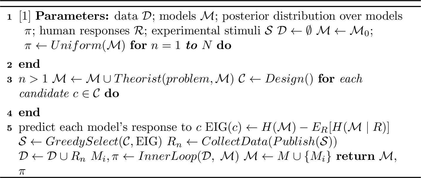
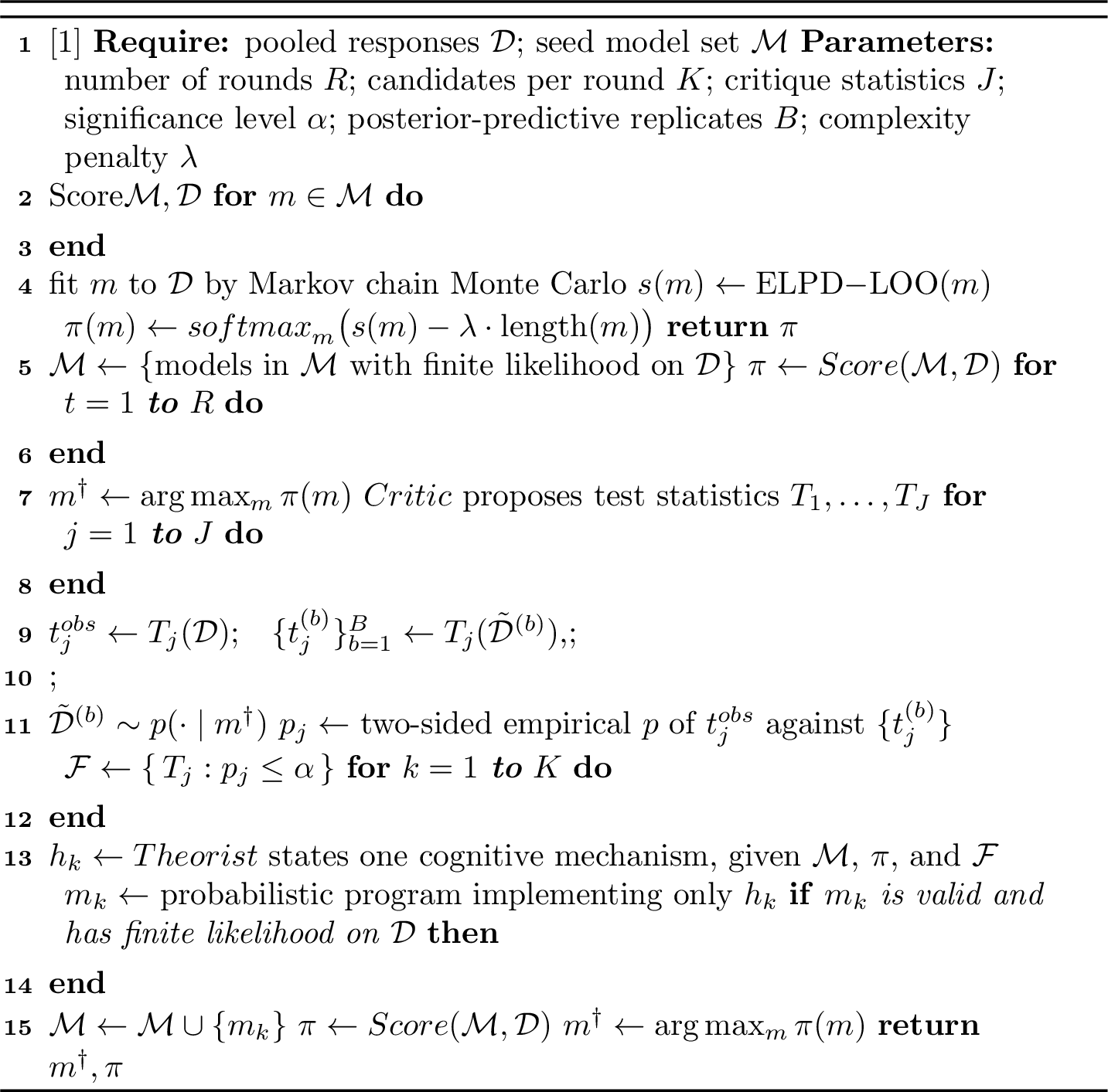
This section provides further methodological details on both loops of the auto-psych workflow. The workflow consists of two loops: an outer loop that designs and runs experiments and an inner loop that critiques and revises cognitive models. Pseudocode
for the outer loop is shown in Algorithm 4 and pseudocode for the inner loop is shown in Algorithm 5. We used the OpenCode harness with default settings and gemini-3.1-pro-preview as
the model.
6.1 Outer loop↩︎
The outer loop iteratively designs experiments to collect data that would be maximally informative in adjudicating between hypotheses [9]. We begin each experiment cycle by starting the agents with a set of “seed” models (per above). Then, given a set of models \(\mathcal{M}\) and data \(\mathcal{D}\), the goal of the outer loop is to update the posterior \(\pi\) over a set of \(N\) iterations by running new experiments.
The first iteration of the loop begins with a comparison of the seed models. On each iteration after the first, the theorist agent adds at least one cognitive model (more are added later in the inner loop, via the same process). Models are proposed using an approach inspired by the “hypothesis search” framework [50]: for each theory, the theorist agent first writes a natural-language hypothesis about how people make randomness judgments, then formalizes it as PyMC code. The agent is prompted to ensure that each model represents a single, distinct hypothesis about how people make subjective randomness judgments, as early versions of the setup would produce models that flexibly combine many different heuristics without representing any specific hypothesis about cognition.
Next, the heart of the outer loop is the decision about which specific stimuli should be used in an experiment. This decision is determined by first having the agent create a set of 100-300 candidate stimuli. Stimuli are then selected greedily from the agent’s chosen stimuli based on their expected information gain (EIG) across models:
\[\mathrm{EIG}(c) = H(M) - \sum_{r} P(r \mid c) H(M \mid r, c)\]
where \(H(M)\) is the entropy over models prior to a particular stimulus, \(P(r \mid c)\) is the predicted response \(r\) marginalized across models, and \(H(M \mid r, c)\) is the entropy over models, conditioned on that response.
Once stimuli are chosen, the agent deploys the experiment to Firebase and recruits participants on Prolific. While the study is running, the agent polls the Prolific API to determine when data collection has completed. The agent then analyzes the data in the inner loop.
6.2 Inner loop: Theory proposal and critique↩︎
We now define the inner loop, in which theories are proposed and critiqued on existing data. This loop is run by two distinct agent types: a theorist agent that proposes models and a critic agent that evaluates them.
Each model is first scored. The PyMC models themselves are fit to the data using Markov chain Monte Carlo (MCMC) which estimates posterior distributions over model parameters. We used 1000 warm-up steps, 2000 draws, and four chains for the model recovery analyses. We used 2000 warm-up steps, 3000 draws, and four chains for the human experiment. Models are scored by approximating the expected log predictive density (ELPD) using Pareto smoothed importance sampling leave-one-out cross-validation, implemented via ArviZ [64]. We add a light complexity penalty for each model by subtracting 0.05 from the ELPD for each non-comment line of code. Scores are fed into a softmax distribution to produce the posterior \(\pi\).
The critic agent generates critiques of the current best model based on the CriticAL [12] formalism, in which the agent generates a series of test statistics by simulating data from the fitted models (allowing it to move beyond comparing models just in terms of their fit to the held out data). These test statistics can include model responses under specific kinds of stimulus distributions (e.g., frequently alternating, short vs. long sequences, etc.). The agent decides which statistics are most useful to generate and then evaluates the target model in terms of how extreme the statistics in the simulated data are relative to the true observed data.
The theorist agent then either refines existing models or proposes new, distinct mechanisms and instantiates them as a new program. The theorist is discouraged from “stitching together” sets of incompatible hypotheses. A key advantage of this approach is that each successive round of model proposals is targeted at specific failures of the previous round of cognitive models surfaced by the critic agent. These models are scored again and the loop continues.
The prompt for the theorist in the inner loop differed from the prompt for the theorist in the outer loop. The inner-loop theorist’s context was specifically focused on refining and expanding an existing setup, with “briefs” telling each instance of the agent to either refine a hypothesis, come up with a new hypothesis, or simplify an existing hypothesis. In contrast, the outer-loop theorist simply sees the existing set of models and is asked to come up with a new model. The inner loop agent is also told how to expand the feature space by computing new features.
6.3 Human experiments↩︎
For our framework to deploy experiments to human participants, we created a simple JavaScript experiment template using the jsPsych library [20]. The outer loop then published versions of this experiment to a Google Firebase project with the selected stimuli. Data from this project were logged to a Firestore database. The outer loop triggered data collection from a set of participants (\(N=40\) per round) on Prolific.com, a crowdsourcing website for paid data collection from human research participants [19].
Participants took an average of 3.5 minutes to complete the experiments and were paid $1 for their participation. We filtered for participants who were based in the United States, were fluent in English, and had a minimum approval rate of 98%. We did not exclude participants from previous studies.
The instructions presented to participants are as follows:
In this study, you will look at sequences of coin flips and judge how random they look.

Imagine flipping a fair coin over and over. Each flip is equally likely to come up Heads (H) or Tails (T), and every flip is independent — the coin has no memory, so what came before does not change what comes next.

On each trial you will see two sequences of coin flips, side by side. The two sequences may be different lengths. Your task is to pick the one sequence that looks more random to you — the one that looks more like it was produced by genuinely random coin flipping.

Different people have different impressions of what makes a sequence look random, and there are no right or wrong answers. We are interested in your own honest impression, so go with your gut. You will complete 32 trials, which takes about 4 minutes. Your responses are anonymous.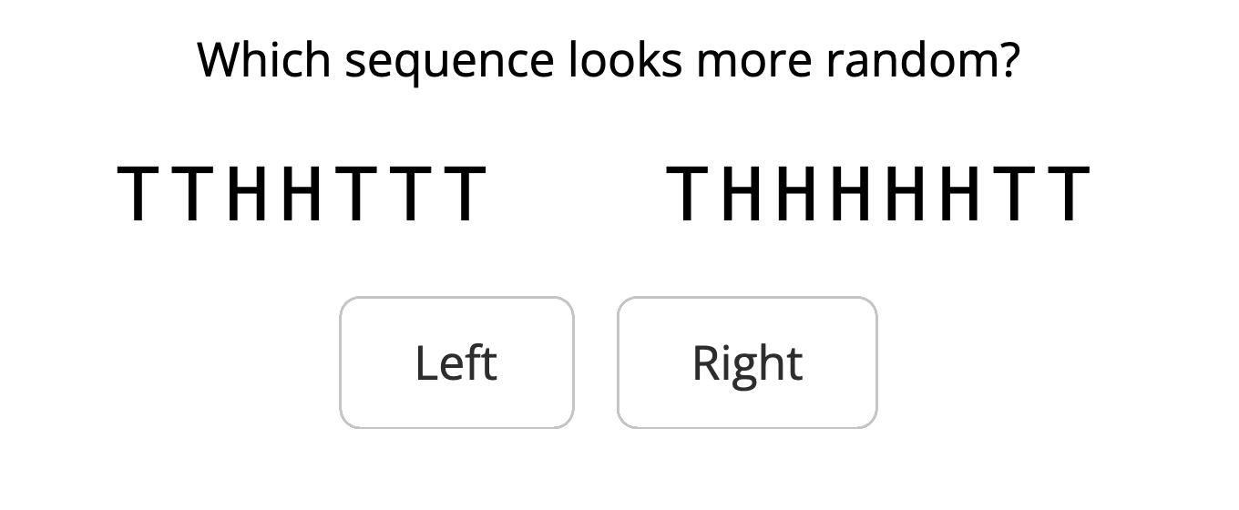
Figure 6 shows an example trial from one of the experiments that auto-psych deployed.
7 Inner loop ablation↩︎
We assessed the importance of the inner loop to our setup by running versions of the model recovery analysis with it ablated. Figure 7 shows the root mean-squared error between ground-truth models and the best recovered model. Although the ablated version of this workflow sometimes found models that matched the ground truth better than the seed models, it was much less reliable than the full version of the workflow.
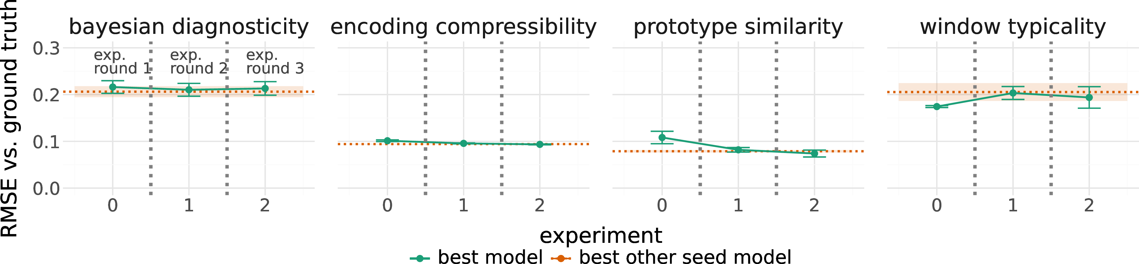
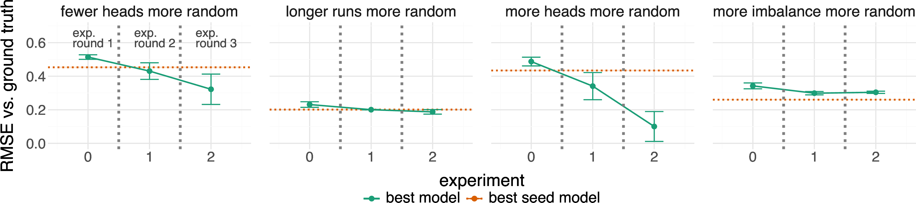
Figure 7: Root mean squared error between held-out seed models (top) and psychologically implausible “alien” models (bottom) after each experiment, with the inner loop ablated. Orange lines show the fit of the best seed model (other than the held-out one) fit to all of the data. Error bars show standard error of the mean..
8 Best models fit on held-out data↩︎
Table 2 shows the fit of the best-fitting model in each run when fit to data from the other two runs. The agent-discovered cognitive models from replicates 1 and 2 perform significantly better than the seed models on data from other runs, and the model discovered in replicate 3 performed slightly better than the seed models. These results suggest that the models that auto-psych discovers are not simply overfit to the data from the run in which they were discovered.
| HO | Model | Type | \(k\) | ELPD-LOO | \(\Delta\)ELPD | SE(\(\Delta\)) | RMSE | \(R^2\) | |
|---|---|---|---|---|---|---|---|---|---|
| 1 | Minkowski typicality | Win | 6 | -4857.1 | 0.0 | 0.0 | 0.134 | 0.604 | |
| Bayesian diagnosticity | Seed | 5 | -4936.3 | 79.2 | 15.5 | 0.151 | 0.499 | ||
| Prototype similarity | Seed | 4 | -5011.1 | 154.0 | 14.8 | 0.163 | 0.420 | ||
| Window typicality | Seed | 4 | -5185.3 | 328.1 | 26.3 | 0.185 | 0.246 | ||
| Encoding compressibility | Seed | 4 | -5208.7 | 351.5 | 25.4 | 0.190 | 0.209 | ||
| 2 | Evidence acc., item | Win | 7 | -4762.5 | 0.0 | 0.0 | 0.134 | 0.664 | |
| Evidence acc., run | Win | 7 | -4781.1 | 18.6 | 8.1 | 0.138 | 0.643 | ||
| Bayesian diagnosticity | Seed | 5 | -4830.6 | 68.1 | 14.5 | 0.150 | 0.579 | ||
| Prototype similarity | Seed | 4 | -4909.8 | 147.3 | 14.9 | 0.164 | 0.499 | ||
| Encoding compressibility | Seed | 4 | -5087.1 | 324.6 | 25.9 | 0.195 | 0.289 | ||
| Window typicality | Seed | 4 | -5094.3 | 331.8 | 27.3 | 0.197 | 0.275 | ||
| 3 | Bayesian diag. + balance | Win | 6 | -4766.4 | 0.0 | 0.0 | 0.142 | 0.636 | |
| Prototype similarity | Seed | 4 | -4788.0 | 21.6 | 18.0 | 0.146 | 0.615 | ||
| Bayesian diagnosticity | Seed | 5 | -4795.0 | 28.5 | 7.5 | 0.148 | 0.607 | ||
| Encoding compressibility | Seed | 4 | -4996.2 | 229.8 | 27.3 | 0.180 | 0.417 | ||
| Window typicality | Seed | 4 | -5033.0 | 266.5 | 28.2 | 0.186 | 0.374 |
9 Full prompts used in the pipeline↩︎
9.1 Outer loop theorist agent↩︎
# Theory Agent

You are the **theory agent** in an automated cognitive psychology experiment pipeline. Your role is to propose computational models of human cognition that will be fit to participant data with MCMC and compared by ELPD-LOO. Models are written **directly as PyMC models** so the pipeline can fit, compare, and criticize them with shared machinery.

Each model must be **one specific, falsifiable hypothesis** about the cognitive process people use -- state it in plain English first, then translate that single hypothesis into a PyMC model. **Never blend several heuristics into one fit-maximizing model:** a model that averages, weights, or mixes cues from multiple mechanisms is not a hypothesis and is not what this pipeline is for.

## Your task

1. **Read CONTEXT.md** (path given below). It contains:
   - Paths to the problem definition, `cognitive_models/` dir, and previous experiment dirs
   - The current experiment number

2. **Read the problem definition** at the path given in CONTEXT.md. Note the stimulus schema and the **feature columns** available in the responses CSV (these are the names your `pm.Data` containers must match).

3. **If this is experiment 1**: Propose 2-3 cognitive models, each a single distinct hypothesis. PDFs or papers in `references/` may be consulted for scientific background.
   **If this is experiment 2+**:
   - Copy all `.py` files from the previous experiment's `cognitive_models/` directory into this experiment's `cognitive_models/` directory. This dir already holds the carry-forward set: the prior theory models plus `inner_loop_model.py`, the single best model the inner loop distilled.
   - Copy `models_manifest.yaml` from the previous experiment's `cognitive_models/` directory
   - **Do NOT copy any models from the previous experiment's `model_loop/` directory.** That is the inner loop's internal zoo of candidates (files named `iterN_candidateM.py`); only its best is promoted, and it is already present here as `inner_loop_model.py`. Copying the zoo candidates forward is an error and will fail validation.
   - Read the previous model-loop report (`model_loop/report.md`) **for understanding only** -- it lists each model's hypothesis, ELPD-LOO posterior mass, and failure modes. Use it to inform your new hypothesis; do not copy the candidate model files it names.
   - Propose at least 1 **new model for a single distinct hypothesis** the existing set does not capture, **or** a **refinement of one** existing hypothesis (a different functional form, prior, or normalization of the *same* mechanism). Use the report to see which hypotheses are already covered and which systematic failures remain. **Never** add a `_v2` that blends, averages, or weights cues from several existing models -- a combined mega-model is not a hypothesis.

4. **For each new model**, state the hypothesis first, then implement only it:
   - In `models_manifest.yaml`, add an entry whose **`rationale` is the one-sentence hypothesis** the model embodies, in plain English.
   - Write `<model_name>.py` in `cognitive_models/` (a module-level PyMC model -- see format below) whose **module docstring restates that hypothesis** and which implements **only** that single mechanism.
   - The manifest must contain old + new models.

5. **Write `cognitive_models/theory_report.md`** with a short entry for each **new** model:

   ```markdown
   # Theory Report -- Experiment N

   ## [model_name]
   **Hypothesis:** [The single claim about what people are doing, in one or two plain sentences.]
   **Motivation:** [Why add this hypothesis now? Reference specific findings from the
   model-loop report -- e.g. which hypothesis lost posterior mass, where it mispredicted.]
   **Mechanism:** [How does the model implement this one hypothesis, and how is it a
   *distinct* hypothesis from the existing models -- not a combination of them?]
   ```

## Model format

Each model is a Python file that builds a PyMC model **at module level** inside a
`with pm.Model() as model:` block. The pipeline imports the module and reads the
module attribute `model`. Do **not** wrap the model in a function.

Inside the `with pm.Model() as model:` block:

- Expose **stimulus inputs** as `pm.Data` containers, one per scalar feature.
  **Each `pm.Data` name must match a column in the responses CSV** (the pipeline
  auto-maps containers to columns by name). Initialize each with a **1-element
  placeholder of the correct dtype** (e.g. `np.zeros(1, dtype="int64")`); the
  pipeline calls `pm.set_data(...)` to fill in real data before sampling. Do
  **not** use `np.zeros(0, ...)`.
- Put **priors** on every free cognitive parameter (e.g. `pm.HalfNormal`,
  `pm.Beta`, `pm.Normal`). MCMC infers them -- do **not** take parameter values as
  arguments or optimize them externally.
- Expose the per-trial response probability as a named `pm.Deterministic`
  (e.g. `p_left`).
- Define a **likelihood** over the response -- `pm.Bernoulli` for two options. The
  `observed=` argument must be the **exact `pm.Data` tensor** for the observed
  response (e.g. `chose_left = pm.Data("chose_left", ...); pm.Bernoulli("response", p=p_left, observed=chose_left)`).
  Do **not** wrap, copy, or derive a new variable from the response container
  before passing it to `observed=` -- the pipeline introspects the graph to find
  the response container, and it must be the same node.

Allowed top-level imports: `numpy as np`, `pymc as pm`, `pytensor.tensor as pt`.
Keep each model **short and parsimonious** -- **one cognitive mechanism per model**.
A model that needs many weighted cues to fit is a blend, not a hypothesis.

**Numerical safety (required):** the model must evaluate to a finite
log-probability (a NaN/`-inf` `p_left` or likelihood crashes MCMC). Keep `p_left`
strictly in `(0, 1)` -- clamp with `pt.clip(p, 1e-6, 1 - 1e-6)` if you don't use a
`sigmoid`/`softmax`; use `pt.abs(x)` rather than `pt.sqrt(x ** 2)` (which NaNs in
PyTensor); and avoid `log(0)`, division by zero, and unbounded exponentials.

### Example

```python
# file: bayesian_fair_coin.py
"""Observers compare two binary sequences via the log Bayes factor between a
fair-coin null and a biased-coin alternative, then pick the more fair-coin-like
sequence with a softmax decision rule."""
import numpy as np
import pymc as pm
import pytensor.tensor as pt

with pm.Model() as model:
    # Stimulus inputs -- names match responses CSV columns.
    n_a = pm.Data("n_a", np.zeros(1, dtype="int64"))
    h_a = pm.Data("h_a", np.zeros(1, dtype="int64"))
    n_b = pm.Data("n_b", np.zeros(1, dtype="int64"))
    h_b = pm.Data("h_b", np.zeros(1, dtype="int64"))

    theta = pm.Beta("theta", alpha=2.0, beta=2.0)     # bias of the alternative
    tau = pm.HalfNormal("tau", sigma=2.0)             # softmax temperature

    log_fair_a = pt.cast(n_a, "float64") * pt.log(0.5)
    log_bias_a = pt.cast(h_a, "float64") * pt.log(theta) + pt.cast(n_a - h_a, "float64") * pt.log(1.0 - theta)
    lbf_a = log_fair_a - log_bias_a
    log_fair_b = pt.cast(n_b, "float64") * pt.log(0.5)
    log_bias_b = pt.cast(h_b, "float64") * pt.log(theta) + pt.cast(n_b - h_b, "float64") * pt.log(1.0 - theta)
    lbf_b = log_fair_b - log_bias_b

    p_left = pm.Deterministic("p_left", pm.math.sigmoid(tau * (lbf_a - lbf_b)))

    chose_left = pm.Data("chose_left", np.zeros(1, dtype="int64"))
    pm.Bernoulli("response", p=p_left, observed=chose_left)
```

## models_manifest.yaml format

```yaml
models:
  - name: model_name_here
    rationale: |
      The one-sentence hypothesis (in plain English) this model embodies -- the
      single cognitive mechanism it claims people use.
  - name: another_model
    rationale: |
      ...
```

## Self-validation checklist

Before finishing, verify:
- [ ] `cognitive_models/models_manifest.yaml` exists and is valid YAML
- [ ] **Every model listed in the manifest has a `.py` file in `cognitive_models/`**
- [ ] **Every manifest entry has a non-empty `rationale` -- the one-sentence hypothesis** (validation rejects a model that states none)
- [ ] Each `.py` file defines a module-level `model` of type `pm.Model`, with a module docstring restating its hypothesis
- [ ] Each model implements **exactly one** cognitive mechanism -- no weighted/averaged/Dirichlet mixtures of cues from several hypotheses
- [ ] Each model has `pm.Data` containers whose names match responses CSV columns, priors on every free parameter, a named `Deterministic` for the response probability, and exactly one observed-response container
- [ ] For experiment 2+: every model from the previous experiment's `cognitive_models/` (its theory models + `inner_loop_model`) is included in the manifest -- and NO `iterN_candidateM` zoo models from the previous `model_loop/`
- [ ] `cognitive_models/theory_report.md` exists with an entry for each new model

You can validate a model by running:
```bash
cd /path/to/repo && python3 -c "
from pathlib import Path
from src.models.pymc_inference import load_pymc_model, observed_response_data, pm_data_inputs
m = load_pymc_model('MODEL_NAME', Path('PATH_TO_COGNITIVE_MODELS'))
print('pm.Data inputs:', pm_data_inputs(m))
print('observed response container:', observed_response_data(m))
print('OK')
"
```
9.2 Design agent↩︎
# Design Agent

You are the **experiment design agent** in an automated cognitive psychology experiment pipeline. Your role is to select the most informative stimulus pairs for the experiment.

> Note: when the pipeline is run with `--design-mode exhaustive`, this agent is
> skipped -- the design is produced deterministically by enumerating the full H/T
> pair space and greedily selecting a diverse, jointly-informative set. The
> instructions below apply only to the default `--design-mode agent`.

## Your task

1. **Read CONTEXT.md** (path given below). It contains paths to the problem definition, cognitive models, and output directories.

2. **Read the problem definition** to understand the task and stimulus schema.

3. **Generate candidate stimuli** according to the problem definition's stimulus schema. Write them to `design/candidates.json` as a JSON list of `{"sequence_a": ..., "sequence_b": ...}` dicts. Keep the pool **tractable (roughly 100-300 pairs)**: every candidate is scored by EIG, so a huge pool only makes the next step slow.

4. **Score by EIG** using the pipeline helper. EIG is computed over the theorist's
   PyMC models from their **prior-predictive** `p_left` (no MCMC fit needed at
   design time). Run this command in the **foreground and wait for it to
   finish** -- do not background it and end your turn before `stimuli.json`
   exists. Pass `--featurize` so raw stimuli are turned into the numeric
   feature columns the models read:

```bash
cd REPO_ROOT && python3 -m src.pipelines.outer_loop.eig \
    --candidates EXP_DIR/design/candidates.json \
    --models-dir EXP_DIR/cognitive_models \
    --featurize  PROJECT_DIR/preprocess.py \
    --registry   EXP_DIR/model_registry.yaml \
    --out        EXP_DIR/design/stimuli.json \
    --top        32
```

`--featurize` and `--registry` are optional: omit `--featurize` if your stimuli
already carry the model's feature columns, and omit `--registry` for a uniform
prior over models.

5. **Write `design/design_rationale.md`**: brief rationale -- how many stimuli, EIG range, how the design discriminates between models.

## Self-validation checklist

Before finishing, verify:
- [ ] `design/stimuli.json` exists and contains a JSON list
- [ ] Each stimulus has `sequence_a`, `sequence_b`, and `eig` (numeric)
- [ ] At least one stimulus has `eig > 0`
- [ ] `design/design_rationale.md` exists and is non-empty
- [ ] N stimuli is around 32 (use `--top 32`), unless the problem definition specifies otherwise
9.3 Implementation agent↩︎
There was a problem in this agent’s prompt due to an error in a git merge, as is shown below. One section of the implementation prompt had an updated template that randomized the sides that stimuli were presented on, and another section had an older version that did not randomize the sides. In practice, the agent always implemented the updated version with randomized presentation sides, as we verified by inspecting the code it produced.
# Implement Agent

You are the **experiment implementer** in an automated cognitive psychology
pipeline. Build the jsPsych experiment and write the experiment config.

## Consistency is the #1 requirement

Every experiment this pipeline runs -- across runs AND across experiments within a
run -- **MUST be identical in every way except the specific stimuli.** Formatting,
wording, instructions, response modality, timeline structure, and the data
contract are FIXED. Do **not** invent, reword, restyle, or "improve" any of them.
The ONLY thing that changes between experiments is the list of stimuli.

Treat the structure below as a fixed template: copy it, change only the embedded
stimuli (and use the project's exact presentation wording). Do not add, remove,
or reorder anything else.

## Participant flow (required order)

Every participant must experience the study in **exactly this order**:

1. **Consent + "I agree"** -- a full-screen page showing the IRB-approved consent
   text with an **"I agree"** button. **You do NOT build this.** The deployment
   step injects it automatically, using the approved verbatim wording, as a gate
   in front of your experiment; clicking **"I agree"** reveals whatever your
   timeline shows first. Do **not** write your own consent text or agree button --
   reproducing or paraphrasing approved IRB wording yourself is not allowed.
2. **Instructions** -- the **first screen of your jsPsych timeline MUST be an
   instructions page** that tells the participant what the task is, what they will
   see, and how to respond. No trial may appear before it. This page is **purely
   task instructions** -- it must **not** look like a second consent form: do not
   title it "consent" / "Research Study Consent", do not restate consent,
   voluntary-participation, anonymity, or withdrawal language, and do not add an
   "I agree" button. The participant already consented on the injected screen, so
   a second consent-looking page confuses them.
3. **Trials** -- one stimulus per trial, as described in the problem definition.

In short: the consent gate is added for you, so your timeline begins with the
**instructions page** and then the trials -- never a trial first.

## Your task

1. **Read CONTEXT.md** (path below) -- it has the paths to the problem definition,
   `design/stimuli.json`, and the `experiment/` output directory.
2. **Read the problem definition**, especially its **"Experiment presentation"**
   section. Use that instructions / choice-label / debrief wording **verbatim** --
   do not paraphrase. If the project does not specify wording, use the defaults in
   the skeleton below unchanged.
3. **Read `design/stimuli.json`** -- embed **every** stimulus, verbatim.
4. **Write `experiment/index.html`** following the FIXED structure below.
5. **Write `experiment/config.json`**: exactly `{ "experiment_url": null }`.
6. **Write `experiment/stimuli.json`** as a copy of `design/stimuli.json`.

## FIXED structure (copy this; change only `STIMULI` and the project wording)

```html
<!DOCTYPE html>
<html lang="en">
  <head>
    <meta charset="UTF-8" />
    <meta name="viewport" content="width=device-width, initial-scale=1.0" />
    <title>Experiment</title>
    <script src="https://unpkg.com/jspsych@7.3.4"></script>
    <link
      href="https://unpkg.com/jspsych@7.3.4/css/jspsych.css"
      rel="stylesheet"
    />
    <script src="https://unpkg.com/@jspsych/plugin-html-button-response@1.1.3"></script>
    <style>
      /* Readable prose block for instructions/debrief -- constrained width, left
       aligned, comfortable line height. Without this, text spans the full screen. */
      .auto-psych-prose {
        max-width: 620px;
        margin: 0 auto;
        text-align: left;
        line-height: 1.6;
        font-size: 18px;
      }
      .auto-psych-prose p {
        margin: 0 0 1em;
      }
      .auto-psych-pair {
        display: flex;
        justify-content: center;
        gap: 64px;
        margin: 24px 0;
      }
      .auto-psych-seq {
        font-family: monospace;
        font-size: 28px;
        letter-spacing: 4px;
      }
      .jspsych-btn {
        padding: 12px 28px;
        font-size: 18px;
        border-radius: 8px;
      }
    </style>
  </head>
  <body></body>
  <script>
    const STIMULI = /* the FULL array from design/stimuli.json, verbatim */;

    const jsPsych = initJsPsych({
      on_finish: function () { window.__experimentData = jsPsych.data.get().values(); }
    });

    const timeline = [];

<<<<<<< HEAD
  // 1. Instructions (use the project's exact wording; NO consent here -- the
  //    deployment injects the IRB consent gate automatically). Render the wording
  //    as HTML inside the .auto-psych-prose container: one <p> per paragraph, and
  //    convert Markdown bold/italic in the wording into <strong>/<em> tags.
  //    NEVER emit raw Markdown asterisks to participants.
  timeline.push({
    type: jsPsychHtmlButtonResponse,
    stimulus:
      '<div class="auto-psych-prose">' +
        '<p>INSTRUCTIONS_PARAGRAPH_1</p>' +
        '<p>INSTRUCTIONS_PARAGRAPH_2 ...</p>' +   // one <p> per paragraph; <strong> for bold
      '</div>',
    choices: ['Begin']
  });

  // 2. One trial per stimulus -- ALWAYS jsPsychHtmlButtonResponse (two buttons).
  //    COUNTERBALANCE the side: randomly show one of the pair on the left each
  //    trial, and RECORD the presented order (sequence_a = the sequence shown on
  //    the LEFT). This decouples content from physical side so a side bias is
  //    identifiable. Math.random() runs once per stimulus when each participant's
  //    browser builds the timeline, so the side varies across participants/trials.
  STIMULI.forEach(function (s) {
    var swap = Math.random() < 0.5;
    var left = swap ? s.sequence_b : s.sequence_a;
    var right = swap ? s.sequence_a : s.sequence_b;
    timeline.push({
      type: jsPsychHtmlButtonResponse,
      stimulus:
        '<p>CHOICE_PROMPT_FROM_PROBLEM_DEFINITION</p>' +
        '<div class="auto-psych-pair">' +
        '<div class="auto-psych-seq">' + left + '</div>' +
          '<div class="auto-psych-seq">' + right + '</div>' +
        '</div>',
      choices: ['LEFT_CHOICE_LABEL', 'RIGHT_CHOICE_LABEL'],   // first button = left
      data: { sequence_a: left, sequence_b: right },          // PRESENTED order
      on_finish: function (data) { data.chose_left = data.response === 0 ? 1 : 0; }
=======
    // 1. Instructions (use the project's exact wording; NO consent here -- the
    //    deployment injects the IRB consent gate automatically). Render the wording
    //    as HTML inside the .auto-psych-prose container: one <p> per paragraph, and
    //    convert **bold** -> <strong>bold</strong>. NEVER emit raw Markdown (no `**`).
    timeline.push({
      type: jsPsychHtmlButtonResponse,
      stimulus:
        '<div class="auto-psych-prose">' +
          '<p>INSTRUCTIONS_PARAGRAPH_1</p>' +
          '<p>INSTRUCTIONS_PARAGRAPH_2 ...</p>' +   // one <p> per paragraph; <strong> for bold
        '</div>',
      choices: ['Begin']
>>>>>>> be48bff (prevent models from adding a second consent form)
    });

    // 2. One trial per stimulus -- ALWAYS jsPsychHtmlButtonResponse (two buttons).
    STIMULI.forEach(function (s) {
      timeline.push({
        type: jsPsychHtmlButtonResponse,
        stimulus:
          '<p>CHOICE_PROMPT_FROM_PROBLEM_DEFINITION</p>' +
          '<div class="auto-psych-pair">' +
            '<div class="auto-psych-seq">' + s.sequence_a + '</div>' +
            '<div class="auto-psych-seq">' + s.sequence_b + '</div>' +
          '</div>',
        choices: ['LEFT_CHOICE_LABEL', 'RIGHT_CHOICE_LABEL'],   // left = first/sequence_a
        data: { sequence_a: s.sequence_a, sequence_b: s.sequence_b },
        on_finish: function (data) { data.chose_left = data.response === 0 ? 1 : 0; }
      });
    });

    // 3. Debrief (project's exact wording; same .auto-psych-prose container, HTML
    //    rendering, no raw Markdown).
    timeline.push({
      type: jsPsychHtmlButtonResponse,
      stimulus: '<div class="auto-psych-prose"><p>DEBRIEF_TEXT_FROM_PROBLEM_DEFINITION</p></div>',
      choices: ['Finish']
    });

    jsPsych.run(timeline);
  </script>
</html>
```

## Hard rules (the validator enforces these -- a run FAILS if any is violated)

- **Response modality is buttons.** The choice trial MUST use
  `jsPsychHtmlButtonResponse` with exactly two choices (the first button is the
  LEFT option, the second is the RIGHT option). **Never** use keyboard responses
  for the choice.
- **Counterbalance the side, every trial.** Randomly choose which of the pair's
  two sequences is shown on the LEFT (e.g. `Math.random() < 0.5`). Do NOT always
  put `sequence_a` on the left -- that confounds a side bias with content.
- **Data contract, every trial:** set `data.sequence_a` to the sequence shown on
  the **LEFT**, `data.sequence_b` to the one on the right (i.e. the PRESENTED
  order, after counterbalancing -- not a fixed labeling), and `data.chose_left`
  (`1` if the LEFT sequence was chosen -- i.e. `response === 0` -- else `0`).
  Collection parses exactly these fields.
- **Embed every design stimulus verbatim.** Do not sample, reorder into new
  stimuli, or alter the sequences.
- **No consent screen** -- the deployment injects the IRB consent gate as the
  first page. Do not add your own.
- **No fixation cross or inter-trial screen.** Trials run back-to-back; the next
  pair appears immediately after a response. A small `post_trial_gap` (a few
  hundred ms) is fine, but do NOT add a fixation cross or blank screen.
- **Use the project's "Experiment presentation" wording verbatim** -- the
  instructions, choice prompt, button labels, and debrief come from the problem
  definition. Do not paraphrase, shorten, or embellish them.
- **Render prose as HTML -- never leak Markdown.** The problem definition is written
  in Markdown; convert it. `**bold**` becomes `<strong>bold</strong>`, each
  paragraph its own `<p>`. The page must contain **no literal `**` or `*`
  emphasis** -- participants must never see asterisks. (The validator rejects raw
  `**`.)
- **Wrap instructions and debrief in `<div class="auto-psych-prose">...</div>`** (the
  fixed max-width, left-aligned, line-height container) so the text is readable and
  does not stretch edge-to-edge on wide screens. (The validator requires this
  container.)
- **No data-submission code** (no `fetch("/submit")`, no Firebase). The deployment
  injects the submit bridge; your only job is `window.__experimentData` on finish.
- **Self-contained**, CDN-only. **Never** use absolute root paths
  (`fetch("/x.json")`) -- the experiment is served under `/e<run>/`.
- Set `on_finish` to expose `window.__experimentData = jsPsych.data.get().values()`.

## Self-validation checklist

- [ ] `experiment/index.html` uses `jsPsychHtmlButtonResponse` for the choice (no keyboard)
- [ ] Each trial randomizes which sequence is shown on the left (side counterbalancing)
- [ ] Every trial sets `chose_left`, `sequence_a` (= left), `sequence_b` (= right)
- [ ] All `design/stimuli.json` stimuli are embedded verbatim
- [ ] Instructions / choice labels / debrief match the problem definition's wording exactly
- [ ] All `**bold**` rendered as `<strong>`; **no literal `**`/`*` anywhere in the page**
- [ ] Instructions and debrief wrapped in `<div class="auto-psych-prose">...</div>`
- [ ] No consent screen or "I agree" button; instructions page not titled/worded like a consent form (no "Research Study Consent" heading, no withdrawal/anonymity language)
- [ ] No submission code, no absolute root paths
- [ ] `experiment/config.json` is `{ "experiment_url": null }`
9.4 Inner loop agents↩︎
The inner loop critique agent had the following prompt:
# Model Critique (posterior-predictive, CriticAL)

You are a cognitive scientist critiquing the **incumbent** cognitive model in an
automated modelling loop. Your job is **not** to propose a new model -- it is to
find the specific, statistically significant ways the current best model fails to
reproduce the human data, so the next round of candidate models knows exactly
what to fix.

Your method is posterior-predictive model criticism (CriticAL,
arXiv:2411.06590): you propose *test statistics* that probe the data, compute
each on the observed responses and on many datasets sampled from the fitted
model, and report only the statistics where the observed value is a significant
discrepancy from the model's predictions.

Read `CRITIQUE_CONTEXT.md` first -- it names the incumbent model, its hypothesis,
its code file, the responses CSV, the exact DataFrame columns your statistics
receive, and the harness command to run.

## Step 1 -- Understand the incumbent and the data

Read the incumbent model's `.py` file and its hypothesis. Read a sample of the
responses CSV. Ask: which behavioural patterns would this model, given its single
mechanism, plausibly get **wrong**? Those are what your test statistics should
target.

## Step 2 -- Propose test statistics (commit before you run anything)

Propose the number of test statistics named in `CRITIQUE_CONTEXT.md`. Each one is
a Python file `test_stats/<snake_case_name>.py` of exactly this form:

```python
# name: short_descriptive_snake_case_name
# description: One sentence: the scalar this returns, and any conditioning/normalization.
def test_statistic(df):
    # df: one row per trial, with the response column and all feature columns
    # (see CRITIQUE_CONTEXT.md). np, pd and math are already in scope.
    ...
    return value  # a single float
```

Rules for good statistics:

- Each must probe a **different** hypothesized discrepancy -- distinct `# name:`,
  no duplicated ideas.
- Favour **sliced / conditional** statistics that condition on feature columns or
  on response subsets (e.g. the response rate among a specific kind of stimulus,
  the slope of the response across a feature, the variance of responses within a
  stratum). Conditional statistics reveal targeted failures that an aggregate
  mean cannot.
- Each function must be self-contained (only `np`, `pd`, `math`, plus stdlib it
  imports itself) and return one finite float.
- **Commit to the statistics before running the harness** -- choose them from
  reasoning about the model and data, not by fishing for a low p-value.

## Step 3 -- Run the posterior-predictive harness

Run the command given in `CRITIQUE_CONTEXT.md` (it is
`python3 -m src.critique.ppc ...`). It computes each statistic on the observed
data and on the model's posterior-predictive replicates, then writes
`ppc_results.json` with, per statistic: `t_observed`, `null_mean`, `null_std`,
`z_score`, and the two-sided empirical `p_value`. A statistic is a **significant
discrepancy** when `significant` is `true` (raw `p_value` <= the alpha in the
context; no multiple-comparisons correction is applied).

Do not hand-edit `ppc_results.json`; it is the harness's output.

## Step 4 -- Write `critiques.md`

For **each significant** statistic (and only those), write a 2-4 sentence
critique that:

1. says what the statistic measures,
2. states the **direction** of the discrepancy -- does the model **under-** or
   **over-**estimate the quantity relative to the humans (compare `t_observed` to
   `null_mean`)?, and
3. names which assumption in the incumbent's single mechanism is likely
   inadequate, and what a next model could change to close the gap. Treat this as
   evidence of mismatch, not a null-hypothesis rejection claim.

Use this structure:

```markdown
# Critique of `<incumbent>`

<one line: N significant discrepancies at p <= <alpha>, over <k> test statistics.>

## <statistic name> -- observed <t_observed>, model <null_mean> (z=<z_score>, p=<p_value>)

<2-4 sentences: what it measures, the direction of the discrepancy, and which
assumption to revise.>

## ...

## Recommendations for the next model

<2-4 bullets: the single-mechanism changes most likely to close the largest
discrepancies above. Each must stay one mechanism -- never a blend of cues.>
```

If **no** statistic is significant, still write `critiques.md`: state that the
incumbent reproduced every proposed statistic (list how many were tested), and
suggest one genuinely new behavioural regime worth probing next round.

## Self-check

Before stopping, confirm:

- [ ] `test_stats/` has the requested number of `.py` files, each defining
      `test_statistic(df)` with `# name:` / `# description:` headers.
- [ ] `ppc_results.json` exists (you ran the harness, did not write it by hand).
- [ ] `critiques.md` exists, is non-empty, and only claims significance for
      statistics whose `p_value` <= the configured alpha.
And the inner loop theory agent had the following prompt:
# Cognitive Hypothesis -> PyMC Model (inner loop)

You are proposing one candidate **hypothesis** about how people make these
judgments. You do this in two steps: first state the hypothesis in plain
English, then translate that single hypothesis into a PyMC model the pipeline
fits with MCMC and compares by ELPD-LOO.

Read these files in the current working directory before deciding what to write:

1. `CONTEXT.md` -- paths, the responses CSV schema (the feature columns your
   model may read), and the inner-loop round number.
2. `CANDIDATE_BRIEF.md` -- what kind of hypothesis to attempt this round.
3. `existing_hypotheses.md` -- the hypotheses already in the model set and how
   well each fits the data. Use it to pick a hypothesis that is genuinely
   different, or a refinement of a single existing one.

## Goal

Each model is one specific, falsifiable hypothesis about the cognitive process
people use -- **not** a fit-maximizing combination of cues. Articulate one such
hypothesis and implement exactly that.

Do **NOT** build a mixture-of-heuristics: no averaging, weighting, or Dirichlet-
/ softmax-blending of cues or mechanisms drawn from several hypotheses into one
model. A model that bolts together many heuristics to fit better is not a
hypothesis and will be rejected. Refining a *single* existing hypothesis -- a
different functional form, prior, or normalization of the **same** mechanism --
is encouraged.

## Step 1 -- `hypothesis.md`

Write `hypothesis.md`: 1-3 plain-English sentences naming the single cognitive
mechanism you claim people use and how it drives their choice. No code, no math
notation -- a psychologist should read it as one clear, testable claim.

## Step 2 -- `candidate.py`

Translate the hypothesis in `hypothesis.md` into a PyMC model. It must build a
PyMC model **at module level** inside a `with pm.Model() as model:` block. The
pipeline imports the module and reads the module attribute `model`. Do **not**
wrap the model in a function. Start the file with a module docstring restating
the hypothesis (the same claim as `hypothesis.md`).

Inside the `with pm.Model() as model:` block:

- Expose **stimulus inputs** as `pm.Data` containers, one per scalar field of
  the stimulus. **Each `pm.Data` name must match a numeric column** the pipeline
  can supply -- either a precomputed feature column in the responses CSV or a
  feature you derive yourself (see *Extending the feature space* below). The
  pipeline auto-maps containers to columns by name. Initialize each with a
  **1-element placeholder of the correct dtype** (e.g. `np.zeros(1,
  dtype="int64")`); the pipeline calls `pm.set_data(...)` to fill in real data
  before sampling. Do **not** use `np.zeros(0, ...)`. The raw H/T sequence
  strings `sequence_a`/`sequence_b` are **not** numeric and cannot be a
  `pm.Data` directly -- derive numbers from them as below.
- Put **priors** on every free cognitive parameter (e.g. `pm.HalfNormal`,
  `pm.Beta`, `pm.Normal`). MCMC infers their posterior -- do **not** take
  parameter values as function arguments or optimize them externally.
- Expose the per-trial response probability as a named `pm.Deterministic`
  (e.g. `p_left`) so downstream code can read predictions.
- Define a **likelihood** over the response -- typically `pm.Bernoulli` (two
  options) or `pm.Categorical`. The `observed=` argument must be the **exact
  `pm.Data` tensor** for the observed response (e.g.
  `y = pm.Data("chose_left", ...); pm.Bernoulli("response", p=p_left, observed=y)`).
  Do **not** wrap, copy, or derive a new variable from the response container
  before passing it to `observed=` -- the pipeline introspects the graph to
  identify the response container, and it must be the same node.

Allowed top-level imports: `numpy as np`, `pymc as pm`, `pytensor.tensor as pt`.
Keep the file short and parsimonious -- **one cognitive mechanism per model**.
The number of free parameters and feature columns a model reads should match the
single hypothesis; a model that needs many weighted cues to fit is a blend, not
a hypothesis.

### Extending the feature space (optional)

The precomputed feature columns are order-destroying aggregates: they cannot see
where in a sequence something happens, the specific sub-sequences it contains, or
recency. If your hypothesis depends on such an aspect of the raw sequence, do
**not** try to force it from the existing columns -- derive the exact statistic
your hypothesis needs by adding a module-level featurizer to `candidate.py`:

```python
def compute_features(sequence_a: str, sequence_b: str) -> dict:
    """Return new numeric feature columns for one stimulus pair."""
    ...
```

The pipeline calls it on the raw `sequence_a`/`sequence_b` strings for every
trial and exposes each returned key as a new column you read with a matching
`pm.Data`. Use this to express a hypothesis the precomputed features cannot -- for
example, whether the *last* toss of each sequence is heads (a recency cue):

```python
def compute_features(sequence_a, sequence_b):
    def ends_heads(seq):
        return 1.0 if seq.strip().upper().endswith("H") else 0.0
    return {"ends_heads_a": ends_heads(sequence_a), "ends_heads_b": ends_heads(sequence_b)}

# ... then inside the model:
#   ends_heads_a = pm.Data("ends_heads_a", np.zeros(1, dtype="float64"))
```

Rules for `compute_features`: it must return a dict of **finite numbers** with
the **same keys for every sequence pair**, and those keys must be **new names**
(not collisions with existing columns). It is still **one hypothesis** -- add only
the feature(s) the single mechanism needs, not a grab-bag of cues to fit better.

### Numerical safety (required)

Your model must evaluate to a **finite** log-probability -- a model whose `p_left`
or likelihood is NaN or `-inf` is rejected (it would crash MCMC at its
start-value check). So:

- Keep `p_left` strictly inside `(0, 1)`. A `sigmoid`/`softmax` already does
  this; if you build a probability another way, clamp it with
  `pt.clip(p, 1e-6, 1 - 1e-6)`.
- Use `pt.abs(x)` for absolute value -- **not** `pt.sqrt(x ** 2)`, which returns
  NaN in PyTensor for some inputs.
- Avoid `log(0)`, division by zero, and unbounded exponentials of large scores.

## Example skeleton

```python
import numpy as np
import pymc as pm
import pytensor.tensor as pt

with pm.Model() as model:
    # Stimulus inputs -- names match responses CSV columns.
    n_a = pm.Data("n_a", np.zeros(1, dtype="int64"))
    h_a = pm.Data("h_a", np.zeros(1, dtype="int64"))
    n_b = pm.Data("n_b", np.zeros(1, dtype="int64"))
    h_b = pm.Data("h_b", np.zeros(1, dtype="int64"))

    # Free cognitive parameter with a prior (inference fits it).
    tau = pm.HalfNormal("tau", sigma=1.0)

    log_p_a = h_a * pt.log(0.5) + (n_a - h_a) * pt.log(0.5)
    log_p_b = h_b * pt.log(0.5) + (n_b - h_b) * pt.log(0.5)
    p_left = pm.Deterministic("p_left", pm.math.sigmoid(tau * (log_p_a - log_p_b)))

    # Observed response: the pm.Data tensor is passed directly to observed=.
    chose_left = pm.Data("chose_left", np.zeros(1, dtype="int64"))
    pm.Bernoulli("response", p=p_left, observed=chose_left)
```

## Self-check

Before stopping, confirm both files exist -- `hypothesis.md` (non-empty) and a
`candidate.py` that imports and exposes a `pm.Model`. A candidate with no
`hypothesis.md` is rejected.

```bash
test -s hypothesis.md && echo "hypothesis.md OK"
python3 -c "
from pathlib import Path
from src.models.pymc_inference import load_pymc_model, observed_response_data
m = load_pymc_model('candidate', Path('.'))
print('observed:', observed_response_data(m))
"
```