1 Introduction↩︎

In [1], Ellenberg-Venkatesh-Westerland pioneered the geometric approach to arithmetic statistics over function fields via the cohomology of Hurwitz spaces. By using the Grothendieck-Lefschetz trace formula and étale to complex comparison theorems, they reduce the Cohen-Lenstra heuristics to proving homological stability of the corresponding Hurwitz space. Since then, there has been much work on this geometric approach for Hurwitz spaces, culminating in [2]–[4] which prove many arithmetic statistics conjectures in different settings.

Instead of looking just at Hurwitz spaces, one can study the more general case of local systems on configuration space, which leads to a larger variety of arithmetic applications like the asymptotics of certain arithmetic sums, as was carried out in [5]–[7]. Here, we will only consider the configuration space of the plane \(\mathop{\mathrm{Conf}}^n(\mathbb{C})\), which corresponds to arithmetic sums over the rational function field \(\mathbb{F}_q(t)\). Since \(\mathop{\mathrm{Conf}}^n(\mathbb{C})\) is the Eilenberg–MacLane space \(K(B_n,1)\) where \(B_n\) is the Artin braid group, local systems on \(\mathop{\mathrm{Conf}}^n(\mathbb{C})\) are just representations of \(B_n\). Moreover, in most arithmetic situations of interest, the relevant \(B_n\)-representations are of the form \(V^{\otimes n}\) for some braided vector space \(V\). It is therefore often enough to understand the homology groups \(H_i(B_n, V^{\otimes n})\), and thus we restrict our attention to the homology of braided vector spaces.

Most of the papers mentioned above study the phenomenon of homological stability. We say that \(H_i(B_n,V^{\otimes n})\) has homological stability with slope \(s\) if there exists some constant \(t\) such that for each homological degree \(i\), the homology \(H_i(B_n,V^{\otimes n})\) is independent of \(n\) once \(sn+t\ge i\). In terms of arithmetic applications, homological stability theorems can tell us the primary term of relevant arithmetic sums on the order of \(q^n\) together with a power-saving error term on the order of \(q^{(1-s/2)n}\). As a special case of this, there is the phenomenon of homological vanishing, where \(H_i(B_n,V^{\otimes n})\) vanishes with slope \(s\) if there is some constant \(t\) where \(H_i(B_n,V^{\otimes n})\) is zero for \(sn+t\ge i\). In this case, one can upper bound the relevant arithmetic sum with a power-saving term of the order of \(q^{(1-s/2)n}\).

In this paper, we study the optimal slope of homological vanishing for braided vector spaces. Our results were inspired by [7] which proves that if \(H_0(B_n,V^{\otimes n})\) vanishes for all \(n\ge N\), then \(H_i(B_n,V^{\otimes n})\) vanishes with slope \(\frac{1}{N+1}\). We will show that this is actually a special case of a more general homological vanishing theorem, Theorem 1. As a direct consequence of our main theorem, we use this to show that one can obtain vanishing lines with slope arbitrarily close to the true slope in Corollary 2. We also apply our methods to two different families of arithmetic sums, which we will discuss in Section 1.1 and 1.2.

We remark that there have been other instances of arithmetic applications of homological vanishing, such as in [8], [9], where they deduce square-root cancellation of certain sums from the homological vanishing of certain varieties, however, these are not in the context of local systems on configuration space or Hurwitz spaces.

1.0.1 Main theorem↩︎

Our main result is a homological vanishing “extrapolation” theorem that, from knowing which homological degrees for which \(H_i(B_n,V^{\otimes n})\) vanish for small \(n\), allows us to extrapolate this to a certain slope of vanishing for all \(n\). We explain this as follows. Let \(V\) be a braided vector space over \(\mathbb{C}\).

To illustrate this, we consider the case of \((N,I)=(4,1)\) in Figure 1. The vanishing of homology in the \((4,1)\) staircase is indicated by the red staircase in the figure. Theorem 1 then says that if the homology in the red staircase vanishes, then the homology in the blue region vanishes as well. Note the blue region is simply the red region translated up by the vector \((N+1,I+1)=(5,2)\) each time, so it vanishes with slope \(\frac{2}{5}\). This tells us that vanishing in an \((N,I)\) staircase implies vanishing in a \((k(N+1)-1,k(I+1)-1)\) staircase for all \(k\ge 1\).

When we take the special case of \(I=0\), we get a slight generalization of [7], as we now only require vanishing of \(H_0(B_N,V^{\otimes N})\) instead of vanishing of \(H_0(B_n,V^{\otimes n})\) for all \(n\ge N\).

We illustrate the example of \(N=3\) in Figure 2. Given that the homology group which is colored red vanishes, the homology in the blue region will also vanish.

We will prove our main theorem in Section 3. The key idea is to construct a filtration on the \(n\)-th bar-complex, where vanishing of each graded pieces can be deduced from vanishing of the \(m\)-th bar-complex for smaller \(m<n\). This filtration will be constructed combinatorially as the terms in the bar-complex can be indexed by partitions.

1.0.2 Optimal vanishing slope for braided vector spaces↩︎

An important consequence of Theorem 1 is that one can prove a vanishing slope for \(H_i(B_n,V^{\otimes n})\) that is arbitrarily close to the optimal slope simply by computing the homology up to some sufficiently large \(n\). More precisely, we have the following.

This follows immediately from the definition of slope for homological vanishing and Theorem 1. Furthermore, we observe empirically that it is often the case that computing the cohomology up to some \(N\) would give us the exact optimal slope – for example, this seems to be the case for the bias in Gauss sums for orders \(p^k\) and \(2p^k\) (see Figure 3), and some character sums (see Figure 8). Unfortunately, the computation time required is exponential in \(n\) because the dimension of each term in the bar-complex grows exponentially as \(O(|V|^n)\), so in some cases we are not able to get very close to the optimal slope. We will discuss the computation in more detail in Section 7.4.

For arithmetic applications, the significance of the optimal vanishing slope of the associated braided vector space is that it usually determines the optimal power-savings bound for cancellation of the corresponding arithmetic sum. However, occasionally, one may obtain stronger cancellation for two possible reasons: the Frobenius weights may be smaller than expected from homological degree, or there may be additional cancellation among the top-weight Frobenius eigenvalues. It is probably possible to account for the first factor by using the weight filtration on quantum shuffle algebras introduced in [10], and we believe that analogous statements to Theorem 1 and Corollary 2 should hold with the homological degree \(i\) replaced by the true Frobenius weight, and “slope” replaced by “weight slope”. However, more work has to be done, because [10] only proved that the geometric weight filtration over \(\mathbb{C}\) and \(\mathbb{F}_p\) agrees for Hurwitz spaces, and this crucially uses a normal crossings compactification for Hurwitz space constructed in [11]. For the applications in our paper, one would also have to prove a similar comparison theorem for local systems coming from representations of \(S_n\) and character sheaves (Example 2 and 3). We leave this as a possible direction for future work. On the other hand, for the second factor, it is very difficult to account for cancellation in Frobenius eigenvalues, but we believe in the general case that it is unlikely for the eigenvalues completely cancel one another unless there is some special reason for this to occur.

In Section 7, we will attempt to compute slope bounds that approach the optimal slope for some individual examples of braided vector spaces, in line with what Corollary 2 tells us. In some cases, we will also find it helpful to use the vanishing results deduced for families of twists obtained in the previous sections.

1.0.3 Large cancellation for families of braided vector spaces↩︎

While Corollary 2 tells us that one can compute arbitrarily close to the optimal slope for any individual braided vector space \(V\), we are often interested in families of braided vector spaces corresponding to families of arithmetic sums, and one cannot obtain a vanishing statement in families directly from computation. Nevertheless, there are ways to deduce results in families, although the vanishing slope in each case is no longer guaranteed to be optimal. For example, one can apply Corollary 1 or [7] to a family of braided vector spaces by computing the \(H_0\) across the family, and this was carried out in [7]. However, this can only give a maximum slope of \(\frac{1}{3}\) which is achieved when \(N=2\), corresponding to a power-savings of \(q^{5/6}\).

In Section 4, we give two other ways to apply Theorem 1 in families that goes past this \(\frac{1}{3}\) limit and can give homological vanishing of slope arbitrarily close to \(1\), which corresponds to near square-root cancellation for arithmetic applications. Firstly, instead of looking at the “minimal” staircase of \((N,0)\) as in Corollary 1, we look at the “maximal” staircase where \((N,N-2)\) (note that because \(H_0(B_1,V)=V\) is always nonzero, we cannot have a vanishing staircase of \((N,I)=(N,N-1)\)). This would give a vanishing slope of \(\frac{N-1}{N+1}\) by Theorem 1. For this to be useful, we showed that to prove vanishing in an \((N,N-2)\) staircase, it suffices to check that certain shuffle products in the corresponding quantum shuffle algebra are isomorphisms. Secondly, in some cases, the center of the braid group acts via a nontrivial scalar which forces the group cohomology to be zero for some \(n\). As a corollary to Theorem 1, we show that there is homological vanishing with slope at least the density of \(n\) where homology vanishes.

Arguably, the most natural examples of families of braided vector spaces satisfying homological vanishing are families obtained by twisting a single braided vector space \(V\). We will study the general case in Section 5 by applying Theorem 1 and the methods in Section 4. In Section 6, we will study special cases where we impose additional conditions on \(V\) like having finite monodromy, coming from a rack of conjugacy classes, or \(V^{\otimes n}\) being an \(S_n\)-representation. These additional assumptions lead to much stronger results, and they turn out to be relevant to our arithmetic applications later. We also tackle the “multicolored” case where there are multiple braided vector spaces. Finally, we will deduce our arithmetic applications from the corresponding homological results in Section 8.

1.1 Application to bias in Gauss sums and Patterson’s conjecture↩︎

In 1846, Kummer [12] studied the distribution of cubic exponential sums of the form \[S_p=\sum_{x=0}^{p-1} e(x^3/p)\] where \(p\equiv 1\pmod 3\) is a prime and we write \(e(x)=e^{2\pi ix}\). This exponential sum is closely related to Gauss sums, which we recall as follows. Given a nontrivial multiplicative character \(\chi\colon \mathbb{F}_p^\times \rightarrow \mathbb{C}^\times\), we can attach a Gauss sum \[G(\chi)=\sum_{x=0}^{p-1}\chi(x)e(x/p).\] It is known that \(|G(\chi)|=\sqrt p\) for all \(\chi\), but while its absolute value is known, its argument is difficult to determine in general. Now, let \(\chi_3\) be a cubic character, then it follows directly that \[\label{eqn:32S95p32to32Gauss} S_p=\sum_{x=0}^{p-1}\left(1+\chi_3(x)+\bar\chi_3(x)\right)e(x/p)= G(\chi_3)+G(\bar\chi_3).\tag{2}\] By writing \(G(\chi_3)=\sqrt p e^{i\theta_p}\), where \(\theta_p\in [-\pi,\pi]\) is determined up to sign depending on the choice of cubic character, we have \[S_p=2\sqrt p \cos(\theta_p).\]

Kummer asked what the distribution of \(\theta_p\) is as \(p\) varies across primes. He computed the frequency that \(\cos(\theta_p)\in [-1,1]\) lies in the intervals \(I_1=[-1,-\frac{1}{2}], I_2 = [-\frac{1}{2}, \frac{1}{2}], I_3=[\frac{1}{2},1]\) for primes \(p\le 500\), and found that it was in a \(1\colon 2\colon 3\) ratio, which seems to imply that \(\theta_p\) is not equidistributed. We refer the reader to [13] for more details.

However, more than a hundred years later, Heath-Brown and Patterson [14] showed instead that \(\theta_p\) was equidistributed, disproving Kummer’s conjecture. Patterson also conjectured the following stronger statement about the order of the bias in \(S_p\).

This conjecture explains why Kummer saw such a large discrepancy between the counts in each interval. The upper bound was proven unconditionally in [16], and the lower bound (with a smooth cutoff) was proven assuming the Generalized Riemann Hypothesis recently in [17].

Patterson’s conjecture can also be stated in terms of Gauss sums over Eisenstein integers, essentially by using Equation , and this formulation will be useful for our function field analogue later. We sketch this and refer the reader to the exposition in [17] for more details. For any rational prime \(p\equiv 1\pmod 3\), we can factor \(p=\pi\bar\pi\) in \(\mathbb{Z}[\zeta_3]\) where we write \(\zeta_m=e^{2\pi i/m}\) as the \(m\)-th root of unity. Furthermore, by modifying by units, there is exactly one factorization where \(\pi\equiv \bar \pi \equiv 1 \pmod 3\). In analogy to the cubic character \(\chi_3\) on \(\mathbb{F}_p^\times\), one can define a cubic symbol \(\left(\frac{a}{b}\right)_3\) for \(a,b\in \mathbb{Z}[\zeta_3]\) that is multiplicative in both variables and takes values in \(\{1,\zeta_3,\zeta_3^2\}\). Then, for a prime \(\pi\equiv 1\pmod 3\) in \(\mathbb{Z}[\zeta_3]\), we define the corresponding Gauss sum as \[\label{eqn:32gauss32over32eisenstein} G_3(\pi)=\sum_{a\in \mathbb{Z}[\zeta_3]/\pi}\left(\frac{a}{\pi}\right)_3 \psi\left(\frac{a}{\pi}\right)\tag{3}\] where \(\psi(z)=e^{2\pi i(z+\bar z)}\), and we can rewrite the conjecture as \[\label{eqn:32rewritten32patterson} \sum_{\substack{p\le X\\p\equiv 1\ (\mathrm{mod}\ 3)}} \frac{S_p}{2\sqrt p} = \sum_{\substack{N(\pi)<X\\ \pi \text{ prime}\\ \pi\equiv 1\ (\mathrm{mod}\ 3)}} \frac{G_3(\pi)}{|\pi|} \asymp \frac{X^{5/6}}{\log X}.\tag{4}\]

One could ask the same question for higher Gauss sums, i.e. with \(3\) replaced by another order \(o\), like in [15]. The case of \(o=2\) has an asymptoptic of \(X/\log X\) by the formula for quadratic Gauss sums in [18]. For \(o=4\), [19] conjectured an asymptoptic of \(X^{3/4}/\log X\) while proving an upper bound (with a smooth cutoff) on the order of \(X^{5/6}/\log X\). As far as we know, there are no conjectures or results for \(o>4\).

Now, we turn to the case for function fields. To set this up, let \(q=p^e\) be an odd prime power and \(\chi\colon \mathbb{F}_q^\times \rightarrow \mathbb{C}^\times\) be a multiplicative character, and denote its order by \(\mathop{\mathrm{ord}}(\chi)\). Given a rational function \(f\in \mathbb{F}_p(t)\), we let \(\mathop{\mathrm{res}}(f)\) be its residue at infinity, i.e. the coefficient of \(t^{-1}\) when \(f\) is expressed as a formal Laurent series, and define the additive character \(\psi(x) = e^{2\pi i \mathop{\mathrm{tr}}^{\mathbb{F}_p}_{\mathbb{F}_q}x/ p}\). The Gauss sum associated to \(\chi\) and a polynomial \(\pi\in \mathbb{F}_p[t]\) is then \[G_\chi(\pi)=\sum_{a\in \mathbb{F}_q[t]/\pi} \left(\frac{a}{\pi}\right)_\chi \psi \left(\mathop{\mathrm{res}}\left(\frac{a}{\pi} \right)\right)\] as defined in [20], in direct analogy to Equation .

1.1.1 Results for order \(o=p^k,2p^k\)↩︎

Our first result is an upper bound for the bias of Gauss sums over function fields in the case where the order \(o\) is a prime power or twice of a prime power, whose power-savings match the known results in \(o=2,3\) as well as the conjecture for \(o=4\) in the number field case.

This arithmetic sum corresponds to twists of the braided vector space \(\mathbb{C}_\wedge\) by a root of unity. In our proof, we will use the fact that \(\mathbb{C}_\wedge^{\otimes n}\), the tensor power of the untwisted braided vector space, descends to a \(S_n\)-representation. We also remark that the twisted tensor power \(\mathbb{C}_\wedge^{\otimes n}\) factors through a lift \(\hat{S}_n\) of \(S_n\), and such representations were also considered in [21].

Note that for an odd prime \(p\) and integer \(k\ge 1\), the bounds for the sums with order \(p^k\) and \(2p^k\) given in Theorem 3 are the same. This is because these two character sums correspond to two different twists of the braided vector space \(\mathbb{C}_\wedge\) that differ by the sign representation, and from this one can deduce that their homology is the same because of the fact that the \(B_n\)-representations \(\mathbb{C}_\wedge^{\otimes n}\) and \(\mathbb{C}_\wedge^{\otimes n}\otimes \text{sgn}\) are isomorphic. In general, for an odd integer \(o\), homological methods give the same bounds for order \(o\) and \(2o\).

The key homological lemma behind the proof is to show for the relevant braided vector space \(V\) which is \(\mathbb{C}_\wedge\) twisted by \(o\) that \(H_i(B_n,V^{\otimes n})\) vanishes when \(o\) does not divide \(n(n-1)\). Then, when \(o=p^k\) or \(o=2p^k\) (for \(p\) odd), this tells us that the homology vanishes for \(2\le n\le p^k-1\), and applying Theorem 1 for the “maximal” staircase will prove a homological vanishing slope that implies Theorem 3.

We conjecture that Theorem 3 is sharp, in the sense that the exponent \(\frac{1}{2} +\frac{1}{p^k}\) in the exponent of \(q\) is the best possible. We also believe that the \(2^{2n-1}\) term coming from the Betti-number bound can be improved, as most of the homology should be concentrated away from the slope of vanishing. We state our conjecture as follows, and we also include the analogous conjecture in the number field case.

We give two lines of reasoning to support this conjecture, first from a homological vanishing standpoint (for function fields) and then from an analytic perspective.

Homologically, our computations suggest that the bound we obtain for the slope of homological vanishing slope for the associated braided vector space is sharp in every order we examined. Consider the two examples of (a) order \(o=3,6\) (recall that they have the same homology) and (b) order \(o=4\), with their corresponding associated braided space \(\mathbb{C}_\wedge\) twisted by \(\zeta_3\) or \(\zeta_6\) in (a) and \(\zeta_4\) in (b). We compute the dimension of their respective homologies in Figure 3. We will prove that the homology vanishes in the red “maximal” staircases, leading to vanishing in the blue region of slope \(1/3\) and \(1/2\) respectively, which further corresponds to a power-savings of \(q^{5/6}\) and \(q^{3/4}\) which agrees with Theorem 3. From the data in Figure 3, it seems reasonable to conclude that the slope of homological vanishing is sharp. In fact, we observe something stronger: the dimensions of the nonzero homology for the \(\zeta_3,\zeta_6\) twist seems to stabilize to \(2,4,8,20,\cdots\), which matches the dimensions of homological stability for the untwisted \(\mathbb{C}_\wedge\) as given in Figure 4. Here, the blue region in Figure 4 indicates the stable homology of \(\mathbb{C}_\wedge\), and we remark that homological stability here follows from representation stability of [22]. Meanwhile, the homological dimensions for the \(\zeta_4\) twist seems to stabilize to twice the dimension of \(\mathbb{C}_\wedge\). We believe that this observation is true in general: the nonzero stable homology for \(\mathbb{C}_\wedge\) twisted by \(\zeta_{p^k}\) or \(\zeta_{2p^k}\) should be isomorphic to the direct sum of several copies of the stable homology of the untwisted \(\mathbb{C}_\wedge\). One could ask whether this isomorphism, if it exists, is Frobenius equivariant, and if this were true, would lead to a leading term for the bias in Gauss sums, and is an interesting direction for future research.

We refer to [23] and [19] for our analytic reasoning. The Dirichlet series corresponding to the bias in Gauss sums is closely related to Kubota’s Eisenstein series on the \(o\)-fold cover of \(\operatorname{SL}_2\), and this has a rightmost simple pole at \(\frac{1}{2} + \frac{1}{o}\). For \(o=p^k\), this leads to the correct asymptotic, but it does not match for the \(o=2p^k\) (\(p\) odd) case. For the latter case, we speculate why the asymptotic \(\frac{1}{2} +\frac{1}{p^k}\) could be larger than expected from the pole at \(\frac{1}{2} +\frac{1}{2p^k}\). When sieving for primes, one would need to consider the sum over arithmetic progressions, for example, this appears in the Type I sum as written in [19]. The sum over the arithmetic progression with common difference \(a\) is proportional to the residue of the relevant Kubota’s Eisenstein series at \(\frac{1}{2} +\frac{1}{2p^k}\), but these appear as the \(a^2\)-th Fourier-Whittaker coefficients of the \(2p^k\)-th order theta function, essentially due to [19]. For odd integers \(n\), [23] conjectures that the Dirichlet series corresponding to these square coefficients of the \(2n\)-th order theta function has as a factor the Dirichlet series of the \(n\)-th order bias in Gauss sum, see Conjecture 2.1 of loc. cit. for the \(n=3\) case and the end of Section 5 of loc. cit. for the general case. Substituting \(n=p^k\), this contributes a pole of \(\frac{1}{2} +\frac{1}{p^k}\) to the Dirichlet series of square coefficients, so it seems plausible that the growth of the square coefficients of the theta function leads to this asymptotic. As in this argument, we believe that the behavior of the sum over prime arguments and the sum over squarefree arguments differs.

1.1.2 Results for general order \(o\)↩︎

It is less clear for general order \(o\) what the asymptoptic of the bias in Gauss sums should be. We prove the following upper bound.

Note that this means that for any \(\epsilon>0\), all but finitely many characters \(\chi\) have cancellation with exponent smaller than \(\frac{1}{2}+\epsilon\). Furthermore, the exponent agrees with Theorem 3 in the special cases of \(o=p^k,2p^k\). However, outside of these special cases, the slope of \(\frac{1}{2} +\frac{2^{\omega(o)-1}}{o}\) is not sharp at all. For most orders, it is rather easy to prove a sharper slope. This can be done by computation in the spirit of Corollary 2. Alternatively, without any explicit computation of homology, we can use the lemma that the homology vanishes for \(n\) where \(o\nmid n(n-1)\), and apply Theorem 1 multiple times in ad-hoc ways on various vanishing staircases, depending on the small set of \(n\) for which homology does not vanish. Often, a combination of the two methods will lead to a better bound.

We give examples of the vanishing slopes we can prove for various orders \(o\) as well as the corresponding exponent in the power-savings bound in Figure 5, and compare it to the exponent we get from Theorem 5. Note that most of these are likely not sharp. The corresponding homological results are obtained in Section 7.1.

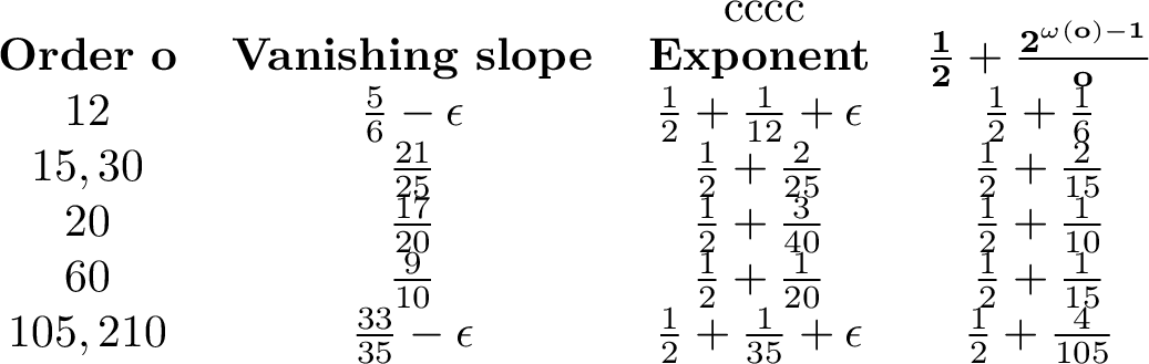
We believe the true exponent should be somewhere between \(\frac{1}{2}+\frac{1}{o}\) and \(\frac{1}{2} +\frac{2^{\omega(o)-1}}{o}\), because of Theorem 5 and the pole of Kubota’s Eisenstein series at \(\frac{1}{2} +\frac{1}{o}\) as mentioned above. As we managed to prove an upper bound of \(\frac{1}{2} +\frac{1}{o}+\epsilon\) when \(o=12\), this leads us to believe that the true exponent is more likely to be \(\frac{1}{2}+\frac{1}{o}\), although we do not have enough evidence to make this a conjecture.

1.2 Application to Möbius and character sums over Galois \(G\)-extensions↩︎

We give another arithmetic application of our technique, this time to Möbius and character sums over \(G\)-extensions of the rational function field \(\mathbb{F}_q(t)\). We set this up following [7]. Let \(G\) be a group and \(R=R_1\sqcup \cdots \sqcup R_n\subseteq G\) be a union of conjugacy classes, and for simplicity we assume that each \(R_i\) is closed under \(q\)-th powering, i.e. \(g\in R_i\Rightarrow g^q\in R_i\). For example, one could simply take \(q\equiv 1\pmod {|G|}\) by Lagrange’s theorem. Define \(\mathcal{E}^{R}_q(G;n_1,\ldots, n_k)\) to be the set of \(G\)-extensions of \(\mathbb{F}_q(t)\) split over \(\infty\), where the sum of degrees of all places with monodromy in \(R_j\) is \(n_j\), and let \(n=n_1+\cdots +n_k\). In addition, we fix an an extension of the infinite place of the function field to its separable closure, which effectively marks a point over \(\infty\) of the corresponding branched cover. Furthermore, denote \(f_L\in \mathbb{F}_q[t]\) to be the conductor of \(L\in \mathcal{E}^{R}_q(G;n_1,\ldots, n_k)\), this is defined to be the radical of the discriminant of \(L\), or alternatively the monic squarefree polynomial with the branch points of \(L/\mathbb{F}_q[t]\) viewed as a branched cover over \(\mathbb{P}^1_{\mathbb{F}_q}\). We refer the reader to [7] for more details.

1.2.1 Möbius function↩︎

Recall that the Möbius function \(\mu(f)\) of a polynomial \(f\in \mathbb{F}_p[t]\) is defined by \(\mu(f)=(-1)^{\omega(f)}\), where \(\omega(f)\) is the number of distinct irreducible factors of \(f\); this is completely analogous to the case over \(\mathbb{Z}\). [7] showed that there is cancellation with a power-savings for the sum of the Möbius function \(\mu(f_L)\) over \(\mathcal{E}^R_q(G;n_1,\ldots, n_k)\) if \(q\) is large enough relative to \(|G|\). This is not surprising because we expect the conductor \(f_L\) to behave randomly. Explicitly, they prove \[\label{eqn:32mobius32es} \left| \sum_{L\in \mathcal{E}^{R}_q(G;n_1,\ldots, n_k)} \mu(f_L)\right | \le 2^{n-1}|R|^nq^{n-\frac{n-d}{2d+4}}\tag{5}\] where \(d=\deg(\bigoplus_{n=0}^\infty H_0(B_n,(\mathbb{C}R)_{-1}))\ge 1\) is finite. Here, \((\mathbb{C}R)_{-1}\) is the relevant braided vector space for this arithmetic problem, and we will define it in Example 1. The bound follows from applying [7] (or equivalently Corollary 1), and as discussed earlier, because of this, the best power-saving exponent they can get is \(\frac{5}{6}\) when \(d=1\).

Instead, we apply Corollary 2 to obtain better exponents for some choices of \(G\) and \(R\) by computing the homology up to \(n\le N\), and we present our results in Figure 6. Note that we can theoretically carry this out for any choice of \(G,R\), but since the computation time is exponential with base \(|R|\), this is more practical for small \(|R|\). The corresponding homological results are obtained in Section 7.2.

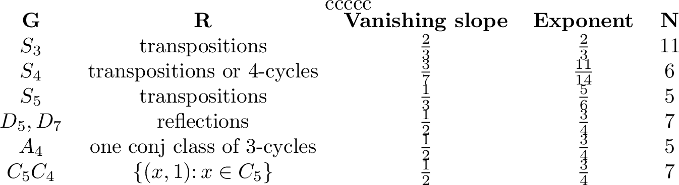
Note that these bounds are not sharp, and computing the homology up to larger and larger values of \(N\) appears to yield progressively stronger bounds. We predict that in most cases the true exponent will be close to \(\frac{1}{2}\), which reflects true randomness of \(f_L\). However, there seems to be some exceptions to this. For example, when \(G=S_4\) and \(R\) is the conjugacy class of transpositions or \(4\)-cycles (these have the same homology as the local systems are isomorphic by [24]), the homology of \((\mathbb{C}R)_{-1}\) seems to have slope \(\frac{1}{2}\) which corresponds to an exponent of \(\frac{3}{4}\), as suggested empirically by Figure 7. Hence, we do not think that a uniform theorem for Möbius sums over all \(G,R\) exists, and the best one can do is to compute for each individual choice of \(G,R\).

1.2.2 Character sums↩︎

Over function fields, if \(q\) is not a power of \(2\), the Möbius function can be written as \(\mu(f)=(-1)^{\deg f}\xi(\mathop{\mathrm{disc}}(f_L))\), where \(\xi\colon \mathbb{F}_q^\times \rightarrow \mathbb{C}^\times\) is the unique quadratic character. This motivates one to consider the sum of \(\chi(\mathop{\mathrm{disc}}(f_L))\) for a general character \(\chi\colon \mathbb{F}_q^\times \rightarrow \mathbb{C}^\times\) instead. Generalizing Equation , [7] prove the bound \[\left| \sum_{L\in \mathcal{E}^{R}_q(G;n_1,\ldots, n_k)} \chi(\mathop{\mathrm{disc}}(f_L))\right | \le 2^{n-1}|R|^nq^{n-\frac{n-d}{2d+4}}\] where \(d=\deg(\bigoplus_{n=0}^\infty H_0(B_n,(\mathbb{C}R)_{\zeta}))\ge 1\) is finite, and \(\zeta\in \mathbb{C}^\times\) is a root of unity of the same order as \(\chi\). Instead, we prove the following bound.

Note that if we fix \(G,R\) and consider the family of sums obtained by varying \(\chi\), the result implies that for any \(\epsilon>0\), all but finitely many characters \(\chi\) have cancellation with exponent smaller than \(\frac{1}{2}+\epsilon\). Indeed, such an almost-all square-root cancellation statement is the best one can hope for because just like in the Möbius case, we do not expect all characters to have close to square-root cancellation. In addition to Figure 7, another example which seems to have smaller power-savings is \(G=S_3\), \(R\) the conjugacy class of transpositions and \(\chi\) a sextic character, which we show in Figure 8. The vanishing slope in this example seems to be \(\frac{1}{3}\) which corresponds to an exponent of \(\frac{5}{6}\). As we can also see from this example, the \(q\)-exponent in the bound is often not optimal, and one can in theory apply Corollary 2 to get better bounds for specific characters.

1.2.3 Multiple characters↩︎

We can also consider the more general situation where we have a product of characters. Let us first fix a choice of \(G,R\). For \(L\in \mathcal{E}^R_q(G;n_1,\ldots, n_k)\), let \(f_{L,i}\) be the monic squarefree polynomial with roots that are branch points with monodromy in \(R_i\). Let \(\chi_i\colon \mathbb{F}_q^\times \rightarrow \mathbb{C}^\times\) for \(1\le i\le k\) and \(\chi_{ij}\colon \mathbb{F}_q^\times \rightarrow \mathbb{C}^\times\) for \(1\le i<j\le k\) be characters, and we consider the sum of \(\prod_{i} \chi_{i} (\mathop{\mathrm{disc}}(f_{L,i}))\prod_{i<j}\chi_{ij}(\mathop{\mathrm{res}}(f_{L,i},f_{L,j}))\) where \(\mathop{\mathrm{res}}(f,g)\) denotes the resultant of the two polynomials \(f,g\). To see why this generalizes our previous scenario, note that when \(\chi_i=\chi\) and \(\chi_{ij}=\chi^2\) the product of characters is simply \(\chi(\mathop{\mathrm{disc}}(f_L))\).

Just like in Theorem 6, we expect that for almost all choices of \(\chi_i,\chi_{ij}\) that there is good cancellation in this sum. It will again be convenient to view these characters as roots of unity, we do this by picking a generator \(a\) of \(\mathbb{F}_q^\times\) and defining \(\zeta_i=\chi_i(a)\), \(\zeta_{ij}^2=\chi_{ij}(a)\) (up to a sign). We choose the convention of \(\zeta_{ij}^2\) because of the identity \(\mathop{\mathrm{disc}}(fg)=\mathop{\mathrm{disc}}(f)\mathop{\mathrm{disc}}(g)\mathop{\mathrm{res}}(f,g)^2\). The space of characters is then parametrized by the torsion points \(((\zeta_i)_i,(\zeta_{ij})_{ij})\in (\mathbb{C}^\times)^{k(k+1)/2}\). Now, consider the example where \(n_1\) is nonzero and \(n_2=\cdots=n_k=0\), here the sum simplifies to the sum in Theorem 6 with \(\chi=\chi_1\) and \(R=R_1\), and as discussed above this may not have good cancellation for some values of \(\chi\). Such a set \(\{\chi_1=b\}\) is a codimension one torsion coset, and one may expect other codimension one torsion cosets to be exceptions to good cancellation. Our theorem shows that we have near square-root cancellation after accounting for these exceptions.

One might notice the resemblance of the condition to the Manin-Mumford theorem for tori, and this is not a coincidence as we use the theorem in our proof. We also obtain one explicit system of equations in Proposition 15.

1.3 Acknowledgments↩︎

I would like to thank my advisor Will Sawin for providing me much valuable guidance along the way. I would also like to thank Jordan Ellenberg, Aaron Landesman, Ishan Levy, David Lin and Mark Shusterman for helpful discussions and feedback.

I acknowledge the use of OpenAI’s GPT-5.5 in generating code used for the computations of homology in this paper, this is discussed in Section 7.4. I take full responsibility for the correctness of the outputs of any AI-generated code. The mathematical content of this paper is my own.

2 Preliminaries↩︎

2.1 Braided vector spaces and shuffle algebras↩︎

Here, we introduce the notions of a braided vector space, quantum shuffle algebra and bar-complex following [5] and [25].

Throughout this paper, we will assume unless otherwise stated that our coefficient field \(k=\mathbb{C}\). We say that a braided vector space \((V,R)\) over \(\mathbb{C}\) is defined over a number field \(K\) if there exists some braided vector space \((V_K,R_K)\) over \(K\) where \(V=V_K\otimes_K C\) and \(R=R_K\otimes_K \mathbb{C}\). Often, we will refer to \((V,R)\) simply as \(V\).

To each braided vector space \(V\), we can associate a quantum shuffle algebra \(\mathfrak A(V)\). Before that, we define the braiding \(R_\sigma\colon V^{\otimes n}\xrightarrow \sim V^{\otimes n}\) attached to a permutation \(\sigma \in S_n\) as follows. Given such a \(\sigma\), there exists a Matsumoto lift \(\tilde{\sigma}\in B_n\) given by expressing \(\sigma\) as the minimum length (reduced) word in transpositions \(s_i=(i,i+1)\) and replacing these with the braid \(\sigma_i\). This lift is well-defined because any two reduced words are related by \(s_is_{i+1}s_i=s_{i+1}s_is_{i+1}\) or \(s_is_j=s_js_i\) for \(|i-j|>1\) which are exactly the braid relations. Then, the braiding \(R_\sigma\) is given by the action of \(\tilde{\sigma}\) on the \(B_n\)-representation \(V^{\otimes n}\).

Now, we define the \(n\)-th bar-cube of \(\mathfrak A=\mathfrak A(V)\) to be the hypercube diagram where vertices are labeled by the \(2^{n-1}\) ordered partitions \([n]\), with the vertex \(\lambda=(\lambda_1,\cdots ,\lambda_k)\) having the term \(\mathfrak A_{\lambda_1}\otimes \cdots \otimes \mathfrak A_{\lambda_k}\), where the edges are given by the shuffle products. For example, for \(n=3\) we have \[\begin{tikzcd}[column sep=large] {\mathfrak A_1\otimes \mathfrak A_1\otimes \mathfrak A_1} & {\mathfrak A_1\otimes \mathfrak A_2} \\ {\mathfrak A_2\otimes \mathfrak A_1} & {\mathfrak A_3.} \arrow["{\mathop{\mathrm{id}}\otimes \tau_{1,1}}", from=1-1, to=1-2] \arrow["{\tau_{1,1}\otimes \mathop{\mathrm{id}}}"', from=1-1, to=2-1] \arrow["{\tau_{1,2}}", from=1-2, to=2-2] \arrow["{\tau_{2,1}}"', from=2-1, to=2-2] \end{tikzcd}\] From the \(n\)-th bar-cube, we can form the \(n\)-th bar-complex \[B_n(\mathfrak A)=\left\{\mathfrak A_1^{\otimes n}\rightarrow \cdots \rightarrow \bigoplus_{\substack{p+q+r=n\\ 0<p,q,r<n}} \mathfrak A_p\otimes \mathfrak A_q \otimes \mathfrak A_r\rightarrow \bigoplus_{\substack{p+q=n\\ 0<p,q<n}} \mathfrak A_p\otimes \mathfrak A_q \rightarrow \mathfrak A_n\right\}\] by collapsing the maps in the bar-cube, and adding a Koszul sign twist so that the differentials of the complex \(d\) satisfy \(d\circ d=0\). The grading of this complex is normalized so that \(\mathfrak A_1^{\otimes n}\) is in degree \(-n\) and \(\mathfrak A_n\) is in degree \(-1\).

The point of introducing quantum shuffle algebras and bar-complexes is to give a way to compute the homology of braided vector spaces: \[\label{eqn:32homology32to32bar-complex} H_i(B_n,V^{\otimes n})^* \cong H^i(B_n,V^{*\otimes n})\cong \mathop{\mathrm{Tor}}^{\mathfrak A(V^*_{-1})}_{n-i,n}(\mathbb{C},\mathbb{C})\cong H^{i-n}(B_n(\mathfrak A(V^*_{-1}))).\tag{6}\] The asterisk here refers to the dual of the corresponding vector space, and \(V_{-1}\) is \(V\) with braiding twisted by a sign as previously defined. The first isomorphism follows from a universal coefficient theorem, the second isomorphism follows from [25] or the dual of [5], and the last isomorphism follows is a general fact that \(\mathop{\mathrm{Tor}}\) can be calculated from the bar-complex. Hence, to show vanishing of \(H_i(B_n,V^{\otimes n})\), it suffices to show that the cohomology of the corresponding bar-complex \(\mathfrak A(V_{-1}^*)\) vanishes in degree \(i-n\).

2.2 Local systems on \(\mathop{\mathrm{Conf}}^n\)↩︎

We define \(\mathop{\mathrm{Conf}}^n\) to be the configuration space of \(n\) distinct unordered points on the affine line \(\mathbb{A}^1\) over \(\mathbb{Z}\). By sending the \(n\) points to the monic polynomial \(f\) with these \(n\) roots, we can identify this with the open subset of \(\mathbb{A}^n\) where the discriminant is invertible. Then, the discriminant gives a morphism \(\delta\colon \mathop{\mathrm{Conf}}^n\rightarrow \mathbb{G}_m\).

The analytification \(\mathop{\mathrm{Conf}}^n(\mathbb{C})\) of the fiber over \(\mathbb{C}\) is the Eilenberg-MacLane space \(K(B_n,1)\). By choosing the basepoint \(c_n=\{1,2,\ldots, n\}\in \mathop{\mathrm{Conf}}^n(\mathbb{C})\), we have the isomorphism \(\pi_1(\mathop{\mathrm{Conf}}^n(\mathbb{C}),c_n)\cong B_n\), where the generator \(\sigma_i\) of the braid group corresponds to the half Dehn twist swapping the points \(i\) and \(i+1\) by moving them counterclockwise around each other.

For non-negative integers \(n_1+\ldots +n_k=n\), we define \(\mathop{\mathrm{Conf}}^{n_1,\ldots, n_k}\) to be the multicolored configuration space of \(n\) distinct points on the affine line with \(n_i\) points of each color. We can view this as a \(k\)-tuple of monic polyomials \((f_1,\ldots, f_k)\) where \(f_i\) has degree \(n_i\). Now, we have \(\pi_1(\mathop{\mathrm{Conf}}^{n_1,\ldots, n_k}(\mathbb{C}),c_n)\cong B_{n_1,\ldots, n_k}\), which is defined to be the subgroup of \(B_n\) which preserves the coloring, i.e. the preimage of \(S_{n_1}\times \cdots \times S_{n_k}\) under the map \(B_n\twoheadrightarrow S_n\). Forgetting the coloring gives a finite étale map \(\tau\colon \mathop{\mathrm{Conf}}^{n_1,\ldots n_k}\rightarrow \mathop{\mathrm{Conf}}^n\). As a special case, define the ordered configuration space \(\mathop{\mathrm{PConf}}^n=\mathop{\mathrm{Conf}}^{1,\ldots, 1}\) where there are \(n\) \(1\)s, then \(\tau\colon \mathop{\mathrm{PConf}}^n\rightarrow \mathop{\mathrm{Conf}}^n\) is a finite étale \(S_n\)-cover.

In the following examples, we recall the construction of three types of local systems over \(\mathop{\mathrm{Conf}}^n\) that were given in [7], together with their trace functions over \(\mathbb{F}_q\) and their analytifications over \(\mathbb{C}\) as \(B_n\)-representations. Let \(l\) be any prime coprime to \(q\) and fix an isomorphism \(\bar \mathbb{Q}_l\cong\mathbb{C}\) which we will implicitly use throughout the paper.

2.3 Arithmetic sums from trace functions↩︎

Now, we discuss how to obtain the desired arithmetic sums in Sections 1.1 and 1.2 from the trace functions of local systems that we discussed previously.

The arithmetic sums in Section 1.2 can be obtained by taking the tensor product of the character sheaves constructed in Example 3 together with the pushforward of the constant sheaf from Hurwitz spaces constructed in Example 4. This is because the trace function of the tensor product of two sheaves is the product of the individual trace functions.

On the other hand, obtaining the bias in Gauss sums as given in Section 1.1 is more complicated. The corresponding trace function is the product of the indicator function for irreducible (prime) polynomials \(\mathbf{1}_{\text{irr}} (f)\), and the Gauss sum \(G_\chi(f)\). We deal with each one as follows.

Firstly, since \(f\in \mathop{\mathrm{Conf}}^n(\mathbb{F}_q)\) is squarefree, [8] tells us that \[\label{eqn:32formula32for32195irr} \mathbf{1}_{\text{irr}} (f) = \frac{1}{n} \sum_{k=0}^{n-1} (-1)^k \mathop{\mathrm{tr}}(\mathop{\mathrm{Frob}}_q,(\mathcal{L}_{\wedge^k \text{std}_n})_{\bar f})\tag{8}\] where \(\mathcal{L}_{\wedge^k \text{std}_n}\) are the local systems constructed in Example 2 corresponding to the \(k\)-th wedge product of the standard representation of \(S_n\).

These representations are direct summands of \(V^{\otimes n}\) for a certain braided vector space \(V=\mathbb{C}_\wedge\). Following [7], we define \(\mathbb{C}_\wedge\) to be the \(2\)-dimensional braided vector space of diagonal type with basis \(\{v_0,v_1\}\) corresponding to the matrix \((q_{ij})=(-1)^{ij}\) as in Example 1(a). Explicitly, the braiding is \[R(v_0\otimes v_0)=v_0\otimes v_0, \;R(v_0\otimes v_1)=v_1\otimes v_0,\;R(v_1\otimes v_0)=v_0\otimes v_1,\;R(v_1\otimes v_1)=-v_1\otimes v_1.\] By [7], we can decompose the \(S_n\)-representation \[\label{eqn:32C95wedge32decomp} \mathbb{C}_\wedge^{\otimes n} = \bigoplus_{k=0}^{n-1} (\wedge^k \text{std}_n)^{\oplus 2},\tag{9}\] so it suffices to look at the braided vector space \(\mathbb{C}_\wedge\) to understand \(\mathcal{L}_{\wedge^k \text{std}_n}\) and \(\mathbf{1}_{\text{irr}}\).

Secondly, we deal with the Gauss sums \(G_\chi(f)\) for a nontrivial multiplicative character \(\chi\colon \mathbb{F}_q^\times \rightarrow \mathbb{C}^\times\), following [20]. Recall that we defined the additive character \(\psi(x)=e^{2\pi i\mathop{\mathrm{tr}}^{\mathbb{F}_p}_{\mathbb{F}_q}x/p}\). Let \(G(\chi,\psi)=\sum_{x\in \mathbb{F}_q^\times} \chi(x)\psi(x)\), which has absolute value \(\sqrt q\) by a property of Gauss sums. Then, taking \(f_1=1\) in [20] and combining with [20] gives for squarefree \(f\) with degree \(n\) that \[\label{eqn:32formula32for32G95chi40f41} G_\chi(f)=(-1)^{n(n-1)(q-1)/4} G(\chi,\psi)^n (\chi\cdot \xi)\left((-1)^{n(n-1)/2}\mathop{\mathrm{disc}}(f)\right)\tag{10}\] where \(\xi\colon \mathbb{F}_q^\times \rightarrow \{\pm 1\}\) is the unique quadratic character and \((\chi\cdot\xi)(x)=\chi(x)\xi(x)\). We see that for fixed \(\chi\), the Gauss sum is basically the character \((\chi\cdot \xi)(\mathop{\mathrm{disc}}(f))\) up to a factor with size \(q^{\deg f/2}\), so we can understand this using the local system \(\delta^* \mathcal{L}_{\chi\cdot \xi}\) in Example 3.

At this point, we could basically deduce the arithmetic bounds in Sections 1.1 and 1.2 assuming the corresponding homological vanishing statements. However, we choose to leave this to Section 8 after we have proven the homological vanishing theorems in the next few sections.

3 Proof of main theorem↩︎

In this section we prove Theorem 1, our main homological vanishing result. The rough idea of the proof is as follows. Suppose we have vanishing for \(H_i(B_n,V^{\otimes n})\) in an \((N,I)\) staircase. Using Equation , this translates to \(H^i(B_n(\mathfrak A))\) vanishing for all \(n\le N\) and \(i\le I-N\), where we let \(\mathfrak A=\mathfrak A(V^*_{-1})\) be the relevant quantum shuffle algebra.

Then, for any \(n>N\), we construct a filtration on the bar-complex \(B_n(\mathfrak A)\). We do this in a combinatorial way – terms in the bar-complex are indexed by partitions, and we determine which filtered piece a term is in based on its corresponding partition. In order to show that the cohomology of the bar-complex vanishes in low degree, it is enough, by a spectral sequence argument, to show this for each graded piece. By our construction, each graded piece of this filtration will be a tensor product of terms like \(\mathfrak A_i\) and \(B_m(\mathfrak A)\) where \(m\le N\). However, by assumption, we know that \(B_m(\mathfrak A)\) vanishes in low degree, and this implies the vanishing of low degree cohomology of each graded piece which completes the proof.

The novelty of our proof lies within the combinatorial construction of the filtration, and to the best of our knowledge nothing similar has been done previously at least in the setting of the bar-complexes.

3.1 A simple example↩︎

To illustrate the idea behind our proof, we look at the simplest example of our theorem, which is when \((N,I)=(2,0)\) and \(n=5\). As mentioned in the introduction (see Corollary 1), the \(I=0\) case is basically the same as [7], so this can also serve as a point of comparison between both proofs. Their proof, as written in [7], uses a spectral sequence argument inspired by [1] which comes from homological algebra.

We now outline our proof in this case. The assumption that \(H_i(B_n,V^{\otimes n})\) vanishes in the \((2,0)\) staircase corresponds to the condition that \(H_0(B_2,V^{\otimes 2})=0\) or equivalently that \(H^{-2}(B_2(\mathfrak A))=0\). In this simple case, since \(B_2(\mathfrak A)\) is the two term complex \(\mathfrak A_1\otimes \mathfrak A_1\rightarrow \mathfrak A_2\) and both terms have the same dimension, we must also have that \(H^{-1}(B_2(\mathfrak A))=0\). However, we will avoid using this fact as it will not be available to us in the general case.

Theorem 1 then claims for \(n=5\) that \(H_0(B_5,V^{\otimes 5})=H_1(B_5,V^{\otimes 5})=0\), so we need to show that \(H^{-5}(B_5(\mathfrak A))=H^{-4}(B_5(\mathfrak A))=0\). We draw the \(5\)-th bar-cube in Figure 9, where for convenience, we write the partition \((\lambda_1,\ldots ,\lambda_k)\) for the term \(\mathfrak A_{\lambda_1}\otimes \cdots \otimes \mathfrak A_{\lambda_k}\).

We consider a four-step filtration on \(B=B_5(\mathfrak A)\) given by \[0=F_0B\subseteq F_1B\subseteq F_2B \subseteq F_3B\subseteq F_4B=B\] where \(F_1B\) consists of all the black terms, \(F_2B\) the red and black terms, and finally \(F_3B\) the red, green and blue terms. By construction, the four graded pieces consists of the blue, green, red and black terms respectively.

Recall that it suffices to show that each graded piece has cohomology only in degree \(\ge -3\). Indeed, from the spectral sequence associated to this filtration \[E_1^{p,q}=H^{p+q}(\mathop{\mathrm{Gr}}_pB)\Rightarrow H^{p+q}(B),\] this would tell us that the \(E^1\)-page only has terms in degree \(\ge -3\), so the abutment only has cohomology in degree \(\ge -3\).

This is immediately true for the black graded piece as it only has terms concentrated in degree \(\ge -3\). The red graded piece is of the form \(B_2(\mathfrak A)\otimes \mathfrak A_2\otimes \mathfrak A_1\) which has terms in degree \(-4\) to \(-3\). The cohomology of this is simply \(H^*(B_2(\mathfrak A))\otimes \mathfrak A_2 \otimes \mathfrak A_1\), where we normalize \(\mathfrak A_i\) to be in degree \(-1\) for each \(i\). Our assumption tells us that \(H^{-2}(B_2(\mathfrak A))=0\), so \(H^{-4}(B_2(\mathfrak A)\otimes \mathfrak A_2\otimes \mathfrak A_1)=0\). Thus, the cohomology of the red graded piece is supported in degree \(\ge -3\). Likewise, the green graded piece is \(\mathfrak A_1\otimes \mathfrak A_2 \otimes B_2(\mathfrak A)\) and by the same argument has cohomology in degree \(\ge -3\). Lastly, the blue graded piece is of the form \(B_2(\mathfrak A)\otimes \mathfrak A_1\otimes B_2(\mathfrak A)\) whose cohomology is \(H^*(B_2(\mathfrak A))\otimes \mathfrak A_1\otimes H^*(B_2(\mathfrak A))\), the first and last terms have cohomology in degree \(\ge -1\) by assumption and the middle term has degree \(-1\), which verifies the claim for the blue graded piece as well. This completes the argument for \(n=5\).

We remark that the filtration described in this section will differ slightly from the one we construct in the next section, since here we have simplified it as much as possible.

3.2 Multi-block filtration↩︎

For the general case, we will need a more complicated filtration which generalizes the one in the previous section. We call this the multi-block filtration because the construction involves breaking \(n\) up into blocks of \(N+1\), and this is where the quasi-periodicity in Theorem 1 comes from.

3.3 Finishing the proof↩︎

We then apply the multi-block filtration to finish the proof of our main theorem.

4 Two methods for homological vanishing↩︎

Let \(V\) be a braided vector space. As mentioned in the introduction, in order to get homological vanishing results in families, we need a uniform way to prove some vanishing staircase of homology. One way to do this, as demonstrated in [7], is to prove vanishing in a minimal \((N,0)\) staircase, which is not difficult as it only requires understanding when \(H^0\) vanishes. In this section, we give two more methods to detect homological vanishing, which can give much stronger vanishing results in families.

4.1 From isomorphisms of shuffle products↩︎

Firstly, we give a necessary and sufficient condition for vanishing in a \((N,N-2)\) staircase in terms of shuffle products of the quantum shuffle algebra. This would then give homological vanishing of slope \(\frac{N-1}{N+1}\) by Theorem 1. Let \(\mathfrak A=\mathfrak A(V^*_{-1})\) be the relevant quantum shuffle algebra for \(V\) by Equation .

The proof will follow the same style as the proof of the main theorem, but it will be much simpler. The crux of the proof is to deduce homological vanishing (b) from some isomorphism of shuffle products (d). The idea is to use a filtration to break up the \(N\)-th bar-cube into various graded pieces, each consisting of two terms connected by an arrow in a fixed direction.

For example, consider the \(4\)-th bar-cube broken down into graded pieces each corresponding to a red vertical arrows in Figure 12. Then, if we knew that \(\tau_{2,2}\colon \mathfrak A_2\otimes \mathfrak A_2\rightarrow \mathfrak A_4\) is an isomorphism, we can conclude by induction on \(N\) that the other graded pieces are also isomorphisms. Indeed, they can be obtained by tensoring \(\tau_{p,q}\colon \mathfrak A_p\otimes \mathfrak A_q\rightarrow \mathfrak A_m\) for \(p+q=m<4\) (which we know are isomorphisms by (c) due to induction) with terms of the form \(\mathfrak A_j\). This tells us that the homology vanishes.

We make this precise in the proof below.

4.2 From the action of the fundamental braid↩︎

Another way to prove homological vanishing of a certain slope is to show that \(H_i(B_n,V^{\otimes n})\) vanishes for all \(i\) for a positive density \(\rho\) of \(n\in \mathbb{N}\). It is not always possible to prove such strong vanishing results, so this technique will only apply for certain cases. This would lead to homological vanishing of slope at least \(\rho\), due to the following corollary of our main theorem.

In words, this is telling us that for every \(n\) where homology doesn’t vanish, there can be at most one more homological degree where homology is non-vanishing.

We remark that we can often get better vanishing results if we use more information on the set \(S\). To see this, consider the toy example where \(S=\{1,10,12,14,\ldots\}\). Then Corollary 3 tells us that this vanishes with slope \(\frac{1}{2}\), but simply applying vanishing in a \((9,7)\) staircase gives \(\frac{4}{5}\) vanishing slope. We will see more examples in Section 7.1 where we use ad-hoc applications of Theorem 1 to get a better bound for individual braided vector spaces.

We will prove such vanishing by looking at the action of the fundamental braid on group cohomology. The fundamental braid is defined to be \(\Delta_n=\prod_{k=1}^{n-1}(\sigma_1\cdots\sigma_{n-k})\) and its square is \(\Delta_n^2=(\sigma_1\cdots\sigma_{n-1})^n\). The center of the braid group \(Z(B_n)\) is cyclic and generated by the square of the fundamental braid \(\Delta_n^2\) when \(n>2\) and the fundamental braid \(\Delta_2\) when \(n=2\) [27]. We have the following proposition.

This will follow from a standard argument in group cohomology. Combined with Corollary 3, this gives us a way to prove vanishing slope in families. We also remark that the statement is also true when \(V^{\otimes n}\) is replaced by another \(B_n\)-representation.

5 Twists of braided vector spaces↩︎

We now study the family of twists of a braided vector space \(V\). In this section, we will study the most general case where there are no assumptions on \(V\), this will by done using the first method of analyzing isomorphisms of shuffle products as in Proposition 9. In the next section, we will study cases where there are additional restrictions imposed on \(V\), which will lead to stronger vanishing results.

Recall that the twist \(V_\zeta\) of \(V\) by \(\zeta\in \mathbb{C}^\times\) is defined by the braiding \(R_{V_\zeta}=\zeta \cdot R_V\). We do not assume that \(\zeta\) is a root of unity. Let \(\mathcal{F}_V\) be the family of all twists of \(V\), and we define \[\mathcal{F}_{V,N}=\{V_\zeta\in \mathcal{F}_V \colon H_i(B_n,V_\zeta^{\otimes n})\text{ vanishes in a }(N,N-2)\text{ staircase}\}.\] We think of this as a “nice set”, as for \(V_\zeta \in \mathcal{F}_{V,N}\), applying Theorem 1 tells us that \(H_i(B_n,V_\zeta^{\otimes n})\) vanishes with slope at least \(\frac{N-1}{N+1}\).

We will prove vanishing in a maximal staircase of \((N,N-2)\) for all but finitely many twists in \(\mathcal{F}_V\), i.e. \(\mathcal{F}_V\setminus \mathcal{F}_{V,N}\) is finite for all \(N\). As a consequence, for any \(\epsilon >0\), all but finitely many twists in \(\mathcal{F}_V\) vanish with slope \(>1-\epsilon\). It turns out that the exceptional twists in \(\mathcal{F}_V\setminus \mathcal{F}_{V,N}\) can be listed from a computation, and we give examples of this in Section 5.2.

5.1 General case↩︎

Let the braided vector space \(V\) have dimension \(d\). We prove the following.

We remark that the size of \(\mathcal{F}_V\setminus \mathcal{F}_{V,N}\) is often much smaller than the bound given above, we will see this in the examples given in Section 5.2. We also note that if \(\zeta\) is a root of unity and \(V\) is defined over \(\mathbb{Q}\), the second statement will tell us that \(\phi(\mathop{\mathrm{ord}}(\zeta))>(N-1)d^N\) implies \(V_\zeta \in \mathcal{F}_{V,N}\).

5.2 Examples↩︎

We now demonstrate how to compute the set of exceptions \(\mathcal{F}_V\setminus \mathcal{F}_{V,N}\) for two examples, which are relevant to the arithmetic situations of character sums over Galois \(G\)-extensions and Gauss sums respectively.

One can compute the following polynomials

\[\begin{align} f_{1,1}(\bar\zeta)&= \Phi_1^2\Phi_2^2,\\ f_{1,2}(\bar\zeta)&=\Phi_1^4\Phi_2^4\Phi_3^2\Phi_6^2,\\ f_{1,3}(\bar\zeta)&=\Phi_1^{12}\Phi_2^{12}\Phi_3^4\Phi_4^4\Phi_6^4,\\ f_{1,4}(\bar\zeta)&= \Phi_1^{24}\Phi_2^{24}\Phi_3^8\Phi_4^8\Phi_5^2\Phi_6^8\Phi_{10}^2\Phi_{20}^2,\\ f_{1,5}(\bar\zeta)&=\Phi_1^{52}\Phi_2^{52}\Phi_3^{22}\Phi_4^{16}\Phi_5^{4}\Phi_6^{22}\Phi_{10}^4 \Phi_{15}^2\Phi_{20}^4\Phi_{30}^2,\\ f_{1,6}(\bar\zeta)&= \Phi_1^{108}\Phi_2^{108}\Phi_3^{44}\Phi_4^{32}\Phi_5^8\Phi_6^{44}\Phi_7^6\Phi_{10}^8\Phi_{14}^6\Phi_{15}^4\Phi_{20}^8\Phi_{21}^2\Phi_{30}^4\Phi_{42}^2,\\ f_{1,7}(\bar\zeta)&= \Phi_1^{224}\Phi_2^{224}\Phi_3^{88}\Phi_4^{72}\Phi_5^{16}\Phi_6^{88}\Phi_7^{16}\Phi_8^8\Phi_{10}^{16}\Phi_{14}^{16}\Phi_{15}^8\Phi_{20}^{16}\Phi_{21}^4\Phi_{28}^4\Phi_{30}^8\Phi_{42}^4\Phi_{56}^4,\\ f_{1,8}(\bar\zeta)&= \Phi_1^{452}\Phi_2^{452}\Phi_3^{182}\Phi_4^{148}\Phi_5^{32}\Phi_6^{182}\Phi_7^{32}\Phi_8^{20}\Phi_9^8\Phi_{10}^{32}\Phi_{12}^6\Phi_{14}^{32}\Phi_{15}^{16}\Phi_{18}^8\Phi_{20}^{32}\Phi_{21}^8\Phi_{24}^6\Phi_{28}^8\Phi_{30}^{16}\Phi_{36}^8\Phi_{42}^8\Phi_{56}^8\Phi_{72}^8, \end{align}\] which gives us the table of of exceptional orders in \(\mathcal{F}_V\setminus \mathcal{F}_{V,N}\) in Figure 15.

We observe from our computation that the exceptional twists \(V_\zeta\in \mathcal{F}_V\setminus \mathcal{F}_{V,N}\) are essentially those whose orders divide some \(n(n-1)\) for some \(n\le N\). This is a phenomenon of \(S_n\)-representations, as we will see in Proposition 12. There is, however, one exception to this when \(N=4\), the twist \(V_\zeta\) with \(\mathop{\mathrm{ord}}(\chi)=12\) is actually in \(\mathcal{F}_{V,4}\). In fact, \(V_\zeta\) lies in \(\mathcal{F}_{V,N}\) for all \(N\le 8\), but not in \(\mathcal{F}_{V,9}\). We will give a more in-depth analysis of this exception in Section 6.2.2.

6 Special cases and extensions for twists↩︎

In this section, we discuss several variants and extensions of the general result, arising under stronger hypotheses on \(V\). In Section 6.1, we study three special cases: finite monodromy, racks coming from groups, and \(S_n\)-representations. We discuss an alternate approach to \(S_n\)-representations via determinantal identities in Section 6.2. Finally, in Section 6.3, we discuss the multicolored generalization where \(V\) is the sum of multiple braided vector spaces and we can introduce twists between each pair of them.

6.1 Finite monodromy, racks and \(S_n\)-representations↩︎

We will consider the following three additional conditions on \(V\).

1. Finite monodromy. For each \(n\), the action of \(B_n\) on \(V^{\otimes n}\) factors through a finite quotient \(H_n\) of \(B_n\). This is typical in most arithmetic settings.

2. Racks from groups. We have \(V=\mathbb{C}R\), where \(R\) is a union of conjugacy classes of a group \(G\). This is relevant to the case of Hurwitz spaces.

3. \(S_n\)-representations. For each \(n\), the action of \(B_n\) on \(V^{\otimes n}\) factors through the symmetric group \(S_n\). This is relevant to \(\mathbb{C}_\wedge\) and irreducibility of polynomials.

Here, (a) is the most general, while (b) and (c) are special cases of (a). That (c) is a sub-case of (a) is obvious by taking \(H_n=S_n\). For (b), \(\mathbb{C}R\) has finite monodromy because the action of \(B_n\) factors through the symmetric group \(S_{|R|^n}\), this is because \(B_n\) acts on the set \(R^n\) of words \(v_1\cdots v_n\) with \(v_i\in R\), and if it acts by the identity permutation on \(R^n\), then it is clear that it also acts by identity on \((\mathbb{C}R)^{\otimes n}\), since \(R^n\) is a basis of this vector space. As in both cases above, it is typical that \(|H_n|\) grows exponentially or super-exponentially.

We obtain results in increasing strength from (a) to (c).

Let us first compare this with the results in the general case in the previous section. When we have one of these additional assumptions (a), (b) or (c), then \(V_\zeta \in \mathcal{F}_V\setminus \mathcal{F}_{V,N}\) only if \(\zeta\) is a root of unity and \(\mathop{\mathrm{ord}}(\zeta)\) satisfies the corresponding divisibility condition for some \(n\le N\). For (b) and (c), there are a lot less of these exceptional twists, and this also explains our observations in Section 5.2. Hence, we can obtain stronger vanishing results by again applying Theorem 1 to the vanishing \((N,N-2)\) staircase.

On the other hand, we can also obtain vanishing results by applying Corollary 3 which tells us that the slope of vanishing is greater than or equals to the density \(\rho\) of \(n\) where homology vanishes. This can be deduced explicitly for the cases of (b) and (c).

As discussed after Corollary 3, this bound on the slope is often not optimal for most \(o\). However, it is a strong uniform statement, which is why we use this for the results stated in the introduction on Gauss sums and character sums. We also remark that for our application to Möbius functions, the relevant braided vector space is twisted by \(-1\) which has order \(o=2\), and this corollary does not give any vanishing in that case.

6.1.1 Proofs↩︎

We now prove Proposition 12 and Corollary 4. Instead of looking at isomorphism of shuffle products like in the previous section, we will instead deduce results from the action of the fundamental braid \(\Delta_n\) as in Proposition 10. The following lemma on \(\Delta_n\) is key.

The proposition now follows from a direct application of Proposition 10.

Finally, we prove the corollary by determining the density \(\rho\) of \(n\in \mathbb{N}\) satisfying the conditions in Proposition 12.

6.2 Aside on determinantal identities↩︎

Let \(V\) satisfy condition (c), that is, each \(V^{\otimes n}\) is an \(S_n\)-representation. We deduced from Proposition 12(c) that \(V_\zeta\in \mathcal{F}_V\setminus \mathcal{F}_{V,N}\) is an exceptional twist only if \(\zeta\) is a root of unity and \(\mathop{\mathrm{ord}}(\zeta)\mid n(n-1)\) for some \(n\le N\).

In this section, we give a separate proof of this fact, which we believe to be rather enlightening and showcases the connection to determinantal identities of Zagier [29] and Hanlon-Stanley [30]. By Proposition 9, it suffices to prove the following statement.

Since \(V^{\otimes n}\) is an \(S_n\)-representation, it follows that the twisted dual \(V_{-1}^{*\otimes n}\) is also an \(S_n\)-representation for all \(n\). Let us view the shuffle product \(\tau^\zeta_{p,q}\colon \mathfrak A^\zeta _p\otimes \mathfrak A^\zeta_q\rightarrow \mathfrak A^\zeta_n\) as a map \(V^{*\otimes n}_{-1}\rightarrow V^{*\otimes n}_{-1}\) via the obvious isomorphisms. Now, by viewing \(V^{*\otimes n}_{-1}\) as a representation of \(S_n\), the map \(\tau^\zeta_{p,q}\) is simply given by the operator \[\Omega_{p,q}(\bar\zeta)=\sum_{\sigma \in \text{Sh}(p,q)} \bar\zeta^{\mathop{\mathrm{inv}}(\sigma)} \sigma \in \mathbb{C}[S_n]\] on this representation.

We want to know for which \(\zeta\) the determinant of the operator \(\Omega_{p,q}(\bar\zeta)\) acting on the representation \(V^{*\otimes n}_{-1}\) is zero. By the representation theory of finite groups, we can decompose the representation \[V^{*\otimes n}_{-1}=\bigoplus_i W_i^{k_i}\] into irreducible representations of \(S_n\). On the other hand, the regular representation \(\mathbb{C}[S_n]\) contains all irreducible representations of \(S_n\). Hence, this means that if \(\Omega_{p,q}(\bar\zeta)\) is invertible on \(\mathbb{C}[S_n]\) then it must be invertible on \(V^{\otimes n}_{-1}\). So Proposition 13 will follow from the following statement.

It turns out that the determinant can be evaluated explicitly using the methods of [29] and [30]. This turns out to be quite elegant and rather tricky. Our argument is based on [30] and [29]. Although some of the statements are already known, we adapt the arguments to give simple and self-contained proofs.

6.2.1 Determinant computations↩︎

We define the operator \[\Omega_n(\bar\zeta)=\sum_{\sigma\in S_n}\bar\zeta^{\mathop{\mathrm{inv}}(\sigma)}\sigma.\] We begin with evaluating the determinant of \(\Omega_{1,n-1}(\bar\zeta)\). This will give us the determinant of \(\Omega_n(\bar\zeta)\) which will in turn give us the determinant of \(\Omega_{p,q}(\bar\zeta)\).

Finally, we have our desired formula, which proves Lemma 4.

6.2.2 An explanation for \(\mathbb{C}_\wedge\) and \(\zeta_{12}\)↩︎

We end the section by briefly explaining the exceptional case of \(\mathop{\mathrm{ord}}(\zeta)=12\) as observed at the end of Example 6. From the previous lemma, we see that the determinant of \(\Omega_{p,q}(\bar\zeta_{12})\) on the regular representation \(\mathbb{C}[S_n]\) is zero for \(n\ge 4\). However, this only implies that \(\Omega_{p,q}(\bar\zeta_{12})\) is degenerate for some irreducible representation \(W_i\). On the other hand, not all irreducible representations of \(S_n\) will appear in \(V^{*\otimes n}_{-1}\) when \(V=\mathbb{C}_\wedge\). In fact, by Equation and [7], \(V^{\otimes n}\) is a direct sum of irreducible representations \(\wedge^k\text{std}_n\), so the irreducible representations in \(V^{*\otimes n}_{-1}\) are simply the dual of these tensored by the sign representation. Hence, it could be possible that \(\Omega_{p,q}(\bar\zeta_{12})\) are non-degenerate on these irreducible representations. We believe that this phenomenon to be a coincidence, and that there are likely no other exceptions for larger \(n\) and \(\mathop{\mathrm{ord}}(\zeta)\).

6.3 Multicolored case↩︎

We now generalize this to the setting of multiple braided vector spaces, which is relevant to applications to multicolored configuration space in Section 1.2.3. Roughly speaking, we want to consider a direct sum decomposition \(V=V_1\oplus\cdots \oplus V_k\), and add twists to the braiding between each \(V_i\) and \(V_j\). We make this precise as follows.

We need to deal with a collection of braided vector spaces with compatible braidings between them, and the following construction makes this possible. Define the notion of a braided monoidal abelian category \((\mathcal{V}, \otimes, 1, R)\) over \(\mathbb{C}\) to be a monoidal \(\mathbb{C}\)-linear abelian category \((\mathcal{V}, \otimes, 1)\) with the following braiding data. For any \(V,W\in \mathcal{V}\), there is a braiding \(R_{V,W}\colon V\otimes W\xrightarrow\sim W\otimes V\) which satisfies the braiding axioms, see [31] Definition 3.2.1.

Let \(\mathcal{V}\) be a braided monoidal abelian category of \(\mathbb{C}\)-vector spaces, which means that the underlying objects of the category are \(\mathbb{C}\)-vector spaces and the tensor product is given by the tensor product as vector spaces. Then, each object \(V\in \mathcal{V}\) is itself a braided vector space by looking at \(R_{V,V}\). This category now admits direct sums by taking the usual direct sum of the underlying vector spaces, with braiding data defined blockwise. The example relevant to our applications is the category of Yetter-Drinfeld modules \(\mathcal{YD}_G\), see [31] or [10] for a definition.

Now, let \(V_1,\ldots, V_k\in \mathcal{V}\) be objects in this category with braiding data \(R_{V_i,V_j}\). We can construct the direct sum \(V=V_1\oplus\cdots\oplus V_k\), and to consider twists of \(V\) we add twists to the braiding data. Let \(\zeta_i\in \mathbb{C}^\times\) for \(1\le i\le k\) and \(\zeta_{ij}\in \mathbb{C}^\times\) for \(1\le i<j\le k\). We can construct another braided monoidal category \(\mathcal{V}'\) which is freely generated by \(V_1',\ldots, V_k'\), where \(V_i'\cong V_i\) are isomorphic as vector spaces but the braiding data is now twisted: \(R_{V_i',V_i'}=\zeta_i\cdot R_{V_i,V_i}\) for \(1\le i\le k\), \(R_{V_i',V_j'}=\zeta_{ij}\cdot R_{V_i,V_j}\) and \(R_{V_j',V_i'}=\zeta_{ij}\cdot R_{V_j,V_i}\) for \(1\le i<j\le k\). This is well defined as the braiding axioms will still be true as the twisting simply introduces a constant multiplier and the required diagrams will commute. Finally, we can define the twist given by the data \(\vec{\zeta}=((\zeta_i)_i,(\zeta_{ij})_{ij})\) to be the braided vector space which is the direct sum \(V_{\vec{\zeta}}=V_1'\oplus\cdots \oplus V_k'\) in the category \(\mathcal{V}'\). We remark that there are other ways to define this, for example, one could follow the definitions in [7].

Let \(\mathcal{F}_V\) be the family of twists \(V_{\vec{\zeta}}\), and \(\mathcal{F}_{V,N}\) be the twists that vanish in a \((N,N-2)\) staircase, defined analogously to Section 5. Recall that these imply vanishing of slope \(\frac{N-1}{N+1}\) by Theorem 1. Without any assumptions on \(V\), we have the following proposition.

Suppose we are only concerned with the case where \(\zeta_i,\zeta_{ij}\) are all roots of unity, like the situation in Section 1.2.3. Then, Manin-Mumford for tori [32] immediately gives us the following corollary.

6.3.1 Additional conditions↩︎

Keeping the assumption that \(\zeta_i,\zeta_{ij}\) are roots of unity, and if we also impose the additional conditions of (a), (b) and (c) in Section 6.1 on \(V\), we can get much more information on these torsion cosets.

We will derive this in an analogous way to Section 6.1. Following the proof of Proposition 12, we choose \(k=2|H_n|\) if \(n\ge 3\) and \(k=|H_2|\) if \(n=2\) for case (a), \(k=2|G|\) for (b) and \(k=2\) for (c). Then, Lemma 3 tells us that \(\Delta_n^k\) acts trivially on \(V^{\otimes n}\). Now, we decompose the \(B_n\)-representation \(V^{\otimes n}\) as \[V^{\otimes n}=\bigoplus_{n_1+\cdots+n_k=n}\mathop{\mathrm{Ind}}_{B_{n_1,\ldots, n_k}}^{B_n}\left(V_1^{\otimes n_1}\otimes \cdots \otimes V_n^{\otimes n_k}\right)\] where the induced representation of the form above is the direct summand of all tensor products which contain the factor \(V_i\) exactly \(n_i\) times. Since \(\Delta_n^k\) acts trivially on \(V^{\otimes n}\), it acts trivially on each of these factors. We decompose \(V_{\vec{\zeta}}^{\otimes n}\) analogously as \[V_{\vec{\zeta}}^{\otimes n}=\bigoplus_{n_1+\cdots+n_k=n}\mathop{\mathrm{Ind}}_{B_{n_1,\ldots, n_k}}^{B_n}\left(V_1'^{\otimes n_1}\otimes \cdots \otimes V_n'^{\otimes n_k}\right),\] so after accounting for the added twists, \(\Delta_n^k\) acts on the twisted induced representation above by \(\vec{\zeta}(n_1,\ldots, n_k)^k\) where we define \[\vec{\zeta}(n_1,\ldots, n_k)\mathrel{\vcenter{:}}=\prod_i\zeta_i^{n_i(n_i-1)/2}\prod_{i<j}\zeta_{ij}^{n_in_j}.\] If this scalar \(\vec{\zeta}(n_1,\ldots, n_k)^k\neq 1\), then the cohomology of the twisted induced representation must be zero by the analogue of Proposition 10 where \(V^{\otimes n}\) is replaced by this representation. Hence, we have the following result in analogy to Proposition 12.

By combining the equations above for \(2\le n\le N\), we have the explicit equations for the torsion cosets in Corollary 5 which cut out the twists in the exceptional set \(\mathcal{F}_V\setminus \mathcal{F}_{V,N}\).

7 Individual braided vector spaces↩︎

In this section, we consider specific examples of braided vector spaces and apply the principle of Corollary 2 to attempt to compute near optimal bounds for each individual braided vector space. We will first look at some twists of \(\mathbb{C}_\wedge\) which are directly related to bias in Gauss sums, then look at sign twists of racks coming from groups \((\mathbb{C}R)_{-1}\) which correspond to Möbius sums over Galois \(G\)-extensions. Lastly, we will consider other examples of braided vector spaces.

7.1 Twists of \(\mathbb{C}_\wedge\)↩︎

Here, we prove the homological vanishing results relevant to Figure 5. We consider \((\mathbb{C}_\wedge)_{\zeta}\) for the following \(5\) cases \(\zeta\in \{\zeta_{12},\zeta_{15},\zeta_{20},\zeta_{60},\zeta_{105}\}\). The point is to showcase how our techniques allow us to prove better bounds given specific orders, and the key is to use the vanishing in Proposition 12(c) to extend the vanishing staircases. In the first three cases, we can get some computational results which will help us get better bounds, and we present this in Figure 16. In the latter two cases, the order is too large for us to observe any \(n\) where the homology does not already vanish trivially by Proposition 12(c). Nevertheless, we can obtain better vanishing results by choosing when to apply Theorem 1 appropriately. We consider each of the \(5\) cases below.

1. \(\zeta_{12}\). Proposition 12(c) tells us that the homology vanishes unless \(n\equiv 0,1,4,9\pmod{12}\), which gives a vanishing slope of \(\frac{2}{3}\) by Corollary 4. From our computations in Figure 16, we see that there is vanishing in a \((8,6)\) staircase, giving a vanishing slope of \(\frac{7}{9}\). We can combine both facts to deduce vanishing in increasingly larger staircases.

   Lemma 8. \(H_i(B_n,(\mathbb{C}_\wedge)_{\zeta_{12}}^{\otimes n})\) vanishes in a \((12 \cdot 2^i-4,10\cdot2^i-4)\) staircase for every \(i\ge 0\).

   Proof. We prove this by induction. The \(i=0\) case of \((8,6)\) is true from above. We now prove the statement for \(i\) assuming that it is true for \(i-1\), i.e. we have vanishing in a \((N,I)\mathrel{\vcenter{:}}= (12\cdot2^{i-1}-4,10\cdot 2^{i-1}-4)\) staircase. Applying Theorem 1 to the \((N,I)=(12 \cdot 2^{i-1}-4,10\cdot2^{i-1}-4)\) staircase tells us that it vanishes for the \((2N+1,2I+1)=(12\cdot 2^i-7,10\cdot 2^i-7)\) staircase. Furthermore, when \(n=12\cdot 2^i-6,12\cdot 2^i-5,12\cdot 2^i-4\), we have \(n\equiv 6,7,8\pmod {12}\) so their homology must vanish by Proposition 12(c). This allows us to extend this to vanishing in a \((12\cdot 2^i-4,10\cdot 2^i-4)\) staircase as desired. ◻

   This lemma gives a vanishing slope of \(\frac{10\cdot 2^i-3}{12\cdot 2^i-3}\), and taking \(i\rightarrow \infty\), the slope of vanishing approaches \(\frac{5}{6}\) as desired.

2. \(\zeta_{15}\). Proposition 12(c) tells us that the homology vanishes unless \(n\equiv 0,1,6,10\pmod{15}\), and Figure 16 tells us that the homology vanishes in a \((15,12)\) staircase. Applying Theorem 1, we deduce vanishing in a \((15\cdot 2 +1,12\cdot 2+1)=(31,25)\) staircase. However, the homology in the range \(32\le n\le 35\) vanishes, so we extend this to the \((35,29)\) staircase. Applying Theorem 1 again, we have vanishing in a \((70,58)\) staircase, and we then extend this to the \((74,62)\) staircase. This gives us vanishing of slope \(\frac{21}{25}\).

3. \(\zeta_{20}\). From Figure 16, we see that there is vanishing in a \((16,13)\) staircase, and Proposition 12(c) extends this to a \((19,16)\) staircase, giving us a vanishing slope of \(\frac{17}{20}\).

4. \(\zeta_{60}\). The homology vanishes unless \(n\equiv 0,1,16,21,25,36,40,45\pmod{60}\). We immediately have vanishing in a \((15,13)\) staircase, giving us a \((15\cdot 2+1,13\cdot 2+1)=(31,27)\) staircase which we extend to \((35,31)\), which further gives \((35\cdot 3+2,31\cdot 3+2)=(107,95)\) and we finally extend this to a \((119,107)\) staircase. This gives us a vanishing slope of \(\frac{9}{10}\).

5. \(\zeta_{105}\). The homology vanishes unless \(n\equiv 0,1,15,21,36,70,85,91\pmod{105}\). By Corollary 3, we have vanishing in a \((69,64)\) staircase. We claim for all \(i\ge 0\) that we have vanishing in a \((105\cdot 2^i-36,99\cdot 2^i-35)\) staircase, and prove this by induction as follows. The base case is true, and if we have vanishing for \((N,I)=(105\cdot 2^{i-1}-36,99\cdot 2^{i-1}-35)\), we have vanishing for \((2N+1,2I+1)=(105\cdot 2^i-71,99\cdot 2^i-69)\). There is only one possible \(n\) with nonzero homology in the range \(105\cdot 2^i-70\le n\le 105\cdot 2^i-36\), so by the proof of Corollary 3 this results in at most one more homological degree where homology could be nonzero. Hence, we have vanishing for \((2N+1+35, 2I+1+34)=(105\cdot 2^i-36, 99\cdot 2^i-35)\) as desired. This gives us a slope of vanishing that approaches \(\frac{33}{35}\) as \(i\rightarrow \infty\).

7.2 Sign twist of \(\mathbb{C}R\)↩︎

We now consider some examples of the braided vector spaces \((\mathbb{C}R)_{-1}\) where \(R\) is a union of conjugacy classes in a group \(G\), focusing on the cases in Figure 6. Unlike the previous section which discusses twists of \(\mathbb{C}_\wedge\), we do not have strong vanishing results coming from Proposition 12. Indeed, as remarked earlier, since \(\mathop{\mathrm{ord}}(-1)=2\), the divisibility condition \(\mathop{\mathrm{ord}}(\zeta)\mid n(n-1)|G|\) in Proposition 12(b) is trivially satisfied, so it does not give us any vanishing \(n\). This is actually the truth, as we will see in the examples below. Because of this, we are only able to prove vanishing slopes by computing homology for small \(n\). We present our computations in Figure 17. The example of \(G=S_4\) and \(R\) the conjugacy class of transpositions was already given in Figure 7. By applying Theorem 1 to the appropriate vanishing staircases indicated, we get the desired slopes of vanishing in Figure 6.

7.3 Other braided vector spaces↩︎

Lastly, we consider other braided vector spaces which may not necessarily correspond to something arithmetic. These examples are usually connected to physics because braided vector spaces are solutions to the Yang-Baxter equation.

First, we look at Gaussian braided vector spaces \(V\) of dimension \(m\) as defined in [33]. Let \(\zeta=\zeta_m\) if \(m\) is odd and \(\zeta=\zeta_{2m}\) if \(m\) is even. Let \(\{e_1,\ldots, e_m\}\) be a basis of \(V\), and define the braiding by \[R(e_i\otimes e_j)=\frac{1}{\sqrt m}\sum_{k=0}^{m-1}\zeta^{k^2+{k(j-i)}}e_{i+k}\otimes e_{j+k}.\] As an example, we compute the homology for the three-dimensional Gaussian braided vector space in Figure 18, and we from this we see a vanishing slope of \(\frac{5}{7}\).

Next, we look at two dimensional braided vector spaces, which were classified completely in [34]. The classification organizes the solutions according to the number of free parameters and the rank of the braiding. We choose to look at the solutions with no free parameters, since these are in some sense the most canonical. We also require them to be of full rank as in our case we require \(R_{V,V}\colon V\otimes V\xrightarrow\sim V\otimes V\) to be an isomorphism. Then, there are three solutions, with braiding matrix written as follows with respect to the basis \(e_1\otimes e_1,e_1\otimes e_2,e_2\otimes e_1,e_2\otimes e_2\): \[R_1=\begin{pmatrix} 1 & & &1\\ & &-1& \\ &-1& & \\ & & &1 \end{pmatrix},\;R_2=\frac{1}{\sqrt 2}\begin{pmatrix} 1 & & &1\\ &1&1& \\ &-1&1& \\ -1& & &1 \end{pmatrix},\;R_3=\begin{pmatrix} 1 & & &\\ & 1&& \\ & & 1& \\ & & &1 \end{pmatrix}.\]

Note that the convention of the braiding matrix here differs from that in [34] by swapping the second and third columns. We also normalize \(R_2\) by dividing by \(\sqrt 2\) so the eigenvalues have absolute value \(1\).

Let \(V_i\) be the two-dimensional braided vector space with braiding \(R_i\). The case of \(V_3\) is not interesting as the braiding \(R_3\) is trivial and \(B_n\) acts trivially on \(V_3^{\otimes n}\). In this case the homology can be deduced from the classical computation of the homology of configuration space and is simply \(H_i(B_n,V_3^{\otimes n})=V_3^{\otimes n}\) for \(0\le i\le \min(n-1,1)\) and \(0\) otherwise.

For \(V_1\), we can consider all twists \((V_1)_\zeta\) by some \(\zeta\in \mathbb{C}^\times\), and recall that this corresponds to multiplying \(R_1\) by \(\zeta\). It is not hard to see that if \(1\) is not an eigenvalue of \(\zeta R_1\), then \(H_0(B_2,(V_1)_\zeta^{\otimes 2})=H_1(B_2,(V_1)_\zeta^{\otimes 2})=0\) and so the homology vanishes with slope at least \(\frac{1}{3}\). We now consider the case when \(1\) is an eigenvalue, which forces \(\zeta=1\) or \(\zeta=-1\). We compute the homology in Figure 19. We see that \(V_1\) itself seems to exhibit homological stability, while the twist \((V_1)_{-1}\) vanishes with slope at least \(\frac{6}{11}\).

Finally, one can check that \(V_2\) is actually isomorphic to the two-dimensional Gaussian braided vector space via a change of basis. We compute that the homology of \(V_2\) itself vanishes for \(2\le n\le 13\), and we are not sure whether the homology actually vanishes for all \(n\ge 2\). Using the same reasoning as above, we see that all twists \((V_2)_\zeta\) vanish with slope at least \(\frac{1}{3}\) unless \(\zeta=\zeta_8\) or \(\zeta=\bar\zeta_8\). Since these two are complex conjugates, they have the same homology, which we compute in Figure 20. We observe that there is homological vanishing of slope \(\frac{1}{4}\) which seems to be sharp. Furthermore, all dimensions of homology are powers of \(2\), and there appears to be an underlying pattern which also resembles the three-dimensional Gaussian braided vector space.

7.4 Homological computations and algorithms↩︎

The homology \(H_i(B_n,V^{\otimes n})\) can be computed explicitly from the bar-complex as seen in Equation . Hence, in order to compute the dimensions of homology, it suffices to compute the rank of the differentials in the bar-complex. This is not difficult as one can easily write explicit matrices for the differentials from the definition of the shuffle product. Hence, most of the work comes from optimizing the computation of rank of these matrices so that one can improve the range of computation for \(n\).

Recall that if \(V\) is a braided vector space of dimension \(d\), the largest term in the bar-complex has dimension \(D\approx \binom n {\lfloor n/2\rfloor} d^n = O((2d)^n)\), so the largest differentials have dimensions of this size. A simple Gaussian elimination algorithm would take \(O(D^3)\) time and becomes infeasible quickly.

The key improvement comes from the realization that the matrices corresponding to the differentials in the bar-complex are sparse. Let \(z\) be the number of non-zero entries in each row, which is much smaller than \(D\). A typical example in our case (say \(V=\mathbb{C}R\) for \(R\) the rack of transpositions in \(S_3\) and \(n=10\)) could have \(D\approx 10^{7}\) and \(z\approx 100\). We use the block Wiedemann algorithm [35]–[37] which is a probabilistic algorithm that computes the kernel vectors (and hence the rank) of a matrix over \(\mathbb{F}_p\), which has complexity \(O(D^2z)\), which for our applications saves a factor of \(\approx 10^5\), although the larger constant overhead reduces this factor somewhat. To get a matrix over a finite field, we randomly chose a few large primes \(p\) and reduce our matrix modulo \(p\), checking that the rank in the same for each prime.

A smaller improvement to the algorithm is to note that the differential preserves certain invariants like the global monodromy for the case of racks from groups, allowing us to decompose the matrix for the differential into smaller blocks and running the algorithm on each of them.

We believe that there could be a faster algorithm by exploiting the spectral sequences associated to filtrations similar to those in Section 3. We attempted to implemented this but failed.

We prompted GPT-5.5 to implement the algorithm described above in C++. We did this in several steps, by first asking it to implement the simpler Gaussian elimination algorithm, then changing this to the block Wiedemann algorithm while keeping in mind complexity constraints, and implementing a multi-threaded version. We then asked it to optimize the code for speed as much as possible. We also did manual profiling of the code to see which parts took the most time and suggested changes to GPT-5.5. We verified correctness of the output in a variety of test cases at each step. The AI-generated code is available here.

8 Proof of arithmetic statements↩︎

Finally, we link the homological results in the previous few sections to our arithmetic applications as stated in Section 1.1 and 1.2.

8.1 Möbius and character sums↩︎

We first tackle the case of the Möbius function and character sums as it is slightly simpler. We will prove Theorem 6 and 7 and justify Figure 6. We remark that this is rather similar to [7] because we are in the same arithmetic situation.

Recall that the Möbius function is the special case when \(\chi=\xi\) is the quadratic character, so the above proof tells us that a vanishing slope of \(B\) for \((\mathbb{C}R)_{-1}\) leads to a \(q\)-exponent of the form \((1-\frac{B}{2})n+C\). Hence, the computations in Figure 7 and 17 justifies Figure 6.

We now deal with the statement for multiple characters.

8.2 Bias in Gauss sums↩︎

We now prove Theorem 3 and 5 as well as justify Figure 5.

Similarly, from the same argument above, one can prove the \(q\)-exponents in Figure 5 using the computations in Section 7.1.

References↩︎