Embedding Foundation Model Predictions
in Discrete-Choice Models with Structural Guarantees
June 24, 2026
Abstract
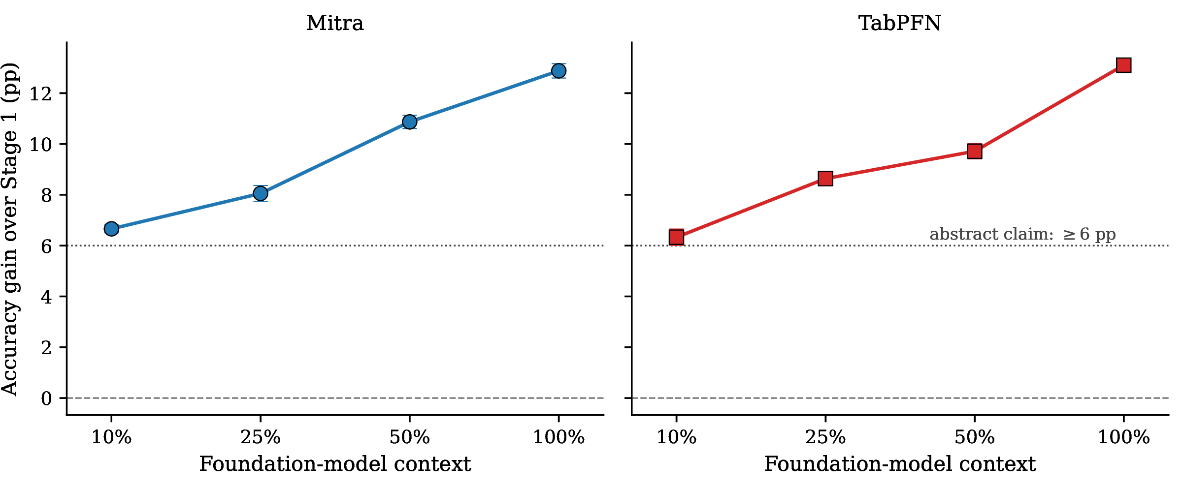
Tabular foundation models achieve strong accuracy on choice prediction tasks, but their predictions often violate the economic logic those tasks require: raising a price can increase predicted demand, implied willingness-to-pay estimates are frequently negative or implausible, and unavailable alternatives receive nonzero probability. We propose a two-stage adapter that takes a foundation model’s predicted choice probabilities as a precomputed feature and embeds them inside a multinomial logit’s utility. In Stage 1, we fit the multinomial logit’s structural coefficients by maximum likelihood with sign constraints; in Stage 2, we freeze those coefficients and fit a small neural correction operating on the foundation model’s predictions. We prove that this composition exactly preserves the multinomial logit’s marginal rate of substitution, so analytically computable value-of-time becomes a mathematical guarantee rather than an empirical accident. Across three datasets and two foundation models, the adapter gains 6.4 percentage points (pp) of test accuracy on average over the multinomial logit and up to 12.8 pp, maintains 100% cost monotonicity, and produces values of time within the published transportation-economics range on the transportation datasets. Performance degrades gracefully under foundation-model context restriction, retaining at least 6 pp of accuracy gain even at 10% of the original foundation-model context.
1 Introduction↩︎
Discrete-choice models guide policy decisions with significant economic stakes: the per-minute value of time from commuter mode-choice forecasts [1], [2] anchors cost-benefit appraisal of multi-billion-dollar rail and road investments, and willingness-to-pay estimates from consumer discrete-choice experiments set prices and predict how labeling regimes shift behavior. A choice model must do two things: forecast which alternative is chosen, and forecast how the choice responds to intervention.
Multinomial-logit utility models [1], [2] satisfy the second requirement by construction: a sign-constrained cost coefficient gives monotone demand, the \(\beta_{\text{time}}/\beta_{\text{cost}}\) ratio gives interpretable willingness-to-pay, and unavailable alternatives receive zero probability. They satisfy the first only modestly. Modern machine-learning models invert the trade-off, raising accuracy at the cost of breaking each structural property in turn [3]–[5].
Tabular foundation models such as TabPFN [6], [7] and Mitra [8] intensify the tension by raising the accuracy ceiling while inheriting the same structural failures. Existing remedies each carry costs: architecturally constrained monotonic neural networks [9]–[11] eliminate monotonicity violations but lose the closed-form trade-off ratio; knowledge distillation [12] into a multinomial-logit student preserves the structural guarantees but cannot match the teacher’s accuracy; penalized fine-tuning needs gradient access through the foundation model’s weights, incompatible with the in-context learning that TabPFN and Mitra use at inference.
We propose a two-stage adapter that embeds the foundation model’s predicted probability vector inside a constrained multinomial logit as a precomputed feature. In Stage 1, we fit the structural coefficients by maximum likelihood under the usual MNL constraints with the correction held at zero; in Stage 2, we freeze those coefficients and fit a small neural correction. We prove that this two-stage procedure preserves the structural marginal rate of substitution exactly, and that joint training of the structural coefficients and the correction does not: correction expressivity creates a one-parameter family of likelihood-equivalent solutions, breaking identifiability.
Our contributions are:
A two-stage behavioral adapter that preserves the structural multinomial logit’s economic guarantees by construction while recovering most of a foundation model’s accuracy advantage.
Propositions 1 and 2 identify two-stage training as the design choice preserving structural identifiability and characterize the failure mode of joint training.
Three discrete-choice datasets, two foundation models, six ablations, a feature-augmented multinomial-logit baseline, calibration analysis with three post-hoc methods, and a counterfactual aggregate-share evaluation. The accuracy gain is positive in \(10\) of \(10\) bootstrap replicates on every (dataset, foundation-model) cell, with \(p \approx 0.002\) under the exact binomial sign test and McNemar paired-observation \(p\)-values below \(10^{-20}\) on the larger datasets.
A behavioral-audit recipe applicable to any discrete-choice dataset and any predict-function, generalizing value-of-time auditing to willingness-to-pay for arbitrary non-cost attributes and to cluster-aware aggregation for panel data.
2 Related work↩︎
2.0.0.1 Machine learning and economic consistency in choice modeling.
Discrete-choice modeling has been the standard tool in transportation economics and consumer behavior since [1]. Recent work pushes machine learning into the field while exposing a tension with economic structure: [3] document consistent accuracy gains across neural and ensemble methods over the multinomial logit but few behavioral diagnostics; [5] report frequent monotonicity violations and implausible willingness-to-pay estimates from machine-learning choice models; and [4] frame economic consistency as an open challenge distinct from prediction accuracy. [13] (TasteNet) propose a neural-embedded discrete-choice model that learns taste parameters as neural-network functions of individual characteristics, targeting taste-parameter interpretability through learned heterogeneity rather than the structural-plus-correction decomposition we adopt here. This work builds on our workshop paper [14]; the present paper extends it with an additional dataset, formal preservation results, and counterfactual aggregate-share evaluation. Our work additionally derives a formal preservation result, evaluates across foundation models, and characterizes joint training’s failure mode.
2.0.0.2 Architecturally constrained monotonic neural networks.
Architectural approaches enforce monotonicity through sign-constrained weights and monotone activations [9]–[11], eliminating cost-monotonicity violations but losing the closed-form trade-off ratio: with no global coefficients, the value-of-time analogue must be computed from per-observation gradients rather than read off as \(\beta_{\text{time}} / \beta_{\text{cost}}\). Our adapter takes a different point: monotonicity and trade-off ratios come from the structural component, whose constrained parameterization is preserved throughout training, while the foundation model contributes a non-differentiable side channel.
2.0.0.3 Tabular foundation models and knowledge distillation.
Tabular foundation models such as TabPFN [6], [7] and Mitra [8] achieve strong classification accuracy via in-context learning. Their published benchmarks emphasize predictive accuracy; structural-validity diagnostics specific to choice modeling (cost-monotone responses, finite positive trade-off ratios, zero probability on unavailable alternatives) at test-row coverage are not part of these benchmarks. Our audit fills this gap. Knowledge distillation [12] into a multinomial-logit student preserves structural guarantees but is bounded by the student’s expressive capacity: a plain MNL student parameterizes a strictly linear-in-features utility, and the residual variance the foundation model captures lives above that ceiling. We position the foundation model differently: its predictions become an explanatory feature embedded inside a structurally constrained utility, with the foundation model’s parameters never modified.
3 Method↩︎
3.1 Setup and notation↩︎
We consider a discrete-choice setting with \(N\) observations indexed by \(i \in \{1, \dots, N\}\). Each observation has a feature vector \(\mathbf{x}_i \in \mathcal{X}\), a set of available alternatives \(\mathcal{K}_i \subseteq \{1, \dots, K\}\), and an observed choice \(y_i \in \mathcal{K}_i\). For panel data we additionally observe a subject identifier \(s_i\), since multiple observations from the same subject are not exchangeable; we cluster on \(s_i\) throughout.
A choice model produces probabilities \(P_k(\mathbf{x}_i) \in [0, 1]\) summing to one over \(\mathcal{K}_i\), i.e., a vector on the \((K{-}1)\)-simplex \(\Delta^{K-1}\). The standard multinomial logit (MNL) parameterizes these through a linear utility \(V_k(\mathbf{x}_i) = \boldsymbol{\beta}^\top \boldsymbol{\phi}_k(\mathbf{x}_i)\) and the softmax \(P_k = \exp V_k / \sum_{j \in \mathcal{K}_i} \exp V_j\) [1]. The alternative-specific feature transform \(\boldsymbol{\phi}_k\) selects from \(\mathbf{x}_i\) the columns that enter alternative \(k\)’s utility, typically including cost, time, alternative-specific constants, and sociodemographic interactions. We treat \(\boldsymbol{\phi}_k\) as fixed by the dataset’s specification and recover \(\boldsymbol{\beta}\) by maximum likelihood.
3.2 Behavioral audit↩︎
Every model is evaluated through three model-agnostic functionals that take only a predict function \(\mathbf{x} \mapsto P(\mathbf{x}) \in \Delta^{K-1}\) as input. We say model-agnostic in the sense that the audit reads model outputs only, requiring no gradient access or knowledge of internals.
Intervention protocol. For adapter and feature-augmented MNL we use the fixed-\(\mathbf{q}\) protocol throughout: when a cost or attribute is perturbed at row \(i\), the foundation-model probability vector \(\mathbf{q}_i\) is held fixed at the value computed on the unperturbed \(\mathbf{x}_i\), and the perturbation enters only \(V^{\text{struct}}_k\). The alternative recomputed-\(\mathbf{q}\) protocol re-runs the foundation model on perturbed inputs; we use it for the raw foundation-model counterfactual evaluation (Section 5.3) only, and forfeit the structural guarantees in that case.
The three functionals are: (1) Monotonicity. For each test row \(i\) and alternative \(k\), perturb \(k\)’s cost upward by \(1\%\) of its observed range and check whether \(P_k\) falls; we report the observation-level rate (cluster-aware on panel data). (2) Trade-off ratio. The marginal rate of substitution between non-cost attribute \(a\) and cost \(b\), reported in the standard transportation-economics sign convention so that value of time and willingness to pay for utility-improving attributes are positive: \(\rho^{\mathrm{VOT}}_{a,b} = (\partial P_k/\partial a) / (\partial P_k/\partial b)\) when both partials are negative (e.g., time and cost both lower utility), and \(\rho^{\mathrm{WTP}}_{a,b} = -(\partial P_k/\partial a) / (\partial P_k/\partial b)\) when \(\partial P_k/\partial a\) is positive and \(\partial P_k/\partial b\) is negative (a desirable non-cost attribute vs cost). Estimated by finite differences scaled to \(1\%\) of each column’s observed range. (3) Availability compliance. For datasets in which the available set \(\mathcal{K}_i\) varies across observations (e.g., Swissmetro, where the proposed Swissmetro option is not offered to some respondents), \(\mathrm{Leak}(M) = \mathbb{E}_i [\sum_{k \notin \mathcal{K}_i} P_k(\mathbf{x}_i)]\) measures the predicted probability assigned to formally unavailable alternatives. The multinomial logit applies softmax over \(\mathcal{K}_i\) only, so its leak is mechanically zero; black-box predictors that ignore the availability mask can leak nonzero probability onto unavailable alternatives.
3.3 Two-stage behavioral adapter↩︎
For each observation \(i\), alternative \(k\), and a precomputed foundation-model probability vector \(\mathbf{q}(\mathbf{x}_i) \in \Delta^{K-1}\) obtained by a single forward pass through the foundation model on the raw input, the adapter’s utility is \[V_k(\mathbf{x}_i) = \underbrace{\boldsymbol{\beta}^\top \boldsymbol{\phi}_k(\mathbf{x}_i)}_{V_k^{\text{struct}}\text{ (economic structure)}} + \underbrace{g_k(\mathbf{q}(\mathbf{x}_i))}_{\text{foundation-model correction}}, \label{eq:adapter}\tag{1}\] where \(g \colon \Delta^{K-1} \to \mathbb{R}^K\) is a small MLP (two hidden layers, width \(32\)). To enforce cost/time monotonicity throughout training we reparameterize each such coefficient as \(\beta = -\exp(\theta)\).
We fit the model in two sequential stages. Stage 1: with the correction held at \(g \equiv 0\), fit \(\boldsymbol{\beta}\) by maximum likelihood under the sign constraints, recovering the standalone-MNL estimate \(\boldsymbol{\beta}^\ast\). Stage 2: fix \(\boldsymbol{\beta} = \boldsymbol{\beta}^\ast\) and fit only \(g\) by maximum likelihood. The architecture realizes Stage 1 cleanly because \(g\)’s output layer is zero-initialized; hidden weights use He initialization [15]. Because \(\mathbf{q}(\mathbf{x}_i)\) is precomputed, \(\partial \mathbf{q}/\partial \mathbf{x}_i = 0\), so monotonicity and trade-off ratios reduce to functions of \(\boldsymbol{\beta}^\ast\) alone. Propositions 1–2 make this precise and identify joint training as the failure mode.
3.4 Propositions↩︎
We use \(\boldsymbol{\beta}^\ast\) for the Stage 1 maximum-likelihood estimate and reuse the notation of 1 .
Proposition 1 (Marginal-rate-of-substitution preservation under two-stage training, fixed-\(\mathbf{q}\) protocol). Let \(\boldsymbol{\beta}^\ast\) be the Stage 1 maximum-likelihood estimate, let \(g\) be any Stage 2 parameters in 1 , and operate under the fixed-\(\mathbf{q}\) protocol of Section 3.2. For any two attributes \(j, j'\) that enter the model only through \(V^{\text{struct}}_k(\mathbf{x}_i) = \boldsymbol{\beta}^\top \boldsymbol{\phi}_k(\mathbf{x}_i)\), and for any \(\mathbf{x}_i\) at which \(\boldsymbol{\phi}_k\) is differentiable in \(x_{ij}\) and \(x_{ij'}\), \[\mathrm{MRS}_{j,j'}(\mathbf{x}_i) \;\equiv\; \frac{\partial V_k(\mathbf{x}_i) / \partial x_{ij}}{\partial V_k(\mathbf{x}_i) / \partial x_{ij'}} \;=\; \frac{\beta^\ast_j}{\beta^\ast_{j'}}.\] In particular, the value-of-time analogue \(\beta^\ast_{\text{time}} / \beta^\ast_{\text{cost}}\) is identical to the standalone multinomial logit’s value-of-time and is invariant to the choice of foundation model and to the choice of \(g\). Under the recomputed-\(\mathbf{q}\) protocol, \(g\) contributes a chain-rule term through \(\mathbf{q}\) to each partial and the ratio no longer reduces to \(\beta^\ast_j / \beta^\ast_{j'}\) in general.
Corollary (probability-derivative MRS). Under the same fixed-\(\mathbf{q}\) protocol, restrict attention to attributes \(j, j'\) that enter only alternative \(k\)’s utility. Then the audit estimator equals the structural coefficient ratio under the audit’s sign convention: \(\rho^{\mathrm{VOT}}_{j,j'} (\mathbf{x}_i) = \beta^\ast_j / \beta^\ast_{j'}\) and \(\rho^{\mathrm{WTP}}_{j,j'}(\mathbf{x}_i) = -\beta^\ast_j / \beta^\ast_{j'}\), since the softmax derivative’s \(P_k(1-P_k)\) factor cancels in the ratio (Appendix 9.1).
Intuition. Fixed \(\mathbf{q}\) forces \(\partial \mathbf{q}/\partial \mathbf{x} = 0\), so \(g\) vanishes from \(\partial V_k / \partial x_{ij}\) and the ratio collapses to \(\beta^\ast_j / \beta^\ast_{j'}\). Full proof in Appendix 9.1.
Proposition 2 (Joint training breaks structural identifiability). Assume there exists a continuous \(\kappa_k: \Delta^{K-1} \to \mathbb{R}\) such that \(\mathrm{cost}_k(\mathbf{x}) = \kappa_k(\mathbf{q}(\mathbf{x}))\) on the closure of the training support (cost-recoverability assumption); the correction class \(\mathcal{G}\) is dense in \(C^0(\Delta^{K-1}, \mathbb{R}^K)\) [16]; and \(L(\boldsymbol{\beta}, g)\) is minimized jointly without two-stage constraints. Then for any joint minimizer \((\boldsymbol{\beta}^{(0)}, g^{(0)})\) there exists a one-parameter family \(\{(\boldsymbol{\beta}^{(c)}, g^{(c)}) : c \in \mathcal{C}\}\) of distinct configurations achieving identical loss, parametrized by \(\beta^{(c)}_{\text{cost}} = \beta^{(0)}_{\text{cost}} + c\) for \(c\) in an open interval \(\mathcal{C}\) preserving sign constraints on \(\beta_{\text{cost}}\). Gradient descent within \(\mathcal{C}\) selects an initialization-dependent point rather than the MNL MLE \(\boldsymbol{\beta}^\ast\).
Note (cost-recoverability). The assumption is dataset-dependent; partial-recoverability cases in Appendix 10.1.
Intuition. Subtracting \(c \cdot \kappa_k(\mathbf{q})\) from \(g_k\) shifts \(\beta_{\text{cost}}\) by \(+c\) without changing pointwise utility: the structural increase \(c \cdot \mathrm{cost}_k\) in \(V_k\) is cancelled by the correction-side decrease. A3 (§6) is the empirical illustration; full proof in Appendix 9.2.
4 Experimental setup↩︎
4.0.0.1 Datasets.
We evaluate on three discrete-choice datasets. Swissmetro [17]: \(10{,}719\) stated-preference commuter choices among rail, the proposed Swissmetro, and car. LPMC [18]: \(81{,}086\) revealed-preference London trips among walk, cycle, public transport, and drive. IoT-Wearables [19]: \(6{,}362\) stated-preference choices among three Internet-of-Things wearable devices varying in price, functional features, and a security/privacy labeling scheme (panel data, \(728\) subjects). All splits are \(70/15/15\). IoT-Wearables uses subject-level splitting (each subject’s rows go entirely to one split) to prevent within-subject leakage. Swissmetro and LPMC use the stratified row-level splits inherited from prior released parquets ([17] for Swissmetro and the LPMC public release); because Swissmetro is stated-preference with repeated choice tasks per respondent, row-level splitting may leak respondent-specific preferences across train/val/test, which we flag as a limitation.
4.0.0.2 Foundation-model inputs.
The foundation-model input columns per dataset:
Swissmetro: per-alternative travel time, cost, headway, availability indicators; respondent age, income, season-ticket holding, luggage, trip purpose.
LPMC: per-alternative duration, transit and driving costs, trip distance; respondent age, sex, license, car ownership.
IoT-Wearables: per-alternative price, functional features, security label; respondent age, education, sex, security-behavior score, condition fixed effects.
Cost (or price), time (or duration), and availability indicators are therefore in the input set on every dataset; this is the basis for the foundation model’s potential non-monotonic response to cost, and motivates the fixed-\(\mathbf{q}\) intervention protocol of Section 3.2 for the adapter.
4.0.0.3 Models.
Each cell evaluates five primary models, reported in Table 1:
Multinomial logit (Stage 1 of the adapter).
Architecturally constrained monotonic neural network [11].
Feature-augmented multinomial logit, with \(\mathbf{q}\) appended to the structural feature set.
Simplified two-stage adapter \(V_k = V^{\text{struct}}_k + g_k(\mathbf{q})\).
Three additional variants appear in prose only: a masked foundation model (Swissmetro, §5.1); a convex ensemble \(\alpha P_{\text{MNL}} + (1{-}\alpha) P_{\text{FM}}\) (§5.2); and the two-term variant \(V_k = V^{\text{struct}}_k + \alpha \log q_k + g_k(\mathbf{q})\) (ablation A2). The correction network \(g\) is a two-hidden-layer MLP, width \(32\), output-layer-zero initialization (§3.3).
4.0.0.4 Foundation-model context and cross-fitted training \(\mathbf{q}_i\).
Stage 2’s training-row \(\mathbf{q}_i\) come from a \(k=5\) stratified cross-fitted protocol, so no row’s prediction was made by a model that saw its own label; test \(\mathbf{q}_i\) are out-of-context by construction. The protocol applies to five of six (dataset, FM) cells; TabPFN-LPMC exceeds the CUDA attention-kernel ceiling at LPMC’s per-fold context size and retains in-sample \(\mathbf{q}_i\) (marked with \(^{\dagger}\) in Table 1). Cross-fitting shifts adapter test accuracy by at most \(-0.6\) pp (Appendix 13).
4.0.0.5 Metrics and significance.
We report:
Test-set accuracy.
Per-row monotonicity rate (cluster-aware aggregation on IoT-Wearables).
Trade-off ratio: value-of-time on transportation datasets; willingness-to-pay for indicated non-cost attributes on IoT-Wearables.
Availability leak (Swissmetro only).
Expected calibration error (ECE), post-calibration with \(K=15\) equal-weight bins.
For each (dataset, foundation-model) cell we draw \(10\) bootstrap samples of the training set with replacement and refit Stage 1 and Stage 2 independently on each replicate; validation and test splits are held fixed. Significance tests on the per-seed accuracy gain (full adapter \(-\) Stage 1) include an exact two-sided binomial sign test (\(p \approx 0.002\) at \(10/10\) positive seeds) and per-seed McNemar paired-observation tests on the held-out test set. Three post-hoc calibration methods (scalar temperature scaling [20], vector temperature scaling, and isotonic regression) are fit on validation and evaluated on test.
5 Main results↩︎
| Acc.(%) | Mono.(%) | Trade-off | ECE (%) | ||||||
|---|---|---|---|---|---|---|---|---|---|
| 3-4 (lr)5-6 (lr)7-8 (lr)9-10 Dataset | Model | Mitra | TabPFN | Mitra | TabPFN | Mitra | TabPFN | Mitra | TabPFN |
| Swissmetro | MNL | 63.6 | 63.6 | 100 | 100 | 84.4 | 84.4 | 4.0 | 4.0 |
| raw FM | 77.7 | 78.0 | — | 96.4 | — | 72.5 | — | 15.7 | |
| monotonic NN | 63.1 | 63.1 | 100 | 100 | — | — | — | — | |
| feat-aug | 77.4 | 77.4 | 100 | 100 | 1509 | 678 | 9.6 | 16.8 | |
| adapter | 76.3 | 76.4 | 100 | 100 | 84.4 | 84.4 | 8.4 | 17.0 | |
| LPMC | MNL | 69.9 | 69.9 | 100 | 100 | 1.8/16.6 | 1.8/16.6 | 2.2 | 2.2 |
| raw FM | 74.2 | 74.4 | — | 28.9 | — | 4.1/-14.5 | — | 0.9 | |
| monotonic NN | 52.6 | 52.6 | 100 | 100 | — | — | — | — | |
| feat-aug | 74.0 | 74.3 | 100 | 100 | 10.3/6.7 | 7.8/4.9 | 0.7 | 0.7 | |
| adapter | 72.8 | 72.9\(^{\dagger}\) | 100 | 100 | 1.8/16.6 | 1.8/16.6 | 1.3 | 1.3 | |
| IoT-Wearables | MNL | 62.5 | 62.5 | 100 | 100 | 26.1/10.0 | 26.1/10.0 | 3.4 | 3.4 |
| raw FM | 67.1 | 67.0 | 45.6 | 40.8 | 0.0/-0.1 | -10.5/-8.8 | 4.2 | 4.3 | |
| monotonic NN | 64.1 | 64.1 | 100 | 100 | — | — | — | — | |
| feat-aug | 67.3 | 67.4 | 100 | 100 | 14.9/5.4 | 14.2/5.3 | 3.2 | 4.1 | |
| adapter | 65.7 | 66.5 | 100 | 100 | 26.1/10.0 | 26.1/10.0 | 2.7 | 3.6 | |
4pt
Table 1 reports per-cell test accuracy, monotonicity rate, trade-off ratio, availability leak, and post-calibration expected calibration error (ECE) for the five models of §4. The results break into three threads, mirroring the subsection structure below:
§5.1: the raw foundation models fail behavioral validity on three diagnostics (monotonicity, trade-off ratios, availability).
§5.2: the adapter recovers behavioral validity while keeping most of the accuracy gain. Calibration is competitive with one documented exception.
§5.3: under counterfactual cost perturbations, the raw foundation models violate aggregate monotonicity in \(6\) of \(16\) scenarios while the adapter never does.
5.1 The foundation models fail behavioral validity↩︎
Mitra and TabPFN gain \(+4\) to \(+14\) pp of accuracy over the multinomial logit across our three datasets, but the gains come with three distinct failures of behavioral validity. Monotonicity rates collapse on the datasets with the most predictive headroom: TabPFN is monotone in cost on only \(28.9\%\) of LPMC test rows and \(40.8\%\) of IoT-Wearables; Mitra performs better on LPMC (\(50.8\%\)) but only marginally on IoT-Wearables (\(45.6\%\)). On Swissmetro both foundation models score \(\geq 90\%\) but still below the multinomial logit’s mathematical \(100\%\). Trade-off ratios compound the issue: TabPFN’s LPMC driving value-of-time is \(-14.5\) GBP/hr (wrong sign relative to MNL’s \(+16.6\)), and TabPFN’s IoT-Wearables function WTP is also of the wrong sign relative to MNL. Mitra’s willingness-to-pay on the IoT-Wearables binary indicators is locally inconclusive at the \(1\%\) perturbation scale; we discuss the audit-methodology limitation in Section 7. Availability compliance fails on Swissmetro: TabPFN assigns \(\sim 5 \times 10^{-4}\) and Mitra \(\sim 2 \times 10^{-3}\) of total probability to formally unavailable alternatives, against the multinomial logit’s mechanically zero leak. Masking the foundation model (zeroing unavailable alternatives and renormalizing) removes the leak but leaves accuracy unchanged, so the leak is a structural error rather than an artifact of probability redistribution.
5.2 The adapter recovers behavioral validity while keeping most of the accuracy gain↩︎
The adapter inherits the multinomial logit’s structural utility (with a sign-constrained cost coefficient) and availability-mask machinery, so it satisfies \(100\%\) monotonicity, exact analytical trade-off ratios, and zero availability leak by construction on every cell. The empirical question is how much of the foundation-model accuracy gain the adapter retains.
The simplified adapter recovers most of it. Across all six (dataset, foundation-model) cells the adapter trails the raw foundation model by at most \(2\) pp on accuracy (Table 1): the adapter pays up to \(2\) pp for full preservation of the multinomial logit’s economic guarantees. The gain over the structural multinomial logit alone is positive in \(10\) of \(10\) bootstrap replicates on every cell, giving an exact two-sided binomial sign-test \(p\)-value of \({\approx}\,0.002\) per cell, and per-seed McNemar paired-observation tests [21] (which compare per-example correctness between two classifiers on the same test set) yielding \(p\)-values below \(10^{-20}\) on the larger datasets (LPMC, IoT-Wearables) and below \(10^{-10}\) on the smaller datasets. The trade-off ratios match the structural multinomial logit by construction (Proposition 1) and are stable across seeds: \(84.4 \pm 2.6\) CHF/hr on Swissmetro, \(1.75 \pm 0.05\) and \(16.64 \pm 0.33\) GBP/hr on LPMC public transport and driving, and \(+26.10 \pm 0.91\) USD willingness-to-pay for IoT-Wearables functional features.
The feature-augmented multinomial logit reaches slightly higher accuracy than the adapter (\(+0.5\) to \(+2.6\) pp depending on the cell) but at the cost of degraded trade-off-ratio estimates that drift from the structural multinomial logit’s. On Swissmetro the drift is egregious: feat-aug VOT is \(1508 \pm 738\) CHF/hr for the Mitra-augmented variant and \(678 \pm 319\) for the TabPFN-augmented variant, an order of magnitude beyond any plausible willingness-to-pay range. On LPMC and IoT-Wearables the drift is more modest but still nontrivial: LPMC feat-aug-Mitra reports \(10.3\)/\(6.7\) GBP/hr against MNL’s \(1.8\)/\(16.6\) (\(5{\times}\) drift on public transport, \(0.4{\times}\) on drive); IoT-Wearables feat-aug reports \(14\)–\(15\) / \(5\) USD against MNL’s \(26.1\)/\(10.0\). The adapter, by contrast, inherits MNL’s trade-off ratios exactly under the fixed-\(\mathbf{q}\) protocol (Proposition 1), so this drift is bounded to zero by construction. The convex-ensemble baseline, \(\alpha\, P_{\text{MNL}} + (1 - \alpha)\, P_{\text{FM}}\), fits an \(\alpha\) near zero on every cell where the foundation model has higher validation accuracy, reducing to the raw foundation model up to numerical noise. Both baselines confirm that linear blending does not recover the adapter’s combination of accuracy and interpretability.
5.2.0.1 Calibration.
Post-temperature-scaling ECE is competitive with the structural multinomial logit on LPMC and IoT-Wearables (Table 1); Swissmetro is the exception, where adapter ECE stays at \(8.4\%\) (Mitra) and \(17.0\%\) (TabPFN) against the multinomial logit’s \(4.0\%\) even after scalar / vector temperature scaling, isotonic regression, and bootstrap ensembling, a bias-driven rather than variance-driven limitation we discuss in Section 7. Full NLL, Brier, and uncalibrated ECE in Appendix 12 mirror this pattern.
5.3 Counterfactual aggregate-share evaluation↩︎
To test how each model would predict aggregate demand response to a small price increase, we evaluate every model on the held-out test set under a \(+10\%\) cost perturbation applied separately to each alternative, then aggregate predicted probabilities into a market share for the perturbed alternative. Table 2 reports the full result matrix.
| Stage 1 | Adapter | raw FM | |||||
|---|---|---|---|---|---|---|---|
| 3-3 (lr)4-5 (lr)6-7 Dataset | Scenario | MNL | Mitra | TabPFN | Mitra | TabPFN | |
| Swissmetro | train | \(-0.43\) | \(-0.11\) | \(-0.07\) | \(-1.73\) | \(-1.80\) | |
| SM | \(-1.59\) | \(-0.67\) | \(-0.24\) | \(-6.06\) | \(-3.87\) | ||
| car | \(-1.10\) | \(-0.47\) | \(-0.16\) | \(-1.91\) | \(-1.51\) | ||
| LPMC | PT | \(-0.43\) | \(-0.31\) | \(-0.31\) | \(\mathbf{+0.09}\) | \(-0.05\) | |
| drive | \(-0.38\) | \(-0.25\) | \(-0.24\) | \(\mathbf{+0.51}\) | \(\mathbf{+0.41}\) | ||
| IoT-Wearables | alt1 | \(-8.30\) | \(-7.47\) | \(-7.46\) | \(\mathbf{+0.37}\) | \(\mathbf{+3.24}\) | |
| alt2 | \(-9.06\) | \(-8.82\) | \(-8.78\) | \(-1.49\) | \(-0.98\) | ||
| alt3 | \(-5.92\) | \(-5.39\) | \(-5.42\) | \(\mathbf{+0.72}\) | \(-0.71\) | ||
6pt
Across \(16\) (dataset, foundation-model, alternative) scenarios the structural multinomial logit and the adapter agree on the direction of the share change in every scenario: both predict a strictly negative change in aggregate share for the perturbed alternative. Adapter share-changes recover \(40\)–\(97\%\) of the multinomial logit’s magnitude depending on cell (Table 2); the gap reflects softmax saturation under the foundation-model correction, not a violation of Proposition 1.
The raw foundation-model row uses the recomputed-\(\mathbf{q}\) protocol (re-running the foundation model on perturbed inputs) and shows the per-observation monotonicity violations of Section 5.1 propagating to policy-relevant aggregates: in \(6\) of \(16\) scenarios the raw foundation model predicts a positive aggregate-share change under a cost increase (bolded in Table 2). The largest violation (TabPFN-IoT-alt1) reverses sign relative to both MNL and the adapter, an \(11\)-pp disagreement on consumer response to a \(10\%\) price increase. The structural multinomial logit and the adapter are exempt by construction.
6 Ablations↩︎
We run five ablations using the same multi-seed bootstrap protocol as Section 5.
| Swissmetro | LPMC | IoT-Wearables | ||||
|---|---|---|---|---|---|---|
| 2-3 (lr)4-5 (lr)6-7 Variant | Mitra | TabPFN | Mitra | TabPFN | Mitra | TabPFN |
| A1: \(V_{\text{struct}} + \alpha \log q\) only | 76.42 \(\pm\) 0.10 | 77.10 \(\pm\) 0.05 | 71.89 \(\pm\) 0.06 | 72.06 \(\pm\) 0.04 | 63.25 \(\pm\) 1.01 | 63.42 \(\pm\) 0.93 |
| A2: adapter (paper’s primary) | 76.44 \(\pm\) 0.25 | 76.67 \(\pm\) 0.27 | 72.94 \(\pm\) 0.10 | 72.86 \(\pm\) 0.11 | 66.43 \(\pm\) 0.61 | 66.34 \(\pm\) 0.54 |
| A3: joint training | 76.97 \(\pm\) 0.23 | 77.00 \(\pm\) 0.27 | 73.99 \(\pm\) 0.07 | 74.19 \(\pm\) 0.09 | 66.66 \(\pm\) 0.54 | 66.61 \(\pm\) 0.49 |
| A5: capacity sweep (range) | 76.45–76.49 | 76.67–76.73 | 72.89–72.90 | 72.78–72.88 | 65.63–66.65 | 66.16–66.47 |
4pt
\(V_k = V^{\text{struct}}_k + \alpha \log q_k\) replaces the neural correction with the scalar log-probability term alone. Competitive on the transportation datasets but trails by \(1\)–\(3\) pp accuracy gain on the new datasets, where the foundation model’s predictions encode patterns a single scalar projection cannot capture.
\(V_k = V^{\text{struct}}_k + g_k(\mathbf{q})\) drops the \(\alpha \log q_k\) term. Bit-close numbers vs the two-term variant across all six cells; the simplification comes at no empirical cost.
Training \(\boldsymbol{\beta}\) and \(g\) jointly under the same likelihood gives accuracy comparable to or slightly higher than the two-stage adapter, but the structural cost coefficient collapses on the transportation datasets by a factor of \(3\)–\(17 \times\) as \(g(\mathbf{q})\) absorbs the cost-induced variation. The collapse does not reproduce on IoT-Wearables, where the joint \(\beta_{\text{cost}}\) is \(\sim 25\%\) larger; we attribute this to whether cost is smoothly recoverable from \(\mathbf{q}\) (Appendix 10.1).
We retrained Mitra and TabPFN on \(50\%\), \(25\%\), and \(10\%\) of the Swissmetro train+val context, using the same \(k=5\) cross-fitted training-\(\mathbf{q}_i\) protocol as the headline cells. Accuracy gain decreases roughly linearly with context fraction, with \(10/10\) bootstrap replicates positive at every level (Figure 1). The adapter falls back toward Stage 1 but does not collapse below it.
Varying the correction network’s hidden width (\(16\), \(32\), \(64\)) and depth (\(1\), \(2\) layers) keeps accuracy within \(1\) pp of A2’s across all cells. The gain comes from the composition of structural utility plus foundation-model correction, not from correction-network capacity.
Table 3 summarizes test accuracy across all five variants. Four of the five preserve \(100\%\) monotonicity by construction; A3 is the empirical illustration of Proposition 2.
7 Discussion↩︎
The per-row failures of Section 5.1 propagate to aggregate share predictions: raw foundation models predict a \(+10\%\) cost increase raises aggregate share in \(6\) of \(16\) scenarios. The structural multinomial logit and adapter are exempt by Proposition 1.
The adapter’s post-calibration ECE stays elevated on Swissmetro (\(8.4\%\) for Mitra, \(17.0\%\) for TabPFN) against the multinomial logit’s \(4.0\%\). Scalar / vector temperature scaling, isotonic regression, and 10-seed bootstrap ensembling all fail to recover multinomial-logit-comparable calibration. The residual error is bias-driven (per-seed adapter distributions miscalibrated in the same direction), so ensemble averaging does not help. Calibration on the other two datasets is competitive with the multinomial logit; the Swissmetro limitation is dataset-specific.
The audit’s \(1\%\)-perturbation recipe is sound for continuous attributes but produces float32-rounding-precision deltas on IoT-Wearables’ binary indicators (function and label) in Mitra cells. We use a discrete-flip protocol instead (set the indicator to its complement, sign-correct the per-row delta), giving finite trade-off values: function flip-WTPs span \(-0.05\) to \(+0.59\) USD; label flips span \(-0.13\) to \(+0.23\) USD, with both signs appearing within a single attribute, indicating that Mitra’s per-attribute response is weak relative to its per-cost response.
The joint-training cost-coefficient collapse (ablation A3, §6) reproduces on Swissmetro and LPMC and does not on IoT-Wearables. The proposition is unaffected: identifiability fails when cost is recoverable from \(\mathbf{q}\) as a continuous map, and the empirical strength of the failure tracks how well that condition is met. On IoT-Wearables the foundation-model probability vector does not closely track per-product price.
The adapter’s trade-off ratios are inherited from \(\boldsymbol{\beta}^\ast\) by construction (Proposition 1). If the Stage 1 multinomial logit is misspecified for the deployment population, \(g\) cannot correct the implied trade-off ratio because \(g\)’s contribution to the structural derivative is zero under the fixed-\(\mathbf{q}\) protocol. Practitioners deploying the adapter to new domains should treat the analytical trade-off ratio as conditional on the Stage 1 specification.
8 Conclusion↩︎
Discrete-choice models guide policy decisions whose economic stakes are large and whose failure modes are not subtle. Tabular foundation models raise predictive accuracy beyond what structural utility models alone reach, but their predictions can violate basic economic logic: monotonicity in cost, sensible willingness-to-pay, zero probability on unavailable alternatives. We propose a two-stage adapter that embeds foundation-model predictions inside a structurally constrained utility model. Proposition 1 shows that the two-stage procedure preserves the structural model’s marginal rate of substitution exactly; Proposition 2 shows that joint training does not. Across three discrete-choice datasets and two foundation models, the adapter pays at most \(2\) pp of accuracy for full structural validity by construction, with the gain over the structural multinomial logit positive in \(10\) of \(10\) bootstrap replicates on every cell. The architecture is model-agnostic and slots in any predict-function whose probability output respects the precomputed-\(\mathbf{q}\) contract.
9 Full proofs of the propositions↩︎
This appendix gives the full proofs of both propositions; the main text gave shorter sketches in Section 3. Notation is the same as the main text: \(x_i\) is observation \(i\)’s feature vector, \(K\) is the number of alternatives, \(\phi_k\) pulls out the attributes that enter alternative \(k\)’s structural utility, \(\beta\) holds the structural coefficients, \(\mathbf{q}\) is the foundation model’s predicted probability vector, and \(g\) is the correction network. Choice probabilities are the usual softmax \(P_k(x) = \exp(V_k(x)) / \sum_j \exp(V_j(x))\).
9.1 Proof of Proposition 1↩︎
Proposition (restated) 1 (Restated). Under the fixed-\(\mathbf{q}\) training protocol of Section 3, where \(\mathbf{q}(x_i)\) is computed once on the unperturbed input and held fixed across optimization and counterfactual evaluation, let \(\beta^\ast\) be the Stage 1 maximum-likelihood estimate of the structural coefficients and let \(g\) be any Stage 2 parameters satisfying the precomputed-\(\mathbf{q}\) contract. For any two attributes \(j, j'\) that enter the model only through \(V^{\text{struct}}_k(x_i) = \beta^\top \phi_k(x_i)\) in the identity-on-the-attribute form, and for any observation \(x_i\) at which \(\phi_k\) is differentiable in \(x_{ij}\) and \(x_{ij'}\), \[\mathrm{MRS}_{j, j'}(x_i) \;\equiv\; \frac{\partial V_k(x_i) / \partial x_{ij}}{\partial V_k(x_i) / \partial x_{ij'}} \;=\; \frac{\beta^\ast_j}{\beta^\ast_{j'}}.\]
Proof. The utility is \(V_k(x_i) = \beta^{\ast\top} \phi_k(x_i) + g_k(\mathbf{q}(x_i))\). Differentiating in \(x_{ij}\): \[\frac{\partial V_k(x_i)}{\partial x_{ij}} = \beta^{\ast\top} \frac{\partial \phi_k(x_i)}{\partial x_{ij}} + \nabla_{\mathbf{q}} g_k\!\left(\mathbf{q}(x_i)\right)^{\!\top} \frac{\partial \mathbf{q}(x_i)}{\partial x_{ij}}. \label{eq:full-derivative}\tag{2}\] The fixed-\(\mathbf{q}\) protocol stores \(\mathbf{q}_i := \mathbf{q}(x_i)\) once, computed on the unperturbed input, and never re-differentiates through it. So \(\partial \mathbf{q}_i / \partial x_{ij} = 0\) by definition, and the second term in 2 vanishes regardless of what \(\mathbf{q}_i\) or \(g\) happen to be: \[\frac{\partial V_k(x_i)}{\partial x_{ij}} = \beta^{\ast\top} \frac{\partial \phi_k(x_i)}{\partial x_{ij}}. \label{eq:reduced-derivative}\tag{3}\] For attributes that enter \(\phi_k\) in identity-on-the-attribute form, \(\partial \phi_k(x_i) / \partial x_{ij} = e_j \cdot \mathbb{1}[j \in S_k]\), where \(S_k\) is the set of indices \(\phi_k\) depends on. Substituting into 3 gives \(\partial V_k / \partial x_{ij} = \beta^\ast_j\) when \(j \in S_k\) and zero otherwise. Since \(j, j'\) both enter through \(\phi_k\), the ratio collapses to \(\beta^\ast_j / \beta^\ast_{j'}\), independent of \(x_i\) and \(g\). ◻
9.1.0.1 Remark on the protocol.
The proof leans on \(\partial \mathbf{q} / \partial x = 0\), which is a property of the protocol rather than the architecture. Under the recomputed-\(\mathbf{q}\) protocol, \(g\) would contribute a chain-rule term \(\nabla_{\mathbf{q}} g_k^\top \cdot \partial \mathbf{q} / \partial x_{ij}\) that has no sign or magnitude guarantee, and the trade-off ratio is no longer tied to \(\beta^\ast_j / \beta^\ast_{j'}\). We use fixed-\(\mathbf{q}\) because it matches the audit’s intent: the analyst wants the structural part of the utility to respond to a price change while the foundation model’s per-chooser assessment stays put, rather than re-running the foundation model on a counterfactual feature value it never saw at pretraining time.
9.2 Proof of Proposition 2↩︎
Proposition (restated) 2 (Restated). Suppose:
the foundation model \(\mathbf{q}: \mathcal{X} \to \Delta^{K-1}\) is continuously differentiable on the support of the training distribution, with non-vanishing partial derivative with respect to a designated cost feature on a set of positive measure;
the correction \(g\) is drawn from a function class \(\mathcal{G} \subseteq C^0(\Delta^{K-1}, \mathbb{R}^K)\) that is dense in the continuous functions on the image of \(\mathbf{q}\) in the supremum norm;
the joint negative log-likelihood \(L(\beta, g) = -\frac{1}{N}\sum_i \log P_{y_i}(x_i; \beta, g)\) is minimized over \((\beta, g)\) jointly, with no two-stage constraint and no regularization on \(\|\beta\|\) or \(\|g\|\).
Then for any structural parameter vector \(\beta^{(0)}\) achieving joint loss \(L^\ast\), there exists a one-parameter family \(\{(\beta^{(c)}, g^{(c)}) : c \in \mathbb{R}\}\) with \(\beta^{(c)}\) distinct in their cost coordinate, all achieving joint loss \(L^\ast\) in the limit as the approximation \(g^{(c)} \in \mathcal{G}\) is refined.
Proof. The strategy: for any \(c\), build a correction \(g^{(c)}\) that exactly cancels the change you’d make to the structural cost coefficient, leaving predicted probabilities — and the loss — untouched.
Pick a starting minimizer \((\beta^{(0)}, g^{(0)})\). Define a shifted \(\beta^{(c)}\) by \(\beta^{(c)}_{\text{cost}} = \beta^{(0)}_{\text{cost}} - c\) and \(\beta^{(c)}_j = \beta^{(0)}_j\) for every other coordinate. We build a matching \(g^{(c)}\) so that choice probabilities are unchanged for every \(x\) and every \(k\): \(P_k(x; \beta^{(c)}, g^{(c)}) = P_k(x; \beta^{(0)}, g^{(0)})\). Once that holds, the joint loss is unchanged.
The softmax is invariant to adding the same constant to every \(V_k\), so it’s enough to show that \(V_k(x; \beta^{(c)}, g^{(c)}) - V_k(x; \beta^{(0)}, g^{(0)})\) is the same across \(k\) for every \(x\).
Plugging in the shift, the structural part of that difference is \[\begin{align} V^{\text{struct}}_k(x; \beta^{(0)}) - V^{\text{struct}}_k(x; \beta^{(c)}) &= (\beta^{(0)}_{\text{cost}} - \beta^{(c)}_{\text{cost}}) \cdot \mathrm{cost}_k(x) = c \cdot \mathrm{cost}_k(x). \end{align}\] So if we add \(c \cdot \mathrm{cost}_k(x)\) to \(g^{(0)}_k(\mathbf{q}(x))\), we exactly reproduce the original \(V_k\). The catch: \(g\) only sees \(\mathbf{q}\), not \(x\). So we need \(\mathrm{cost}_k(x)\) to be recoverable as a continuous function of \(\mathbf{q}(x)\).
Assumption (i) guarantees this locally. Where \(\mathbf{q}\) is continuously differentiable and its partial in cost is non-zero, the implicit function theorem gives a continuous local inverse: a function \(\kappa_k\) on a neighborhood with \(\mathrm{cost}_k(x) = \kappa_k(\mathbf{q}(x))\). Local inverses agree where neighborhoods overlap (because \(\mathrm{cost}_k\) is single-valued), so they paste into a continuous global map \(\kappa_k : \mathrm{Im}(\mathbf{q}) \to \mathbb{R}\) on (at least) the positive-measure subset where the assumption holds; continuous extension to the closure preserves continuity on the compact image.
Now let \(\tilde{h}_k(\mathbf{q}) = c \cdot \kappa_k(\mathbf{q})\); this is continuous on \(\mathrm{Im}(\mathbf{q})\). Assumption (ii) says \(\mathcal{G}\) is dense in continuous functions on this image (true for sufficiently wide MLPs by universal approximation [16]), so for any \(\varepsilon > 0\) we can pick a \(g^{(c, \varepsilon)} \in \mathcal{G}\) within \(\varepsilon\) of \(g^{(0)}_k + \tilde{h}_k\) in the supremum norm.
The softmax is Lipschitz in \(V\) under the sup norm, so the per-row log-likelihood error is bounded by a constant times \(\varepsilon\) uniformly across \(i\). Hence \(L(\beta^{(c)}, g^{(c, \varepsilon)}) \to L^\ast\) as \(\varepsilon \to 0\), for every \(c\). Gradient descent on the joint loss can therefore land at any value of \(\beta^{(c)}_{\text{cost}}\) depending on initialization — the structural cost coefficient is not identifiable from the joint loss alone. ◻
9.2.0.1 Remark on assumption (i).
If \(\mathbf{q}\) doesn’t react to cost on some subset (its cost partial vanishes there), then cost isn’t recoverable from \(\mathbf{q}\) on that subset, and the implicit-function step doesn’t extend. You then get a weaker statement: the joint loss is flat in \(\beta_{\text{cost}}\) only along the parts of the support where cost is recoverable, and the empirical collapse is stronger on datasets where the foundation model has internalized cost more thoroughly. This is the partial- collapse regime discussed in Section 10.1.
9.2.0.2 Remark on regularization.
A small \(L_2\) penalty doesn’t fix the problem. Along the family \((\beta^{(c)}, g^{(c)})\), the data loss is exactly flat in \(c\) but the penalty term \(\lambda \|\beta\|^2 + \mu \|g\|^2\) varies. So the regularized minimum is decided by the penalty’s preferred point along the family, which depends on how \(g\) is parameterized and where it was initialized. Cross-validation doesn’t help either: validation likelihood is also flat in \(c\). A large penalty does restore identifiability, but only by driving everything toward zero — fit suffers. The two-stage procedure sidesteps the trade-off entirely: fixing \(g \equiv 0\) during Stage 1 is a structural constraint, not a penalty, and Stage 1 recovers the standard MNL MLE. See Section 10.2 for the longer version.
10 Proposition 2: extended discussion↩︎
10.1 Cost-recoverability and partial collapse↩︎
Proposition 2’s implicit-function step assumes the foundation model is differentiable in cost on a positive-measure subset of the input space. The proposition’s conclusion is then global non-identifiability: an entire family of \((\beta, g)\) pairs achieves the same loss. In practice, foundation models aren’t uniformly cost-sensitive everywhere — on some inputs \(\mathbf{q}\) barely reacts to cost. Where it doesn’t, the implicit function step doesn’t extend.
The weaker statement is what we actually see empirically: the joint loss is flat in \(\beta_{\text{cost}}\) only on the parts of the support where cost is recoverable from \(\mathbf{q}\). On Swissmetro and LPMC, where the foundation model has clearly picked up cost-correlated structure, joint training collapses the structural cost coefficient by 3 to 17\(\times\) relative to the two-stage estimate (Section 6). On IoT-Wearables, where per-product prices aren’t closely tracked by \(\mathbf{q}\), the joint estimate doesn’t collapse and is in fact slightly larger in magnitude than the two-stage one. The empirical strength of the failure scales with how thoroughly the foundation model has internalized cost — just as the weaker statement predicts.
It’s natural to ask whether the collapse is specific to a particular foundation model. Both Mitra and TabPFN show it on Swissmetro and LPMC, with magnitudes within \(2\times\) of each other, so the driver seems to be the in-context-learning paradigm itself rather than architectural specifics.
10.2 Regularization↩︎
Proposition 2 is stated for unregularized joint minimization. Real training pipelines usually add a small \(L_2\) penalty, so does that fix things? Short answer: not unless the penalty is so large that it kills the fit.
Small \(L_2\) penalty. Along the family \((\beta^{(c)}, g^{(c)})\) from the proof, the data-fit loss is exactly flat in \(c\). The penalty \(\lambda \|\boldsymbol{\beta}\|^2 + \mu \|g\|^2\) varies along the family, but its preferred \(c\) depends on how \(g\)’s parameter space is shaped in \(L_2\), which is itself initialization-dependent. Cross-validation doesn’t help either: the validation likelihood is also flat in \(c\). So small \(L_2\) doesn’t restore identifiability — it just picks a regularizer-preferred point.
Large \(L_2\) penalty. Now the minimizer is dominated by the regularizer: \(\boldsymbol{\beta}\) shrinks toward zero, \(g\) stays small, identifiability is technically restored — but the resulting \(\boldsymbol{\beta}\) isn’t the MLE either, it’s just a shrunk version. Strong enough regularization to fix identifiability also ruins the fit.
The two-stage procedure avoids this trade-off. Setting \(g \equiv 0\) during Stage 1 is a hard structural constraint, not a soft penalty. The Stage 1 problem is just the standard MNL likelihood, which has a unique MLE under the usual regularity conditions. Stage 2 then fits \(g\) on top without disturbing \(\boldsymbol{\beta}^*\).
11 Audit methodology: discrete-attribute trade-off ratios↩︎
The behavioral audit perturbs each attribute by \(1\%\) of its observed range and computes a finite-difference derivative. That works fine for continuous attributes (Swissmetro travel time, LPMC duration, cost). On IoT-Wearables, the functional-feature and labeling attributes are binary \(\{0, 1\}\) indicators; a \(1\%\) perturbation off the grid is too small for float32 to register, and in the Mitra cells the deltas round to zero.
We swapped in a discrete-flip protocol for these: set the indicator to its complement and sign-correct the per-row delta by \(1 - 2 X_{i,\text{attr}}\) so that \(0 \to 1\) and \(1 \to 0\) flips share the same denominator sign. After the swap, functional-feature flip-WTPs span \(-0.05\) to \(+0.59\) USD and label flip-WTPs span \(-0.13\) to \(+0.23\) USD, with both signs appearing within a single attribute — the small magnitude tells us Mitra’s per-attribute response is weak relative to its per-cost response, not that the audit was broken.
12 Probabilistic-quality metrics: NLL, Brier, uncalibrated ECE↩︎
The headline table reports post-temperature-scaling ECE only. Table 4 reports the broader picture: test-set negative log-likelihood (NLL), Brier score (sum-of-squares against the one-hot target, averaged across rows), and uncalibrated ECE (maximum-confidence binning, \(K=15\) equal-width bins, no post-hoc temperature scaling) for the three primary models. MNL and adapter cells are mean \(\pm\) std across \(10\) bootstrap replicates; the raw FM is deterministic.
Three patterns stand out:
Raw foundation models win NLL and Brier on every cell. They put more probability mass on the correct label than either MNL or the adapter, consistent with their accuracy advantage.
Adapter ECE is worse than MNL’s on Swissmetro but better on LPMC and IoT-Wearables. On Swissmetro the adapter’s uncalibrated ECE sits at 11.1 % (Mitra) / 18.6 % (TabPFN) against MNL’s \(\sim\)10 %; on LPMC and IoT-Wearables the adapter is below MNL (\(3.0\) vs \(3.8\) and \(3.6\) vs \(7.9\) for Mitra). The Swissmetro pattern matches the Discussion: the adapter’s Swissmetro miscalibration is bias-driven, not inherited from \(\mathbf{q}\).
Raw FMs’ low uncalibrated ECE on Swissmetro and LPMC tells us the test-row \(\mathbf{q}_i\) values are already well-calibrated when the foundation model has a clean out-of-context prediction. So the adapter’s calibration gap on Swissmetro originates in Stage 2’s fit of \(g\), not in \(\mathbf{q}\) itself.
| Cell | Model | NLL | Brier | unECE (%) |
|---|---|---|---|---|
| Swissmetro / Mitra | raw FM | \(0.532\) | \(0.320\) | \(2.4\) |
| MNL | \(0.627 \pm 0.002\) | \(0.348 \pm 0.001\) | \(9.2 \pm 0.2\) | |
| adapter | \(0.661 \pm 0.009\) | \(0.356 \pm 0.001\) | \(11.1 \pm 0.4\) | |
| Swissmetro / TabPFN | raw FM | \(0.524\) | \(0.312\) | \(2.2\) |
| MNL | \(0.657 \pm 0.003\) | \(0.351 \pm 0.001\) | \(10.1 \pm 0.1\) | |
| adapter | \(1.086 \pm 0.024\) | \(0.401 \pm 0.003\) | \(18.6 \pm 0.4\) | |
| LPMC / Mitra | raw FM | \(0.668\) | \(0.370\) | \(1.2\) |
| MNL | \(0.725 \pm 0.001\) | \(0.399 \pm 0.000\) | \(3.8 \pm 0.2\) | |
| adapter | \(0.697 \pm 0.001\) | \(0.386 \pm 0.000\) | \(3.0 \pm 0.1\) | |
| LPMC / TabPFN | raw FM | \(0.670\) | \(0.369\) | \(2.3\) |
| MNL | \(0.724 \pm 0.001\) | \(0.398 \pm 0.000\) | \(3.7 \pm 0.1\) | |
| adapter | \(0.697 \pm 0.001\) | \(0.386 \pm 0.000\) | \(3.4 \pm 0.1\) | |
| IoT-Wearables / Mitra | raw FM | \(0.793\) | \(0.460\) | \(2.2\) |
| MNL | \(0.885 \pm 0.004\) | \(0.497 \pm 0.002\) | \(7.9 \pm 0.8\) | |
| adapter | \(0.820 \pm 0.005\) | \(0.471 \pm 0.003\) | \(3.6 \pm 0.8\) | |
| IoT-Wearables / TabPFN | raw FM | \(0.796\) | \(0.461\) | \(4.3\) |
| MNL | \(0.885 \pm 0.004\) | \(0.496 \pm 0.002\) | \(7.7 \pm 0.8\) | |
| adapter | \(0.820 \pm 0.006\) | \(0.470 \pm 0.003\) | \(4.2 \pm 0.9\) |
4pt
13 Cross-fitted training \(\mathbf{q}_i\): protocol and impact↩︎
The cross-fit is straightforward 5-fold OOF prediction. For each fold \(f\), we fit a fresh foundation model on the other four training folds plus the full validation set as context, then predict on fold \(f\). Concatenating across folds gives a training \(\mathbf{q}_i\) where no row was predicted by a model that saw its own label. Test \(\mathbf{q}_i\) stays as a single fit on (train+val) — test rows are out-of-context anyway. Validation \(\mathbf{q}_i\) stays in-sample (it’s only used for early stopping and temperature fitting, where the leakage is harmless).
This protocol works on five of the six (dataset, FM) cells. The sixth, TabPFN on LPMC, hit TabPFN’s CUDA attention-kernel launch ceiling at the per-fold context size (\(\sim 69{,}000\) rows). Every combination we tried failed: RTX 3090 and A100, cu126 and cu128 wheels, tabpfn==2.2.1 with autocast and with bfloat16, with and without forced FlashAttention. We retain the in-sample \(\mathbf{q}_i\) from the full-context fit for that cell only.
13.0.0.1 Empirical impact.
The in-sample-vs-cross-fit gap on training accuracy is large on Swissmetro (\(+9.9\) pp for Mitra, \(+19.8\) pp for TabPFN) and small on LPMC and IoT-Wearables (\(\leq 1.0\) pp) — confirming that in-sample \(\mathbf{q}_i\) encodes substantial label memorization on Swissmetro. Despite that, the adapter’s test accuracy moves by at most \(-0.6\) pp under cross-fitting on any cell, and on average just \(-0.2\) pp across the five cross-fitted cells. So \(g\) wasn’t exploiting the leakage as a shortcut — it was learning patterns that generalize.
References↩︎
\(^{1}\)University of California, Berkeley, CA, USA. \(^{2}\)Duke University, Durham, NC, USA. \(^{3}\)Northeastern University, Boston, MA, USA. \(^{4}\)University of Illinois Urbana-Champaign, IL, USA. \(^{5}\)Southern Methodist University, Dallas, TX, USA. Correspondence to: Yingshuo Wang
<yingshuow@berkeley.edu>.↩︎