Axon: A Synthesizing Superoptimizer for Tensor Programs
June 24, 2026
Abstract
Writing high-performance kernels for AI accelerators requires deep expertise in tiling, instruction selection, data layout, and operator fusion—placing a significant burden on programmers.
In this paper, we focus on tile-based AI accelerator programs and present Axon, a synthesizing superoptimizer for tensor programs: it uses program synthesis to automatically generate target instructions from semantics specifications, and explores semantically equivalent program variants to select the best-performing kernel empirically. Axon discovers algebraic transformations by propagating operators through computation graphs and uses SMT over unbounded tensors to guarantee that all transformations preserve semantics—without requiring hand-crafted rewrite rules. It then lowers tensor operations to target ISA instructions, explores tiling configurations constrained by hardware descriptions, and fuses operators and instructions to minimize memory traffic.
We evaluate Axon on Amazon’s Trainium across 20 benchmarks spanning individual tensor operators and multi-operator LLM kernels, including Group Query Attention and Gated MLP. Compared to Amazon’s Neuron compiler, Axon achieves speedups of up to 3.7x on individual operators and up to 19x on multi-operator kernels. Axon matches or outperforms hand-optimized NKI kernels by up to 1.35x, and achieves geomean speedups of 2–10% over Mirage, a state-of-the-art search-based compiler, on supported benchmarks—while synthesizing kernels for 16 additional benchmarks that Mirage cannot handle.
1 Introduction↩︎
Performance of modern AI accelerators depends critically on the quality of kernels—low-level programs that describe how hardware resources should be orchestrated to execute a workload. Even though tile-based kernel languages (e.g., NKI for Amazon’s Trainium [1], Pallas for Google’s TPUs [2], and Triton [3] for GPUs) provide easier pathways to good performance by abstracting away many low-level details, it remains challenging to write kernels that achieve high utilization of hardware. Kernel programmers still need to understand hardware details such as memory hierarchies and specialized compute and data movement engines to reason about tiling, data layout, operator fusion, and engine selection—tasks that require deep hardware expertise and are out of reach for most ML engineers.
We present Axon, a synthesizing superoptimizer for tile-based AI accelerator programs: given tensor programs written in a Numpy-like interface [4], it uses program synthesis to automatically generate target instructions from semantics specifications, and explores all semantically equivalent program variants to select the best-performing kernel empirically (Figure 1).
Axon discovers algebraic transformations by propagating operators through computation graphs, reordering operations to expose parallelism and fusion opportunities. To guarantee that all transformations preserve semantics, Axon decomposes tensor operations into granular computations and uses an SMT solver to check equivalence over unbounded tensors—requiring no hand-crafted rewrite rules or operator properties. For example, in an RMSNorm+MatMul kernel, Axon automatically discovers that an element-wise multiply can be reordered past the matrix multiplication, enabling the normalization and matmul to execute on different compute engines in parallel (Section 2).
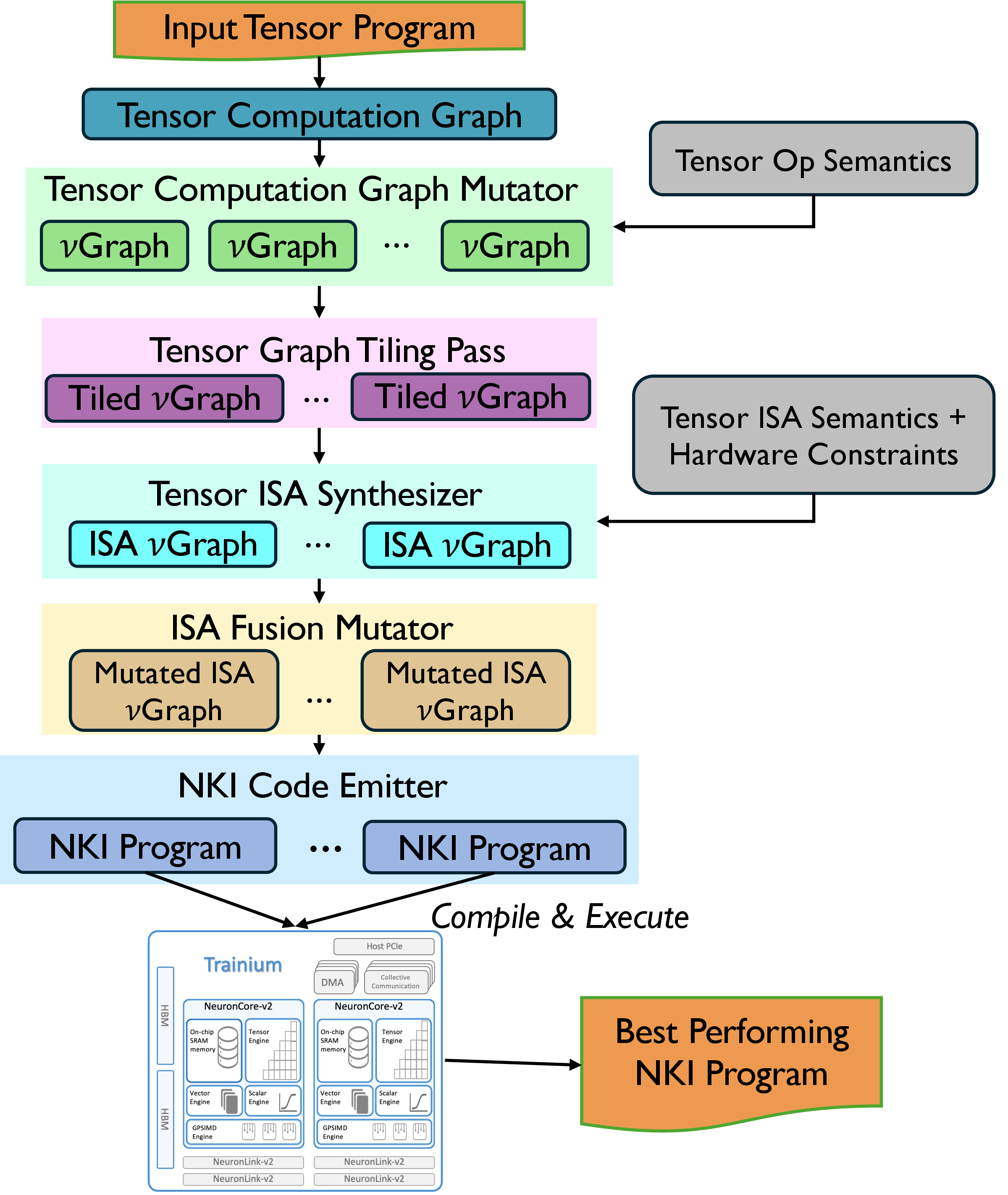
Axon then lowers each tensor operation to target ISA instructions via sketch-driven program synthesis, using semantics specifications that describe each instruction’s computation and hardware constraints. It explores tiling configurations using symbolic parameters constrained by the hardware description, and fuses operators and instructions to minimize memory traffic. All valid variants—across algebraic transformations, instruction selections, tiling configurations, and fusion choices—are maintained simultaneously in a \(\nu\)Graph (“nu-graph”), a persistent internal representation that tracks all semantically equivalent program variants through each stage of the synthesis pipeline. The best-performing kernel is selected empirically when input shapes are known.
Existing approaches to tensor program optimization either require hand-crafted rewrite rules for algebraic transformations [5]–[7], rely on hand-written templates for code generation [8], or target only CPUs and GPUs [9]–[11]. Axon derives all transformations and instruction selections from semantics specifications, enabling it to automatically generate optimized kernels for tile-based AI accelerators with provable correctness guarantees.
Contributions. This paper makes the following contributions:
A provably correct methodology for algebraic transformations through operator propagation, which automatically discovers semantically equivalent computation graphs by decomposing tensor operations into granular computations and using SMT over unbounded tensors. It checks that reordering adjacent operators preserves semantics—requiring no hand-crafted rewrite rules or operator properties.
A synthesis-based pipeline for tile-based AI accelerator programs that automatically lowers high-level tensor operations to target ISA instructions, explores tiling configurations constrained by hardware descriptions, and performs operator and instruction fusion. All semantically equivalent variants are maintained simultaneously and the best-performing kernel is selected empirically.
An evaluation on Amazon’s Trainium across 20 benchmarks spanning individual operators and multi-operator LLM kernels (including Group Query Attention and Gated MLP), demonstrating speedups of up to 3.7x on individual operators and up to 19x on multi-operator kernels over Amazon’s Neuron compiler, up to 1.35x over hand-optimized NKI kernels, and geomean speedups of 2–10% over Mirage [8] on all benchmarks it supports—while synthesizing 16 additional kernels that Mirage cannot.
2 Motivation↩︎
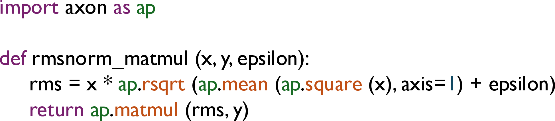
We illustrate Axon’s approach using a kernel composed of RMSNorm [12] followed by a matrix multiplication—a computation pattern that appears multiple times per transformer layer in modern LLMs such as LLaMA-3 [13], where RMSNorm precedes each linear projection (QKV, output, and FFN layers). Figure 2 shows how a programmer expresses this kernel in NumPy-like [4] interface; the rest of this section walks through how Axon automatically optimizes it.
RMSNorm normalizes an input tensor \(X\) by its root mean square (RMS) along a particular dimension (typically the last dimension of \(X\)): \[\text{RMSNorm}(X) = X \odot \text{RMS}(X) = X \odot \frac{1}{\sqrt{\frac{1}{N}\sum_{i} X_i^2 + \epsilon}}\] where \(\epsilon > 0\) is a small constant for numerical stability. The output is then matrix-multiplied with a weight tensor \(W\) to produce the final result \(Z\).
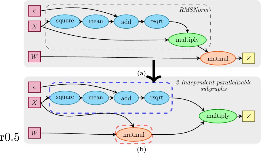
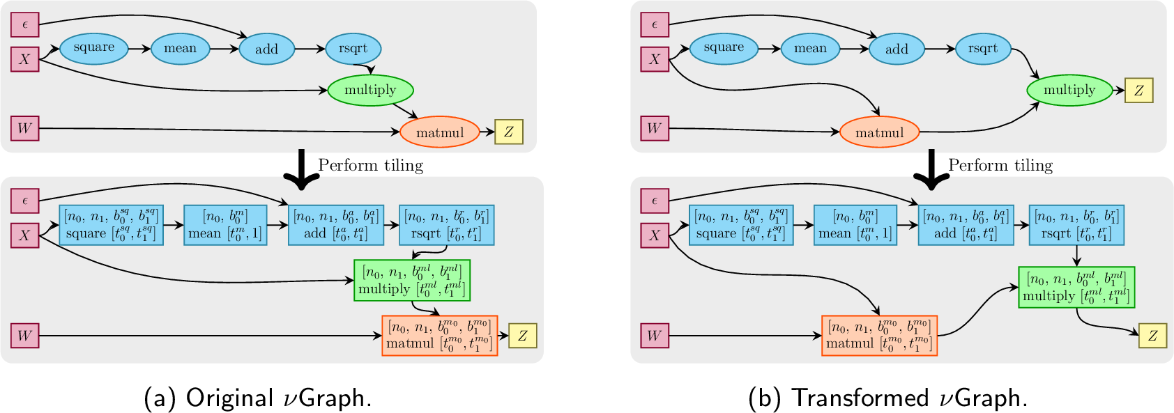
Figure 3 (a) shows the computation graph: the input \(X\) is squared, reduced via mean, passed through rsqrt, multiplied with the original \(X\), and finally given to matmul with weight matrix \(W\).
2.0.0.1 Algebraic Transformations.
On accelerators such as Trainium, executing this graph naively requires all operations to execute sequentially—the normalization must complete before the matrix multiplication can begin, underutilizing the available parallel compute engines.
Axon discovers that the element-wise multiply can be reordered with matmul: instead of computing \((X \odot \text{rms}(X)) \cdot W\), we can compute \((X \cdot W) \odot \text{rms}(X)\). This is valid because \(\text{rms}(X)\) reduces along the last dimension of \(X\)—the same dimension contracted by
matmul—so the element-wise scaling commutes with the matrix multiplication. Axon provably checks semantic equivalence by decomposing both operations into granular computations and using SMT over unbounded tensors
(Section 5), without requiring any hand-crafted rewrite rules.
The transformed graph in Figure 3 (b) exposes two independent subgraphs: matmul executes on the Tensor Engine while the RMS computation executes on the Scalar and Vector Engines in parallel
(Section 3). Rather than committing to a single transformation, Axon maintains both the original and transformed graphs simultaneously in a \(\nu\)Graph
(“nu-graph”)—a persistent internal representation that tracks all semantically equivalent program variants through each stage of the synthesis pipeline (Section 4).
Previous works such as TASO [5], Tensat [6], and Constable [14] use 91 hand-implemented rewrite rules1 to perform graph rewrites. However, none of these works support this transformation. Although this particular rewrite could be added to the existing set of rules, implementing rewrite rules by hand for different combinations of tensor operators is error-prone, as demonstrated by recent efforts to formally verify such rules [15]. Mirage [8] does support this particular rewrite, but fails on a similar transformation in Softmax+MatMul (Appendix 10.1). This is due to a fundamental limitation shared by all graph rewriting systems: they expect operations to appear in specified patterns and do not automatically reason about the semantics of operations to drive algebraic transformations.
2.0.0.2 Tiling.
After discovering algebraic transformations, Axon tiles each tensor operation for the target hardware at multiple levels—from the granular units consumed by individual instructions up to the groups of data that reside in on-chip buffer simultaneously (Section 4.3). The transformed RMSNorm+MatMul graph now has two parallel branches, and Axon introduces independent symbolic tiling parameters for each branch—enabling each to be optimized separately for its respective compute engine and on-chip buffer budget. Different compute engines impose different constraints on tile dimensions, and the optimal grouping of tiles depends on the trade-off between data reuse and on-chip buffer capacity. Axon generates multiple versions with different tiling configurations and selects the best empirically (Section 4.6).
2.0.0.3 ISA Synthesis.
Axon then lowers each tiled 2-D tensor operation to target ISA instructions via program synthesis. For instance, on Trainium, the matmul operation must be lowered to the NKI instruction nc_matmul,
which computes \(\mathbf{a}^\top \mathbf{b}\)—the first operand is consumed in transposed form. The synthesizer discovers that matmul(x, y) can be implemented as nc_matmul(nc_transpose(x), y), and
provably checks this using SMT-based equivalence checking (Section 5). For the element-wise operations in the RMS branch, the synthesizer explores multiple Trainium instruction choices—tensor_tensor,
tensor_scalar, or activation—each with different performance characteristics and tile dimension constraints. All valid instruction selections are maintained simultaneously in the \(\nu\)Graph
(Section 4).
2.0.0.4 Fusion.
After ISA synthesis, Axon identifies opportunities to fuse operations at two levels. Node fusion merges consecutive operations that share compatible tiling dimensions into a single loop nest, so that intermediate
results remain in on-chip buffers rather than spilling to HBM. For example, in the RMS branch, consecutive element-wise operations (such as add_epsilon and rsqrt) can be fused to eliminate an HBM round-trip for the intermediate
tensor. Instruction fusion replaces sequences of ISA instructions with fused variants: for example, on Trainium, a dma_copy followed by nc_transpose can be replaced with the NKI instruction dma_transpose,
performing the layout transformation on-the-fly during data transfer. Additionally, ISA synthesis may introduce new operations (e.g., nc_transpose on Trainium to satisfy nc_matmul’s transposed-input requirement) that create new
fusion opportunities not visible in the original graph.
2.0.0.5 Code Generation and Selection.
Finally, Axon extracts concrete NKI programs from the \(\nu\)Graph by instantiating symbolic tiling parameters with specific values. Each candidate program—encoding a specific combination of algebraic rewrite, instruction selection, tiling configuration, and fusion decisions—is compiled by the Neuron compiler and executed on Trainium. Axon returns the best-performing kernel along with its configuration. The full NKI kernel generated by Axon for this example is shown in Appendix 12.
3 Background↩︎
AI accelerators differ in architectural details, but they share common patterns, e.g., specialized units for computing matmuls, multi-level memory hierarchies, and a reliance on tiling and tuning to achieve peak performance. Tile-based kernel languages exist for various accelerators—NKI for Amazon’s Trainium [1], Pallas for Google’s TPU [2], and cuTile [16] or Triton [3] for GPUs—that expose architectural features through Python-based interfaces. This section introduces these concepts using Amazon’s first-generation Trainium as a concrete example.
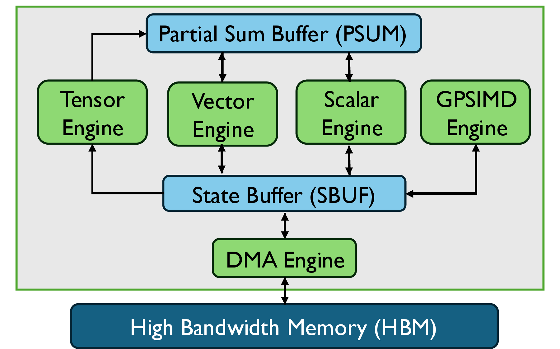
Figure 4: Trainium’s NeuronCore [17]..
3.1 Trainium Architecture↩︎
Figure 4 illustrates the architecture of a NeuronCore, the fundamental compute unit in Trainium. Each Trainium chip contains two NeuronCores. A NeuronCore comprises four specialized compute engines: (1) a Tensor Engine (systolic array) for matrix multiplications, (2) a Vector Engine for vector operations, (3) a Scalar Engine for scalar operations, and (4) a Gpsimd Engine, a general-purpose SIMD unit. All four engines can execute in parallel.
A NeuronCore has High Bandwidth Memory (HBM) and on-chip buffers: State Buffer (SBUF), the primary data buffer accessible by all compute engines, and Partial Sum Buffer (PSUM), an accumulator for the Tensor Engine. DMA engines move data between HBM and SBUF, and can operate in parallel with the compute engines.
3.2 Tile-Based Programming in NKI↩︎
In tile-based programming, computation is structured around fixed-size sub-arrays called tiles that are explicitly moved between HBM and on-chip SRAM buffers, with operations expressed at the tile granularity [3], [18]. Neuron Kernel Interface (NKI) [1] is a Python-based tile-based language for implementing custom kernels on Trainium. NKI kernels follow three stages: (1) loading tiles from HBM to SBUF via DMA, (2) performing on-chip computations on tiles, and (3) writing result tiles back from SBUF to HBM.
Figure 5 shows a tiled matrix multiplication kernel in NKI, adapted from the NKI tutorial [19].
NKI kernels are Python functions decorated with @nki.jit (line 1). The left-hand operand is provided pre-transposed (lhsT) because nc_matmul consumes its stationary operand in transposed form. The kernel iterates over
output tiles (lines 11–12) and the reduction dimension (line 15), loading input tiles from HBM to SBUF via dma_copy (lines 17–20), performing the matrix multiplication on the Tensor Engine via nc_matmul which accumulates results
into PSUM (line 23), and storing the result back to HBM via SBUF (lines 26–28).
Each compute engine enforces hardware constraints on tile dimensions: on Trainium, the partition dimension is at most 128 elements (T_K, T_M), while the free dimension of the moving operand can be up to 512 (T_N)
(lines 5–7). Effective tiling maximizes on-chip data reuse and minimizes DMA traffic between HBM and SBUF.
None
Figure 5: NKI kernel for tiled matrix multiplication on Trainium. The code iterates over tiles (lines 11–12), loads tiles from HBM to SBUF (lines 17–20), computes on-chip via nc_matmul (line 23), and stores results back to HBM
(lines 26–28). Tile dimensions (TILE_K=128, TILE_N=512) are constrained by the hardware..
3.3 Beyond Trainium↩︎
Adapting Axon to target a new platform that implements a similar architecture would require providing new ISA semantics and hardware constraints, and modifying the code emitter to generate kernels for the new target; the core algorithms—algebraic transformations, tiling exploration, synthesis, and fusion—would remain unchanged. However, not all accelerator programming models are a good fit for Axon’s current design. Many-core accelerators such as Meta’s MTIA [20] and Microsoft’s Maia [21] follow fundamentally different execution models without the specialized multi-engine architecture that Axon relies on. GPU kernel languages such as Triton [3], while tile-based, expose a thread-block execution model with shared memory and warp-level primitives that differ substantially from the DMA-driven, engine-parallel model of accelerators like Trainium. Extending Axon to these platforms would require rethinking the ISA synthesis and fusion strategies to account for their distinct execution models.
4 Design↩︎
This section describes the technical details of each stage in Axon’s synthesis pipeline. We first introduce the \(\nu\)Graph (Section 4.1), the persistent internal representation that tracks all semantically equivalent program variants throughout the pipeline. We then describe each pipeline stage: algebraic transformations via operator propagation (Section 4.2), symbolic tiling (Section 4.3), ISA instruction synthesis (Section 4.4), operator and instruction fusion (Section 4.5), and code emission with empirical selection (Section 4.6). We continue to use the RMSNorm+MatMul kernel introduced in Section 2 as our running example.
4.1 \(\nu\)Graph↩︎
A key challenge in superoptimization is maintaining multiple semantically equivalent program variants simultaneously—across algebraic reorderings, tiling configurations, instruction selections, and fusion choices—without committing to any single choice prematurely. Equality saturation [22] addresses a similar problem using e-graphs, which compactly represent a set of semantically equivalent program terms by grouping equivalent sub-expressions into e-classes [14]. Axon extends this idea to dataflow graphs of tensor operations with a structure we call a \(\nu\)Graph.
Definition 1 (\(\nu\)Graph). A \(\nu\)Graph \(\mathcal{G} = (\mathcal{V}, M)\) consists of:
\(\mathcal{V} = \{G_0, G_1, \ldots, G_n\}\): a set of semantically equivalent dataflow graph variants, where each \(G_i\) is a directed acyclic graph of tensor operations;
\(M\): metadata associated with each operation, which accumulates as the \(\nu\)Graph is lowered through the synthesis pipeline.
Unlike standard e-graphs, which track equivalence classes of sub-expressions within a single program, a \(\nu\)Graph tracks equivalence classes of entire dataflow graphs. Each variant carries its own copy of metadata \(M\): when a new variant is created (e.g., by an algebraic transformation or an ISA synthesis choice), it receives a fresh copy of the metadata with its own constraints. The metadata \(M\) evolves through the pipeline stages:
After algebraic transformations (Section 4.2): multiple graph variants \(\{G_0, \ldots, G_n\}\) representing different operator orderings.
After tiling (Section 4.3): symbolic tiling parameters—strip dimensions \([n_0, n_1]\), block dimensions \([b_0, b_1]\), and tile dimensions \([t_0, t_1]\)—for each operation.
After ISA synthesis (Section 4.4): target ISA instructions, hardware constraints on tile dimensions, and compute engine assignments.
4.1.0.1 Exploration and extraction.
Like equality saturation, the \(\nu\)Graph follows an exploration phase and an extraction phase. During exploration, each pipeline stage may expand the set of variants: algebraic transformations generate alternative operator orderings, tiling introduces multiple block size configurations, and ISA synthesis discovers different instruction sequences for the same operation. These choices compose multiplicatively—for example, 2 algebraic variants \(\times\) 4 tiling configurations \(\times\) 3 instruction choices yields 24 candidate programs. During extraction (Section 4.6), Axon instantiates the symbolic parameters, emits concrete programs from the \(\nu\)Graph, and selects the best-performing one through empirical evaluation on the target hardware.
4.1.0.2 Example.
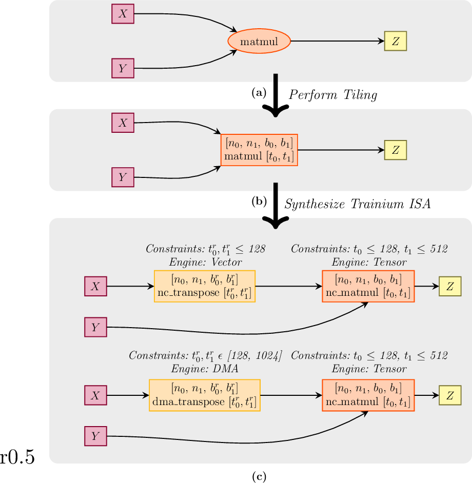
Figure 6 illustrates the \(\nu\)Graph progression on a matmul example. In (a), the \(\nu\)Graph is a high-level dataflow graph with a single
matmul operation. In (b), after tiling, the operation is annotated with symbolic tiling parameters: \([n_0, n_1]\) for strip, \([b_0, b_1]\) for block dimensions, and \([t_0, t_1]\) for tile dimensions. Note that this tiling strategy reflects the two-level memory hierarchy of AI accelerators such as Trainium (HBM and on-chip SRAM), where computations and data movement occur at tile
granularity. In (c), after ISA synthesis, the single matmul has been lowered to two variant instruction sequences—one using nc_transpose on the Vector Engine (with tile constraints \(t_0^r, t_1^r \leq
128\)) and another using dma_transpose on the DMA Engine (with tile constraints \(t_0^r, t_1^r \in [128, 1024]\))—both followed by nc_matmul on the Tensor Engine. Both variants coexist in
the \(\nu\)Graph with their respective hardware constraints; the best is selected empirically after code emission.
4.1.0.3 Benefits and limitations.
By deferring all optimization choices to empirical selection, the \(\nu\)Graph avoids heuristic-based decisions that may be suboptimal for specific input shapes or hardware configurations. It enables joint exploration across all optimization dimensions rather than making greedy sequential decisions that foreclose later opportunities. However, because the number of variants grows multiplicatively across pipeline stages, Axon enumerates all valid combinations and relies on the target backend to reject infeasible ones (e.g., programs that exceed on-chip buffer capacity). In practice, this approach is tractable for kernel-sized programs: ML kernels typically contain fewer than 10 operators per layer, and the resulting search space (up to \({\sim}\)30K candidates for complex kernels such as GQA and Gated MLP) can be evaluated within two hours as a one-time cost (Section 6.5).
4.2 Tensor Computation Graph Mutator↩︎
The Tensor Computation Graph Mutator takes a tensor computation graph as input and performs provably correct, graph-level algebraic transformations to enable better parallelization, ISA fusion, and loop fusion opportunities. As illustrated in
Section 2, the key insight is that certain operations can be reordered while preserving semantic equivalence—for example, propagating the multiply operation past matmul in the
RMSNorm+MatMul kernel enables parallel execution of independent subgraphs. Since multiple valid transformations may exist, each exposing different optimization opportunities, Axon maintains all discovered variants of
semantically equivalent \(\nu\)Graphs \(\{G_0, G_1, \ldots, G_n\}\).
Definition 2 (Semantic Equivalence). Two computation graphs \(G_1\) and \(G_2\) are semantically equivalent, denoted \(G_1 \equiv G_2\), if for all input tensors satisfying the operator preconditions (Section 4.2.1), both graphs produce identical output tensors.
Axon preserves all variants where \(G_0 \equiv G_1 \equiv \cdots \equiv G_n\) and selects the best-performing one empirically when concrete input shapes are known (Section 4.6). Although the number of variants is worst-case exponential, in practice most operator pairs are not swappable and ML kernels typically contain < 10 operators.
4.2.0.1 Operator Propagation.
To discover algebraic transformations, Axon uses a worklist-based algorithm that attempts to propagate each operation downward through the computation graph by swapping it with its successors. For each operator, the algorithm repeatedly checks whether swapping it with an adjacent successor preserves semantic equivalence (Section 5); if so, the new graph variant is added to the \(\nu\)Graph and propagation continues from the new position. The process saturates when no further swaps are possible for any operator, ensuring that all reachable reorderings are explored. Note that by pushing operators down, other operators are inevitably moved up; therefore, upward propagation is unnecessary. Algorithm 9 formalizes this process.

Algorithm 9 generates the \(\nu\)Graph variants as follows. Starting with the original computation graph \(G_0\) (line 1), the algorithm iterates over each operator \(op_1\) in topological order and attempts to propagate it downward (line 2). For each existing graph variant, it initializes a worklist with the current position of \(op_1\) (line 5). The algorithm repeatedly pops a (graph, position) pair from the worklist (line 7) and examines each immediate successor \(op_2\) (line 8). For each successor, it retrieves the input operands \(\mathcal{I}\) of \(op_1\) (line 9) and attempts swaps with progressively increasing clone degree \(k\) (lines 10–11): \(k\) determines how many of \(op_1\)’s inputs pass through \(op_2\) in the swap, preferring the smallest \(k\) that yields a valid transformation (lines 17–18). For each subset \(S \subseteq \mathcal{I}\) of size \(k\), \(\textsf{SwapWithSuccessor}\) constructs the swapped graph, and \(\textsf{CheckEquivalence}\) provably checks whether the swap preserves semantic equivalence (Section 5). The algorithm prefers the smallest clone degree that yields a valid swap (lines 17–18). If the check passes, the new variant is saved and pushed onto the worklist to continue propagating (lines 13–15); if no swap is possible, the current graph is retained (lines 19–20). After processing all operators, the algorithm returns the complete set of semantically equivalent graph variants.
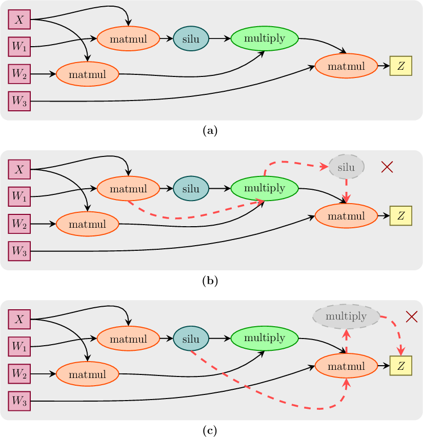
For example, in Figure 3, the algorithm discovers that multiply can be propagated past matmul, producing the transformed graph in (b). In contrast, Figure 7 shows the Gated MLP kernel where propagation attempts fail the equivalence check, so no new variants are generated.
4.2.1 Semantics of Tensor Operations↩︎
Programmers provide operational semantics for the high-level tensor operations they use in their programs, as shown in Figure 10 for the matmul operation. The semantics specification includes three key
components:
Rank and shape preconditions: Requirements on tensor ranks and dimension compatibility for a given tensor operation. In the example,
a.min_rank() == 2requires that the input tensors have at least two dimensions, anda.shape[-1] == b.shape[-2]ensures the contraction dimensions of the input tensors match.Access maps: How input tensors are indexed, defined via symbolic axes (akin to affine maps in MLIR [23]). The expression
a[..., i0, i1]uses NumPy-like indexing style to denote accessing an element at given indices.Granular semantics: The element-level operations expressed using granular operators. The expression
mul(a[..., i0, i1], b[..., i1, i2]).sum(axis=i1)specifies multiply-accumulate over the contraction axisi1. These expressions are converted to SMT formulas used for equivalence checking (Section 5).
This allows programmers to define custom high-level, hardware-agnostic tensor operations.
4.3 Tensor Graph Tiling Pass↩︎
The Tiling Pass prepares the Tensor Computation \(\nu\)Graph for ISA synthesis by introducing symbolic tiling parameters. This transformation tiles each operation with symbolic strip, block, and tile dimension sizes, and converts N-D tensor operations into 2-D operations enclosed in loops. Loops are not explicitly represented; instead, we use a compact representation showing symbolic dimensions.
4.3.0.1 Tiling Notation.
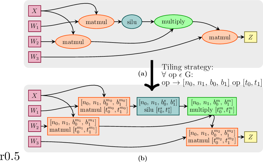
Figure 8 illustrates the tiling notation using the Gated MLP example, where \(x\) is the input tensor and \(w_1\), \(w_2\), \(w_3\) are weight matrices. Each operation is annotated with \([n_0, n_1, b_0, b_1]\;op\;[t_0, t_1]\), where:
\([t_0, t_1]\): Tile dimensions—the size of each 2-D tile processed by a single instruction for a compute engine. These are determined by hardware constraints of the target instructions (described in Section 4.4).
\([b_0, b_1]\): Block dimensions—the number of tiles grouped into a block along each dimension. Blocking enables data reuse by keeping data in on-chip SRAM (SBUF/PSUM) across multiple tile operations; larger blocks increase reuse but are constrained by the capacity of on-chip SRAM. Block dimension size selection also impacts DMA utilization, as the DMA engine can move multiple tiles between HBM and SBUF; therefore, small block sizes can lead to DMA bandwidth underutilization.
\([n_0, n_1]\): Strip dimensions—the number of blocks along each dimension in HBM, computed as \(\bigl[\ceil{\tfrac{M}{b_0 t_0}},\;\ceil{\tfrac{N}{b_1 t_1}}\bigr]\) for a tensor of shape \([M, N]\).
None
Figure 10: Semantics of matmul tensor operation in Axon..
For example, in Figure 8, the first matmul operation (\(X \cdot W_1\)) has block dimensions \([b_0^{m0}, b_1^{m0}]\) and tile dimensions
\([t_0^{m0}, t_1^{m0}]\), where the superscript \(m0\) identifies these as the first matmul’s parameters. Similarly, the silu operation has its own parameters \([b_0^{s}, b_1^{s}]\) and \([t_0^{s}, t_1^{s}]\), and subsequent matmuls use superscripts \(m1\), \(m2\). Since the optimal block
size depends on the trade-off between data reuse and on-chip buffer capacity, Axon uses symbolic parameters and generates multiple versions with block sizes ranging from 1 to 32 tiles (bounded by SBUF capacity on Trainium),
selecting the best-performing configuration empirically (Section 4.6). Strip dimensions along which no reduction occurs are shared across all tensor operators in a computation graph (\([n_0, n_1]\)) to maximize data reuse of on-chip blocks across operators and facilitate fusion opportunities later in the synthesis pipeline.
4.3.0.2 Tiling and Operator Reordering.
Figure 11 shows how tiling interacts with the algebraic transformations from Section 4.2. In the original graph (a), operations execute sequentially:
square, mean, rsqrt, multiply, then matmul. Each operation has its own tiling parameters (e.g., \([n_0, n_1, b_0^{sq}, b_1^{sq}]\) for square).
In the transformed graph (b), propagating multiply past matmul creates two parallel branches: the RMS computation (blue) and the matrix multiplication (red). Because these branches execute on different compute engines with
different hardware constraints—the Tensor Engine for matmul and the Vector/Scalar Engine for RMS—they can have independent tiling parameters, enabling each branch to be optimized separately for its respective engine and on-chip memory budget.
@p5.8cmp8cml@ API & Description & Engine
_copy(dst, src) & Copy data between HBM and SBUF & DMA
_copy(src, engine) & Create a copy of tile within on-chip SRAMs (SBUF/PSUM) & Scalar/Vector/Gpsimd
_transpose(src, axes) & Transpose tile via DMA (supports 2D/3D/4D) & DMA
_transpose(data, engine) & 2D transpose between partition and free axes of tile & Vector/Tensor
_matmul(stationary, moving) & Matrix multiplication: \(\mathbf{stationary}^\top \mathbf{moving}\) & Tensor
(op, data, bias, scale) & Apply activation function with optional scale/bias & Scalar
(data) & Elementwise reciprocal of tile (\(1.0/x\)) & Vector
_tensor(data1, data2, op, engine) & Elementwise binary operation between two tiles & Vector/Gpsimd
& & Vector/Scalar/Gpsimd
& & Vector
_reduce(op, data, axis) & Reduction along free axes of tile & Vector
_partition_reduce(op, data) & Reduction across partitions of tile & Gpsimd
& & Vector
& & Vector
4.4 Tensor ISA Synthesizer↩︎
The Tensor ISA Synthesizer lowers each 2-D tensor operation in the Tiled \(\nu\)Graph to equivalent sequences of target ISA instructions using program synthesis.
4.4.0.1 ISA Semantics.
Axon uses two levels of semantics specifications. Tensor operator semantics (Section 4.2.1, Figure 10) describe high-level operations
such as matmul and reduce_sum, and are provided by programmers writing tensor programs. ISA instruction semantics describe hardware-specific instructions such as Trainium’s nc_matmul and
nc_transpose, and are provided once per target by compiler developers with knowledge of the hardware. Both use the same @semantics interface (preconditions, access maps, granular semantics), but ISA semantics additionally include
hardware constraints that specify valid tile dimension ranges for each instruction. This separation means tensor operator semantics can be shared across targets, while ISA semantics are specified per target architecture.
Figure 12 shows the ISA semantics for Trainium’s nc_matmul, which computes \(\mathbf{a}^\top \mathbf{b}\). The hardware constraints (K <= 128,
M <= 128, N <= 512) reflect the Tensor Engine’s tile dimension limits on Trainium. These constraints are imposed on the symbolic tiling parameters from Section 4.3, ensuring that
synthesized code respects hardware limitations when emitting code in Section 4.6.
None
Figure 12: ISA semantics of Trainium’s nc_matmul instruction. Unlike the tensor operator semantics for matmul (Figure 10), this specification includes hardware constraints and reflects
the transposed access pattern (a[i1, i0])..
4.4.0.2 Synthesis Algorithm.
Axon uses a two-phase sketch-driven synthesis approach (Algorithm 13). In Phase 1, Axon builds an instruction pool \(\mathcal{P}\) by filtering ISA instructions to those sharing constituent operations with the tensor operation \(T\) being lowered (lines 1–8). For example, if \(T\)’s granular semantics (Section 4.2.1) include add and multiply operations, only ISA instructions that perform at least one of these operations are
added to \(\mathcal{P}\), reducing the search space. Instructions performing data layout transformations such as transpose are also included. The algorithm first retrieves the input operands \(\mathcal{I}\) of \(T\) (line 1)—for example, \(\mathcal{I} = \{x, y\}\) for \(\texttt{matmul}(x, y)\). For each ISA instruction
added to \(\mathcal{P}\), Axon generates variants with its operand slots filled by either inputs from \(\mathcal{I}\) or holes (\(\square\)) to be resolved during composition in Phase 2 (lines 4–8). In Phase 2, Axon recursively fills holes in sketches with instructions from the pool (lines 9–19): starting from a sketch with
a single hole, it pops candidates from a worklist, fills each hole with instructions from \(\mathcal{P}\), and checks complete candidates for provable equivalence with \(T\) using \(\textsf{CheckEquivalence}\) (Section 5).
For example, when lowering MatMul(x, y), the synthesizer explores compositions such as: \[\operatorname{MatMul}(x, y)
\overset{?}{=}
\operatorname{nc\_matmul}\!\big(\operatorname{nc\_transpose}(x),\; y\big)\] Since nc_matmul(a,b) computes \(\mathbf{a}^\top \mathbf{b}\), the transpose is required to match standard matrix multiplication
semantics. On Trainium, an instruction depth limit of 3 is sufficient to synthesize all supported tensor operations, because the ISA is coarse-grained: each high-level tensor operation lowers to at most 3 ISA instructions.
4.4.0.3 Synthesis Example.
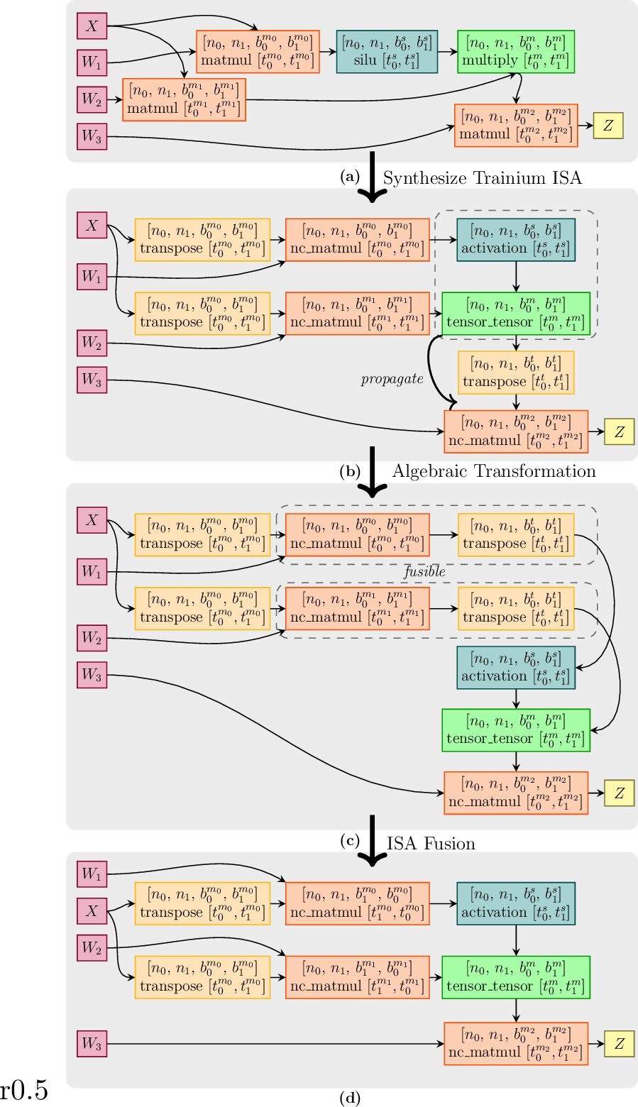
Figure 14 illustrates the synthesis process on the Gated MLP kernel. In part (a), the tiled \(\nu\)Graph contains high-level operations like matmul, silu, and
multiply. Part (b) shows the ISA \(\nu\)Graph after synthesis: notably, each matmul is lowered to transpose followed by nc_matmul, because nc_matmul expects
its first operand to be transposed (as specified in the ISA semantics of Figure 12). The annotations show valid tile dimension ranges extracted from hardware constraints (e.g., [1-128, 1-128] for
nc_matmul).
4.4.0.4 DMA Operations and Engine Selection.
After synthesizing compute instructions, Axon generates DMA copy instructions to transfer data between HBM and on-chip SRAM. Additionally, since Trainium allows users to select which compute engine executes each instruction, Axon represents all valid engine variants in the \(\nu\)Graph, deferring the final selection to empirical evaluation.
4.5 ISA Fusion Mutator↩︎
The ISA Fusion Mutator performs a second round of algebraic transformations (as described in Section 4.2), but this time at the ISA instruction level to expose ISA and operator (loop nest) fusion. This second round is necessary because ISA synthesis (Section 4.4) may introduce new operations that were not present in the original computation graph, and the new operations create transformation opportunities that the Graph Mutator (Section 4.2) could not have discovered.
For example, in the Gated MLP kernel (Figure 14 (a)), lowering matmul introduces a transpose operation since it is required by nc_matmul’s semantics (Figure 14 (b)). Axon explores valid algebraic transformations on the newly generated ISA \(\nu\)Graph. It discovers that the last transpose operation can be
moved past the activation and tensor_tensor instructions (Figure 14 (c)), since both are element-wise instructions that commute with transpose. Once there are no further algebraic
transformations that yield new variants, Axon looks for fusion opportunities on adjacent nodes of the \(\nu\)Graph. It identifies two fusion opportunities: the two nc_matmul
operations and their succeeding transpose operations are fusible, producing the graph in Figure 14 (d).
The mutator performs two types of fusion:
4.5.0.1 Instruction Fusion.
The mutator performs peephole optimizations by replacing two or more instructions in ISA \(\nu\)Graphs with a single, semantically-equivalent instruction. This is achieved using the same synthesis algorithm as Section 4.4 (Algorithm 13), but with depth 1 since the goal is to fuse two instructions into one. In Figure 14, nc_matmul and the succeeding
transpose operations are fused into a new nc_matmul but with swapped operands—Axon discovers via synthesis that \(\operatorname{transpose} (\operatorname{nc\_matmul}(X.t,
W)) \rightarrow \operatorname{nc\_matmul}(W, X.t)\). This effectively eliminates an intermediate data layout transformation. Superoptimizers such as Mirage [8] do not support such a rewrite.
Other examples include fusing activation and tensor_reduce to activation_reduce, and tensor_scalar and tensor_reduce to tensor_scalar_reduce. This pass also fuses
dma_copy with dma_transpose to allow on-the-fly transpose when reading from or writing to HBM.
4.5.0.2 Operator/Loop Fusion.
This is more similar to the traditional fusion optimization: consecutive nodes of the \(\nu\)Graphs with the same strip dimensions, across which no reduction occurs, are deemed fusible along those dimensions. (Reductions
such as mean in RMSNorm [12] require processing an entire tensor row before normalization, preventing fusion across that dimension.) This
improves data locality and decreases memory traffic between HBM and SBUF. Axon also fuses nodes of independent subgraphs to enable deep fusion of loop nests, leveraging compute and data movement parallelism across different
engines.
4.6 NKI Code Emitter↩︎
The NKI Code Emitter is the final stage of Axon’s synthesis pipeline. It traverses the mutated ISA \(\nu\)Graph to extract concrete NKI programs, where each program represents a specific combination of algebraic rewrite, instruction selection, tiling configuration, and fusion decisions. The symbolic block sizes from Section 4.3 are instantiated with concrete values, generating multiple candidates per \(\nu\)Graph.
Each emitted NKI program is then passed to the Neuron compiler [24], which handles on-chip buffer allocation (assigning SBUF and PSUM addresses to intermediate tensors) and produces the final executable. Because Axon does not directly control on-chip SRAM allocation, some candidates that satisfy Axon’s symbolic tile constraints may still be rejected by the Neuron compiler—for example, when the cumulative size of live tiles in a block exceeds the physical SBUF capacity. This is why not all emitted programs are compilable (Section 6.5).
Empirical execution and random testing. For the candidates that are successfully compiled to binaries by the Neuron compiler, Axon executes them on the target hardware, measures latency, and validates numerical correctness against a reference implementation on random inputs. We deem the outputs numerically equivalent if they satisfy, elementwise, \(\lvert \mathrm{emitted\_code}-\mathrm{reference}\rvert \le \texttt{atol}+\texttt{rtol}\,\lvert \mathrm{reference}\rvert\) with \(\texttt{rtol}=10^{-4}\) (relative error) and \(\texttt{atol}=10^{-4}\) (absolute error) on FP32 data type. Axon then returns the best-performing NKI program along with its configuration (tile sizes, instruction choices, fusion decisions). This empirical selection ensures that the final kernel is optimized for the specific input shapes and target hardware.
5 Correctness of Transformations↩︎
Every transformation that Axon performs—whether reordering operators in the computation graph (Section 4.2), synthesizing ISA instruction sequences (Section 4.4) or fusing instructions (Section 4.5)—must preserve semantic equivalence. This section describes how Axon leverages SMT-based reasoning to provably check that each transformation is correct.
5.1 Equivalence Checking Methodology↩︎
Axon’s equivalence checking adapts the methodology introduced by TensorRight [15]—originally designed to verify XLA rewrite rules—to provably check transformations from operator propagation (Section 4.2) and ISA synthesis (Section 4.4).
5.1.0.1 Encoding.
To provably check that two tensor expressions are equivalent, Axon encodes each operation’s computation as SMT constraints and checks two conditions:
Shape Condition: The symbolic shapes of output tensors on both sides must be equivalent.
Computation Condition: The computation performed on each element must be equivalent.
Tensors are encoded as uninterpreted functions mapping indices to values (e.g., a rank-2 tensor \(X\) becomes \(X: \mathbb{Z} \times \mathbb{Z} \to \mathbb{R}\)), and dimension sizes are symbolic integers. This allows reasoning over tensors of arbitrary size with known rank—the proof holds for any concrete dimension sizes. Table 1 summarizes how different categories of operations are encoded.
| Category | Operations | SMT Encoding | Axioms |
|---|---|---|---|
| Element-wise | mul, div, add, sub | \(\forall i,j{:}\; out(i,j) = a(i,j) \circ b(i,j)\) | None |
| Unary pointwise | sqrt, relu | \(\forall i,j{:}\; out(i,j) = f(a(i,j))\) | None |
| Reduction | reduce_sum | \(P(i,0){=}0;\;\; P(i,k{+}1){=}P(i,k){+}a(i,k);\;\; out(i){=}P(i,N)\) | Arithmetic axioms |
| Matmul | matmul | \(P(i,j,0){=}0;\;\; P(i,j,k{+}1){=}P(i,j,k){+}a(i,k){\cdot}b(k,j);\;\; out(i,j){=}P(i,j,K)\) | Arithmetic axioms |
| Nonlinear | exp, sigmoid | Uninterpreted function (minimal properties) | Conservative rejection |
| Layout | transpose | \(\forall i,j{:}\; out(i,j) = a(j,i)\) | None |
Table 2 shows the granular operations for key tensor operations and NKI ISA instructions used in the equivalence checking.
For element-wise and layout operations, the encoding is straightforward and the solver can determine equivalence directly. For reductions and matrix multiplications, which involve summation over a contraction dimension, the methodology provides
arithmetic axioms—such as the distributivity of multiplication over summation (\(\operatorname{mul}(\sum f(x),\,v) = \sum \operatorname{mul}(f(x),\,v)\) when \(v\) is invariant over the
summation)—that enable the solver to reason about equivalence of reduction expressions. Nonlinear functions (e.g., exp, sigmoid) are treated as uninterpreted functions: the solver knows only minimal properties (e.g., \(\exp(x) > 0\)) and cannot reason about their algebraic behavior, so swaps involving them are conservatively rejected.
5.1.0.2 Checking procedure.
Given two adjacent operators \(op_1\) and \(op_2\) in the computation graph, Axon checks whether they can be swapped:
Construct the swapped graph by exchanging \(op_1\) and \(op_2\).
Encode both the original and swapped graphs as SMT constraints using the encodings in Table 1.
Check the Shape Condition: prove that output shapes are equal under all valid input shapes.
Check the Computation Condition: prove that for all valid indices, the output values are equal—i.e., \(\forall \vec{i}{:}\; out_{\text{orig}}(\vec{i}) = out_{\text{swap}}(\vec{i})\).
If the solver proves both conditions, the swap is accepted. If the solver returns
unknown(e.g., timeout), the swap is conservatively rejected.
Definition 3 (Swappable successive tensor operations). Let \(OP_1\) and \(OP_2\) be two successive operations in a computation graph \(G\). \(OP_1\) and \(OP_2\) are deemed swappable* if the solver proves that applying \(OP_1\) then \(OP_2\) produces the same output as applying \(OP_2\) then \(OP_1\): \[\llbracket OP_2 \rrbracket\bigl(\llbracket OP_1 \rrbracket(\vec{x})\bigr) \;\;\equiv\;\; \llbracket OP_1 \rrbracket\bigl(\llbracket OP_2 \rrbracket(\vec{x})\bigr)\] where \(\llbracket \cdot \rrbracket\) denotes the semantics of an operation and \(\vec{x}\) represents the input tensors.*
| Operator | Granular Operation |
|---|---|
| matmul(x, y) | \(sum(mul(x_{i,k}, y_{k,j}), dim=k)\) |
| transpose(x) | \(x_{i,k} \to x_{k,i}\) |
| relu(x) | \(max(0, x_{i,j})\) |
| silu(x) | \(mul(x_{i,j}, sigmoid(x_{i,j}))\) |
| nc_matmul(x, y) | \(sum(mul(x_{k,i}, y_{k,j}), dim=k)\) |
| nc_transpose(x, engine) | \(x_{i,k} \to x_{k,i}\) |
| tensor_tensor(x1, x2, op, engine) | \(op(x_{i,j}, y_{i,j})\) |
| tensor_reduce(op, x, axis) | \(op(x_{i,j, red\_dim=j})\) |
| tensor_partition_reduce(op, x) | \(op(x_{i,j, red\_dim=i})\) |
| activation(op, x) | \(op(x_{i,j})\) |
| tensor_scalar(x, op1, y, op2, z, engine) | \(op2(op1(x_{i,j}, y_{i,j}), z_{i,j})\) |
| scalar_tensor_tensor(x, op1, y, op2, z) | \(op2(op1(x_{i,j}, y_{i,j}), z_{i,j})\) |
| tensor_scalar_reduce(x, op1, y, op2, z) | \(op2(op1(x_{i,j}, y_{i,j}), z_{i,j})\) |
r0.55
5.1.0.3 Examples.
Legal swap: multiply past matmul. In the RMSNorm+MatMul kernel (Section 2), Axon checks whether \(\operatorname{MatMul}(\operatorname{Multiply}(X, rsqrt), W) \overset{?}{=} \\ \operatorname{Multiply}(\operatorname{MatMul}(X, W), rsqrt)\). For the Shape Condition: both sides produce shape \([M, N]\) when \(X\) is \([M, K]\), \(rsqrt\) is \([M, 1]\), and \(W\) is \([K, N]\). For the Computation Condition: the LHS computes \(\sum_k (X_{i,k} \cdot rsqrt_i) \cdot W_{k,j}\) and the RHS computes \((\sum_k X_{i,k} \cdot W_{k,j}) \cdot rsqrt_i\). Since \(rsqrt_i\) is invariant over \(k\), the distributivity axiom enables the solver to confirm equivalence. The swap is accepted.
Illegal swap: silu past multiply. In the Gated MLP kernel (Section 4.2), Axon checks whether \(\operatorname{Multiply}(\operatorname{Silu}(X), G) \overset{?}{=} \operatorname{Silu}(\operatorname{Multiply}(X, G))\). The Shape Condition is satisfied (both element-wise, same output shape). For the Computation Condition: the LHS computes \(X_{i,j} \cdot \sigma(X_{i,j}) \cdot G_{i,j}\) and the RHS computes \(X_{i,j} \cdot G_{i,j} \cdot \sigma(X_{i,j} \cdot G_{i,j})\), where \(\sigma\) is the sigmoid function. Since \(\sigma\) is an uninterpreted function, the solver cannot prove these are equal. The swap is rejected.
ISA synthesis: matmul via nc_matmul. During ISA synthesis (Section 4.4), Axon checks whether \(\operatorname{MatMul}(x, y) \overset{?}{=} \operatorname{nc\_matmul}(\operatorname{nc\_transpose}(x), y)\). Since \(\operatorname{nc\_matmul}(a, b)\) computes \(a^T \cdot b\) (Table 2), transposing \(x\) first recovers standard multiplication. The solver confirms both conditions, accepting the synthesized instruction sequence.
5.2 Guarantees and Limitations↩︎
Axon’s equivalence checking guarantees semantic equivalence over all valid inputs for tensors of arbitrary size with known rank. The checking is conservative: if the solver cannot prove equivalence, the transformation is rejected, ensuring no incorrect transformations are applied. This provides stronger correctness guarantees than probabilistic equivalence testing (as used by Mirage [8]), which tests on finite inputs and provides statistical but not provable guarantees.
The approach has two limitations. First, the equivalence checking operates over real-valued arithmetic and does not account for floating-point precision—the generated kernels may exhibit small numerical differences due to rounding, which is standard in
tensor program optimization. We use the solver’s real theory because it is significantly faster than its floating-point theory: as an example, swapping multiply and matmul in the RMSNorm+MatMul kernel alone (Figure 3) takes 247.75 s with floating-point theory and 0.15 s with real theory (1650\(\times\) slowdown). Floating-point theory is prohibitively slow for program synthesis and
verification [25]–[29]. Instead, Axon uses the real theory for algebraic transformations and ISA synthesis, and validates numerical equivalence via testing on random floating-point inputs (Section 4.6). Second, nonlinear functions are treated as uninterpreted, which means the solver may conservatively reject valid swaps involving these functions.
Dynamic shapes are naturally supported by the equivalence checking, since it operates on symbolic dimensions over unbounded tensors and the proofs hold for any concrete dimension sizes.
6 Evaluation↩︎
6.1 Implementation and Experimental Setup↩︎
Axon is implemented in approximately 16,500 lines of Python 3.10 [30]. The equivalence checking engine (Section 5) reimplements TensorRight’s [15] methodology in Python, using Z3 4.12.6 [31] as the SMT solver. Axon takes NumPy-like tensor programs as input and emits NKI programs [1]—the tile-level kernel language for Trainium—which are then processed by the Neuron compiler [24].
Benchmarks. Our benchmark suite includes 11 individual operators—MatMul, RMSNorm, Cumsum, Softmax, RoPE, Tensor Multiply, Max Pooling, ReLU, SiLU, SwiGLU, and GLU—and 9 multi-operator kernels: RMSNorm+MatMul, Matmul+Add+RMSNorm, Softmax+MatMul, Transpose+MatMul, QKV Projection, Group Query Attention (GQA), SiLU Gated MLP, SwiGLU Gated MLP, and Matmul+Matmul+SiLU+Mul. These cover the core computational kernels in modern LLM architectures such as LLaMA-3 [13] and Falcon [32], and significantly overlap with the benchmarks evaluated in Mirage [8]. For each benchmark, we sweep across a range of tensor dimension sizes; since performance depends only on tensor shapes, we repeat each experiment 100 times (and 20 times for warmup) using random inputs and report the average run time.
Baselines. We compare Axon against the following baselines:
Amazon’s Neuron compiler. The Neuron compiler [24] (version
2.21.18209.0+043b1bf7) is the proprietary commercial compiler for Trainium that performs graph-level optimizations and uses hand-tuned heuristics for code generation. As the primary production compiler for Trainium, it serves as a key baseline.Hand-optimized NKI kernels. Amazon provides hand-optimized NKI kernels in the
nki-samplesrepository [33]. Note that hand-optimized NKI kernels are available for only a small subset of operators.Search-based compiler. Mirage [8] has been recently extended to target Trainium for a handful of kernels (RMSNorm+MatMul and Partial Gated MLP). The NKI code generation extension2 was obtained by contacting the authors directly. It uses hand-implemented templates for individual operators such as MatMul and element-wise operators, and composes them based on the kernel specification.
All compilation paths to Trainium go through the Neuron compiler, but enter at different levels: Axon takes NumPy-like programs and emits NKI; Mirage takes custom kernel specifications implemented in C++ and also emits
NKI; the Neuron compiler baseline takes tensor programs written using NumPy [4] and handles all transformations and optimizations—tiling,
operator fusion, instruction selection—internally with its own heuristics; and hand-optimized NKI kernels are written directly in NKI. All emitted NKI programs are processed by the same Neuron compiler backend. All baselines use their default
configurations. For the hand-optimized NKI kernels, we use commit 7af4e4d of the nki-samples repository [33] and the NKI language version is 2.21.18209.0.
Hardware Platform. We run all experiments on an Amazon EC2 trn1.32xlarge instance equipped with 16 Trainium chips with 32 Neuron cores and 128 cores of Intel Xeon Platinum 8375C processors (2.90 GHz, 55 MB L3 cache) with
hyperthreading disabled. We perform our experiments on only one Neuron core to evaluate the effectiveness of Axon’s optimization and code generation on a single core.
We structure our evaluation around four questions:
RQ1: How does Axon perform against existing baselines on individual tensor operators? Although these kernels pass through the full Axon pipeline, the performance gains are primarily due to tiling (Section 4.3) and ISA instruction selection (Section 4.4): individual operators have limited opportunities for algebraic transformations or inter-operator fusion.
RQ2: How does Axon perform on multi-operator kernels, where inter-operator algebraic transformations (Section 4.2) and loop fusion across operators (Section 4.5) provide additional optimization opportunities?
RQ3: What is the contribution of each optimization (such as algebraic transformations, fusion)?
RQ4: What is the compilation overhead of Axon, and how does it scale with kernel complexity?
Not all baselines are available for every benchmark: the Neuron compiler does not support kernels with inter-loop dependencies (e.g., Cumsum); Mirage’s NKI extension only supports MatMul, RMSNorm+MatMul, Softmax+MatMul, and Matmul+Matmul+SiLU+Mul; and hand-optimized NKI kernels are only available for Cumsum and RoPE.
| Benchmark | ||||||||||||||||||||||||||||||||||||||||||||||||||||||||||||||||||||||||||||
|---|---|---|---|---|---|---|---|---|---|---|---|---|---|---|---|---|---|---|---|---|---|---|---|---|---|---|---|---|---|---|---|---|---|---|---|---|---|---|---|---|---|---|---|---|---|---|---|---|---|---|---|---|---|---|---|---|---|---|---|---|---|---|---|---|---|---|---|---|---|---|---|---|---|---|---|---|
| vs Neuron Compiler | ||||||||||||||||||||||||||||||||||||||||||||||||||||||||||||||||||||||||||||
| Multiply | ||||||||||||||||||||||||||||||||||||||||||||||||||||||||||||||||||||||||||||
| RMSNorm | ||||||||||||||||||||||||||||||||||||||||||||||||||||||||||||||||||||||||||||
| ReLU | ||||||||||||||||||||||||||||||||||||||||||||||||||||||||||||||||||||||||||||
| SiLU | ||||||||||||||||||||||||||||||||||||||||||||||||||||||||||||||||||||||||||||
| GLU | ||||||||||||||||||||||||||||||||||||||||||||||||||||||||||||||||||||||||||||
| SwiGLU | ||||||||||||||||||||||||||||||||||||||||||||||||||||||||||||||||||||||||||||
| Softmax | ||||||||||||||||||||||||||||||||||||||||||||||||||||||||||||||||||||||||||||
| MaxPool | ||||||||||||||||||||||||||||||||||||||||||||||||||||||||||||||||||||||||||||
| vs Hand-implemented NKI | ||||||||||||||||||||||||||||||||||||||||||||||||||||||||||||||||||||||||||||
| Cumsum | – | – | – | – | – | |||||||||||||||||||||||||||||||||||||||||||||||||||||||||||||||||||||||
| RoPE | – | – | – | – | – | |||||||||||||||||||||||||||||||||||||||||||||||||||||||||||||||||||||||
1.2pt
6.2 RQ1: Individual Operators↩︎
| Benchmark | ||||||||||||||||||||||||||||||||||||||||||||||||||||||||||||||||||||||||||||||||||
|---|---|---|---|---|---|---|---|---|---|---|---|---|---|---|---|---|---|---|---|---|---|---|---|---|---|---|---|---|---|---|---|---|---|---|---|---|---|---|---|---|---|---|---|---|---|---|---|---|---|---|---|---|---|---|---|---|---|---|---|---|---|---|---|---|---|---|---|---|---|---|---|---|---|---|---|---|---|---|---|---|---|---|
| vs Neuron Compiler | ||||||||||||||||||||||||||||||||||||||||||||||||||||||||||||||||||||||||||||||||||
| Transpose+MM | ||||||||||||||||||||||||||||||||||||||||||||||||||||||||||||||||||||||||||||||||||
| RMSNorm+MM | ||||||||||||||||||||||||||||||||||||||||||||||||||||||||||||||||||||||||||||||||||
| MM+Add+RMSNorm | ||||||||||||||||||||||||||||||||||||||||||||||||||||||||||||||||||||||||||||||||||
| Softmax+MM | ||||||||||||||||||||||||||||||||||||||||||||||||||||||||||||||||||||||||||||||||||
| MM+MM+SiLU+Mul | ||||||||||||||||||||||||||||||||||||||||||||||||||||||||||||||||||||||||||||||||||
| QKV Projection | ||||||||||||||||||||||||||||||||||||||||||||||||||||||||||||||||||||||||||||||||||
| GQA | ||||||||||||||||||||||||||||||||||||||||||||||||||||||||||||||||||||||||||||||||||
| SiLU MLP | ||||||||||||||||||||||||||||||||||||||||||||||||||||||||||||||||||||||||||||||||||
| SwiGLU MLP | ||||||||||||||||||||||||||||||||||||||||||||||||||||||||||||||||||||||||||||||||||
| vs Mirage | ||||||||||||||||||||||||||||||||||||||||||||||||||||||||||||||||||||||||||||||||||
| RMSNorm+MM | ||||||||||||||||||||||||||||||||||||||||||||||||||||||||||||||||||||||||||||||||||
| Softmax+MM | ||||||||||||||||||||||||||||||||||||||||||||||||||||||||||||||||||||||||||||||||||
| MM+MM+SiLU+Mul | ||||||||||||||||||||||||||||||||||||||||||||||||||||||||||||||||||||||||||||||||||
1.2pt
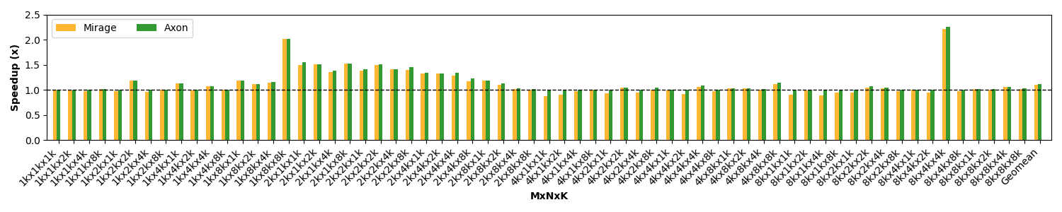
Table 3 and Figure 15 show the performance of Axon on individual tensor operators across a range of tensor dimension sizes.
Against the Neuron Compiler. Across all operators compared against the Neuron compiler—Tensor Multiplication, RMSNorm, Softmax, ReLU, SiLU, GLU, SwiGLU, and Max Pooling (Table 3, top)—Axon matches or slightly outperforms the Neuron compiler at smaller dimension sizes and achieves speedups of up to 3.7x (SiLU at 16384\(\times\)16384) at larger sizes, with geomean speedups ranging from 1.23x (Multiply, MaxPool) to 1.90x (SiLU). The speedups at larger sizes are primarily because the code synthesized by Axon achieves better temporal locality for tiles of data in on-chip buffer and better DMA utilization. The Neuron compiler uses fixed heuristics for tiling that become suboptimal as tensor dimensions grow, whereas Axon systematically explores the space of valid tiling configurations and selects the best-performing one empirically.
Against Mirage. Mirage provides a hand-tuned NKI template only for MatMul among the individual operators. On Matrix Multiplication (Figure 15), Axon achieves performance comparable to Mirage across all dimension sizes, with a geomean speedup of 2% and a maximum speedup of 14%. This result is notable because Mirage’s MatMul template is manually crafted and parameterized for different tiling factors, while Axon discovers its tiling automatically.
Against hand-optimized NKI kernels. For Cumsum and RoPE (Table 3, bottom), hand-optimized NKI kernels are the only available baseline. Axon matches the expert code on most configurations and outperforms them by up to 1.35x on certain configurations (geomean speedups of 1.07x and 1.06x respectively), demonstrating that Axon’s automated exploration can match and even surpass manually tuned code without requiring the programmer to have hardware expertise.
6.3 RQ2: Multi-Operator Kernels↩︎
Table 4 shows the performance of Axon on multi-operator kernels. Unlike the individual operator benchmarks, these kernels benefit from the combination of Axon’s optimization strategies—algebraic transformations, operator and ISA fusion, and effective tiling—to achieve speedups.
Against the Neuron Compiler. Axon achieves speedups over the Neuron compiler across all multi-operator benchmarks (Table 4, top). On these benchmarks, Axon achieves better performance by discovering independent subgraphs using algebraic transformations and then deeply fusing the loop nests, thereby maximizing data reuse across tensor operators and enabling hardware to better exploit pipeline parallelism; whereas the Neuron compiler fails to fuse computations across tensor operators, which often leads to costly spillage of data into HBM. For RMSNorm+MatMul, the running example from Section 2, Axon achieves up to 1.47x speedup with a geomean of 1.11x. The \(\nu\)Graph mutator discovers that the element-wise multiply can be reordered past the matrix multiplication (Figure 3), enabling the RMS computation on the Vector/Scalar Engine to execute in parallel with the matrix multiplication on the Tensor Engine, while fusion keeps normalization intermediates in on-chip buffer. MatMul+Add+RMSNorm achieves up to 2.25x (geomean 1.11x), and Matmul+Matmul+SiLU+Mul—which performs part of the Gated MLP computation—achieves up to 1.30x (geomean 1.15x). The full Gated MLP layers (SiLU and SwiGLU activated) achieve geomean speedups of 1.08x. Transpose+MatMul achieves a geomean speedup of 1.32x, with improvements growing as dimensions increase: at smaller dimensions Axon achieves modest speedups of 1–15%, while at the largest dimensions the gains are 5.6x (8192\(\times\)8192\(\times\)2048) and 19x (8192\(\times\)8192\(\times\)8192). We attribute these large speedups to Axon’s better tiling strategy and efficient DMA bandwidth utilization: at high dimensions, the gap between a suboptimal tiling configuration and an optimal one widens because poorly chosen tile sizes cause more frequent spillage from on-chip buffer to HBM and poor DMA utilization. Axon’s systematic exploration of tiling configurations finds tile block dimensions that keep data on-chip and improve DMA utilization, while a heuristic-based approach is more likely to miss these configurations as the search space grows. QKV Projection achieves up to 2.39x (geomean 1.24x) and GQA achieves up to 1.64x (geomean 1.14x).
Against Mirage. Mirage’s NKI extension supports three multi-operator benchmarks (Table 4, bottom): RMSNorm+MatMul, Softmax+MatMul, and Matmul+Matmul+SiLU+Mul. The remaining multi-operator benchmarks are not supported because Mirage’s NKI code generation relies on hand-implemented templates that do not yet cover these operator compositions. On the benchmarks Mirage does support, Axon achieves geomean speedups of 10% on RMSNorm+MatMul, 6% on Softmax+MatMul, and 10% on Matmul+Matmul+SiLU+Mul. Notably, Mirage’s hand-crafted NKI templates sometimes produce code that is slower than the Neuron compiler baseline (e.g., on several dimension sizes for RMSNorm+MatMul in Table 4), whereas Axon consistently matches or outperforms the Neuron compiler through systematic exploration of algebraic transformations and fusion opportunities not supported by Mirage.
6.4 RQ3: Ablation Study on Optimizations↩︎
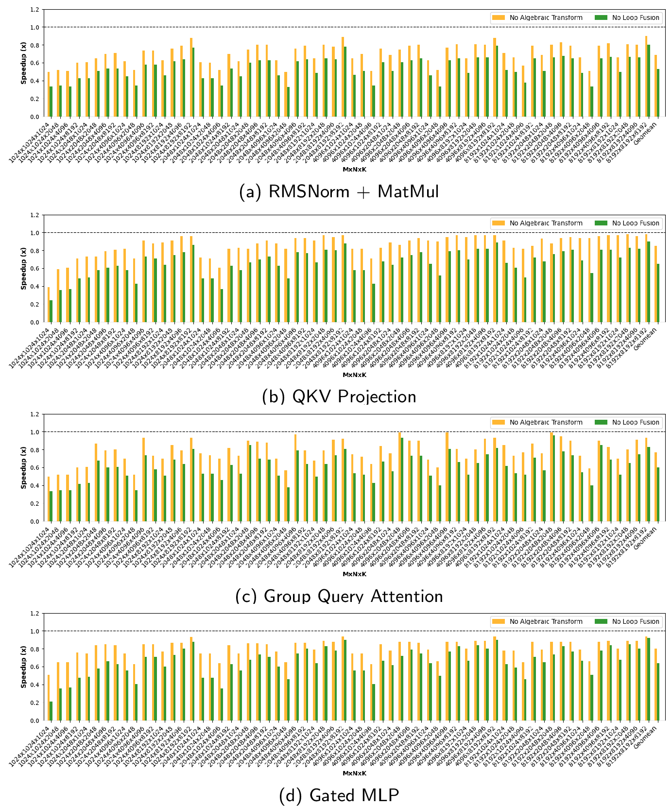
To understand the contribution of each optimization to performance, we selectively disable algebraic transformations and operator fusion, and measure the impact on four multi-operator benchmarks (Table 5). We do not disable tiling because it is required for executing kernels with large tensors that do not fit in the on-chip buffers. As discussed in Section 6.2, the individual operator benchmarks (Table 3) primarily demonstrate the impact of tiling, since single-operator kernels have limited opportunities for algebraic transformations or inter-operator fusion.
Operator fusion is the most impactful optimization. Across all four benchmarks, disabling fusion causes the largest performance degradation, with geomean slowdowns of 35–50%. Without fusion, intermediate results between operators must be written to and read back from HBM, significantly increasing memory traffic.
Algebraic transformations provide consistent gains. Disabling algebraic transformations leads to geomean slowdowns of 15–35% across the benchmarks. The impact is present across all four benchmarks, confirming that the graph mutator’s operator reordering contributes to performance even when fusion is still enabled.
The two optimizations are complementary. The combined effect of both optimizations (i.e., the full Axon pipeline) consistently outperforms either optimization alone, indicating that algebraic transformations and fusion target different sources of inefficiency: algebraic transformations expose parallelism and reduce unnecessary computation; fusion reduces memory traffic between operators.
| No Algebraic Transform | No Loop Fusion | |||||
|---|---|---|---|---|---|---|
| 2-4 (lr)5-7 Benchmark | Min | Max | Geomean | Min | Max | Geomean |
| RMSNorm+MatMul | 0.50x | 0.90x | 0.65x | 0.33x | 0.80x | 0.53x |
| QKV Projection | 0.39x | 0.98x | 0.85x | 0.24x | 0.90x | 0.65x |
| Group Query Attention | 0.50x | 0.98x | 0.77x | 0.34x | 0.96x | 0.60x |
| SiLU MLP | 0.51x | 0.94x | 0.80x | 0.21x | 0.92x | 0.64x |
6.5 RQ4: Compilation Overhead↩︎
Table 6 reports the compilation overhead for all benchmarks.
Phase 1 (Lowering and Emission): The full Axon pipeline—graph mutation, tiling, ISA synthesis, ISA fusion mutation, and NKI code emission—transforms the input computation graph and emits multiple candidate NKI programs.
Phase 2 (Compilation and Execution): Each emitted NKI program is compiled by the Neuron compiler backend and, if compilation succeeds, executed on Trainium. The best-performing kernel is selected.
Table 6 reports, for each benchmark, the number of graph-level operations (# Ops), the Phase 1 time, the number of emitted and compilable NKI programs, the Phase 2 time, and the total time. Note that # Ops counts operations after decomposition: a single high-level operator such as RMSNorm decomposes into multiple graph operations (square, mean, rsqrt, multiply), so # Ops can exceed 1 even for individual operator benchmarks. Not all emitted programs are compilable: as described in Section 4.6, Axon does not directly control on-chip buffer allocation, so candidates that satisfy Axon’s symbolic tile constraints may still be rejected by the Neuron compiler when the cumulative size of live tiles in a block exceeds the physical SBUF capacity.
Phase 1 is fast; Phase 2 dominates compilation time. Phase 1 completes in under 82 seconds even for the most complex kernels, as it operates symbolically on the computation graph. Phase 2, which involves parallelized compilation and serialized execution of NKI kernels on hardware, accounts for over 97% of total compilation time. Its cost is proportional to the number of compilable NKI kernels: element-wise and reduction operators produce 456–1,126 compilable kernels and complete Phase 2 in 289–348 seconds; kernels involving matrix multiplication produce 5,000–18,982 compilable kernels and take 3,156–4,107 seconds; and complex LLM layers produce 18,450–19,934 compilable kernels and take 4,992–5,983 seconds.
The search space is driven by the number of operators, input dimensions, and hardware constraints. In general, more operators (# Ops) lead to more emitted candidates, since each operator introduces tiling configurations
and instruction choices that compose multiplicatively (Section 4.1). However, the number of input dimensions and hardware constraints also play a significant role. MatMul, despite being a single operator, emits
14,554 candidates—far more than other individual operators (625–1,475)—because its three input dimensions (M\(\times\)K\(\times\)N) create a larger combinatorial space for block size
exploration compared to the two dimensions of element-wise operators. Conversely, Transpose+MatMul (2 operators) emits only 8,050 candidates, fewer than MatMul alone, because the ISA Fusion Mutator (Section 4.5) eliminates redundant transpose instructions: lowering matmul introduces a transpose (required by nc_matmul’s semantics), which is fused with the
pre-existing transpose operation in the input graph, reducing the number of emitted candidates. Among multi-operator kernels, the search space grows with complexity but is bounded by hardware constraints: GQA (6 operators) and Gated MLP (5–7
operators) approach an upper bound of approximately 29,500 emitted candidates.
Not all emitted candidates are compilable. Across all benchmarks, 60–76% of emitted kernels are compilable (e.g., GQA: 19,627 of 28,219); the remainder are rejected by the Neuron compiler due to hardware resource constraints such as insufficient SBUF capacity (Section 4.6).
The compilation overhead is a one-time cost. The total time ranges from approximately 5 minutes for simple operators to 1.7 hours for the most complex kernels (SwiGLU Gated MLP); since performance depends only on tensor shapes, the optimized kernel is reused for all subsequent executions. This one-time search cost is comparable to that of other optimizing compilers that explore large search spaces: Mirage [8] reports search times of up to 4 hours on GPUs for similar LLM kernels, and schedule-based compilers such as Halide [11], AutoTVM [34], and Ansor [10] take several hours to explore tiling and fusion choices. In practice, kernels for commonly used tensor shapes can be compiled ahead of time and cached as artifacts for reuse across models—a standard practice at companies like Amazon to amortize compilation cost [35].
Appendix 9 discusses threats to validity, including end-to-end inference, generalizability beyond Trainium, and benchmark coverage.
| Kernel | # Ops | Phase 1 (s) | # Emitted | # Compilable | Phase 2 (s) | Total (s) |
|---|---|---|---|---|---|---|
| Tensor Multiply | 1 | 8.2 | 625 | 456 | 288.5 | 296.7 |
| Cumsum | 1 | 11.4 | 625 | 456 | 314.3 | 325.7 |
| RMSNorm | 5 | 15.6 | 900 | 540 | 348.2 | 363.8 |
| Softmax | 3 | 16.3 | 900 | 540 | 319.9 | 336.2 |
| ReLU | 1 | 9.6 | 625 | 456 | 290.5 | 300.1 |
| SiLU | 1 | 10.8 | 625 | 456 | 304.1 | 314.9 |
| GLU | 3 | 10.8 | 1,258 | 875 | 305.7 | 316.5 |
| SwiGLU | 3 | 10.9 | 1,258 | 875 | 308.9 | 319.8 |
| MaxPool | 1 | 22.7 | 1,475 | 1,126 | 324.5 | 347.2 |
| RoPE | 1 | 15.9 | 1,250 | 912 | 327.2 | 343.1 |
| MatMul | 1 | 24.8 | 14,554 | 9,532 | 3,228.6 | 3,253.4 |
| Transpose+MatMul | 2 | 29.3 | 8,050 | 5,000 | 3,155.7 | 3,185.0 |
| RMSNorm+MatMul | 6 | 37.1 | 17,500 | 12,750 | 3,246.4 | 3,283.5 |
| MatMul+Add+RMSNorm | 7 | 39.4 | 19,500 | 14,758 | 3,253.7 | 3,293.1 |
| Softmax+MatMul | 4 | 31.9 | 16,263 | 12,549 | 3,242.4 | 3,274.3 |
| MM+MM+SiLU+Mul | 4 | 75.4 | 27,740 | 18,982 | 4,106.8 | 4,182.2 |
| QKV Projection | 3 | 68.2 | 26,750 | 18,450 | 5,878.9 | 5,947.1 |
| Group Query Attention | 6 | 79.4 | 28,219 | 19,627 | 4,992.2 | 5,071.6 |
| SiLU Gated MLP | 5 | 81.6 | 29,535 | 19,934 | 5,949.3 | 6,030.9 |
| SwiGLU Gated MLP | 7 | 79.8 | 29,535 | 19,934 | 5,982.8 | 6,062.6 |
7 Related Work↩︎
Algebraic transformation compilers. TASO [5], PET [7], Grappler [36], and EinNet [37] optimize tensor programs by rewriting computation graphs using algebraic equivalences: TASO enumerates user-provided rewrite rules with random testing, and PET adds partially equivalent rewrites with correction kernels. Equality saturation-based compilers (e.g., Tensat [6], Constable [14]) apply hand-written Egg [22] rewrite rules but provide no semantic correctness guarantees; overall, these methods rely on pattern-specific rules and do not automatically reason about operator semantics. The closest prior work to Axon is Mirage [8], which uses probabilistic equivalence checking to jointly optimize algebraic and scheduling transformations on \(\mu\)Graphs and relies on hand-written NKI templates to constrain search for Trainium. In contrast, Axon discovers transformations using operator propagation, synthesizes ISA instructions from specifications, and proves correctness with SMT over unbounded tensors, without hand-written rewrite rules or templates.
Schedule-based compilers. Halide [11] introduced the idea of separating the algorithm from its schedule; TVM [9], Ansor [10], and others [38]–[40] build on this idea to search for optimized schedules (tiling, fusion, parallelization) on CPUs and GPUs. However, these compilers target CPUs and GPUs—none currently generates code for tile-based AI accelerators. Axon jointly explores algebraic transformations and schedule transformations (tiling, fusion) for tile-based accelerator programs, whereas schedule-based compilers only explore schedules for a fixed algorithm.
Synthesis-based compilers. Works such as Rake [41], Pitchfork [42], Hydride [43] and Misaal [44] use program synthesis to synthesize for x86 [45], ARM [46], and Hexagon DSP [47] vector ISA; Diospyros [48] targets Tensilica DSP’s vector ISA. However, all of these works only target 1-D vector instructions. Hardboiled [49] uses equality saturation in Halide [11] to target 2-D Intel AMX [45] and Nvidia Tensor Core [50] ISA for signal and image processing; however, it only lowers to matrix multiply and accumulate operations. Whereas prior works on guided tensor program lifting [51], [52] synthesize higher-level abstractions from legacy C/C++ code, without synthesizing complex tensor operations, Axon synthesizes 2-D tile instructions with hardware-constrained tile dimensions. Tile-based accelerator languages. Vendors provide tile-based kernel languages for their accelerators: NKI [1] for Amazon’s Trainium, Pallas [2] for Google’s TPUs, and Triton [3] for GPUs. Higher-level frameworks such as Hidet [53], TileLang [18], and Helion [54] compile from high-level tensor programs to GPU kernels. All of these require programmers to have knowledge of hardware-specific details. Axon takes a high-level NumPy-like program and automatically generates optimized code in NKI, without requiring programmers to have hardware expertise.
Verified tensor transformations. Liu et al. [55] present a Coq framework that verifies scheduling rewrites (tiling, fusion, compute_at) for Halide programs via machine-checked proofs. TensorRight [15] provides an SMT-based framework for verifying XLA [56] rewrite rules over unbounded tensors. NiceToMeetYou [57] uses synthesis with SMT-based verification to generate sound abstract transformers for LLVM [58] static analyses from MLIR [23] semantics. Axon uses SMT-verified algebraic transformations and ISA instruction selection for AI accelerators.
8 Conclusion↩︎
We introduced Axon, a synthesizing superoptimizer that automatically generates optimized tile-based AI accelerator kernels from high-level tensor programs, combining provably correct algebraic transformations, ISA synthesis, tiling, and fusion in a unified \(\nu\)Graph representation. On Amazon’s Trainium across 20 benchmarks, Axon achieves speedups up to 3.7x on individual operators and up to 19x on multi-operator kernels over the Neuron compiler, up to 1.35x over hand-optimized NKI kernels, and geomean speedups of 2–10% over Mirage on all benchmarks it supports.
9 Threats to Validity↩︎
9.0.0.1 End-to-end inference.
Our evaluation measures kernel-level performance, consistent with Mirage [8] and other kernel optimization work. End-to-end inference latency depends on additional factors such as kernel launch overhead, collective communication, and framework-level scheduling, which are orthogonal to the kernel optimizations presented in this paper.
9.0.0.2 Generalizability beyond Trainium.
Axon’s core algorithms—algebraic transformations, tiling exploration, ISA synthesis, and fusion—could be adapted to other tile-based accelerators with similar architectural properties (Section 3). Targeting a new platform requires providing new ISA semantics, hardware constraints, and a code emitter; the synthesis pipeline itself remains unchanged. Accelerators with fundamentally different execution models (e.g., many-core architectures, GPU thread-block models) are not directly targeted by Axon’s current design.
9.0.0.3 Hardware generation.
We evaluate on first-generation Trainium due to limited public availability of newer generations (Trainium2 [59] and Trainium3 [60]). Based on published architecture descriptions, all Trainium generations share the same multi-engine design, NKI programming model, and tile-based execution model, so we expect Axon’s optimizations to transfer, though specific tiling parameters and performance characteristics may differ.
9.0.0.4 Benchmark coverage.
Our benchmark suite covers core operators and multi-operator kernels, including LLM-specific layers such as GQA and Gated MLP, and overlaps significantly with Mirage’s evaluation. However, it does not cover all kernel types, such as convolutions, sparse operators, or training-specific kernels like backward passes.
10 Additional Algebraic Transformation Examples↩︎
10.1 Softmax+MatMul↩︎
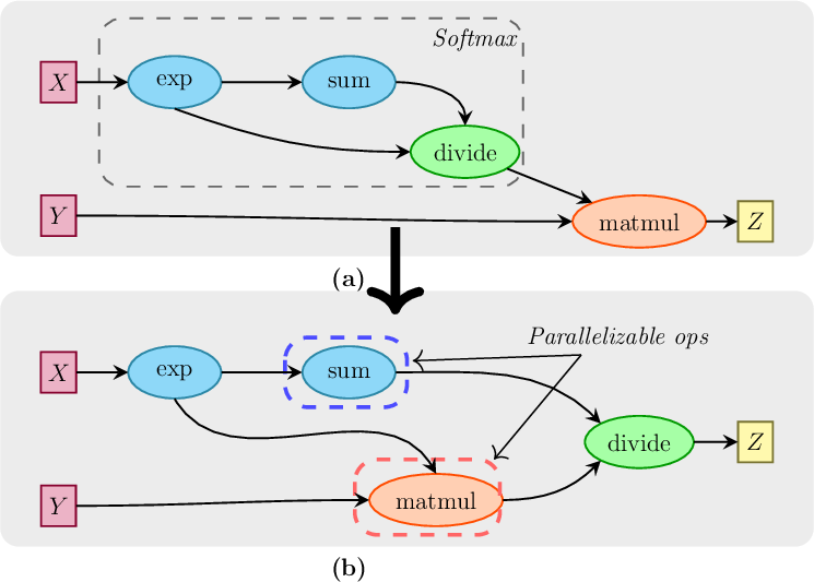
Figure 16 shows a Softmax+MatMul kernel where the divide and matmul operators can be reordered so that matmul executes on the Tensor Engine while the row-wise
sum reduction executes on the Vector Engine in parallel, rather than sequentially.
This transformation is analogous to the RMSNorm+MatMul rewrite discussed in Section 2: an element-wise operation (here, divide by the softmax normalization factor) commutes with matmul
because the normalization factor reduces along the same dimension contracted by the matrix multiplication.
Axon automatically discovers this transformation through operator propagation and provably checks it using SMT over unbounded tensors (Section 5). However, existing graph rewriting systems—including TASO [5], Tensat [6], Constable [14], and Mirage [8]—do not support this rewrite because their hand-written rules do not cover this particular pattern of operator reordering. This illustrates the fundamental limitation of pattern-matching approaches: they can only perform transformations for patterns that have been manually anticipated and implemented.
11 Ablation Study: Per-Dimension Results↩︎
Figure 17 shows the per-dimension results for the ablation study discussed in Section 6.4. Each bar shows performance relative to Axon with all optimizations enabled (dashed line at 1.0x).
12 Generated NKI Kernel for RMSNorm+MatMul↩︎
Figure 18 shows the NKI kernel generated by Axon for the RMSNorm+MatMul input program from Figure 2. The RMS branch (lines 18–21) executes on the Vector/Scalar Engine while the MatMul branch (lines 24–39) executes on the Tensor Engine in parallel within the same loop nest. The results are combined at the end (lines 46–49), reflecting the algebraic transformation from Figure 3 (b).
None
Figure 18: NKI kernel generated by Axon for RMSNorm+MatMul from the 5-line input in Figure 2..