Scaling Nonlinear Optimization: Many Problems One GPU
June 24, 2026
Abstract
Many robotics problems, including trajectory optimization, inverse kinematics, and contact-rich motion planning, reduce to nonlinear programs (NLPs). Mature NLP solvers such as IPOPT can solve these problems, offering hard constraint satisfaction,
optimality guarantees, and favorable scaling with problem dimension. These solvers underpin gradient-based methods in robotics, yet remain CPU-bound and solve only one problem at a time, preventing their integration into GPU-batched learning pipelines. On
the other hand, sampling-based approaches such as reinforcement learning, model predictive path integral, and imitation learning have become the core of modern robotics research due to their ability to leverage GPU-batched simulators. These simulators can
generate orders of magnitude more dynamics rollouts per second than was previously possible. If a GPU-batched NLP solver existed, it would unlock similar speedups in the number of constrained, locally optimal solutions generated per second. This regime of
solving many problems concurrently versus solving a single problem at a time is a key requirement for integrating NLP solvers in modern GPU-batched robotics frameworks. To this end, we introduce jaxipm, the first GPU-batched NLP solver, based
on IPOPT, and implemented in JAX. We accomplish this by redesigning IPOPT’s algorithm to eliminate control flow with heterogeneous iteration fusion, and by minimizing GPU idle time with iteration level batching. We evaluate
jaxipm on a variety of quadrotor nonlinear model predictive control benchmarks, including reference tracking in the presence of obstacles, multi-quadrotor navigation without collision, and navigation in a cluttered environment. We demonstrate
up to a \(32.85\times\) increase in throughput over IPOPT. Our complete open-source codebase is available at https://github.com/johnviljoen/jaxipm.
1 Introduction↩︎
Many core problems in robotics, such as trajectory optimization, inverse kinematics, and contact-rich manipulation, reduce to nonlinear programs (NLPs) [1]–[4]. Two broad approaches solve these problems: sampling-based (SB) methods, such as reinforcement learning (RL), model predictive path integral control (MPPI) [5], and the cross-entropy method [6]; and gradient-based (GB) methods, which use mature, well-tested, CPU-based optimizers such as IPOPT [7], KNITRO [8], and SNOPT [9]. In recent years, GPU-batched simulators [10]–[12] have driven SB methods to dominance by generating synthetic data orders of magnitude faster than classical CPU-based alternatives.
Despite this shift, GB methods offer several advantages over SB methods [13]. For instance, GB methods enforce hard constraints directly and converge to solutions satisfying optimality conditions, whereas SB methods encode constraints as soft penalties, providing neither feasibility nor optimality guarantees. GB methods also scale well with problem dimension and exploit model information to refine solutions to arbitrary precision. By contrast, SB methods require exponentially more samples as state and action dimensions grow and cannot improve beyond the resolution of their samples [13], [14]. However, GB methods carry their own limitations. They typically require known twice-differentiable dynamics models and struggle to execute in real time, both areas of active research [15]–[17]. Most critically, NLP optimizers used in GB methods remain CPU-bound, preventing their integration into modern GPU-batched robotics workflows. Generating dataset-scale collections of solutions stalls at single-process throughput, and inside any larger GPU pipeline, the optimizer becomes the slowest link, throttling the entire batch to a single problem at a time while the rest of the GPU sits idle. As a result, GB methods miss the orders-of-magnitude parallelism speedups that drove SB methods to dominance.
To bridge this gap, we introduce jaxipm, a first-of-its-kind, open-source, GPU-batched NLP optimizer. We base jaxipm on IPOPT [7],
one of the most widely used NLP optimizers [18]–[21]. We chose IPOPT for its broad applicability
to NLPs and its robustness, which together have made it the default in much of the robotics and engineering community. IPOPT solves an NLP through a sequence of iterations, each of which may resort to a variety of fallbacks for known edge cases. This
machinery underlies IPOPT’s robustness, but poses unique challenges for GPU-based execution. Within a batch, every problem can take a different control flow branch at each iteration and terminate at a different iteration count. This conflicts with the
uniform execution model that GPUs rely on for parallelism. We get around this issue in jaxipm with our two contributions.
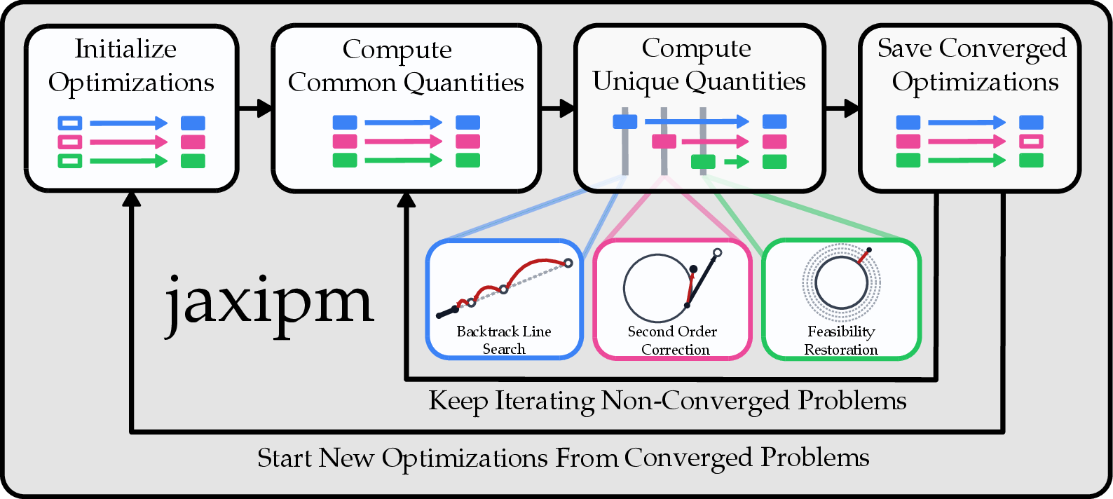
The first is heterogeneous iteration fusion, where we rework every possible fallback into one iteration type. This means that where IPOPT would have computed different control flow branches conditioned on the optimization state, we instead compute the same thing for every iteration without sacrificing any benefits IPOPT gained from its control flow. Our key insight is that most of IPOPT’s control flow branches share a common set of expensive computations, meaning that we can compute these shared computations concurrently across an entire batch. For the small remainder of truly unique computations, we run them for all problems regardless of the branch IPOPT would have taken, and select the correct output afterward.
The second is iteration level batching, where we hot-restart finished optimization problems without interrupting ongoing ones to minimize GPU downtime. A naive parallel implementation would batch at the solve level, requiring every problem to
complete before the next batch can begin and leaving the GPU idle until the slowest solve finishes. To minimize this idling, we designed jaxipm around finer-grained iteration level batching, which synchronizes at iteration boundaries and lets
completed problems be replaced with new ones mid-batch while unfinished problems continue iterating.
We wrote jaxipm in JAX [22], both to achieve high performance and to allow for native interoperability with GPU-batched learning frameworks used in
modern robotics research [10]–[12].
We evaluate jaxipm on three different quadrotor Nonlinear Model Predictive Control (NMPC) benchmarks, namely single-quadrotor navigation, multi-quadrotor consensus, and reference tracking with time-varying obstacles, where we achieve up to
\(32.85\times\) throughput acceleration over IPOPT. We also demonstrate bit-parity with IPOPT on a per-iteration level across an optimization that utilizes most of IPOPT’s control flow branches.
Our Contribution: We present jaxipm, the first GPU-batched NLP solver, capable of solving thousands of NLPs concurrently through heterogeneous iteration fusion and iteration level batching.
2 Related Works↩︎
NLP solvers. Decades of work have produced mature NLP solvers that implement sequential quadratic programming (SNOPT [9]) and interior point methods (IPOPT [7]), with hybrid implementations such as KNITRO [8] supporting both. These solvers handle general equality and inequality constrained problems, scale to thousands of variables, and provide convergence guarantees that have made them the backbone of model-based robotics and engineering optimization [18]–[21], [23]. However, SNOPT, IPOPT, and KNITRO all target the CPU and execute their iterations sequentially.
GPU acceleration of NLP solvers. A recent line of work now targets IPOPT-like solvers by porting their dominant per-iteration cost onto the GPU. These are: the solution of a highly sparse symmetric indefinite linear system known as the KKT system, and the sparse derivative evaluation that constructs that linear system. HyKKT [24] was the first to apply a positive-definite reformulation of the indefinite KKT system as a GPU-acceleration strategy for general NLPs. MadNLP [25] reimplements IPOPT in Julia and achieves GPU acceleration in two ways. Firstly, it supports its own positive-definite KKT system reformulation [26] solved by GPU-accelerated linear solver cuDSS [27]. Secondly, MadNLP accelerated the evaluation of sparse derivatives through ExaModels [25]. Despite achieving GPU-acceleration, MadNLP does not achieve GPU-batching as its algorithmic logic, including its control flow branches, remains CPU-bound.
Batched convex solvers. Another line of work is GPU-batched solvers for convex optimization problems, which do not require the control flow branches that kept NLP solvers CPU-bound. A number of approaches have been used for these, such as interior-point methods [28]–[30], primal-dual hybrid-gradient methods [31], and operator-splitting methods [32]. None of them, however, extends to NLPs, leaving applications with nonlinear dynamics or constraints without a batched GPU solver.
Demand for batched NLP data generation. Recent robotics research reveals a growing demand for large datasets of high-quality optimization solutions. Opt2Skill [33] trains humanoid RL policies on reference trajectories that an optimizer generates offline, showing that model-based optimization produces better training data than human demonstrations or inverse kinematics baselines.
In [34], the authors take the same approach for legged locomotion, distilling an MPC controller into a quadruped policy via
behavior cloning, where every demonstration in the training set is an NLP solution. In [35], the authors argue
more broadly that closing the robot learning data gap requires hybrid pipelines combining model-free learning with model-based optimization at scale. These works point to the same bottleneck: no current solver produces NLP solutions at the scale these
pipelines demand. We aim to close this gap with jaxipm, which runs thousands of solves concurrently on a GPU.
3 Problem Statement↩︎
In this section, we define our notation used in this paper, the class of optimization problems that we target, and the batched generalization that our optimizer jaxipm is designed to solve. We first introduce a parametric nonlinear program,
and then describe a batch as a collection of such programs that share the same structure but differ in their internal parameters.
Notation. The \(i\)-th row of a matrix \(M \in \mathbb{R}^{n\times m}\) is written as \(M_i\). The \(i\)-th element of a vector \(v \in \mathbb{R}^n\) is written as \(v^{(i)}\). We define the \(\text{diag}\) operator on a vector \(v \in \mathbb{R}^n\) as the diagonal matrix \(\text{diag}(v) \in \mathbb{R}^{n \times n}\) with \(v\) on its diagonal, and zeros elsewhere. We also define \(e\) as the vector of all ones for the appropriate dimension, as well as \(n_x\) and \(n_c\) to be the number of primal optimization variables and equality constraints, respectively.
Single instance. We consider parametric nonlinear programs of the form:
\[\tag{1} \begin{align} \min_{x\in \mathbb{R}^{n_x}} \quad & f(x, \theta) \tag{2} \\ \text{s.t.} \quad & c(x, \theta) = 0 \tag{3} \\ & x_L \leq x \leq x_U. \tag{4} \end{align}\]
where \(x \in \mathbb{R}^{n_x}\) is the decision variable, and \(\theta \in \mathbb{R}^{n_\theta}\) is a parameter vector that defines the optimization problem, where \(n_\theta\) is the number of parameters. Here, \(f \colon \mathbb{R}^{n_x} \times \mathbb{R}^{n_\theta} \to \mathbb{R}\) is the objective, \(c \colon \mathbb{R}^{n_x} \times \mathbb{R}^{n_\theta} \to \mathbb{R}^{n_c}\) collects the equality constraints, and \(x_L, x_U \in \mathbb{R}^{n_x}\) are elementwise lower and upper bounds on \(x\). We assume \(f\) and \(c\) are twice continuously differentiable in \(x\) for every \(\theta\) of interest. Note that general inequality constraints can also be included in this formulation through slack variables.
Batched instances. A batch collects \(N\) instances of problem 1 that share the functions \(f\) and \(c\) and the bounds \(x_L\), \(x_U\), and that differ only in the parameter \(\theta\). We write the decision variable and parameter of the \(i\)-th instance as \(X_i \in \mathbb{R}^{n_x}\) and \(\Theta_i \in \mathbb{R}^{n_\theta}\), respectively. Here, \(X \in \mathbb{R}^{N \times n_x}\) is the stack of decision variables for the batch, and \(\Theta \in \mathbb{R}^{N \times n_\theta}\) is the stack of parameters for the batch. We can now define the batched problem:
\[\begin{align} \min_{X_i \in \mathbb{R}^{n_x}} & \; f(X_i, \Theta_i) \\ \text{s.t.} & \; c(X_i, \Theta_i) = 0 \\ & \; X_{i_L} \leq X_i \leq X_{i_U}, \end{align} \qquad i = 1, \dots, N \label{eqn:nlp95batch95naive}\tag{5}\]
where each row \(X_i\) is solved as an independent program. Here, \(X_{i_L}\) and \(X_{i_U}\) are the lower and upper bounds for the \(i\)-th instance, which equal the shared bounds \(x_L\) and \(x_U\) for every \(i\). Instances are decoupled in their decision
variables, so a batch of \(N\) programs is mathematically equivalent to \(N\) separate calls to a single instance solver. Our solver jaxipm is built to exploit this structure on
GPU hardware by adapting IPOPT, the most widely used solver for problems of the form 1 . We review the IPOPT algorithm in the next section before detailing our contribution.
4 IPOPT Background↩︎
In this section, we provide a brief background to IPOPT for solving 1 and explain why it cannot trivially scale to solve 5 . We first introduce how it calculates step directions, then its techniques for handling edge cases throughout its optimization, and finally explain why this makes it ineffective at solving the batched problem 5 . When solving 1 , for simplicity, we assume that every \(x^{(i)}\) is upper and lower bounded by \(x_L^{(i)}\), \(x_U^{(i)}\)4. Since the parameters \(\theta\) are fixed within a single solve, we suppress them and write \(f(x)\) and \(c(x)\) for \(f(x, \theta)\) and \(c(x, \theta)\).
Prerequisites. IPOPT is a primal-dual interior-point method. Like [36]–[38], it enforces the bound constraints 4 with a logarithmic barrier, forming the barrier objective:
\[\varphi_\mu(x) := f(x) - \mu \sum_{i=1}^{n_x} \ln (x^{(i)} - x_L^{(i)}) - \mu \sum_{i=1}^{n_x}\ln(x_U^{(i)} - x^{(i)}), \label{eqn:barrier95obj}\tag{6}\]
with barrier parameter \(\mu > 0\), and solves a sequence of barrier problems while driving \(\mu\) to zero [7]. It maintains a primal-dual iterate \((x, y_c, z_L, z_U)\) where \(y_c\), \(z_L\) and \(z_U\) are the Lagrange multipliers for 3 , the lower bounds, and the upper bounds of 4 , respectively. We write the Lagrangian as:
\[\mathcal{L}(x, y_c, z_L, z_U) := f(x) + y_c^\top c(x) - z_L^\top (x - x_L) - z_U^\top (x_U - x). \label{eqn:barrier95lagrangian}\tag{7}\]
For convenience, let \(W := \nabla_{xx}^2 \mathcal{L}(x, y_c, z_L, z_U)\) denote the Lagrangian Hessian and \(A := \nabla c(x)\) the constraint Jacobian, and write \(S_L := \text{diag}(x - x_L)\), \(S_U := \text{diag}(x_U - x)\), \(Z_L := \text{diag}(z_L)\), and \(Z_U := \text{diag}(z_U)\). All references to “iterate" henceforth refer to the primal-dual iterate \((x, y_c, z_L, z_U)\).
Step direction. At each iteration, IPOPT computes a search step from the following optimality conditions for the barrier subproblem:
\[\tag{8} \begin{align} \nabla f(x) + \nabla c(x)^\top y_c - z_L + z_U & = 0 \tag{9} \\ c(x) & = 0 \tag{10} \\ S_L z_L - \mu e & = 0 \tag{11} \\ S_U z_U - \mu e & = 0, \tag{12} \end{align}\]
where 9 is \(\nabla_x \mathcal{L}(x, y_c, z_L, z_U) = 0\), 10 is \(\nabla_{y_c} \mathcal{L}(x, y_c, z_L, z_U) = 0\), and 11 12 represent the relaxed complementarity conditions for the two bounds. Note that equations 8 for \(\mu=0\) together with \(z_L, z_U \geq 0\), and \(x_L \leq x \leq x_U\) are the KKT conditions for the original problem 1 5. To compute the step, IPOPT applies Newton’s method to 8 . The Newton system for the step \((\Delta x, \Delta y_c, \Delta z_L, \Delta z_U)\) is:
\[\setlength{\arraycolsep}{3pt} \begin{bmatrix} W & A^\top & -I & I \\ A & 0 & 0 & 0 \\ Z_L & 0 & S_L & 0 \\ -Z_U & 0 & 0 & S_U \end{bmatrix} \begin{bmatrix} \Delta x \\ \Delta y_c \\ \Delta z_L \\ \Delta z_U \end{bmatrix} = -\begin{bmatrix} \nabla_x \mathcal{L}(x, y_c, z_L, z_U) \\ c(x) \\ S_L z_L - \mu e \\ S_U z_U - \mu e \end{bmatrix}. \label{eqn:newton95full}\tag{13}\]
The last two rows of 13 give \(\Delta z_L = S_L^{-1}(\mu e - S_L z_L - Z_L \Delta x)\) and \(\Delta z_U = S_U^{-1}(\mu e - S_U z_U + Z_U \Delta x)\), which we substitute into the first row to eliminate the bound-multiplier steps. This substitution produces \(\Sigma := S_L^{-1} Z_L + S_U^{-1} Z_U\), and collapses the first right-hand side to the barrier gradient \(\nabla \varphi_\mu(x) = \nabla f(x) - \mu\, S_L^{-1} e + \mu\, S_U^{-1} e\). This forms the following “augmented" system eq. ¿eq:eqn:augmented95kkt? , which produces the”augmented" step \((\Delta x, \Delta y_c)\) when solved6.
\[\begin{bmatrix} W + \Sigma & A^\top \\ A & 0 \end{bmatrix} \begin{bmatrix} \Delta x \\ \Delta y_c \end{bmatrix} = -\begin{bmatrix} \nabla \varphi_\mu(x) + A^\top y_c \\ c(x) \end{bmatrix}. \label{eqn:augmented95kkt}\tag{14}\]
IPOPT solves a system of the form 14 by computing a symmetric indefinite factorization \(LDL^\top\) of the left-hand side matrix, from which the step \((\Delta x, \Delta y_c)\) is obtained. This serves a purpose beyond finding the step; the factorization reports the matrix inertia, the triple \((n_+, n_-, n_0)\) counting its positive, negative, and zero eigenvalues. For the step to be a descent direction on the barrier objective, the matrix must have inertia \((n_x, n_c, 0)\), that is, \(n_x\) positive and \(n_c\) negative eigenvalues and no zero eigenvalues [39]. The matrix in 14 may not satisfy this, and so IPOPT can add perturbation terms \(\delta_x I\) and \(-\delta_c I\) with \(\delta_x, \delta_c \geq 0\) to the top-left and bottom-right diagonal blocks, respectively, such that the inertia requirement is satisfied.
The factorization of 14 dominates the per-iteration cost, and so its efficiency governs the wall-clock time of the entire solve. Because of this, in our method, we have focused on making this factorization as fast as possible on GPU hardware.
Edge case handling. The Newton step from 14 may be a poor choice for a number of reasons. This is why IPOPT has several fallback mechanisms for common failure modes, which we list in Table 1. For example, row (1) of Table 1 asks: What if the trial (Newton step) is rejected? This typically means that the landscape of the optimality conditions 8 is rapidly changing, and so the linearization used to form 14 is only locally accurate. To combat this, the size of the step is reduced according to a backtracking scheme, bringing the step closer to where the linearization was accurate. Similarly, there are other failure modes with designed fallbacks that we provide some intuition for in Table 1.
| Question | Branch |
|---|---|
| (1) What if the trial is rejected? | Backtracking line search shortens the step along the Newton direction and retests. |
| (2) What if the linearization at the current iterate disagrees with the constraints at the trial? | A second order correction changes the step direction based on information gathered at the original trial. |
| (3) What if a short run of rejections is hiding longer-horizon progress? | The watchdog accepts a small sequence of trial steps unconditionally, either accepting the resultant iterate, or reverting to the entry iterate. |
| (4) What if the step is already too small for backtracking to refine? | A tiny-step rule accepts it unconditionally. |
| (5) What if repeated rejections suggest infeasibility? | Soft feasibility restoration changes the acceptance criteria, and continues until original criteria are fulfilled or an iteration limit is reached. |
| (6) What if the iterate cannot make progress on the original problem? | Hard feasibility restoration solves a new problem whose objective is the constraint violation, returning once an acceptable point is found (which itself contains another copy of every control flow branch in this table, including a nested hard feasibility restoration). |
| (7) What if our barrier parameter \(\mu\) adaptations seem too aggressive? | Switch from an adaptive rule that reacts to the current iterate to a monotone schedule that decreases \(\mu\) once the current subproblem converges. |
Why is IPOPT hard to batch? What we have spoken about so far is how IPOPT goes about solving a single problem. Now, if we want to solve multiple problems concurrently, as is the case in 5 , IPOPT could not select different control flow branches (Table 1) for different problems. This is because IPOPT’s control flow assumes a single iterate, so a naive batch would have to force every member onto the same branch each step. At best, this would inflate iteration counts; at worst, it would cause individual solves to fail. Retaining independent branching with IPOPT therefore requires solving 1 sequentially over \(\Theta\).
5 Batched Interior Point Method↩︎
In this section, we will describe how we rebuilt IPOPT from scratch to enable high throughput batch solving whilst maintaining per-optimization control flow. We will go over how we fused all control flow branches via heterogeneous iteration fusion, and then how we accelerated throughput via iteration level batching.
Heterogeneous iteration fusion. We could not use IPOPT to directly solve 5 effectively because we could not select different control flow branches for \(X_i\) and
\(X_j\) for \(i \neq j\). This means that even when \(X_i\) and \(X_j\) would benefit from different control flow branches,
which we call heterogeneous iterations, they would not be able to. This problem would be solved if we could somehow remove all control flow branches so that every optimization in the batch always did the same operation. We have done exactly this in
jaxipm by walking through each control flow branch in Table 1 and splitting its work into two parts: computation that is shared across branches and computation that is unique to branches. Shared work is computed
once per iteration. For the remaining branch-unique work, we compute all branches for all optimizations and select from the outputs based on which branch was taken. For example, consider the situation where \(X_i\) and
\(X_j\) wish to perform a second order correction, and a backtracking line search, respectively. The second order correction and the backtracking line search require additional linear solves and scalar-vector
multiplications, respectively. In this example, we will compute the linear solves and the scalar-vector multiplications for both \(X_i\) and \(X_j\). Although neither \(X_i\) nor \(X_j\) requires the computation of both branches, doing this ensures that both optimizations perform the same computation. The result of this is an optimizer that takes
heterogeneous iterations and fuses them into a single iteration body that is identical for all members. Because every iteration is now the same computation, an entire batch of NLPs can advance in lockstep.
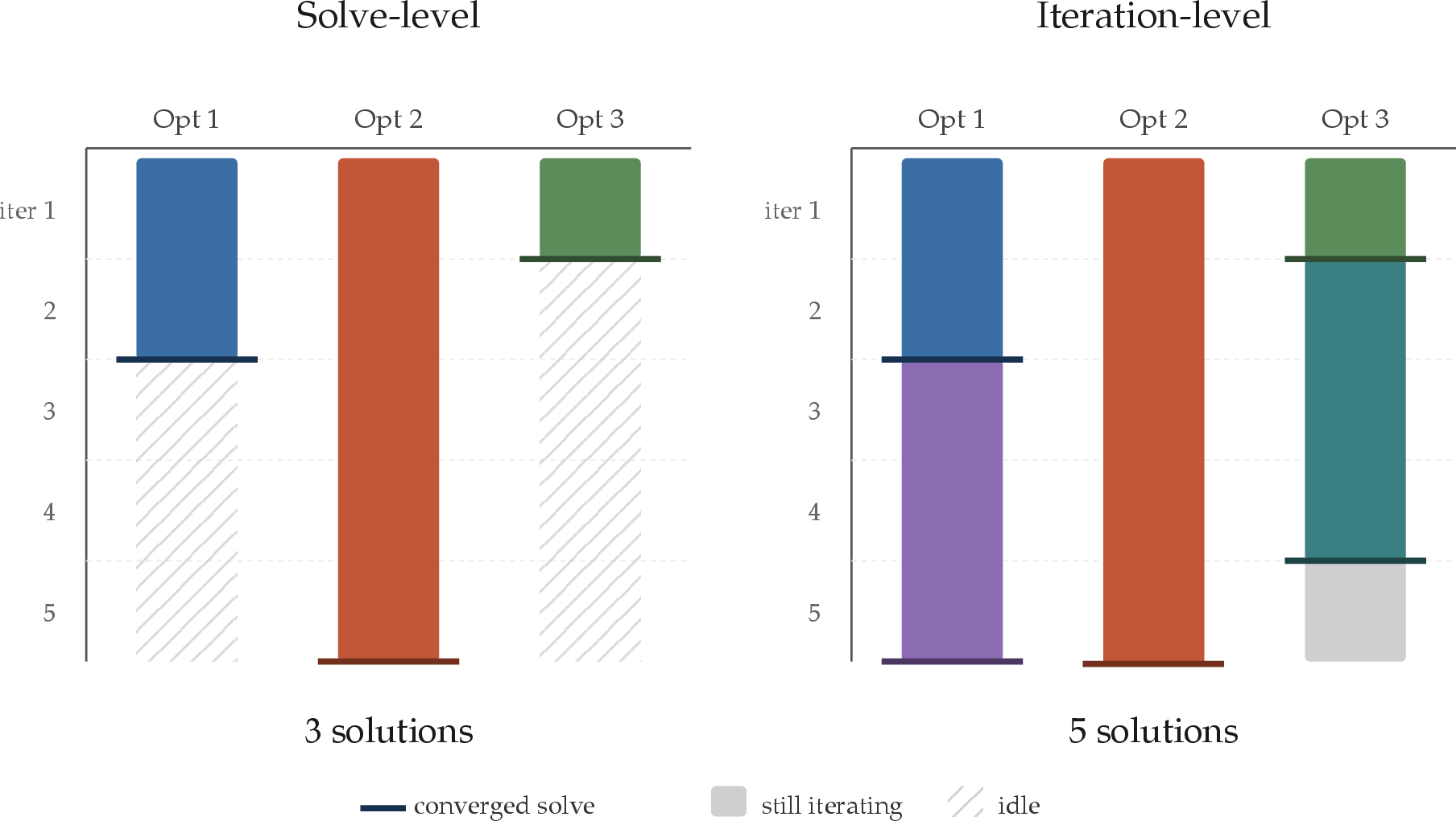
Iteration level batching. While effective, what we have discussed so far still leaves one inefficiency: the batch only advances as fast as its slowest member. If one problem converges in 10 iterations and another 100, then the faster problem must wait for the slower one to complete before the next batch can begin. Rather than letting the throughput of our batch optimizer be determined by the pace of its slowest member, upon convergence of one member, we hot-restart a new optimization in its place. When a member converges, we initialize a fresh problem in its place on the next iteration, while all other members continue iterating uninterrupted. See Figure 2 for a graphical illustration of this. This means that we batch at the iteration level rather than the solve level.
6 Results↩︎
In this section, we will outline our results. We create three NMPC scenarios designed to demonstrate our optimizer jaxipm on robotics scenarios. We first demonstrate raw throughput, and the benefit of iteration level batching.
Then, we test scalability both in terms of difficulty and dimensionality. Finally, we evaluate correctness against IPOPT.
We use quadrotors in all of these experiments due to their nonlinear, smoothly second order differentiable dynamics. We consider 13 DoF quadrotors whose state \(x = (p, q, v, \omega) \in \mathbb{R}^3 \times \mathbb{R}^4 \times \mathbb{R}^3 \times \mathbb{R}^3\), stacks position, attitude quaternion, and body linear and angular velocities. The dynamics \(\dot{x} = f(x,u)\) combine standard quadrotor translational and rotational kinematics [40] with four rotor angular velocity inputs \(u \in \mathbb{R}^4\). In all tests, we use NMPC to perform trajectory optimization on quadrotors with a timestep of 0.1s and a prediction horizon of 30. This means that each quadrotor optimization has a minimum of 506 optimization variables, excluding slacks from inequality constraints.
Although the quadrotor represents a small fraction of robotics problems our general-purpose NLP optimizer can handle, it is sufficient to demonstrate the benefits of our contributions in this paper: iteration level batching and heterogeneous iteration fusion. We also demonstrate algorithmic parity with IPOPT, and therefore claim that our method can be used wherever IPOPT has been used before. With this in mind, we have designed a set of experiments centered around quadrotors that stress test throughput, scalability, and correctness.
We compare against CasADi/IPOPT [7], [18] and ExaModels/MadNLP [25]. MadNLP is a GPU-accelerated version of IPOPT that utilizes cuDSS as its linear solver, the same as jaxipm. Specifically, MadNLP accelerates the linear
solves of 14 with cuDSS, and accelerates the evaluation of sparse derivatives using ExaModels. Crucially, however, it uses the CPU for all algorithmic logic, preventing it from being able to batch solve NLPs as
jaxipm can, and therefore limiting its throughput advantages over IPOPT.
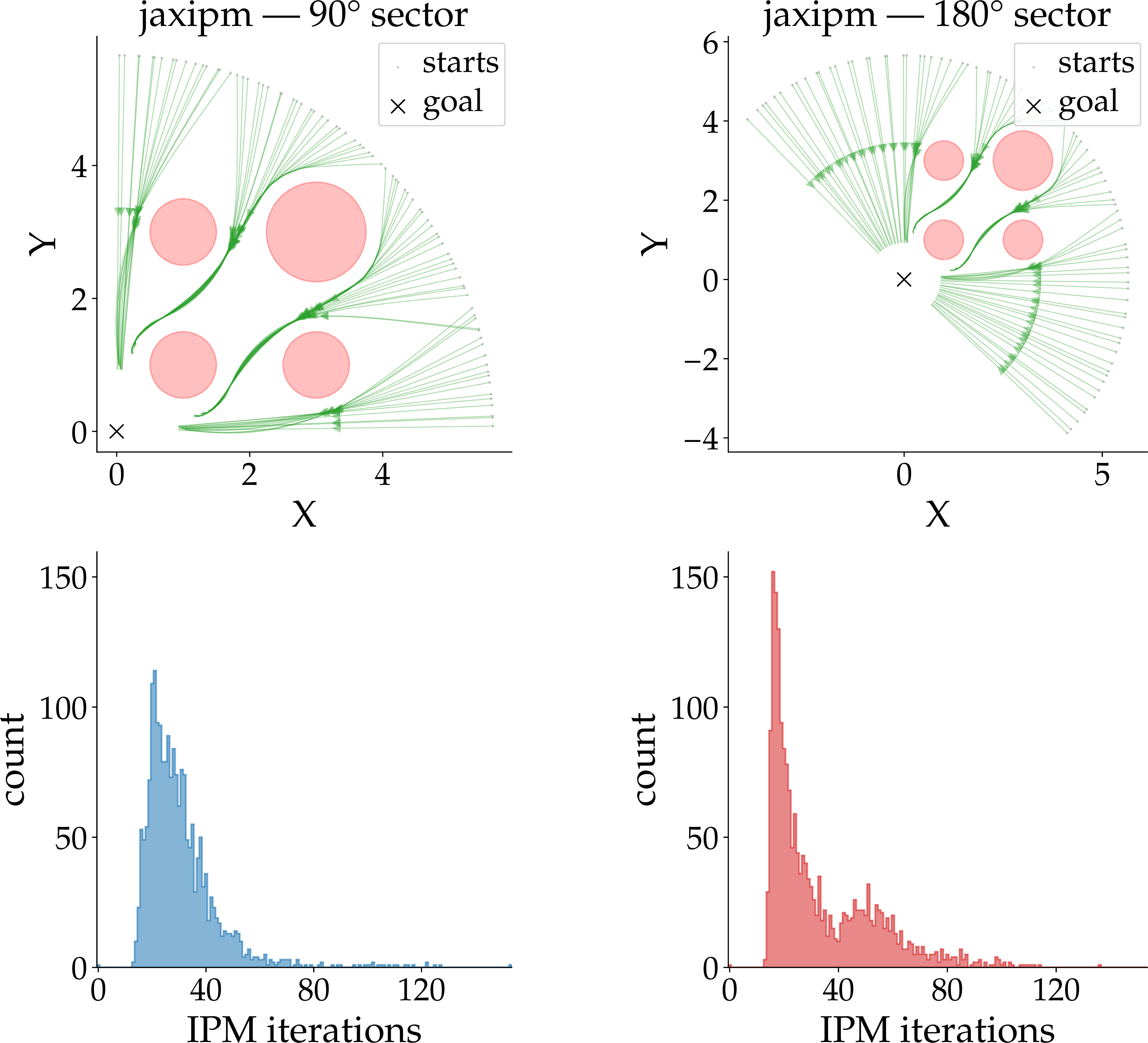
Throughput. We test throughput by setting up a batch of quadrotors that must each navigate to a common position from varying initial positions. The initial positions are a circular arc of \(90^\circ\) or \(180^\circ\) as can be seen in Figure 3. We placed the obstacles in such a way that they only interact with the trajectories in the central \(90^\circ\) section of the arc of initial positions.
We observe the \(180^\circ\) scenario has two types of optimizations, ones that interact with the obstacles, and ones that don’t, leading to two distinct peaks in the iteration count distributions, as can be seen in Figure 2. If our iteration level batching is working correctly, we expect to see similar throughput speedups over IPOPT in both the more homogeneous \(90^\circ\) and heterogeneous \(180^\circ\) scenarios, and this is exactly what we see in Table 2, where we achieved \(25.25\times\) and \(24.74\times\) throughput improvements over IPOPT, respectively.
Scalability. We test scalability in two ways: firstly, we create a test that scales difficulty, and secondly, we create a test that scales dimensionality.
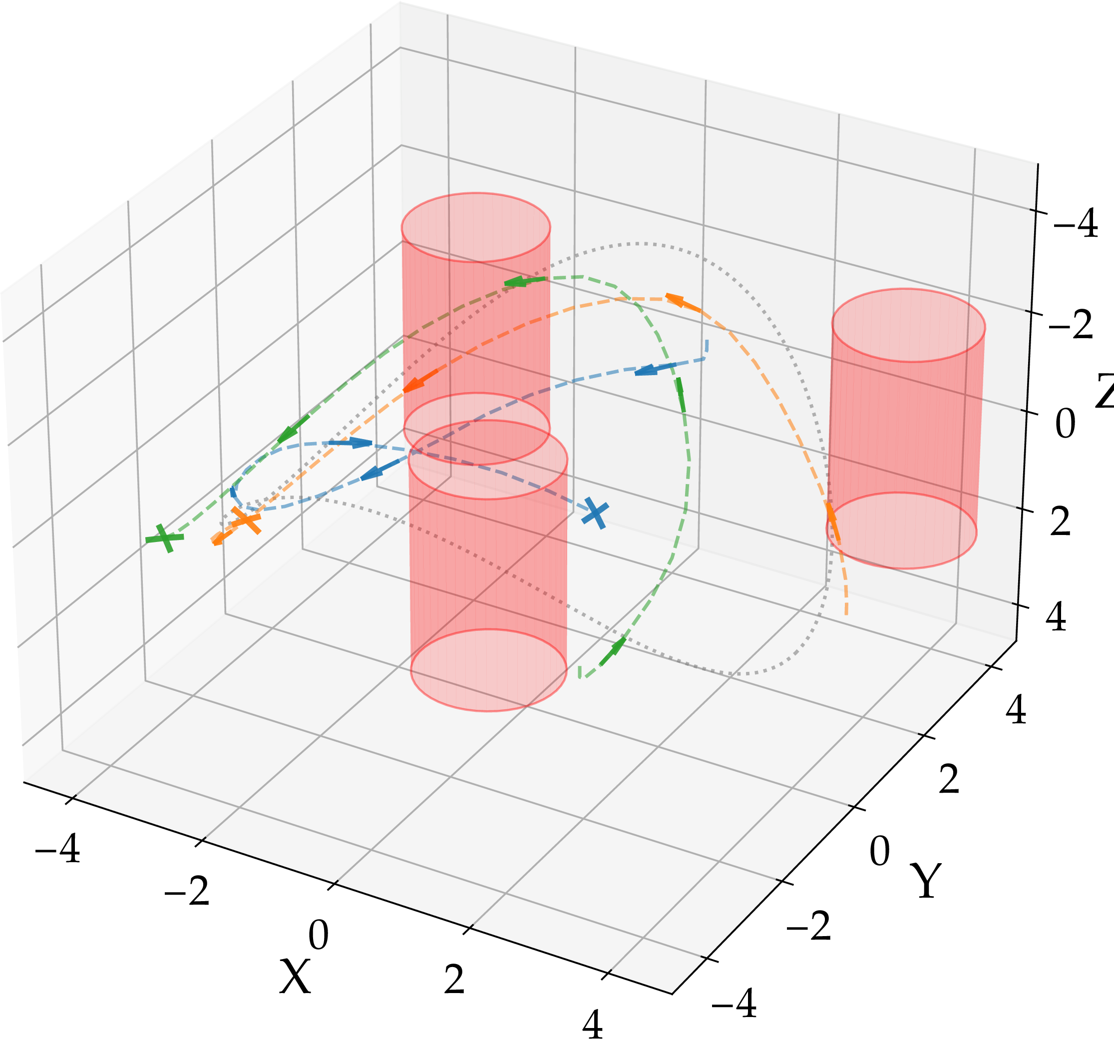
How does scaling difficulty affect jaxipm? Our first test for scaling consists of a reference tracking task whilst simultaneously avoiding time-varying obstacles, whose trajectories are known to the optimizer a priori. We increase
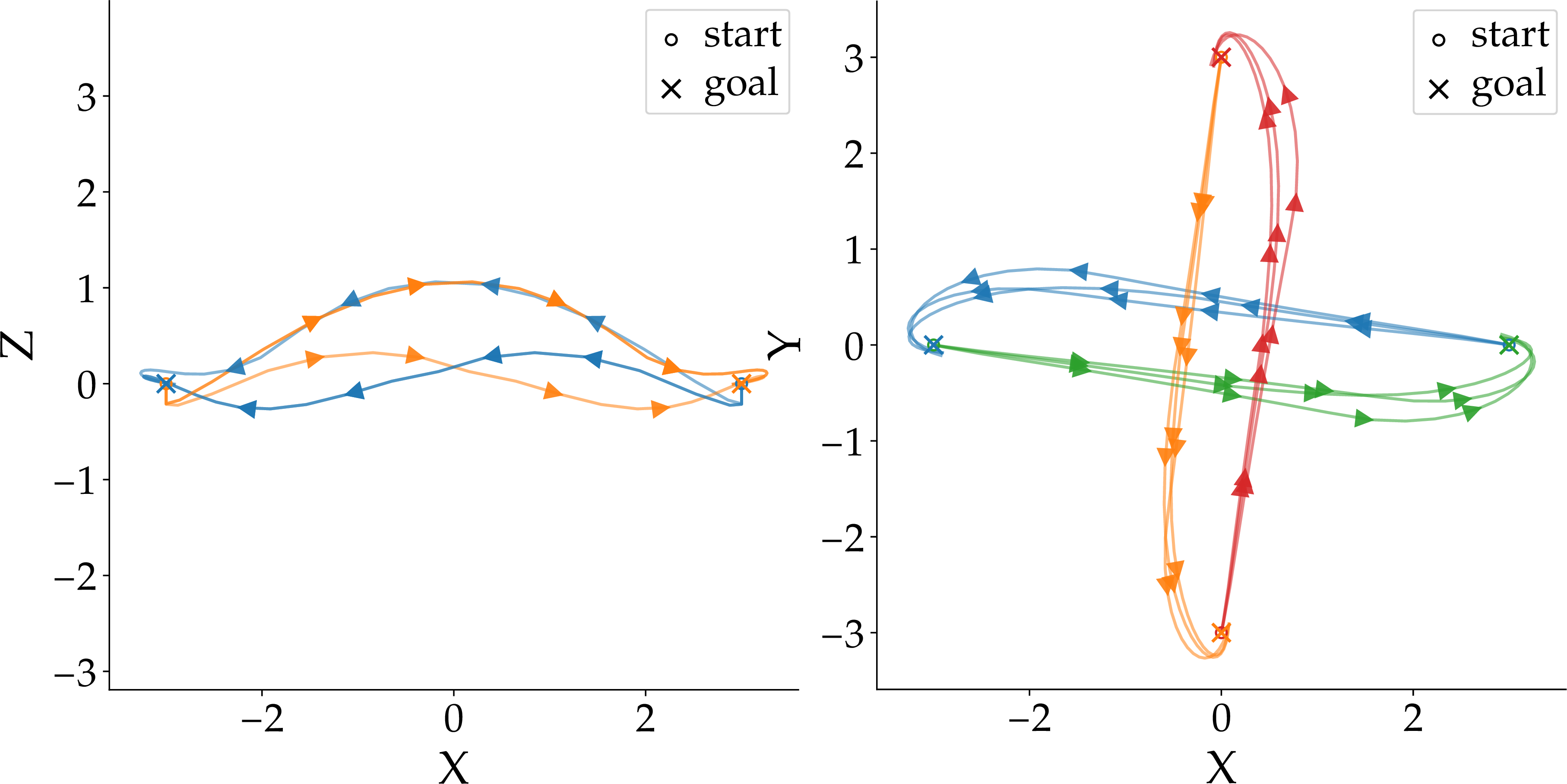
difficulty by increasing the velocity of the reference being tracked \(\bar{v}\), which is constant for each optimization. We provide each quadrotor instance with its own time-varying reference, and a visualization of a
batch of solutions can be seen in Figure 4.
We observe in Table 3 that our method always has the highest throughput, and appears to improve against baselines as difficulty increases. Empirically, this seems to be due to our method requiring a similar number of iterations at each difficulty level.
| \(\bar{v}\) (m/s) | Solver | solves/s | speedup | avg.cost | avg.iters |
|---|---|---|---|---|---|
| 1.0 | IPOPT | 3.41 | 1.00\(\times\) | 262.50 | 23.3 |
| MadNLP | 6.73 | 1.97\(\times\) | 251.94 | 30.6 | |
| jaxipm | 15.77 | 4.63\(\times\) | 252.75 | 52.1 | |
| IPOPT | 2.39 | 1.00\(\times\) | 537.44 | 28.2 | |
| MadNLP | 1.69 | 0.71\(\times\) | 537.62 | 37.5 | |
| jaxipm | 22.54 | 9.43\(\times\) | 554.22 | 45.3 | |
| 2.0 | IPOPT | 1.80 | 1.00\(\times\) | 1134.16 | 47.9 |
| MadNLP | 4.82 | 2.68\(\times\) | 1133.32 | 44.8 | |
| jaxipm | 22.10 | 12.28\(\times\) | 1146.49 | 49.8 |
How does scaling dimensionality affect jaxipm? Our second test for scaling consists of a multi-quadrotor consensus task, where multiple quadrotors are asked to switch positions whilst maintaining a minimum separation distance with
every other quadrotor throughout. We scale dimensionality by increasing the number of quadrotors in a scene from 2 to 4 as seen in Figure 5. This means that the 2 and 4 quadrotor cases have 1012 and 2024 optimization
variables, respectively, excluding slack variables from inequality constraints.
We observe that although we have at least an order of magnitude throughput advantage over IPOPT, our speedup is halved from \(32.85\times\) to \(16.03\times\) when moving from \(2\) to \(4\) quadrotors. This is because we cannot fit as many large problems in the limited GPU memory, and so we saturate the GPU with a smaller batch size. Therefore, although still over an order of magnitude faster, our speedups over IPOPT diminish with problem dimension.
| \(N_{\text{quads}}\) | Solver | solves/s | speedup | avg.cost | avg.iters |
|---|---|---|---|---|---|
| 2 | IPOPT | 0.230 | 1.00\(\times\) | 756.31 | 177.0 |
| MadNLP | 1.218 | 5.30\(\times\) | 756.31 | 150.9 | |
| jaxipm | 7.56 | 32.85\(\times\) | 756.31 | 128.4 | |
| IPOPT | 0.058 | 1.00\(\times\) | 1537.69 | 216.0 | |
| MadNLP | 0.353 | 6.05\(\times\) | 1537.70 | 279.7 | |
| jaxipm | 0.93 | 16.03\(\times\) | 1537.70 | 222.0 |
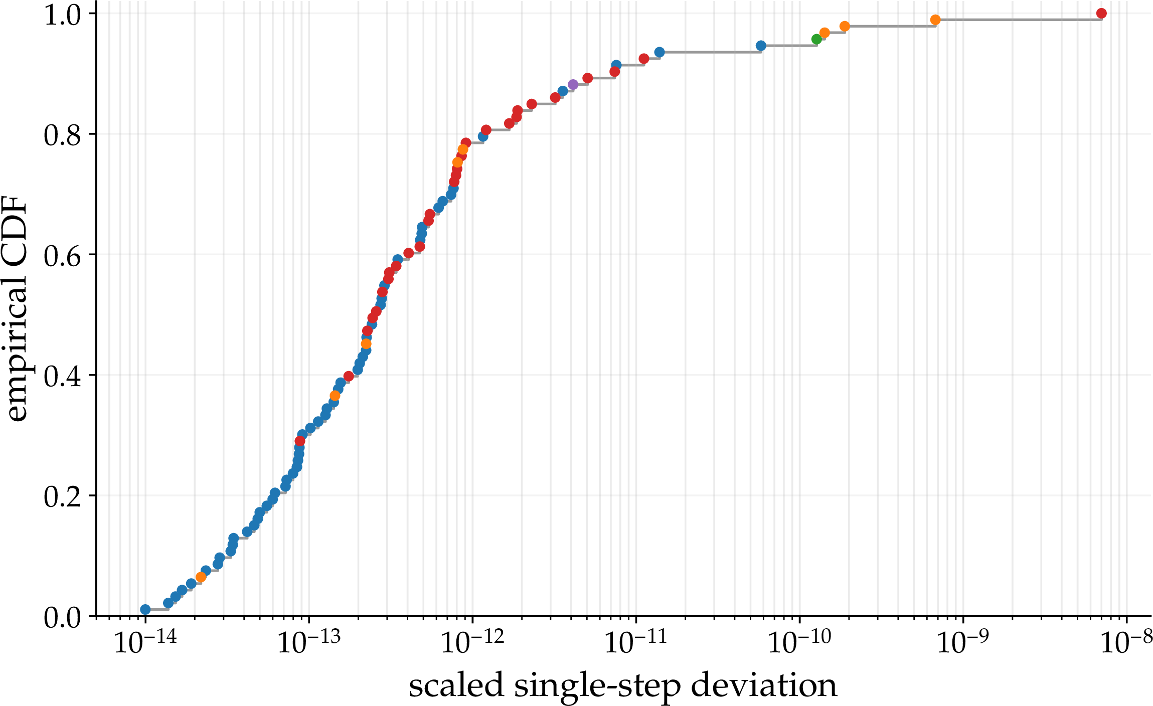
Correctness. We set up one additional test to validate our algorithmic parity with IPOPT. Here we run IPOPT to convergence from a single challenging starting point in the navigation task that we plotted in Figure 3. Specifically, we consider the (\(x=4\), \(y=4\)) starting point. Among all tests in this section, this optimization goes through the most control
flow branches of IPOPT. These include second order correction, soft/hard feasibility restoration, and free/monotone barrier update switches (see Table 1). We save the complete IPOPT state at every iteration. We then load
this complete state into jaxipm and step jaxipm once. We then convert the new jaxipm state and the next IPOPT state into vectors \(v^\texttt{jaxipm}\) and \(v^\text{IPOPT}\), respectively. We then find the largest scaled elementwise deviation \(e_v\) using the following formula (restricted to quantities IPOPT computes, fields with no IPOPT
counterpart are excluded):
\[e_v \;=\; \max_i \; \frac{\bigl\lvert v_i^{\texttt{jaxipm}} - v_i^{\text{IPOPT}} \bigr\rvert}{1 + \bigl\lvert v_i^{\text{IPOPT}} \bigr\rvert}.\]
By normalizing the deviation by \(1 + \bigl\lvert v_i^{\text{IPOPT}} \bigr\rvert\), this metric measures the relative deviation without incurring a singularity at zero7. We then report \(e_v\) for each iteration in Figure 6.
As we can see from Figure 6, all deviations fall beneath \(10^{-8}\). This tests an entire optimization directly against IPOPT, and verifies our solver’s algorithmic parity with IPOPT across
all control flow branches activated in this optimization. Beyond this test, we have evaluated the remaining untested parts of jaxipm with further unit tests. Figure 6 provides empirical evidence for
jaxipm being a feature-complete recreation of IPOPT, built from the ground up with GPU-batching in mind.
7 Conclusion↩︎
We present jaxipm, the first GPU-batched NLP optimizer, which can run thousands of independent IPOPT optimizations concurrently on a single GPU. Our two contributions that enable this are heterogeneous iteration fusion, which
collapses IPOPT’s branching recovery mechanisms into a single iteration type for all optimizations, and iteration level batching, which minimizes GPU idle time. We evaluate jaxipm’s throughput, scalability, and correctness across a
variety of NMPC quadrotor tasks and outperform IPOPT and MadNLP in terms of throughput at every problem tested.
We see several future directions for jaxipm. Imitation-learning pipelines could leverage jaxipm to build datasets of optimal trajectories at scales currently impractical on CPU. Hybrid MPPI-MPC schemes could become realizable
with the batch solution of many NLPs. GPU-based reinforcement-learning frameworks could integrate NLPs natively into their training loops.
References↩︎
\(^{1}\)J. Viljoen, M. Tomizuka, and N. Mehr are with the Department of Mechanical Engineering, University of California, Berkeley, CA, USA.
{john_viljoen, tomizuka, negar}@berkeley.edu↩︎\(^{2}\)J. Haffner was with the Department of Biosystems Science and Engineering, ETH Zürich, Switzerland, during the completion of this work.
johanna@haffner.dev↩︎This work has been submitted to the IEEE for possible publication. Copyright may be transferred without notice, after which this version may no longer be accessible.↩︎
Note that the changes necessary to handle the one-sided bounds are outlined in Section 3.4 in [7].↩︎
We are able to ignore these affine inequality constraints in the optimality conditions as we enforce them by construction throughout the optimization via the fraction to boundary rule. For more information, see Section 2.2 in [7].↩︎
The remaining steps \(\Delta z_L, \Delta z_U\) can be recovered from equations detailed in Section 2.2 in [7].↩︎
This error metric underpins
numpy.isclosewhen \(\texttt{rtol}==\texttt{atol}\).↩︎