Probing the molecular gas content of galaxies in an over-dense group at z\(\sim\)0.7: a test case for environmental quenching
June 24, 2026
To probe the impact of group environment on molecular gas reservoirs at intermediate redshift, we observed the CO(2-1) emission in the galaxy group COSMOS-Gr30 at \(z \sim 0.7\) with IRAM’s NOEMA and 30m telescopes. This dense environment, located at the intersection of large-scale cosmic web filaments, has the specificity to host a large (\(\sim 10^{4}\) kpc\(^{2}\)) ionized gas structure revealed by MUSE. We detect CO emission in four galaxies of the group at \(\mathrm{S/N} > 5\) and derive upper limits for the remaining group members with secure spectroscopic redshifts. Stacked measurements indicate that group galaxies exhibit on average molecular gas contents reduced by \(\sim 0.5\) dex relative to field scaling relations, corresponding to gas fractions that are \(20\%\) to \(40\%\) of those found in typical main-sequence galaxies. Although the uncertainties are significant, this suggests that environmental processes efficiently deplete molecular gas reservoirs in the galaxies of this group. The 30m observations place an upper limit on the molecular gas associated with the extended ionized structure, \(M_{\rm gas} < 2 \times 10^{10}\) M\(_{\sun}\), implying that less than a third of the gas in the intra-group medium is in a cold, star-forming phase. Together, these results contribute to show how environmental mechanisms in dense group environments act to remove or suppress molecular gas within galaxies, capturing quenching processes in action.
1 Introduction↩︎
The role of environment on the growth and mass assembly processes of galaxies remains a puzzle today. How do dense environments, such as groups and clusters, affect the star formation rate (SFR) ? What are the physical processes responsible for star formation quenching in these structures? Is the regulation of star formation mostly driven by internal galactic properties, such as morphology or mass, or by external, i.e. environmental, conditions, such as gas stripping or tidal interactions?
Observations have shown that star formation in galaxies mostly happened along what is called the “main sequence” (MS), an evolving and relatively tight empirical relation between the SFR and the stellar mass (\(\rm M_\star\)) of galaxies [1]–[6]. Such a robust relation, observed so far up to \(z \sim 9\) [7], promotes an overall smooth and continuous mode for star formation in galaxies. A long-lived star formation cycle could be sustained by a continuous supply of gas and/or minor mergers [8]–[12], providing large reservoirs of molecular gas to fuel star formation [13]–[19]. Typical star-forming galaxies are expected to evolve along the MS in a quasi-equilibrium between inflows, outflows, and star formation [20]–[22], until their star formation is quenched when they reach a typical stellar mass of \(\sim 10^{11}\)M\(_{\sun}\) [23]. Then, massive galaxies rapidly cease their star formation and drop below the MS to populate the “red sequence”.
Physical processes responsible for this star formation quenching are not yet fully understood. Quenching could be due to a combination of gas removal by winds or heating from supernovae and/or active galactic nuclei (AGN) [24]–[30], a decline in gas accretion if inflows cannot penetrate deep inside massive haloes [9], [31]–[37], a change in morphology [38], disk instabilities due to the presence of bars [39], and also environmental effects, such as gravitational [40] and hydrodynamical perturbations [31], [41]–[44]. Both the pristine gas accreted from the cosmic web and that recycled from the galaxies through outflows, tidal interactions or stripping are expected to result in gas reservoirs outside galaxies. The detection of such reservoirs is elusive, notably as the different gas phases, of different temperature, are mixed together and distributed on different scales [44]. But dense galactic environments could be the best targets to search for them. Indeed, large amounts of molecular gas (on the order of \(10^{10}\) M\(_{\sun}\)spread over tens of kpc) have been observed in the intra-cluster medium of nearby clusters, although it is generally associated with well-identified galaxies [45]–[49]. Similar amounts have been detected in high-\(z\) proto-clusters, such as the Spiderweb at \(z\sim 2.2\), where the majority of the molecular gas lies between the galaxies [50], [51]. These recycled gas reservoirs may sustain ongoing star formation and drive the assembly of the massive galaxies found in modern cluster cores. Similar phenomena are observed on the smaller scale of galaxy groups. In Stephan’s Quintet, molecular gas is distributed across shocked ridges, tidal tails, and intergalactic regions, forming highly turbulent, unbound giant molecular complexes [52]–[54]. Given that some of the environmental processes responsible for quenching star formation operate over several Gyr [55], [56], the recently-quenched groups observed in the local Universe [57], [58] likely initiated this transition as early as \(z > 0.5\).
![Figure 1: JWST image (F277W band, logarithmic scale, arbitrary unit) of the over-dense region in the CGr30 galaxy group at z\sim 0.7, from the COSMOS-Web program [59], with galaxy group members marked using circles. Logarithmic MUSE []contours from [60], [61] are overlaid in blue. Eight galaxies of the group, including an AGN-host (#71), are embedded in a huge []-bright structure of ionized gas extending over \sim 10^4 kpc^2. Both the NOEMA primary beam (solid black circle of 38diameter at \rm \nu_{obs} = 133.6~GHz) and the 30m beam (dashed black circle of 20diameter at the same observing frequency) cover these galaxies. Galaxies observed by MUSE are identified by their MUSE IDs and colored according to their position with respect to the main sequence (on in green, below in red and above in blue, cf. Fig. 2). Galaxies whose CO(2-1) emission was detected as part of our NOEMA program, namely #71, #105, #119, and #131, are highlighted in bold. The MUSE field of view is indicated by a light gray line.](/article/2606.26320/images/jwst_o2_noema_30m_paper_v2.png "fig:")
In this article, we report molecular gas observations with IRAM’s NOrthern Extended Millimeter Array (NOEMA) and 30m telescope of a remarkable galaxy group at \(z\sim 0.7\). This study aims to characterize star formation regulation and quenching processes in a dense environment at intermediate redshift, between the peak epoch of star formation and today. Specifically, we quantify the molecular gas reservoirs within the group galaxies, assess their depletion relative to typical main-sequence galaxies, and investigate the potential presence of diffuse molecular gas within the intra-group medium. The target group, COSMOS-Gr30 (or CGr30) has been chosen in the Muse gAlaxy Groups In Cosmos (MAGIC) survey [61] for the presence of a massive and extended structure of []\(\lambda\lambda\)3726,3729-bright ionized gas in its most over-dense region [60], as shown in Fig. 1. The present NOEMA and 30m observations provide insights into the overall molecular gas content, both in the group galaxies and in the intra-group medium, that could potentially be available for future star formation. Section 2 presents the target galaxy group and the observations; Section 3 shows the results; Section 4 discusses the results and concludes. Appendix 5 further discusses the position of the group within the cosmic web; Appendix 6 considers alternative []SFR estimates; and Appendix 7 presents the star formation history (SFH) of the group galaxies, where available. Throughout this paper, we assume a flat \(\Lambda\)CDM universe with \(\Omega_m = 0.3\), \(\Omega_\Lambda = 0.7\), and \(H_0 =70 \rm~ km s^{-1} Mpc^{-1}\).
2 Observations↩︎
2.1 COSMOS-Gr30↩︎
The group targeted in the current study, COSMOS-Gr30 (or CGr30, 10:00:35.2 +02:03:44.0 J2000), was chosen from a sample of 14 groups at intermediate redshift (\(0.3<z<0.8\)) within the COSMOS field [62] drawn from the zCOSMOS 20k group catalog [63] that were observed with the Multi Unit Spectroscopic Explorer [64] as part of the Muse gAlaxy Groups In Cosmos (MAGIC) survey [61]. This survey was designed to explore the impact of environment on galaxy evolution over the last 8 billion years, covering a wide range of environments from relative isolation to dense groups and clusters. CGr30 is the group that locally shows the highest overdensity of the sample, with 44 galaxies unambiguously spectroscopically identified with redshifts between \(0.719 \leq z \leq 0.732\) in the 1 arcmin\(^2\) MUSE FoV with a velocity dispersion of \(\sim 400\) km s\(^{-1}\). This relatively high group velocity dispersion makes this group particularly suited to study environmental quenching, since its galaxies are expected to experience environmental processes over a few Gyr before merging. Most importantly, the deep MUSE observations revealed a large and massive structure of []\(\lambda\lambda\)3726,3729-bright ionized gas, extending over \(\sim 10^4\) kpc\(^2\) and weighting \(\sim 5 \pm 3\times 10^{10}\) M\(_{\sun}\)[60]. Eight of the group galaxies (\(\sim\) 1/5 of the members) are part of this over-density and are embedded in the gaseous structure (see Fig. 1) and seem to constitute a sub-group with a velocity dispersion of about 200 km s\(^{-1}\). The []-emitting diffuse gas is not uniform and displays some filaments and more concentrated regions, although not necessarily centered on the galaxies involved in the structure. This suggests that it was extracted from galaxies through tidal forces, outflows due to star formation and AGN activity, and possibly ram-pressure stripping due to previously-stripped material or more pristine gas from the cosmic web. Indeed, CGr30 is located in a larger scale structure that is identified as the COSMOS-Wall [65], at an intersection between cosmic web filaments, as shown in Appendix 5. Nevertheless, the galaxies of the group do not show clear morphological signs of interactions [60]. As described in [60], []kinematics separate two main regions in the extended gas structure (Northern-East vs Southern-West in Fig. 1). The velocity offset between the two is larger than \(\sim 200\rm ~km/s\), and each region seems to be kinematically linked with a massive galaxy, respectively #98 and #71 (\(\rm M_{\rm star}\approx 10^{10.5-11}\)M\(_{\sun}\)). Among these two galaxies, we note that #71 is an active galactic nucleus (AGN) host, as shown by broad emission lines in the nucleus, a bright [] line with respect to []and \(\rm H{\beta}\), [] and [] lines, and X-ray emission [60]. The other galaxies are star-forming and less massive (\(\rm M_{\rm star} \approx 10^{9-10.5}\)M\(_{\sun}\)).
Since the surveyed group lies in the COSMOS field, it benefits from ancillary data which enable to infer different galaxy physical properties. We use the stellar masses, SFRs, and extinctions derived in [61] from spectral energy distribution (SED) models. Those models were constrained with the Code Investigating GALaxy Emission [66] from the MUSE spectroscopic redshifts and from the COSMOS2020 photometric measurements in 3diameter apertures in 32 bands, from UV to radio centimeter [67]. As explained in more details in [61], single stellar populations of [68] were used with a [69] initial mass function and a fixed
metallicity of 0.02 dex. The SFH is a delayed exponential law with flexibility in the most recent period of the SFH as described in [70], [71]. The attenuation law is a modified [72] law with a fixed total to selective extinction
ratio \(R_V = 3.1\), and the dust template model used is that of [73]. We compared the resulting stellar masses with
values obtained using Fast [74] with a synthetic library generated from the stellar population synthesis models of [75], a [76] initial mass function, an
exponentially declining SFR, and a [72] extinction law as in [77], and found good agreement. As is common for SED-based SFR estimates [78], [79], the values from [61] involve significant uncertainties which we account for in our analysis. In order to be
consistent between MUSE and NOEMA data, we also convolved the MUSE datacube to the spatial resolution of NOEMA, assuming an elliptical Gaussian beam and extracted both NOEMA and MUSE spectra at the same sky positions. We used pPXF [80]–[82] to determine the line-of-sight velocity of the stars
using the E-MILES stellar population synthesis templates [83] and to remove the continuum contribution from the spectra, following the same
strategy as in [60]. We used multiplicative polynomials of order 10 to fit the continuum. Such polynomials are well suited to remove the continuum with
a reduced impact on the shape of emission lines. We checked that they provide similar line-of-sight velocities as when using additive polynomials, within less than \(\pm14\) km s\(^{-1}\).
We also note that whereas the spectral resolution of the E-MILES templates is larger than that of MUSE at the redshift of CGr30, this does not prevent us from getting accurate fits as long as the observed velocity dispersion of the integrated spectra
remains larger than the template resolution, which corresponds to about \(\sim 50\) km s\(^{-1}\), which is the case in practice for all galaxies, except for #57, #93, and #123, although a
visual inspection of the continuum-subtracted spectra suggests that the fit is correct. We then fitted for each MUSE continuum-subtracted spectrum the []doublet using the 1D function of the Camel code1 to infer velocities with respect to the systemic redshift of the group \(z=0.7251\), as well as the doublet velocity dispersion. To infer the offset from the MS, we adopt the
\({\rm SFR}(MS;z,M_\star)\) parametrization derived by [77] for the MAGIC sample, applying a downward adjustment of
0.12 dex to account for the average offset between their []SFRs and the SED SFRs of [61]2. Table 1 lists some of the properties of the 17 CGr30 galaxies falling within the NOEMA primary beam. Four of these galaxies (#57, #61, #93, #123) were not detected in []with MUSE,
while the two lowest-mass galaxies (#69, #78) do not yield secure pPXF fits.
| \({\rm ID}\) | RA | DEC | \(z\) | \(\log M_\star\) | \(\log{\rm SFR}\) | \(\varv_{\rm pPXF}\) | \(\varv_{\rm \oii}\) | \({\rm FWHM_{\rm \oii}}\) | \(\delta{\rm MS}\) | \(\log M_{\rm exp}\) |
| \(\rm[M_\odot]\) | \(\rm[M_\odot{\rm yr}^{-1}]\) | \([{\rm km\;s^{-1}}]\) | \([{\rm km\;s^{-1}}]\) | \([{\rm km\;s^{-1}}]\) | \(\rm[M_\odot]\) | |||||
| 49 | 10:00:34.2648 | +02:03:39.456 | \(0.7244\) | \(9.42 \pm 0.06\) | \(-0.02\pm 0.86\) | \(-24\) | \(-123\) | \(124\) | \(0.14\) | \(9.51\) |
| 57 | 10:00:34.5144 | +02:03:44.676 | \(0.7251\) | \(9.18 \pm 0.03\) | \(-2.90\pm 2.01\) | \(-126\) | \(-2.56\) | \(7.99\) | ||
| 59 | 10:00:35.1888 | +02:03:43.236 | \(0.7231\) | \(9.19 \pm 0.06\) | \(0.97\pm 0.32\) | \(-316\) | \(-335\) | \(163\) | \(1.31\) | \(9.96\) |
| 61 | 10:00:35.4648 | +02:03:38.160 | \(0.7239\) | \(10.06 \pm 0.11\) | \(1.09\pm 0.27\) | \(-196\) | \(0.79\) | \(10.22\) | ||
| 68 | 10:00:35.1264 | +02:03:40.752 | \(0.7260\) | \(10.28 \pm 0.08\) | \(-0.37\pm 2.67\) | \(124\) | \(-283\) | \(279\) | \(-0.83\) | \(9.52\) |
| 69 | 10:00:34.4856 | +02:03:48.888 | \(0.7255\) | \(8.30 \pm 0.19\) | \(-0.30\pm 1.91\) | \(82\) | \(79\) | \(0.67\) | \(9.12\) | |
| 71 | 10:00:35.7120 | +02:03:38.016 | \(0.7249\) | \(10.94 \pm 0.05\) | \(2.15\pm 0.47\) | \(-46\) | \(-34\) | \(436\) | \(1.22\) | \(10.95\) |
| 78 | 10:00:33.8856 | +02:03:51.588 | \(0.7271\) | \(8.12 \pm 0.11\) | \(-1.38\pm 2.03\) | \(302\) | \(92\) | \(-0.29\) | \(8.53\) | |
| 82 | 10:00:35.5560 | +02:03:45.432 | \(0.7268\) | \(10.10 \pm 0.04\) | \(0.42\pm 0.46\) | \(279\) | \(279\) | \(393\) | \(0.09\) | \(9.89\) |
| 93 | 10:00:34.1016 | +02:03:53.028 | \(0.7250\) | \(9.70 \pm 0.02\) | \(-3.42\pm 4.11\) | \(-105\) | \(-3.46\) | \(7.84\) | ||
| 98 | 10:00:35.1720 | +02:03:46.764 | \(0.7250\) | \(11.09 \pm 0.08\) | \(0.14\pm 0.28\) | \(-115\) | \(-42\) | \(535\) | \(-0.90\) | \(9.96\) |
| 105 | 10:00:34.4616 | +02:03:53.064 | \(0.7269\) | \(10.46 \pm 0.06\) | \(-0.37\pm 1.28\) | \(319\) | \(319\) | \(280\) | \(-0.95\) | \(9.56\) |
| 110 | 10:00:34.8816 | +02:03:54.216 | \(0.7267\) | \(10.06 \pm 0.10\) | \(-0.24\pm 0.75\) | \(317\) | \(309\) | \(97\) | \(-0.54\) | \(9.54\) |
| 114 | 10:00:34.0512 | +02:03:55.944 | \(0.7242\) | \(9.61 \pm 0.17\) | \(-0.09\pm 0.81\) | \(-106\) | \(-110\) | \(171\) | \(-0.06\) | \(9.52\) |
| 119 | 10:00:35.3544 | +02:03:52.200 | \(0.7247\) | \(10.60 \pm 0.07\) | \(0.06\pm 2.02\) | \(-153\) | \(-173\) | \(141\) | \(-0.63\) | \(9.81\) |
| 123 | 10:00:34.9128 | +02:04:00.372 | \(0.7234\) | \(9.74 \pm 0.07\) | \(-2.00\pm 1.59\) | \(-393\) | \(-2.07\) | \(8.57\) | ||
| 131 | 10:00:35.0832 | +02:03:50.652 | \(0.7230\) | \(10.73 \pm 0.12\) | \(0.66\pm 0.76\) | \(-405\) | \(-253\) | \(622\) | \(-0.12\) | \(10.15\) |
![Figure 2: Position of the 17 galaxies of COSMOS-Gr30 within the NOEMA primary beam with respect to the MS, where the offset from the MS (\delta{\rm MS} = {\rm SFR/SFR}({\rm MS};z,M_\star)) is plotted as a function of the stellar mass (M_\star) and the reference {\rm SFR}({\rm MS};z,M_\star) is that of [77], with a downward adjustment of 0.12 dex. The solid, dashed, and dotted horizontal lines are respectively the MS ridge, its 0.3 dex scatter, and \pm 1 dex from it. Galaxies whose CO(2-1) emission was detected are indicated with crosses. Error bars correspond to the uncertainties in M_\star and SFR.](/article/2606.26320/images/targets_MS.png "fig:")
2.2 NOEMA observations↩︎
To probe the molecular gas content of CGr30 galaxies at \(z\sim0.725\), we targeted the \(^{12}\)CO(2-1) carbon monoxide emission line (\(\rm \nu_{rest} =
230.538~GHz\)) falling in NOEMA’s 2mm band. This line allows direct comparison with other molecular gas surveys such as PHIBSS2 [19] and
it is the lowest-J CO line available with NOEMA at the galaxies’ redshifts. Since the targets are all separated by at least 2, the observations were carried out in configuration C to achieve a spatial resolution of \(\sim\)1.9that does not resolve individual galaxies. The NOEMA primary beam of 38encompasses 17 group members with secure redshifts, stellar masses and SFRs. Some of their properties are listed in Table 1, and their location with respect to the MS is shown in the stellar mass - SFR plane in Fig. 2. The observations were carried out at the NOEMA interferometer at the Plateau de Bure in France
between January and March 2020 with 10 antennae as part of the observational program S19BV (PI: Contini, contact: Freundlich), for a total on-source observing time of 12.2 hours. The weather conditions varied, with system temperatures ranging between 100
and 300 K depending on atmospheric conditions, wind speeds below \(20 ~\rm m\;s^{-1}\), and precipitable water vapour between 2 and 6 mm. The absolute flux scale was derived from secondary flux calibrators (3C84, LKHA101,
J1028-0236, 1038+064, 3C279, 1055+018, MWC349, 0851+202, 0906+015, J0948+003), whose fluxes are regularly measured using Jupiter satellites or planets. The data were calibrated using the clic software of the IRAM gildas package,
and further analysed and mapped using the gildas mapping and class softwares. The resulting beam size is \(2.6\times1.1~\rm arcsec^2\) and the RMS noise \(\sigma_{\rm
RMS}=0.26~\rm mJy\) over velocity channels of width \(\Delta v = 44.86~\rm km s^{-1}\), obtained using gildas mapping go noise tool.
| \({\rm ID}\) | \(F({\rm CO})\) | \(dF({\rm CO})\) | \(\rm FWHM_{\rm CO}\) | \(d\rm FWHM_{\rm CO}\) | \(\varv_{\rm CO}\) | \(d \varv_{\rm CO}\) | \(\log L_{\rm CO(2-1)}\) | \(\log M_{\rm gas}\) | \(\log \mu_{\rm gas}\) | \(\log t_{\rm depl}\) |
| \([\rm Jy~km~s^{-1}]\) | \([\rm Jy~km~s^{-1}]\) | \([\rm km~s^{-1}]\) | \([\rm km ~s^{-1}]\) | \([\rm km ~s^{-1}]\) | \([\rm km ~s^{-1}]\) | \([\rm K ~km ~s^{-1} ~pc^2]\) | \(\rm[M_\odot]\) | [Gyr] | ||
| 49 | \(< 0.06\) | \(<8.61\) | \(<9.58\) | \(<0.15\) | \(<0.60\) | |||||
| 57 | \(< 0.06\) | \(<8.60\) | \(<9.65\) | \(<0.47\) | \(<3.55\) | |||||
| 59 | \(< 0.07\) | \(<8.67\) | \(<9.72\) | \(<0.53\) | \(<-0.25\) | |||||
| 61 | \(< 0.06\) | \(<8.60\) | \(<9.41\) | \(<-0.65\) | \(<-0.68\) | |||||
| 68 | \(< 0.09\) | \(<8.79\) | \(<9.56\) | \(<-0.73\) | \(<0.93\) | |||||
| 69 | \(< 0.05\) | \(<8.51\) | \(<10.08\) | \(<1.78\) | \(<1.38\) | |||||
| 71 | \(0.43\) | \(0.05\) | 566 | 73 | \(-46\) | 36 | \(9.47\) | \(10.17\) | \(-0.77\) | \(-0.97\) |
| 78 | \(< 0.05\) | \(<8.55\) | \(<10.29\) | \(<2.16\) | \(<2.67\) | |||||
| 82 | \(< 0.10\) | \(<8.86\) | \(<9.66\) | \(<-0.44\) | \(<0.25\) | |||||
| 93 | \(< 0.06\) | \(<8.60\) | \(<9.49\) | \(<-0.22\) | \(<3.91\) | |||||
| 98 | \(< 0.12\) | \(<8.93\) | \(<9.62\) | \(<-1.47\) | \(<0.48\) | |||||
| 105 | \(0.21\) | \(0.04\) | 233 | 46 | 312 | 21 | \(9.18\) | \(9.92\) | \(-0.53\) | \(1.29\) |
| 110 | \(< 0.05\) | \(<8.56\) | \(<9.37\) | \(<-0.70\) | \(<0.61\) | |||||
| 114 | \(< 0.07\) | \(<8.68\) | \(<9.59\) | \(<-0.01\) | \(<0.68\) | |||||
| 119 | \(0.19\) | \(0.03\) | 173 | 34 | \(-140\) | 18 | \(9.13\) | \(9.86\) | \(-0.74\) | \(0.80\) |
| 123 | \(< 0.06\) | \(<8.60\) | \(<9.47\) | \(<-0.26\) | \(<2.48\) | |||||
| 131 | \(0.48\) | \(0.06\) | 579 | 79 | \(-412\) | 39 | \(9.53\) | \(10.24\) | \(-0.49\) | \(0.58\) |
2.3 30m observations↩︎
In complement to the NOEMA observations, we also observed the CO(2-1) line with the IRAM 30m telescope at Pico Veleta in Spain in order to constrain the total molecular gas content, both in the galaxies and in the intra-group medium. Any excess emission
compared to the total galaxy flux measured from the NOEMA observations could indeed reveal the molecular gas outside of the galaxies and thus help test star formation regulation models in galaxies. These observations were first carried out as part of
project 110-19 directly complementing the NOEMA project S19BV between 30 and 31 July 2020, and then as part of a dedicated project 173-20 (PI: Contini, contact: Freundlich) between 7 and 19 April 2021. The two endeavours resulted in a total on-source
observing time of 9.5 hours. As shown in Fig. 1, the 20beam of the 30m telescope at the targetted wavelength covers the []-emitting diffuse gas structure and the eight galaxies embedded in this structure. Other galaxies
(#57, #69, #105 and #110) lie at the edge of the beam. We used band E150 of the Eight Mixer Receiver (EMIR) to observe the CO(2-1) line, wobbler-switching, and both the Wideband Line Multiple Autocorrelator (WILMA) and the Fast Fourier Transform
Spectrometers (FTS) as backends. The observations were carried out in average weather conditions, with system temperatures \(\rm T_{sys}\sim 150~K\). Data reduction and analysis were performed using the class
software of the gildas package. The resulting RMS noise was \(1.7 ~\rm mJy\) over velocity channels of width \(89.74~\rm km~s^{-1}\) with WILMA, after converting the antenna
temperature into a main beam temperature using a main beam efficiency \(B_{\rm eff}=0.62\) and a point source sensitivity of \(5\rm ~Jy/K\) given the observing frequency (\(\nu_{\rm obs} = 133.6~\rm GHz\))3.
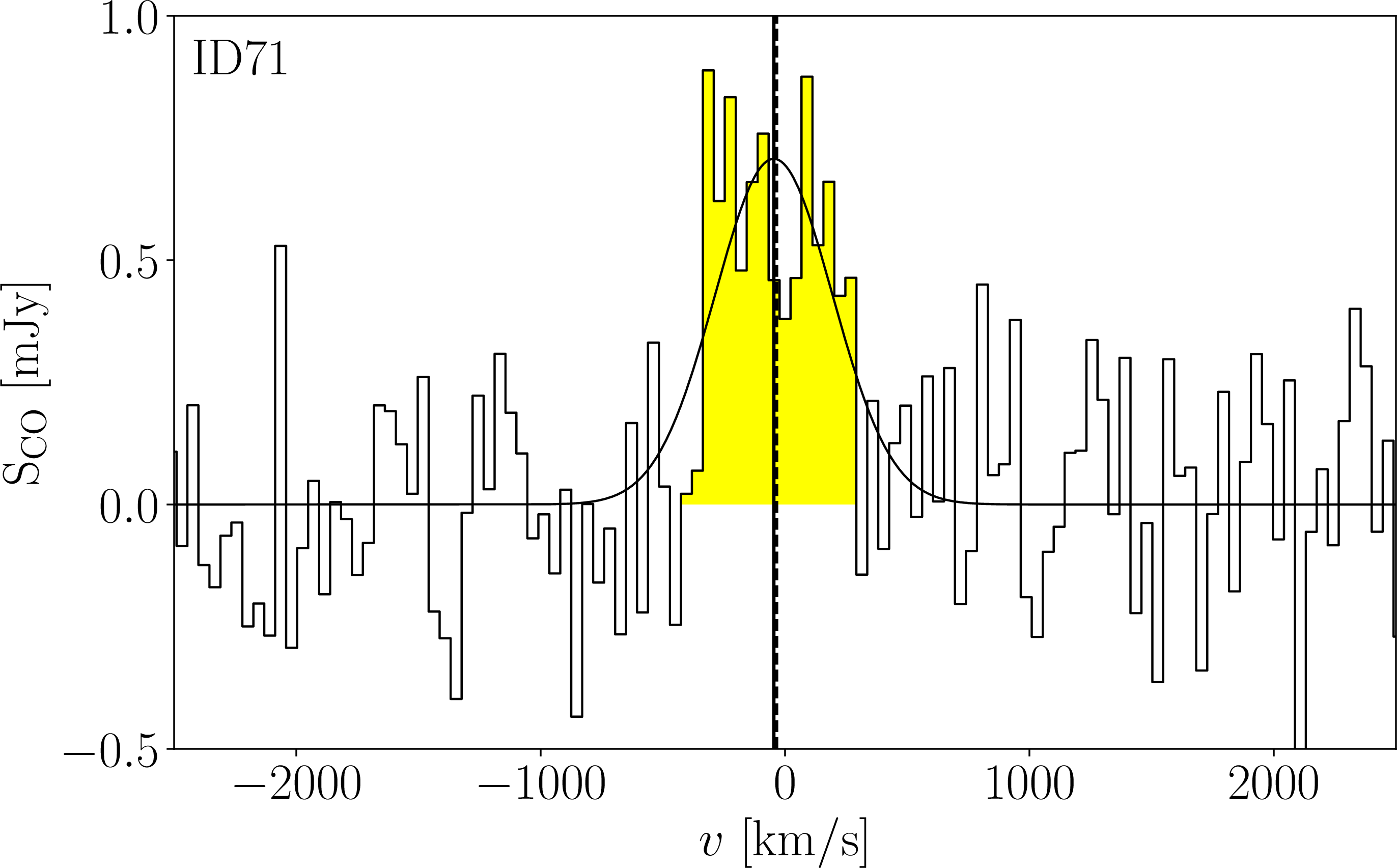
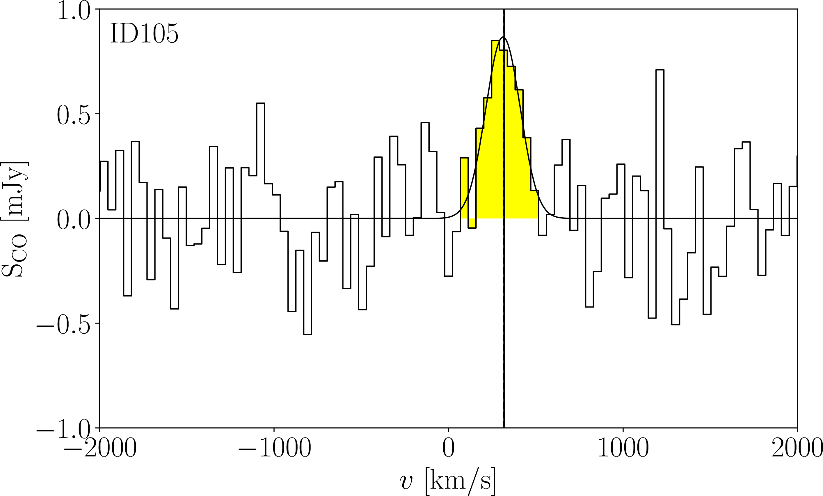
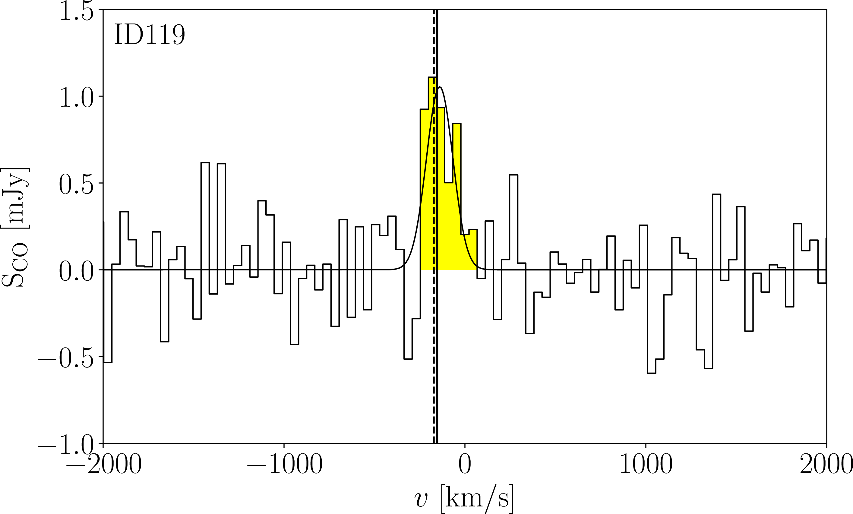
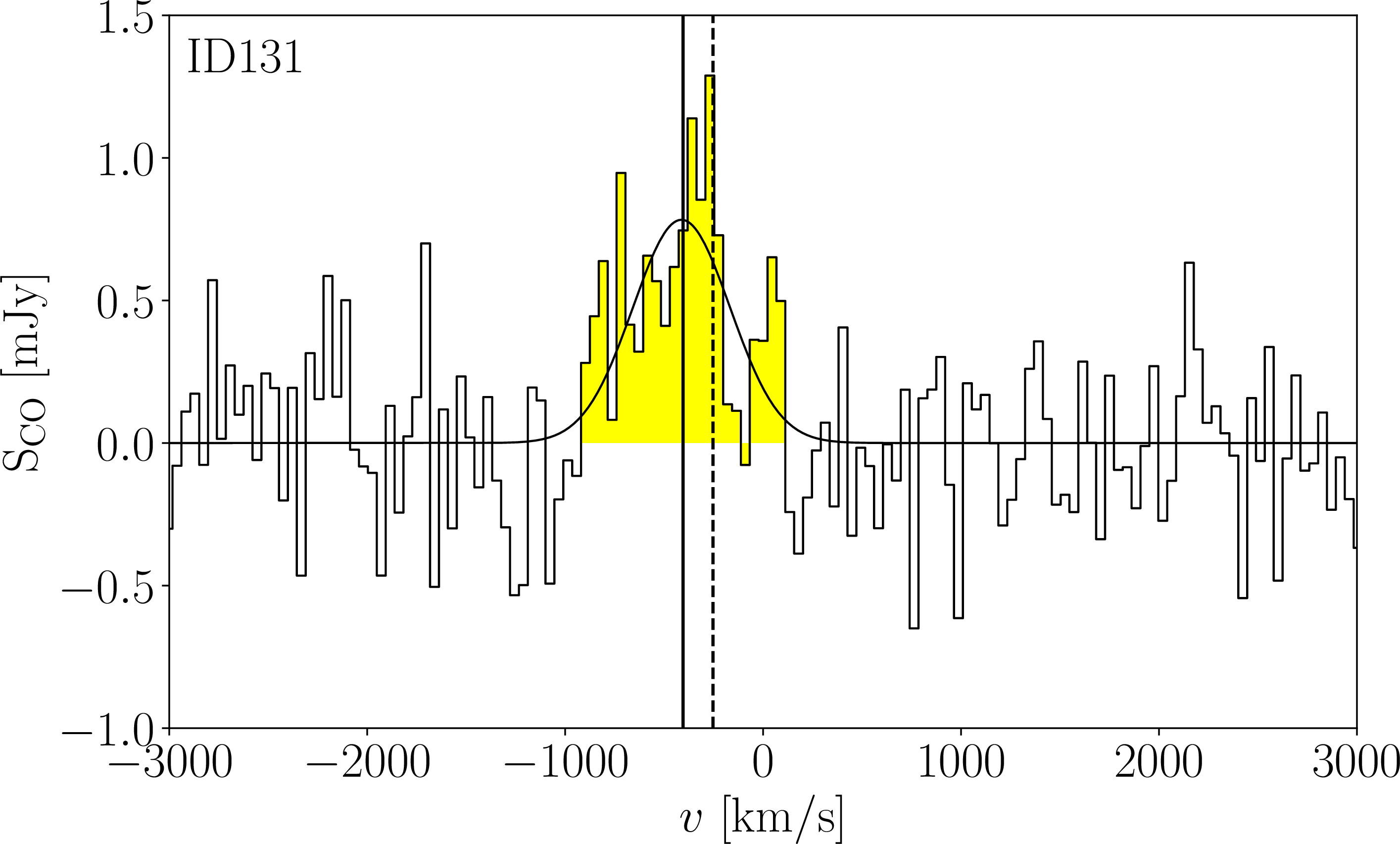
Figure 3: NOEMA CO(2-1) spectra of the four detected galaxies in the group CGr30, namely #71, #105, #119, and #131. The S/N are respectively 8.7, 5.4, 8.6, and 8.3 (cf. Table 2). The velocities \(v\) are defined with respect to the average group velocity. The velocities of the stars are shown as vertical solid lines, those of the []doublet as vertical dashed lines..
3 Results↩︎
3.1 Detections and upper limits↩︎
For each galaxy of the group, we extracted the NOEMA spectrum at the optical position by fitting the point spread function (PSF) in the \(uv\) Fourier space using gildas mapping go uvfit tool. Fitting the
unresolved sources through their \(uv\) visibilities indeed avoids the imaging and deconvolution steps, which involve assumptions to compensate for the sparse \(uv\) coverage. Table 2 summarizes the quantities derived from these galaxy spectra.
We detected the CO(2-1) line with signal-to-noise ratios \(\rm S/N>5\) for four galaxies, namely #71, #105, #119, and #131, whose spectra are displayed in Fig. 3. We perform Gaussian
fits using class, yielding the corresponding integrated line flux \(F({\rm CO})\), velocity \(\varv_{\rm CO}\) with respect to the mean group velocity, and full width at half
maximum \(\rm FWHM_{\rm CO}\). Fluxes are rescaled to take into account the NOEMA primary beam power, assuming a Gaussian beam with a 38half-power beam width. For the four detected galaxies, the S/N are respectively 8.7,
5.4, 8.6, and 8.3. As shown in Fig. 3, the velocity of the CO line closely matches that of the stars (\(\varv_{\rm pPXF}\) in Table 1) and that of the
[]emission (\(\varv_{\rm [\ion{O}{ii}]}\)), although there is a \(\sim -160\) km s\(^{-1}\)offset with the latter in the case of #131. The agreement with
\(\varv_{\rm pPXF}\) fits well with the idea that the molecular gas lies in the galaxy close to the stars, while the global offset between molecular and ionized gas velocity profiles in the case of #131 could indicate that
some of the []emission traces ionized gas being decelerated by ram pressure stripping [86]. Supporting this, [60] report a higher velocity dispersion in the diffuse []component around #131, and that the kinematics of this galaxy is different from its surrounding []gas. The agreement
between molecular and ionized gas velocity profile widths for the four galaxies also suggests that the CO and []emissions have similar extents within these galaxies. [87] derived star formation histories for some of the galaxies of CGr30, and we note that the four galaxies we detected harbor a recent star formation episode, as shown in Appendix 7,
possibly due to an influx of gas triggered by the environment. Indeed, the last star formation episode for these four galaxies took place 1 or 2 Gyr ago, hence about a group dynamical time (\(\sim\) \(1.6\rm ~Gyr\)).
![Figure 4: Stacked NOEMA CO(2-1) spectra over all galaxies in the primary beam (upper panel), over all galaxies except #71 (middle panel), and over the non-detections (lower panel). Velocities \Delta \varv are taken with respect to the stellar velocities (the []velocities for #69 and #78), and scaled to the []FWHM (to a fixed 118~\rm km s^{-1} for #57, #61, #93, #123 in the absence of []detections); fluxes are weighted by the NOEMA beam power before being stacked. The corresponding signals yield 0.89\;\rm Jy\;km\;s^{-1} with a \rm S/N = 4.7 for all galaxies, 0.63\;\rm Jy\;km\;s^{-1} with a \rm S/N = 3.9 for all galaxies without #71, and a 3\sigma upper limit 0.40 \;\rm Jy\;km\;s^{-1} for the non-detections.](/article/2606.26320/_pdflatex/ufyxdcvp.png "fig:")
For galaxies whose CO(2-1) line is undetected, we used the MUSE []FWHM to evaluate upper limits for the integrated line flux. Indeed, since the targeted galaxies are typical main sequence star-forming galaxies, obscuration is not extreme and both []and CO should trace similar star-forming regions and velocity fields. Observational studies have shown that []and CO line widths were comparable [88], [89], and this is the case for the four detected galaxies here (cf. Tables 1 and 2). We evaluated the noise within the FWHM, \(\sigma_{\rm FWHM} = \sigma_{\rm RMS} \sqrt{{\rm FWHM}\times \Delta \varv}\), with \(\Delta \varv\) the width of the velocity channels, and defined \(3\sigma\) integrated line flux upper limits as \(F_{\rm upper}= 3\times \sigma_{\rm FWHM}\), which correspond to fluxes that should have been detected at \(\rm S/N>3\) with a 50% probability [90]. For the four galaxies undetected in [](#57, #61, #93, #123), we use a fixed FWHM equal to \(118~\rm km s^{-1}\), which corresponds to the median []dispersion for galaxies with \(\log (M_\star/{\rm M_\odot}) <10\). We recall that the beam size is \(2.6\times 1.1~\rm arcsec^2\) and the experimental RMS noise \(\sigma_{\rm RMS}= 0.26 ~\rm mJy\) per \(\Delta \varv= 44.86~\rm km s^{-1}\) wide channel. Upper limit fluxes are also rescaled by the beam power.
To assess the total and average molecular gas masses in the galaxies, we further stacked the CO spectra at the optical positions of the galaxies in the NOEMA beam, shifting them by the stellar velocity, normalizing the velocities by the MUSE []FWHM, and
weighting by the NOEMA beam power. For the four galaxies undetected in [], we again use a fixed FWHM equal to \(118~\rm km s^{-1}\) instead of the []FWHM, while for the two lowest-mass galaxies without pPXF
fits we use the []velocity instead of the stellar velocity. The resulting stacked spectra for all the galaxies, for all galaxies except #71, and for the non-detected subsamble are shown in Fig. 4. We singled out #71 in the
analysis because it is an AGN, which could contaminate the estimated SFR and hence the offset from the MS as well as the molecular gas mass we can expect to measure. For all galaxies in the NOEMA beam, we obtained a signal of \(0.89 \pm 0.19~ \rm Jy~km~s^{-1}\) with an \(\rm S/N = 4.7\); for all those galaxies except #71, we obtained \(0.63 \pm 0.16~ \rm Jy~km~s^{-1}\) with an \(\rm S/N = 3.9\); for the non-detections we obtained no stacked detection but derived a 3\(\sigma\) upper limit of \(0.40 ~\rm Jy~km~s^{-1}\) from the RMS noise
(\(1.55~\rm mJy\) in channels of 0.21 times the FWHM in the bottom panel of Fig. 4). We stress that this is done without any free parameter since both the central velocities and the line widths
are constrained. The relative uncertainty on the stacked CO line fluxes are \(\rm 1/(S/N) = 21\%\) for all galaxies and \(26\%\) without #71. Finally, we searched for dust continuum
detection using the full bandwidth of the NOEMA observations, without success.
3.2 Galaxy molecular gas masses↩︎
From the integrated line fluxes or their upper limits, we derived intrinsic CO(2-1) luminosities \[\label{eq:luminosity} \left(\frac{L^\prime_{{\rm CO(2-1)}}}{\mathrm{K~km~s}^{-1}\mathrm{~pc}^2}\right) = \frac{3.25 \times 10^7}{1+z} \left(\frac{F_{{\rm CO(2-1)}}}{\mathrm{Jy~km~s}^{-1}}\right) \left(\frac{\nu_{\rm rest}}{\mathrm{GHz}}\right)^{-2} \left(\frac{D_\mathrm{L}}{\mathrm{Mpc}}\right)^2,\tag{1}\] where \(\nu_{\rm rest}\) is the rest-frame frequency, and \(D_{\rm L}\) the luminosity distance [91], and molecular gas masses \[M_{\rm gas} = \alpha_{\rm CO} L_{{\rm CO}(2-1)}^\prime / r_{\rm 21},\] where \(\alpha_{\rm CO}\) is the CO(1-0) luminosity-to-molecular-gas-mass conversion factor and \(r_{21}=L_{{\rm CO}(2-1)}^\prime/L_{\rm CO(1-0)}^\prime\) the corresponding line ratio. Following the PHIBSS2 methodology [16], [18], [19] in order to allow comparison with their results, we took the conversion factor as the geometric mean of the recipes by [92] and [93], which include a metallicity dependence, namely \[\alpha_{\rm CO} = \alpha_G \sqrt{0.67 \times \exp(0.36 \times 10^{8.67-\log{Z}}) \times 10^{-1.27\times (\log{Z}-8.67)}} ,\] where \(\alpha_G = 4.36 \pm 0.9 \rm~ M_\odot/(K~km~s^{-1} pc^{2})\) is the Galactic conversion factor and \(\log{Z} = 12+\log({\rm O/H})\) the metallicity on the [94] scale estimated from the mass–metallicity relation, \(\log{Z} = 8.74 - 0.087 \times (\log({M_{\star}/{\rm M_\odot}})-b)^2\) with \(b = 10.4 + 4.46 \times \log(1+z)-1.78 \times (\log(1+z))^2\) [18]. The resulting values for \(\alpha_{\rm CO}\) range between 3.8 and 8.7, except for the very low-mass galaxies #69 and #78, where it reaches 28.4 and 42.3, respectively4. Still following the PHIBSS2 methodology, we assume \(r_{21} = 0.77\), as suggested by observations in low- and high-redshift star-forming galaxies [95]–[102] and analytical models of turbulent clumpy gas disks [103], [104].
![Figure 5: Observed relation between the SFR and the intrinsic CO(1-0) luminosity for the sample galaxies (red and orange squares, respectively indicating detections and upper limits) and the stacked measurements averaged over all sample galaxies, all galaxies without #71, and the non-detections (open symbols with error bars) together with the [16] sample of star-forming galaxies within 1 dex of the MS line up to z=3.4 (grey points). These points are compared to the [17] fitting function, whose dispersion is \sim 0.2 \rm ~dex. Error bars correspond to the uncertainties in the SED-based SFRs and the CO line intensities (i.e. notably neglecting the uncertainty in the line ratio r_{21}).](/article/2606.26320/images/SFR_vs_LCO10_av.png "fig:")
Fig. 5 shows the correlation between the intrinsic CO(1-0) luminosity, directly derived from the observations assuming \(r_{21}=0.77\), and the SED-based SFR. This correlation is compared against two benchmarks: the larger [16] sample, which use the same assumptions as we did to convert the observed CO(2-1) luminosities into CO(1-0) luminosities and molecular gas masses, and the fitting function proposed by [17]. The [16] sample comprises 650 CO molecular gas measurements spanning redshifts from \(z=0\) to \(3.4\), from which we specifically select those that fall within 1 dex of the MS line. The [17] fitting function is drawn from a previous compilation including 131 of these measurements. Our measurements and upper limits in the CGr30 group seem to be biased towards the upper part of the scatter, as notably shown by the positions of the stacked measurements. This may indicate a dearth of molecular gas in the group environment as well as an increase in the star formation efficiency. In particular, the stack of all 17 galaxies falls short of the [17] line by 0.75 dex in \(L_{\rm CO(2-1)}\), indicating molecular gas content that is on average only 18% of the benchmark value. The non-detection stack falls short by 0.46 dex, corresponding to 35% of the benchmark value. We note that if a stack of 17 galaxies from the [16] sample would be unlikely to fall that high above the relation, the galaxies of the present sample are from the same group and could thus all share a similar behaviour without necessarily being outliers. Galaxy #71 being an AGN, its SFR may also be contaminated and hence overestimated. A lower SFR may bring the corresponding data point closer to the [17] line, so we also consider a stack without this galaxy. In this case, \(L_{\rm CO(2-1)}\) only falls short by 0.33 dex, corresponding to 47% of the benchmark value. In Appendix 6, we further carry out the analysis with the []SFRs rather than the SED-based SFRs, notably as the []SFR of galaxy #71 is significantly below the SED-based estimate (cf. Tables 1 and 3). Although the individual points differ, the overall results from the stacked measurements are very similar.
3.3 Molecular gas mass fractions and depletion times↩︎
Molecular gas masses, upper limits and stacked measurements enable to derive molecular gas-to-stellar mass ratios \(\mu_{\rm gas}=M_{\rm gas}/M_\star\) and depletion times \(t_{\rm depl}=M_{\rm gas}/{\rm SFR}\). The individual values are indicated in Table 2, which notably highlights the particularly low depletion time of #71, due to its SFR. The stacked measurements yield \(\mu_{\rm gas}=0.10\substack{+0.07\\-0.04}\) for both all galaxies and without #71, and an upper limit \(0.11\) for the non-detections; \(t_{\rm depl}=0.22\substack{+0.50\\-0.17}~\rm Gyr\) for all galaxies, \(0.80\substack{+1.72\\-0.73}~\rm Gyr\) without #71, and an upper limit \(0.65~\rm Gyr\) for the non-detections. These values can be compared to the median values found by [19] between \(z=0.5-0.8\), namely \(\widetilde{\mu_{\rm gas}}=0.28\pm 0.04\) and \(\widetilde{t_{\rm depl}}= 0.84\pm 0.07\rm ~Gyr\). While the values of \(\mu_{\rm gas}\) consistently point towards lower molecular gas fraction than in the comparison sample of typical star-forming galaxies from [19], more precisely \(\sim36\%\) lower, the uncertainties in SFRs make the conclusion less straightforward for the depletion time. Furthermore, both \(\mu_{\rm gas}\) and \(t_{\rm depl}\) depend on the stellar mass and the offset from the MS, whose influence needs to be normalized to effectively compare the molecular gas reservoirs between CGr30 galaxies and typical star-forming galaxies.
![Figure 6: Molecular gas mass divided by that expected from the [105] molecular gas mass fraction scaling relation as a function of the stellar mass. For comparison with the individual data points and upper limits, the scatter of the scaling relation is indicated by the dashed line^5. On average, the stacked molecular gas mass for all galaxies of the sample amounts to 0.20\substack{+0.43\\-0.15} of the expected value from the scaling relations. Without #71 it amounts to 0.32\substack{+0.71\\-0.24} ; for the non-detections the upper limit yields 0.31\substack{+0.75\\-0.23}.](/article/2606.26320/images/Mgas_vs_logMstar.png "fig:")
In order to do so, Fig. 6 compares the molecular gas masses (\(M_{\rm gas}\)) of the galaxies of the sample to those expected (\(M_{\rm exp}\)) from the [105] scaling relations, which express the molecular gas to stellar mass ratio \(\mu_{\rm gas}=M_{\rm gas}/M_\star\) for star-forming galaxies as a function of redshift, stellar mass and offset from the redshift-dependent MS: \[\log \mu_{\rm gas} = A + B\;(\log(1+z)-F)^2 + C\; \delta {\rm MS} + D\;(\log M_\star-10.7), \label{eq:Tacconi}\tag{2}\] with \(A=0.06\), \(B=-3.33\), \(C=0.51\), \(D=-0.41\), \(F=0.65\), and \(\delta {\rm MS} = {\rm sSFR}/{\rm sSFR}(MS; z, M_\star)\). This relation, which builds upon those of [18], [106], and [16], was obtained for a sample of 2052 star-forming galaxies between \(z=0\) and \(5.3\), \(\log M_\star=9\) and \(12.2\), and \(\log(\delta {\rm MS})=-1.5\) and \(+3.75\). The molecular gas measurements stem from CO for 858 galaxies, far-IR dust measurements for 724 galaxies, and \(\sim\)1mm dust measurements for 470 galaxies. The relation captures the sharp decline of the molecular gas fraction since cosmic noon, but also that the gas fraction is higher above the MS and lower below it. Although the samples from which the relations stem are diverse, most of them do not include any environmental selection. For individual and stacked measurements, we estimate the median \(M_{\rm gas}/M_{\rm exp}\) and their 1\(\sigma\) uncertainties through Monte Carlo sampling. For \(M_{\rm gas}\), we consider the uncertainty in the CO(2-1) flux measurement and a 0.2 dex uncertainty in the molecular gas conversion factor. For the expected \(M_{\rm exp}\), we propagate the uncertainties in \(\log{\rm SFR}\) and \(\log M_{\star}\) first in \({\rm SFR({\rm MS}; z, M_\star)}\), then in \(\delta{\rm MS}={\rm SFR}/{\rm SFR}({\rm MS})\), and finally in \(\mu_{\rm gas}(z,M_\star,\delta{\rm MS})\) and the expected molecular gas mass \(\mu_{\rm gas} M_\star\). We also account for an additional 0.2 dex scatter in \({\rm SFR}({\rm MS})\) and a 0.3 dex scatter in \(\mu_{\rm gas}\)5.
While individual galaxies #105, 119, and 131 fall within the expected scatter, the stacked measurements indicate an average trend for CGr30 galaxies to have lower molecular gas mass than the typical star-forming galaxies underlying the [105] scaling relations. Indeed, the stacked molecular gas mass of all galaxies is \(0.20\substack{+0.43\\-0.15}\) time the expected value for typical star-forming galaxies; without #71, \(0.32\substack{+71\\-0.24}\); and for the non-detections, the upper limit corresponds to \(0.31\substack{+0.75\\-0.23}\). These three values translate to distances to the expected values of \(1.40\), \(0.98\), and \(0.95\sigma\), i.e., to probabilities for the molecular gas masses to be below the expected values equal to \(92\%\), \(84\%\), and \(83\%\). We note, however, that the error bars remain relatively large, in part due to the uncertainties in the SED-based SFR estimates. Nevertheless, we show in Appendix 6 that we get similar results with the []SFRs instead of the SED-based SFRs, which strengthens the claim of lower molecular gas masses compared to typical star-forming galaxies. These measurements thus seem to indicate that environmental processes deplete molecular gas reservoirs in the galaxies of the CGr30 group, typically down to \(20-40\%\) of the values observed in normal star-forming galaxies. Possible processes responsible for this dearth include tidal interactions, ram pressure stripping, and strangulation of the gas supply to the galaxies. In CGr30, the gas expelled from the galaxies may be in part responsible for the diffuse []-emitting, non-pristine gas detected by MUSE.
With four individual detections alongside an average stacked measurement within a single galaxy group, our study extends the characterization of molecular gas reservoirs in dense environments towards group scale and beyond the dominant central systems. To date, molecular gas measurements in dense environments have indeed primarily focused on clusters, brightest cluster galaxies (BCGs) and brightest group galaxies (BGGs). In local galaxy clusters, observations have generally found lower molecular gas fractions compared to field galaxies and towards denser regions [107]–[109], although higher gas fractions have also been reported [110], [111]. At \(z\sim 0.7\), [112] found hints of elevated gas fractions at intermediate densities and lower values at high density compared to low field galaxies using stacked dust continuum measurements. At higher redshifts, molecular gas measurements in clusters and proto-clusters are more heterogeneous, with numerous studies reporting similar gas fractions compared to field galaxies [113]–[117], although often with a relatively large scatter, and other studies reporting lower [118], [119] or higher [120]–[122] values. This heterogeneity could stem from different evolutionary stages, but also from differences in the gas tracers and the sample selection. While observations demonstrate that central cluster galaxies can host substantial molecular gas reservoirs, with masses reaching \(\sim\) \(10^{10}\rm M_\odot\) or even \(\sim\) \(10^{11}\rm M_\odot\) [123]–[129], they are often fueled by filaments of accreting cold gas, making them unrepresentative of the broader cluster population. For example, [130] mapped the CO molecular gas around three BCGs at \(z\sim 0.4\) and found evidence for accreting filaments together with tails of molecular gas due to tidal interactions and stripping. Comparing their samples with scaling relations as we did here above, [131], [132] inferred lower molecular gas fractions in the majority of their targeted BCGs compared to typical star-forming galaxies, possibly due to enhanced star formation followed by gas depletion. However, other BCG studies inferred molecular gas fractions in line with typical star-forming galaxies or even higher [133]–[136], hence highlighting a diversity in BCG molecular gas properties. Within groups, a recent study by [137] investigated molecular gas reservoirs in three BGGs at \(z\sim0.3\) and interpreted their observations (one detection and two upper limits) as an indication for gas depletion in these galaxies. In Appendix 5, we attempt at correlating the molecular gas fraction with the distance to cosmic web filaments, but significantly larger samples in well-studied fields such as COSMOS would be necessary to quantify any correlation.
3.4 Total and intra-group molecular gas mass↩︎

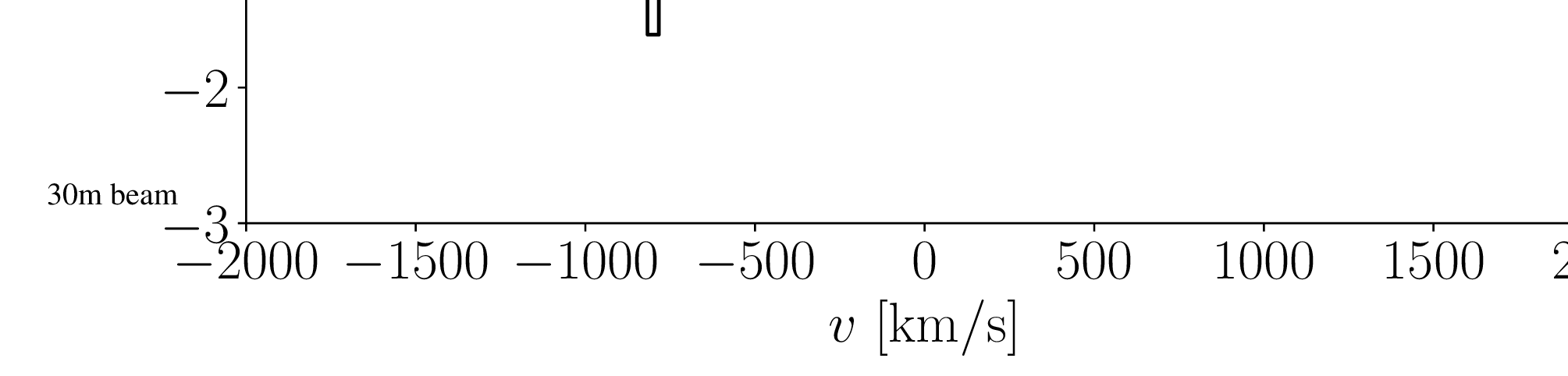
The complementary 30m CO(2-1) observations were intended to assess the overall molecular gas content in the CGr30 group, including possible extended structures in the intra-group medium. As shown in Fig 7, no signal was detected; however, it is still possible to establish an upper limit. Given the median []FWHM of the individual galaxies and the group-scale velocity dispersion derived from the stellar velocities, the expected FWHM of the overall signal is \(\sim 600~\rm km~s^{-1}\). This value further matches the velocity span previously observed for the diffuse []component in this system [60]. Given the RMS noise (\(1.7 ~\rm mJy\) over \(\rm 89.74 ~km s^{-1}\) velocity channels), we evaluate the noise within this FWHM at \(\sigma_{\rm FWHM, 30m}=0.40 ~\rm Jy~km~s^{-1}\), yielding a 3\(\sigma\) integrated line flux upper limit \(F_{\rm upper, 30m} = 1.19 \rm ~Jy~km~s^{-1}\). With the median redshift, luminosity distance, and CO conversion factor, this translates into a 30m total molecular gas mass upper limit \(M_{\rm gas, tot}< 5.4 \times 10^{10}~\rm M_\odot\) (or \(\log M_{\rm gas, tot}<10.73\)).
For comparison with the measurements within galaxies, we stacked the NOEMA spectra weighted by the 30m beam power, assuming a Gaussian beam with an 18half-power beam width. The resulting spectrum is shown in Fig. 8, yielding an integrated line flux of \(0.75 ~\rm Jy ~km~s^{-1}\) with an \(\rm S/N=8.3\). Hence, the CO(2-1) line emission exceeding that of the galaxies in the 30m beam should have an integrated intensity lower than \(0.37 ~\rm Jy ~km~s^{-1}\). Assuming the median redshift, luminosity distance, and CO conversion factor, this flux translates into an overall molecular gas mass in the intra-group medium below \(2\times 10^{10}~\rm M_\odot\), i.e. less than a third of the total gas mass of the large and massive diffuse structure revealed by MUSE, which was estimated to be \(\sim 5 \times 10^{10}~\rm M_\odot\) [60].
4 Conclusion↩︎
In this article, we presented CO(2-1) molecular gas measurements in an over-dense region of a galaxy group at \(z\sim0.7\) using both IRAM’s NOEMA interferometer and 30m telescope. The target group, COSMOS-Gr30, has been chosen among a sample of groups at intermediate redshift that were observed with MUSE to study environmental quenching. It is the densest group of this sample, located at the intersection of large-scale cosmic web filaments, and deep MUSE observations revealed a huge, massive structure of ionized gas wrapping eight galaxies of the group, including one active galactic nucleus (AGN) host. This gas is not pristine and was likely expelled from the galaxies, owing to both internal processes such as star formation and AGN outflows and external processes in the dense environment such as ram pressure stripping and tidal interactions.
With NOEMA, we detected the molecular gas with signal-to-noise ratios \(\rm S/N>5\) in four individual galaxies and derived upper limits in the other 13 galaxies lying within the NOEMA primary beam. We further obtain stacked detections for the total molecular gas content in the 17 galaxies. While some of the group galaxies have typical molecular gas reservoirs, the stacked detections point towards lower molecular gas content within the group galaxies on average, possibly owing to the environmental processes. Indeed, the stacked detection of all galaxies within the NOEMA beam indicates molecular gas masses that are overall \(20-40\%\) of those found in typical star-forming galaxies. Such a depletion suggests that environmental processes in the group are highly efficient at removing or suppressing the molecular gas required for star formation.
With the 30m telescope, we obtained an upper limit for the total molecular gas emission in the beam, which includes most of the extended ionized gas structure uncovered by MUSE. Together with a stacked detection of the molecular gas within the galaxies lying in the 30m telescope beam, this enables us to assess that there is less than \(2\times 10^{10} \rm ~M_\odot\) of molecular gas in the extended gas structure. This suggests that less than a third of the gas displaced from the galaxies into the diffuse structure is in a cold phase.
This article highlights the importance of simultaneously probing gas reservoirs within galaxies and the surrounding intra-group medium to capture environmental quenching in action. In the case of CGr30, the depletion of molecular gas within the galaxies, combined with the presence of an extended gas structure, provides a consistent picture of environmental quenching. However, these processes require further quantification through deeper observations with NOEMA, the IRAM 30m telescope, and ALMA. The latter may also reveal the molecular counterpart of the extended gas structure. Furthermore, more precise SFR measurements are necessary to decrease the uncertainties, and larger samples of target galaxies in groups will allow the assessment of group-to-group variance.
This work is based on observations carried out under project S19BV with the IRAM NOEMA Interferometer and projects 110-19 and 173-20 with the IRAM 30m telescope. IRAM is supported by INSU/CNRS (France), MPG (Germany) and IGN (Spain). We are grateful for the excellent support provided by the IRAM staff. We thank Clotilde Laigle for providing the initial catalogs of realizations of the cosmic web in the COSMOS field, and granting us permission to use them as presented in Appendix 5. D.K. and C.M.-L. acknowledge the support by the Deutsche Forschungsgemeinschaft, DFG project number 4548/4-1. R.H.-C. thanks the Max Planck Society for support under the Partner Group project “The Baryon Cycle in Galaxies” between the Max Planck for Extraterrestrial Physics and the Universidad de Concepción. R.H-C. also gratefully acknowledges financial support from ANID - MILENIO - NCN2024_112 and ANID BASAL FB210003.
5 CGr30 within the cosmic web↩︎
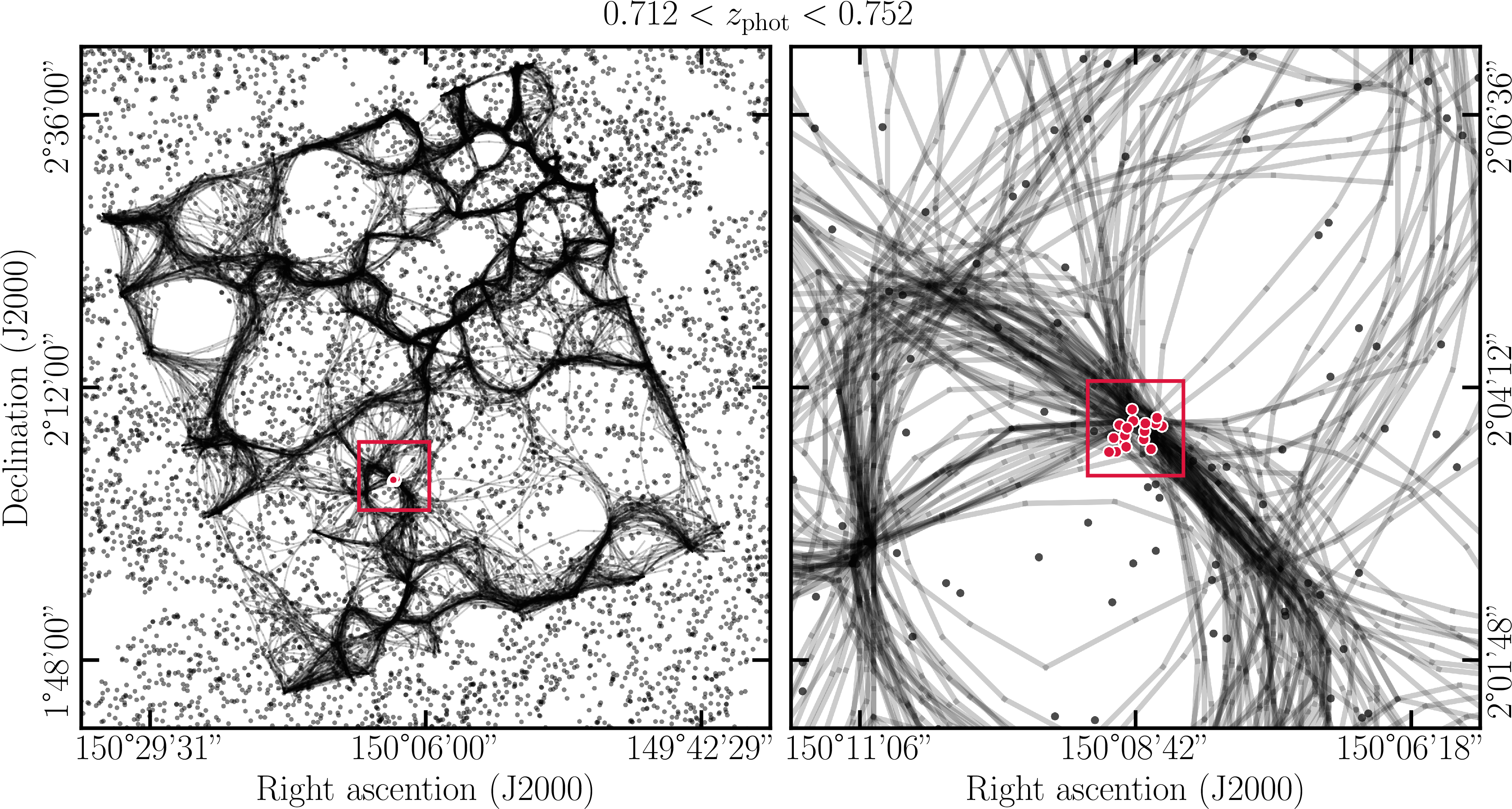
Figure 9 shows the position of CGr30 in the large-scale environment using two dimensional cosmic web reconstructions from the galaxy position field projected along the line of sight using the publicly available software DisPerSE [138], [139].
The cosmic web reconstruction follows the methodology of [140] and [141], using all galaxies in the COSMOS field and tomographic slices with a constant comoving thickness set by the photometric redshift uncertainty of low-mass galaxies in the sample. In COSMOS-Web, the photometric redshift accuracy allows slices with projection depth of \(80\,h^{-1}\,\rm Mpc\). Filaments are identified with DisPerSE at a \(2.5\sigma\) persistence threshold. We refer the reader to [140] for details on the cosmic web reconstructions from DisPerSE [142]. We generate 100 Monte Carlo realizations by sampling photometric redshift probability distributions and propagate these into the filament reconstruction and distance measurements. Mask filling is applied in masked regions by sampling random galaxy positions with an average galaxy number density matching that of the tomographic slice, although the field shown here lies sufficiently far from masked areas so that this correction has a negligible impact.
![Figure 10: Distance to the nearest cosmic web filament, computed as the average over the 100 realisations with Bootstrap errors, as a function of stellar mass for CGr30 galaxies and PHIBSS2 [19] typical star-forming galaxies between z=0.5-0.8 in the COSMOS field, colored according to the molecular gas fraction \mu_{\rm gas}=M_{\rm gas}/M_\star.](/article/2606.26320/images/dfil_mugas.png "fig:")
Fig. 10 displays the distance to the nearest cosmic filament as a function of stellar mass. We compare CGr30 galaxies with the PHIBSS2 sample of typical star-forming galaxies at \(z=0.5-0.8\) in the COSMOS field from [19]. Although the PHIBSS2 galaxies were selected to span the MS scatter without morphological constraints, their relatively regular appearances suggest they are largely isolated systems. The median distance to the nearest filament is \(0.48\) Mpc for the CGr30 galaxies and \(1.45\) Mpc for the PHIBSS2 control sample. As a proof of concept, we explored a possible trend of the molecular gas fraction \(\mu_{\rm gas}=M_{\rm gas}/M_\star\) with distance to the nearest filament. Focusing on the mass range between \(\log M_\star=10.4-11\) where the four CGr30 detected galaxies lie, we find \(\mu_{\rm gas} = 0.23 \pm 0.10\) for the four detected CGr30 galaxies and \(0.28 \pm 0.06\) for the PHIBSS2 galaxies, i.e., no significant trend. To assess the link between molecular gas reservoirs in galaxies and their position with respect to the cosmic web, more observations in well-studied fields such as COSMOS would be needed, spanning different environments. This preliminary exploration of the correlation between gas fraction and distance to cosmic filaments thus further underscores the need for significantly larger samples to yield statistically significant results.
6 Star formation rates from []↩︎
| \({\rm ID}\) | \(F({\rm \oii})\) | \(\log{\rm SFR}_{\rm \oii}\) |
| \([\rm 10^{-18} erg\;s^{-1}\;cm^{-2}]\) | \(\rm[M_\odot \rm yr^{-1}]\) | |
| 49 | \(13.36\) | \(0.09 \pm 0.30\) |
| 57 | ||
| 59 | \(1.28\) | \(0.87 \pm 0.30\) |
| 61 | ||
| 68 | \(24.09\) | \(0.17 \pm 0.30\) |
| 69 | \(16.05\) | \(-0.47 \pm 0.30\) |
| 71 | \(7.90\) | \(1.36 \pm 0.30\) |
| 78 | \(80.77\) | \(-0.74 \pm 0.31\) |
| 82 | \(8.84\) | \(0.28 \pm 0.30\) |
| 93 | ||
| 98 | \(4.22\) | \(1.37 \pm 0.67\) |
| 105 | \(25.20\) | \(0.66 \pm 0.30\) |
| 110 | \(3.10\) | \(0.01 \pm 0.30\) |
| 114 | \(59.83\) | \(-0.45 \pm 0.31\) |
| 119 | \(12.79\) | \(0.75 \pm 0.30\) |
| 123 | ||
| 131 | \(14.26\) | \(1.43 \pm 0.30\) |
![Figure 11: Stacked NOEMA CO(2-1) spectrum for galaxies with []SFR measurements, namely without #57, #61, #93, #123. The corresponding signal yields 1.25\;\rm Jy\;km\;s^{-1} with a \rm S/N = 4.8. The Gaussian fit was carried out imposing its center to be at zero.](/article/2606.26320/_pdflatex/sditcemf.png "fig:")
To assess the sensitivity of our results to the assumed SFR values and their uncertainties, we also derived SFRs from []following [77]. Namely, we
extracted MUSE spectra within apertures of 3in diameter, subtracted the continuum with pPXF, and fitted the []doublet with the 1D function of Camel. We corrected the resulting []luminosities for extinction using the mass-dependent
prescription from [143], [144] for the intrinsic extinction at the rest-frame H\(\alpha\) wavelength and assuming a [145] extinction law with \(R_V=3.1\) for the
Galactic extinction at the []wavelength. Finally, we used the expression from [146] to convert the []luminosities into SFRs. The resulting
values are indicated in Table 3.
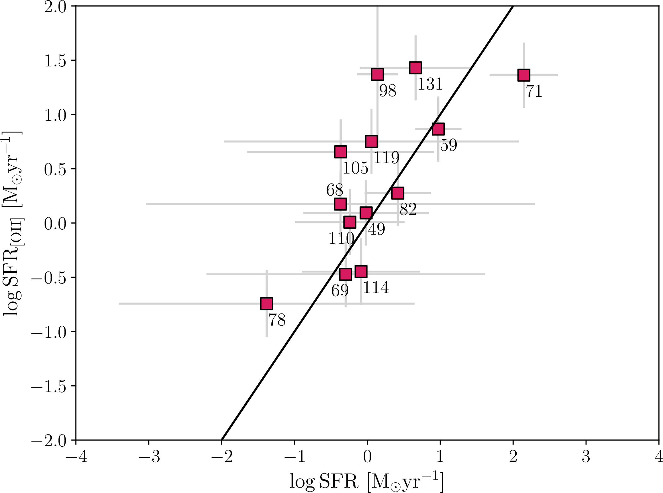
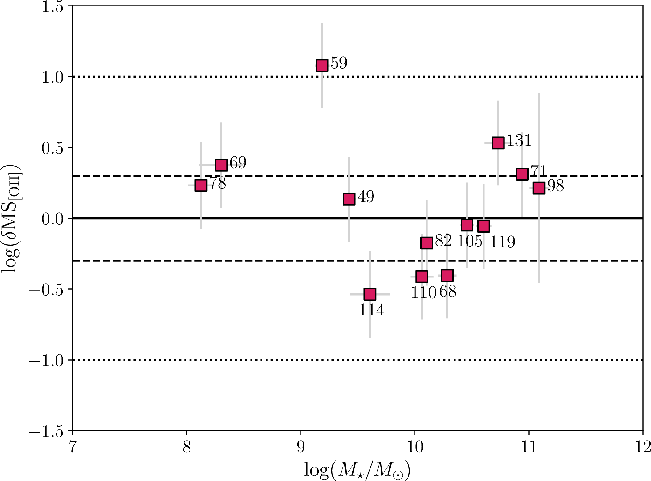
Figure 12: (Left:) Comparison between the SED-based \(\rm SFR\) and \(\rm SFR_{\rm [\ion{O}{ii}]}\) from the []line observed by MUSE. The Pearson correlation coefficient is equal to 0.72. (Right:) Position of the galaxies with respect to the MS, as in Fig. 2 but using the []SFRs instead of the SED-based ones and the MS parametrization of [77] without downward adjustment..
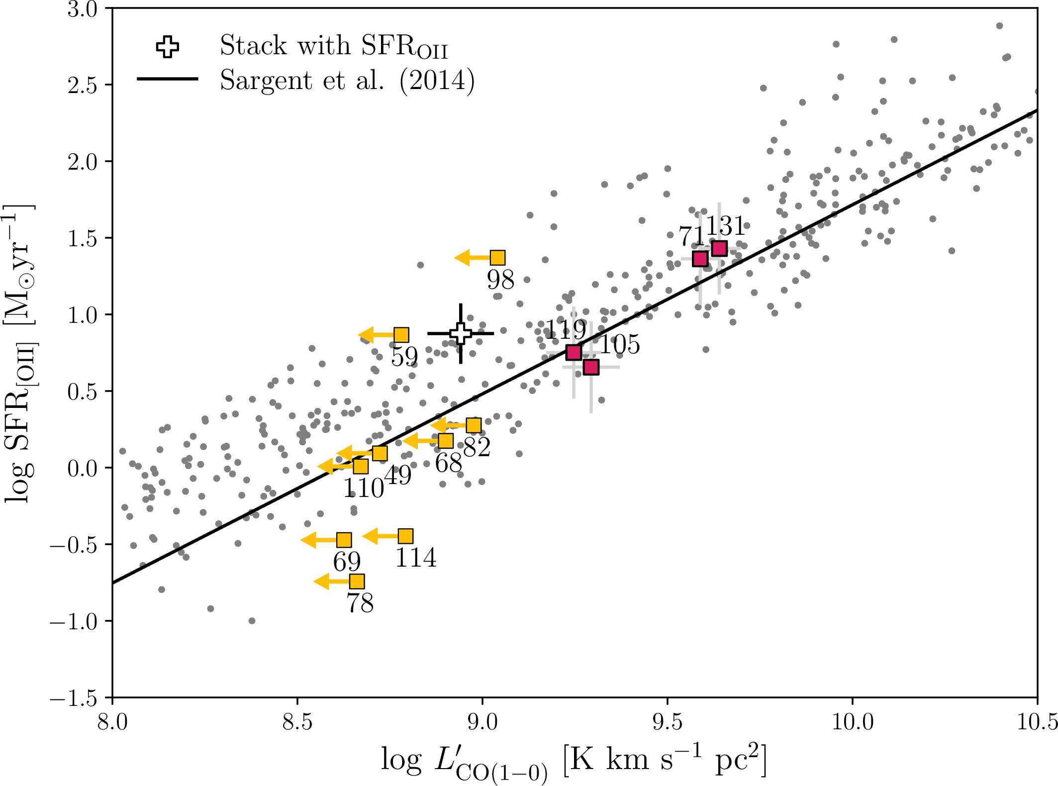
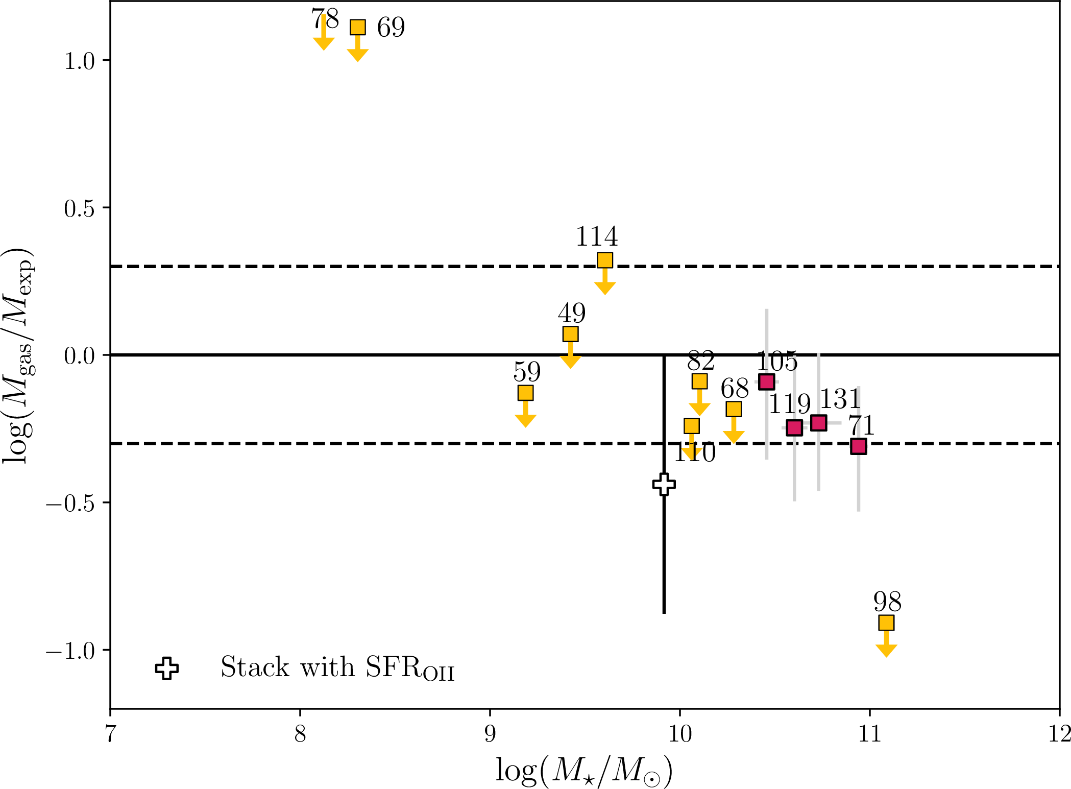
Figure 13: (Left:) Observed relation between \(\rm SFR_{\rm [\ion{O}{ii}]}\) and the intrinsic CO(1-0) luminosity. (Right:) Molecular gas mass divided by that expected from the [105] scaling relations as a function of stellar mass, using the []SFR. On average, the stacked molecular gas mass corresponds to \(0.36\substack{+0.64\\-0.23}\) times the expected value from the scaling relation, and the probability to be below the scaling relation value is 84%. Detected individual galaxies are highlighted in red..
The left panel of Fig. 12 compares the []-based \(\rm SFR_{\rm [\ion{O}{ii}]}\) with the SED-based values. There is an overall linear trend (the Pearson correlation coefficient is equal to 0.72), but differences for individual galaxies and in particular for #71, whose \(\rm SFR_{\rm [\ion{O}{ii}]}\) is significantly lower than the SED-based SFR. Uncertainties in \(\rm SFR_{\rm [\ion{O}{ii}]}\) are assumed to be the combination of the flux uncertainty and a 0.3 dex uncertainty in the conversion factor (which dominates the resulting uncertainty in most cases). The right panel shows the resulting position of the galaxies with respect to the MS, assuming the [77] parametrization of the MS without downward adjustment (since this downward adjustement precisely corresponds to the average offset between []SFRs and SED-based SFRs in the MAGIC sample). Fig. 13 then compares the CO luminosity and the molecular gas mass associated to individual galaxies and stacks with those expected from scaling relations, as in Figs. 5 and 6. Although the individual data points differ from those in these latter figures, the conclusions are similar. In particular, the stacked measurement yields \(0.36\substack{+0.64\\-0.23}\) of the expected value for the molecular gas mass.
7 Star formation histories↩︎
Fig. 14 shows the star formation histories (SFH) of the CGr30 galaxies where available, derived by [87] within
one effective radius. These SFH are obtained as byproducts of pPXF runs on the MUSE data, with the E-MILES stellar population synthesis templates and masked emission lines, see [87] for more details. Interestingly, the SFHs of the four galaxies detected in CO are available and harbor a relatively recent burst of star formation: the three galaxies within the extended
ionized gas structure (#71, #119, #131) underwent a strong burst \(1-2\rm~ Gyr\) ago, while the remaining galaxy (#105) underwent a more limited one 0.5 Gyr ago. The SFH of one other CGr30 galaxy was derived by [87], namely #98, and it contrasts with the previous ones by the absence of any recent burst. Given the group virial radius and velocity dispersion
(\(R_{\rm 200}=669\rm ~kpc\), \(\sigma_g=404~\rm km/s\), see Table 4 of [61]), we
estimate the group dynamical time (\(R_{\rm 200}/\sigma_g\)) to be \(\sim 1.6~\rm Gyr\). The coincidence between the time since the last starburst for the three galaxies in the extended
ionized gas structure and the group dynamical time could suggest that the starburst was triggered by the arrival of the galaxies within the group or a close encounter within it. Simulations and analytical models indeed show that tidal interactions can
trigger starbursts via radial gas inflows, compressive tides and enhanced compressive turbulence leading to an excess of the star-forming dense gas [147]–[149]. However, these tidal interactions typically occur in the denser, inner regions of the group, where local interaction timescales are shorter than the global
dynamical time. The estimated group dynamical time of 1.6 Gyr should thus be viewed as an upper limit for intra-group processing. The fact that the SFR peaks for the three galaxies within the extended ionized gas structure are comparable to this maximum
timescale would then imply that the starbursts predate the galaxies’ entry into the current group core, potentially pointing to pre-processing in smaller subgroups or interactions during the initial assembly phase. We also note that uncertainties in SFHs
derived from full-spectrum fitting increase at older ages, such that broader components fitted at these epochs may reflect these expanding uncertainties rather than prolonged burst durations.
![Figure 14: Star formation histories for the CGr30 galaxies where available, from [87]. For each panel, the black line shows the derived SFR in bins of 0.5 Gyr, the blue solid line the best-fit SFR, and the dashed lines the decomposition into different Gaussian or exponential components. The galaxy index N in the [87] is indicated in the legend. The four galaxies detected in CO (# 71, #105, #119, #131) are characterized by a recent burst of star formation, contrarily to the one that is not detected in CO (# 98).](/article/2606.26320/_pdflatex/wespnrbf.png "fig:")
References↩︎
The []SFRs of [77] and the SED SFRs of [61] were both measured within the same 3apertures, but the []SFRs may be unreliable for CGr30 galaxies lying in the []-emitting diffuse structure because of possible contamination from the structure. Hence our choice to use the SED SFRs of [61] despite their large uncertainties. In Appendix 6, we also consider []SFRs.↩︎
Cf. https://publicwiki.iram.es/Iram30mEfficiencies and in particular the IRAM internal reports [84], Eq. (17), and [85].↩︎
These high values of \(\alpha_{\rm CO}\) affect the corresponding upper limits, but not the stacks, where we consider the median \(\alpha_{\rm CO}\).↩︎
Since the 0.3 dex scatter in \(\mu_{\rm gas}\) is accounted for in their error bars, the stacked data points in Fig. 6 should be compared to the solid line \(y=0\) and not to the dashed lines that highlight the scatter in the relation for individual galaxies.↩︎