Equivariance and Augmentation for Bayesian Neural Networks
June 24, 2026
Abstract
Symmetries are important for many deep learning tasks, ranging from applications in the sciences to medical imaging. However, there is an ongoing debate about whether to impose symmetry constraints on the neural network architecture (yielding
equivariant neural networks) or learn them from augmented training data. Although equivariant networks are well-studied theoretically, much less is known about data augmentation, since analyzing augmentation requires control over the training dynamics.
Inspired by recent results that show that augmented infinite deep ensembles are exactly equivariant, we study data augmentation for Bayesian neural networks (BNNs) trained with variational inference. We focus on variational distributions in the exponential
family and derive conditions under which exact equivariance is reached. We furthermore obtain bounds on the equivariance error and introduce three novel symmetrization techniques which boost the effect of data augmentation in this setting. We conduct
extensive numerical experiments which show that one of our symmetrization methods (orbit expansion) outperforms the baseline in both equivariance and overall performance. Our code is available at github.com/dmw1998/augment-BNNs.
1 Introduction↩︎
In recent years, symmetric learning tasks have become an important field of study. After an initial focus on specialized equivariant networks which impose the symmetry constraints layer-by-layer [1], attention has recently shifted towards learning symmetries from augmented training data [2]. This approach has the advantage of, given an efficient symmetry transformation mechanism, being straightforward to implement and can be used together with highly-optimized and well-performing architectures [3]. However, as the symmetry is merely learned and not imposed, it is only achieved approximately. Therefore, novel techniques are required which improve the symmetry gain derived from augmented training.
![Figure 1: Natural parameters \eta for a variational distribution in the exponential family that lie in H_G correspond to symmetric BNNs, here exemplified with a reflection symmetry. Our main Theorem [thm:equivariance-of-vi] implies that H_G is invariant for augmented training. Through the symmetrization strategies described in Section 3.4, we can increase the equivariance of the final model.](/article/2606.26273/_pdflatex/mpdfhwig.png "fig:")
The explicit layer-wise equivariant neural networks are readily accessible to theoretical analysis, while data augmentation is considerably harder to study since it involves the training dynamics (see the related works section). It is however possible to show that in expectation over initializations, data augmentation leads to exact equivariance [4], [5]. A practical but costly method for approximating such expected values is training a deep ensemble.
The purpose of this work is to investigate a cheaper way to realize such “equivariance in expectation”: Training Bayesian neural networks (BNNs) with variational inference on augmented data. In this setting, sampling from the posterior predictive distribution replaces the inference step on the ensemble and yields Bayesian uncertainty estimates. In this setting, only one training run is necessary to obtain the variational posterior, in contrast to the one training run per ensemble member for deep ensembles. Furthermore, since BNNs show stable out of distribution behavior, they are particularly well suited for small datasets, the regime in which data augmentation can be expected to have the largest effect.
Our main contributions are the following:
We study BNNs trained on augmented data with a variational distribution from the exponential family. We show that, when the training starts from an invariant prior, the variational distribution stays invariant throughout training, under some mild assumptions. This generalizes a similar result from [6] for non-Bayesian network training.
We derive bounds for the deviation of the variational distribution from equivariance if the prior is not equivariant. We furthermore prove bounds for the equivariance error in the predictions due to finite sampling. These theoretical results are validated numerically.
We introduce three symmetrization methods (geometric averaging, projection and orbit expansion) that can be applied during training to improve the equivariance properties of the BNN. We test these techniques in extensive numerical experiments for image classification. Orbit expansion outperforms the baseline in both model performance and equivariance.
2 Related Work↩︎
2.0.0.1 Equivariant neural networks.
The issue of symmetry, i.e. invariance and equivariance, of deep neural nets has grown into an entire subfield called geometric deep learning [1]. The most prominent construction of equivariant networks is the layerwise one. This strategy originates from GCNNs, Group Convolutional Neural Networks [7], but has by now been generalized to virtually any symmetry induced by any group [8]–[10]. There are also other strategies, such as learning from invariants [11], frame averaging [12], fundamental domain projection [13] and group averaging. There are also works in which symmetries are enforced approximately, for instance through so called weight annealing [14].
2.0.0.2 Augmentation and training dynamics.
The question of the effect of data augmentation on the training dynamics of neural networks have been treated in several simplified contexts, such as feature averaged models [15], [16] as well as linear neural networks [17]–[19]. In these cases, it is often possible to prove equivalence of augmentation and equivariance. Fully non-linear networks were treated in [6], [20], whose results we generalize to Bayesian networks here.
Empirical studies on the difference between augmentation and restrictions are plentiful. More systematic treatments are [21]–[23].
2.0.0.3 Bayesian neural networks.
Bayesian approaches to deep learning have been studied for many years [24] since they offer uncertainty estimates for neural networks that are otherwise black-box models (see the PhD thesis by [25] for an overview). However, making BNNs practically applicable requires integrating variational inference into the deep learning training methodology [26]–[28]. For a review of BNNs with a focus on practical applications, see [29].
Not many prior works consider symmetries in relation to BNNs. [30] propose a probabilistic group-averaging of BNNs in order to realize a soft symmetry constraint, optimized on the data. Closest to our work is [31] which uses a specific prior that combines different weight-sharing schemes and therefore symmetry constraints. During training, the network learns which symmetry fits the data best. In contrast, we consider training on augmented data with a generic prior that does not impose weight-sharing.
3 Theory↩︎
We develop a theoretical framework for understanding how data augmentation induces equivariance in variational Bayesian inference. We proceed in three steps: first, we characterize when exponential families are closed under group actions (3.2); second, we show that data-augmented training makes the ELBO invariant, and how that affects the training (3.3); third, we propose symmetrization mechanisms and analyze their properties (3.4).
3.1 Preliminaries↩︎
In this section, we introduce the mathematical tools used throughout this paper. We begin with exponential families, which provide the structural backbone for our theoretical analysis, before reviewing variational inference and the group theoretic concepts needed to formalize symmetry.
3.1.0.1 Exponential families.
An exponential family of probability distributions is defined through a base measure \(h(\theta)\), a sufficient statistic \(T(\theta)\in \mathbb{R}^k\) and a log-partition function \(A(\eta)~:=~\log~\int~h(\theta) \exp(\eta^{\top} T(\theta)) d\theta\). A distribution belongs to the exponential family if its density has the form \[q_{\eta}(\theta) = h(\theta) \exp(\eta^{\top} T(\theta) - A(\eta))\,,\] where \(\eta\in H \subseteq \mathbb{R}^k\) is the natural parameter. Examples of such families include normal, exponential and log-normal distributions. An exponential family \(\mathcal{Q} := \{q_{\eta}(\theta) \mid \eta \in H\}\), is regular if \(H\) is open, and minimal if the components of \(T(\theta)\) are linearly independent.
3.1.0.2 Group actions and push-forward distributions.
We assume that a group \(G\) acts on the input space \(\mathcal{X}\), the output space \(\mathcal{Y}\), and the parameter space \(\Theta\) via representations \(\rho_{\mathcal{X}}\), \(\rho_{\mathcal{Y}}\), and \(\rho_{\Theta}\) respectively. Throughout, we assume that \(\rho_{\Theta}\) is compatible with the data representations \(\rho_{\mathcal{X}}\) and \(\rho_{\mathcal{Y}}\) in the following sense: \[\label{eq:compatibility} f(\rho_\mathcal{X}(g)x;\theta) = \rho_\mathcal{Y}(g)f(x;\rho_\Theta(g)^{-1}\theta).\tag{1}\] Following the layered decomposition \(\Theta = \bigoplus_{\ell} \Theta_{\ell}\) of a neural network’s parameters, we assume that \(\rho_{\Theta}\) acts per layer, i.e., \(\rho_{\Theta} = \bigoplus_{\ell} \rho_{\Theta_{\ell}}\). There is a canonical construction of such a \(\rho_\Theta\): One introduces representations \(\rho_{\Theta_{\ell}}\) on the hidden layers and then imposes equivariance on each linear layer with respect to the two representations acting on the input and output of that layer. As long as the non-linearities are equivariant with respect to the same representations (which is always the case for pointwise non-linearities and permutation representations) one obtains (1 ). For more details, see [6]. The choice of \(\rho_{\Theta}\), or equivalently the choice of the hidden layer representations, is a modeling decision that we revisit in 3.4. When there is no risk of confusion, we write \(gx\) and \(gy\) as shorthands for \(\rho_{\mathcal{X}}(g)x\) and \(\rho_{\mathcal{Y}}(g)y\), but retain the explicit notation \(\rho(g)\theta\) for the parameter space, where the representation structure is central to our analysis. The push-forward of a distribution \(q\) under \(g \in G\) is defined as \[\mathcal{T}_{g} \# q(B) := q(\rho(g)^{-1} B)\] for any measurable set \(B\), with density \(\mathcal{T}_{g} \# q (\theta) = q(\rho(g)^{-1} \theta) \left|\det D(\rho(g)^{-1}) (\theta)\right|\). A distribution \(q\) is called \(G\)-invariant if \(\mathcal{T}_{g} \# q = q\) for all \(g \in G\).
3.1.0.3 Bayesian neural networks (BNN) and variational inference (VI).
A neural network is a parametrized function \(f(\cdot; \theta): \mathcal{X} \rightarrow \mathcal{Y}\). They define conditional label distributions \(p(y\, \vert \, x, \theta) = p(y\, \vert \, f(x;\theta))\). In the Bayesian treatment, we put a prior \(p_{0}(\theta)\) on the weights and calculate the posterior \(p(\theta \mid \mathcal{D})\) given a dataset \(\mathcal{D} = \{(x_{i}, y_{i})\}_{i=1}^{N_{0}}\) via Bayes’ rule. However, since the posterior neural network likelihood typically is intractable, one makes a variational inference approximation \(q_\eta \in \mathcal{Q}\), and then choose the parameters \(\eta\) to maximize the evidence lower bound [32] \[\mathrm{ELBO}(\eta) := \mathbb{E}_{q_{\eta}} [\log p(\mathcal{D} \mid \theta)] - D_{\mathrm{KL}}(q_{\eta} \Vert p_{0})\,. \label{eq:elbo}\tag{2}\] The posterior predictive is approximated by Monte Carlo sampling from \(q_\eta\): \[F_\eta(x) := \mathbb{E}_{\theta \sim q_{\eta}} [f(x;\theta)] \approx \frac{1}{T}\sum_{t=1}^{T} f(x;\theta^{(t)})\,, \quad \theta^{(t)} \sim q_\eta\,. \label{eq:post-predictive}\tag{3}\]
3.1.0.4 Data augmentation.
Given a finite group \(G\) and a dataset \(\mathcal{D} = \{(x_{i}, y_{i})\}_{i=1}^{N_{0}}\) drawn i.i.d. from a data distribution \(P_{\mathcal{X}}\), data augmentation constructs an augmented dataset \(\mathcal{D}_{\mathrm{aug}} = \{(gx_{i}, gy_{i}) \mid g \in G, (x_{i},y_{i}) \in \mathcal{D}\}\), expanding the dataset by a factor of \(|G|\). One could also consider a continuous compact group by sampling finitely many Haar-distributed group elements. This comes with some subtleties that we discuss in [app:continuous-compact-groups]. In the following, we instead restrict to the case of finite \(G\). Following the mini-batch scaling convention of [26] and [27], instead of using the ELBO (2 ) directly, we work with a \(\beta\)-weighted objective: \[\mathcal{L}_{\beta}(\eta) := \underbrace{\tfrac{1}{N}\,\mathbb{E}_{q_{\eta}}[-\log p(\mathcal{D}_{\mathrm{aug}} \mid \theta)]}_{=:\,R_{\mathrm{aug}}(\eta)} + \beta D_{\mathrm{KL}}(q_{\eta} \Vert p_{0}), \label{equ:L-beta}\tag{4}\] where \(N = |G| \cdot N_{0}\) is the augmented dataset size. \(\mathcal{L}_{\beta}\) with \(\beta = 1/N\) is the rescaled negative ELBO.
If we assume the following invariance of the forward model: \[\label{eq:forward95invariance} p(gy \, \vert \, gf(x;\theta)) = p(y\, \vert \, f(x;\theta)),\tag{5}\] the compatibility of \(\rho_{\Theta}\) with the data representation implies that the augmented likelihood inherits the symmetry of the data. Note that condition (5 ) is weak – it is e.g. satisfied for \(y\sim f(x;\theta) +e\) for a \(G\)-invariant error \(e\) – and furthermore independent of the architecture \(f\).
propositionrestateinvariantlikelihood Let \(L_{\mathrm{aug}}(\theta) := p(\mathcal{D}_{\mathrm{aug}}\mid\theta)\) be the likelihood of the augmented dataset. Under the compatibility assumption (1 ) as well as the invariance assumption (5 ), the likelihood is \(G\)-invariant: \[L_{\mathrm{aug}}(\rho(g)^{-1}\theta)=L_{\mathrm{aug}}(\theta),\, \forall g \in G,\, \theta \in \Theta\,.\]
The proof is given in [app:proof-of-prop-invariant-augmented-likelihood].
3.1.0.5 Equivariance.
A single network \(f(\cdot\,;\theta)\) is \(G\)-equivariant if \(f(gx;\theta) = g f(x;\theta)\) for all \(x \in \mathcal{X}\), \(g \in G\). More generally, the predictive map \(F_\eta\) defined in (3 ) is \(G_\varepsilon\)-equivariant if the equivariance defect \(\Delta^{\mathrm{eq}}_{F}(\eta)\) is bounded by \(\varepsilon\), \[\Delta^{\mathrm{eq}}_{F}(\eta) := \mathbb{E}_{x \sim P_{\mathcal{X}},\, g \sim \nu_{G}}\!\left[\left\|F_{\eta}(gx) - g F_{\eta}(x)\right\|^{2}\right] \leq \varepsilon.\] Here, \(\nu_G\) denotes the normalized Haar measure on \(G\). When \(\varepsilon = 0\), this reduces to exact \(G\)-equivariance of \(F_\eta\) \(P_\mathcal{X}\)-a.s. One central question is whether minimizing \(\mathcal{L}_\beta\) on \(\mathcal{D}_\mathrm{aug}\) drives \(\Delta^\mathrm{eq}_F(\eta)\) to zero, and at what rate.
3.2 Closed exponential family under group actions↩︎
Neural networks can learn equivariance efficiently from augmented data only when the parameter space is closed under group transformations [6]. Similarly, in the Bayesian setting, we restrict the variational family to those closed under group transformations. As the following theorem shows, this imposes constraints on the exponential family. We provide the proof in [app:proof-of-thm-closure-under-push-forward].
theoremrestateclosure A regular minimal exponential family \(\mathcal{Q}\) is closed under the push-forward operator \(\mathcal{T}_{g}\) for all \(g \in G\) if and only if for each \(g\) there exist \(M_{g} \in \mathbb{R}^{k \times k}\), \(d_{g} \in \mathbb{R}^{k}\), \(b_{g} \in \mathbb{R}^{k}\) and \(c_{g} \in \mathbb{R}\) such that for all \(\theta \in \Theta\), \[\begin{align} T(\rho(g)^{-1} \theta) &= M_{g} T(\theta) + d_{g}, \\ h(\rho(g)^{-1} \theta) \left|\det D(\rho(g)^{-1})(\theta)\right| &= h(\theta) \exp(b_{g}^\top T(\theta) + c_{g}). \label{eq:base95measure} \end{align}\tag{6}\] When these conditions hold, \(\mathcal{T}_{g} \# q_{\eta} = q_{\eta_{g}}\) where \(\eta_{g} = M_{g}^\top\eta + b_{g}\), and the transformation \(\phi_{g}: \eta\mapsto M_{g}^\top\eta + b_{g}\) forms an affine action of \(G\) on the space of natural parameters \(H\).
A family \(\mathcal{Q}\) is hence closed if and only if there exists an affine representation of the group acting on the ambient space \(\mathbb{R}^k\) of the space of natural parameters, that makes \(T: \Theta \to \mathbb{R}^k\) invariant, and with respect to which the base measure transforms according to (6 ).
Example 1 (Mean-field Gaussian under permutation actions). Consider the mean-field Gaussian family \(\mathcal{Q} = \{\mathcal{N}(\mu, \mathrm{diag}(\sigma^{2})): \mu \in \mathbb{R}^{d}, \sigma^{2} \in \mathbb{R}^{d}_{>0}\}\) on \(\Theta = \mathbb{R}^{d}\). This family has sufficient statistic \(T(\theta) = (\theta,\,\theta \odot \theta) \in \mathbb{R}^{d}\oplus \mathbb{R}^d\), constant base measure \(h(\theta) = (2 \pi)^{-d/2}\), and natural parameter \(\eta = (\eta_{1}, \eta_{2})\in\mathbb{R}^{d}\oplus \mathbb{R}^d\) given by \((\eta_{1})_{i} = \mu_{i} / \sigma_{i}^{2}\) and \((\eta_{2})_{i} = -1/(2 \sigma_{i}^{2})\).
Let \(G\) act on \(\Theta\) by a permutation representation \(\rho(g) = R_{g}\). Then, both conditions of [thm:closure-under-push-forward] are met: Permutation matrices commute with the Hadamard product, so \(T(R_{g}^{-1} \theta) = (R_{g}^{-1} \oplus R_{g}^{-1})T(\theta)\) giving \(M_{g} = R_{g}^{-1} \oplus R_{g}^{-1}\) and \(d_{g} = 0\). Since \(|\det R_{g}^{-1}| = 1\) and \(h\) is constant, (6 ) is fulfilled by \(b_{g} = c_{g} = 0\). Using \((R_{g}^{-1})^{\top} = R_{g}\), the induced natural-parameter transformation is \[\phi_{g}(\eta) = M_{g}^{\top} \eta = (R_{g} \oplus R_{g}) \eta,\] which simply amounts to permuting the entries of \(\eta_{1}\) and \(\eta_{2}\). Equivalently, \[\mathcal{T}_{g} \# \mathcal{N}(\mu, \mathrm{diag}(\sigma^{2})) = \mathcal{N}(R_{g} \mu, \mathrm{diag}(R_{g} \sigma^{2})),\] so the family is indeed closed.
3.3 Data augmentation induces equivariance↩︎
The representation \(\phi_g\) fixes the set of symmetric parameters \(H_G : = \{\eta \in H \, \vert \, \phi_g(\eta)=\eta, \, \forall \, g\in G\}\). Just as in the single network case, parameters in \(H_G\) correspond to equivariant predictive maps.
Proposition 1. For \(\eta\in H_G\), \(F_\eta\) is \(G\)-equivariant.
Proof. If \(\eta\in H_G\), \(\mathcal{T}_{g} \# q_{\eta} =q_{\phi_{g}(\eta)}=q_{\eta}\). Hence, if \(\theta \sim q_\eta\), \(\rho(g)\theta\sim q_{\eta}\) for every \(g\in G\). This together with the compatibility assumption implies that \(f(gx;\theta) =gf(x;\rho(g^{-1})\theta)\stackrel{\mathrm{d}}{=} gf(x;\theta)\), where the last equality is in distribution. Taking the expectation over \(\theta\) yields \(F_\eta(gx)=gF_\eta(x)\), which is the claim. ◻
Our main result states that, under the conditions presented below, \(H_{G}\) is invariant under gradient descent on augmented data. Initializing \(\eta\) there guarantees equivariant \(F_\eta\) throughout training.
Assumption 1 (Invariant prior). The prior \(p_{0} = q_{\eta_{0}}(\theta)\) for some \(\eta_{0}\) is \(G\)-invariant, i.e., \(\mathcal{T}_{g} \# p_{0} = p_{0}\) for all \(g \in G\), or equivalently \(\phi_{g}(\eta_{0}) = \eta_{0}\).
Assumption 2 (Volume-preserving action). \(|\det D(\rho(g)^{-1})(\theta)| = 1\,\) for all \(g \in G\) and \(\theta \in \Theta\).
Both these assumptions are natural: an invariant prior matches the hypothesis of a \(G\)-symmetric task, and volume-preservation is automatic for the, in practice very common, orthogonal actions.
theoremrestateequivariance 1 2 imply the following for variational inference using invariant likelihoods and closed exponential families:
Loss invariance. The loss \(\mathcal{L}_{\beta}\) is invariant under the natural parameter transformation: \[\mathcal{L}_{\beta}(\eta) = \mathcal{L}_{\beta}(\phi_{g}(\eta)), \quad \forall g \in G,\, \eta \in H.\]
Gradient equivariance and update commutativity. The gradient of the loss \(\mathcal{L}_{\beta}\) satisfies \[\nabla_{\eta} \mathcal{L}_{\beta}(\phi_{g}(\eta)) = M_{g}^{-1} \nabla_{\eta} \mathcal{L}_{\beta}(\eta), \quad \forall g \in G,\, \eta \in H.\] Consequently, for \(M_{g}\) orthogonal, gradient descent \(\mathcal{U}(\eta) = \eta - \alpha \nabla_{\eta} \mathcal{L}_{\beta}(\eta)\) commutes with \(\phi_{g}\): \[\label{eq:update95commute} \mathcal{U}(\phi_{g}(\eta)) = \phi_{g}(\mathcal{U}(\eta)).\tag{7}\]
Invariant subspace is preserved. For \(M_{g}\) orthogonal, the equivariant subspace \(H_{G}\) is preserved by gradient updates: if \(\eta^{(0)} \in H_{G}\), then \(\eta^{(t)} \in H_{G}\) for all \(t \geq 0\).
Optimal solutions inherit symmetry. The set of optimal natural parameters \(H^{\ast} = \arg\min_{\eta} \mathcal{L}_{\beta}(\eta)\) is closed under \(\phi_{g}\) for all \(g \in G\). If the optimum is unique, then \(\phi_{g}(\eta^{\ast}) = \eta^{\ast}\).
The proof is given in [app:proof-of-thm-equivariance-of-vi]. This formalizes the intuition behind data augmentation: by making the training objective symmetric, augmentation ensures that \(H_G\) is invariant – and in the case of a unique minimum, even that the minimum is in \(H_G\).
Note that Theorem [thm:equivariance-of-vi] does not rely on augmented data directly, only on an invariant likelihood (which is implied by data augmentation according to Proposition [prop:invariant-augmented-likelihood]). Therefore, the theorem is still applicable when the symmetry is present in the data but unknown. However in such a case, it is hard to guarantee that the prior is invariant. The next theorem, which we prove in [app:proof-of-thm-prior-independent-convergence], shows that as the dataset size increases, the effect of a non-invariant prior vanishes.
theoremrestateconvergence Assume 2, and that the likelihood is invariant. Let \(R^{\ast}_{\mathrm{aug}}:= \inf_{\eta}R_{\mathrm{aug}}(\eta)\) and \(\eta^{\ast}_{\beta}(p_{0})\in\arg\min_{\eta}\mathcal{L}_{\beta}(\eta; p_{0})\). We then have \[R_{\mathrm{aug}}(\eta^{\ast}_{\beta}(p_{0})) \leq R^{\ast}_{\mathrm{aug}} + \beta \cdot C(p_{0}),\] for any prior \(p_{0}\), where \(C(p_{0}) := \inf_{\eta^{\ast} \in H^{\ast}_{R}} D_{\mathrm{KL}}(q_{\eta^{\ast}} \Vert p_{0})\) and \(H^{\ast}_{R} := \arg\min_{\eta} R_{\mathrm{aug}}(\eta)\) is the set of risk-optimal natural parameters. As \(\beta \to 0\), all minimizers achieve \(R^{\ast}_{\mathrm{aug}}\) regardless of the prior.
Note that the quantity \(C(p_{0})\) measures how well the prior aligns with the risk-optimal orbit. Since \(\beta = 1/N\), with sufficient data, it becomes irrelevant. In contrast, \(R_{\mathrm{aug}}\) is asymptotically constant; It will almost surely converge to the true likelihood \(\mathbb{E}_{\substack{(x,y)\sim P_{\mathcal{X}}}}\mathbb{E}_{g\sim \nu_G}\mathbb{E}_{q_{\eta}}[-\log p((gx,gy) \mid \theta)]\).
Next, we address the fact that the true predictive maps \(F_\eta\) in practice must be approximated with finite sample means. This will indeed cause a Monte Carlo equivariance defect \(\widehat{\Delta}^{\mathrm{eq}}_{F}(\eta)\) (defined formally in ([equ:def-delta-hat])), but that defect vanishes with a number of samples grows, at the expected rate, as the following theorem shows (proof in [app:proof-of-thm-complexity-for-G-e-equivariance]). We verify it and [thm:prior-independent-convergence] in 4.1.
theoremrestatecomplexity Suppose \(f(x;\theta)\) is uniformly bounded in \(x \in \mathcal{X}\) and \(q_{\eta}\)-a.s.in \(\theta\), and that the \(G\)-action on \(\mathcal{Y}\) is orthogonal. Then there exist constants \(C_{\mathrm{data}}\) and \(C_{\mathrm{weight}}\) such that, for any fixed \(\eta\), with probability at least \(1-\delta\) over the \(N_0\) i.i.d.inputs \(x_i \sim P_\mathcal{X}\) and the \(T\) i.i.d.posterior samples \(\theta^{(t)} \sim q_\eta\), the Monte Carlo equivariance defect satisfies \[\widehat{\Delta}^{\mathrm{eq}}_{F}(\eta) \leq \Delta^{\mathrm{eq}}_{F}(\eta)+ C_{\mathrm{data}}\sqrt{\frac{\log(2/\delta)}{N_{0}}} + C_{\mathrm{weight}}\sqrt{\frac{\log(2/\delta)}{T}}\,.\] In other words, for any \(\varepsilon_{0},\varepsilon_{\mathrm{data}}, \varepsilon_{\mathrm{weight}} >0\), if \(\Delta_F^{\mathrm{eq}}(\eta)<\varepsilon_0\), it suffices to choose \[N_{0} \ge \frac{C_{\mathrm{data}}^{2}}{\varepsilon_{\mathrm{data}}^{2}}\log\left(\frac{2}{\delta}\right), \quad T \ge \frac{C_{\mathrm{weight}}^{2}}{\varepsilon_{\mathrm{weight}}^{2}}\log\left(\frac{2}{\delta}\right)\] in order for \(\widehat{\Delta}_F^{\mathrm{eq}}(\eta) < \varepsilon_0 + \varepsilon_{\mathrm{data}}+\varepsilon_{\mathrm{weight}}\) with probability at least \(1-\delta\).
3.4 Symmetrization of the variational posterior↩︎
According to [thm:equivariance-of-vi](iii), the space of parameters corresponding to equivariant variational distributions \(H_{G}\) is preserved during training. Hence, if we ensure that the parameters lie in \(H_{G}\) at some point during training, we will arrive at an equivariant variational posterior at the end of it. Therefore, we propose two complementary mechanisms that place \(\eta\) into \(H_{G}\), one by projecting an existing posterior, one by constructing the posterior from a smaller base, see Figure 1.
3.4.0.1 Orbit averaging.
Given a posterior distribution \(q_{\eta}\) at any point during training, we construct a \(G\)-invariant posterior by averaging its natural parameter over the orbit: \[\tilde{\eta} = \frac{1}{|G|} \sum_{g \in G} \phi_g(\eta). \label{equ:orbit-average}\tag{8}\] We can interpret this operation in two ways: First, \(\tilde{\eta}\) is the natural parameter of the geometric mean distribution \(\tilde{q}(\eta) \propto \left[\prod_{g \in G} \Big(\mathcal{T}_{g} \# q_{\eta}\Big)(\theta)\right]^{\frac{1}{|G|}}\) (which lies in \(\mathcal{Q}\) by [lmm:geometric-mean-invariance-and-membership] in [app:geometric-averaging-stays-in-Q]). Secondly, for orthogonal \(\phi_g\), \(\tilde{\eta}\) is the orthogonal projection of \(\eta\) onto the invariant subspace \(H_{G}\) under the Euclidean inner product – this in particular shows that \(\tilde{\eta}\in H_G\).
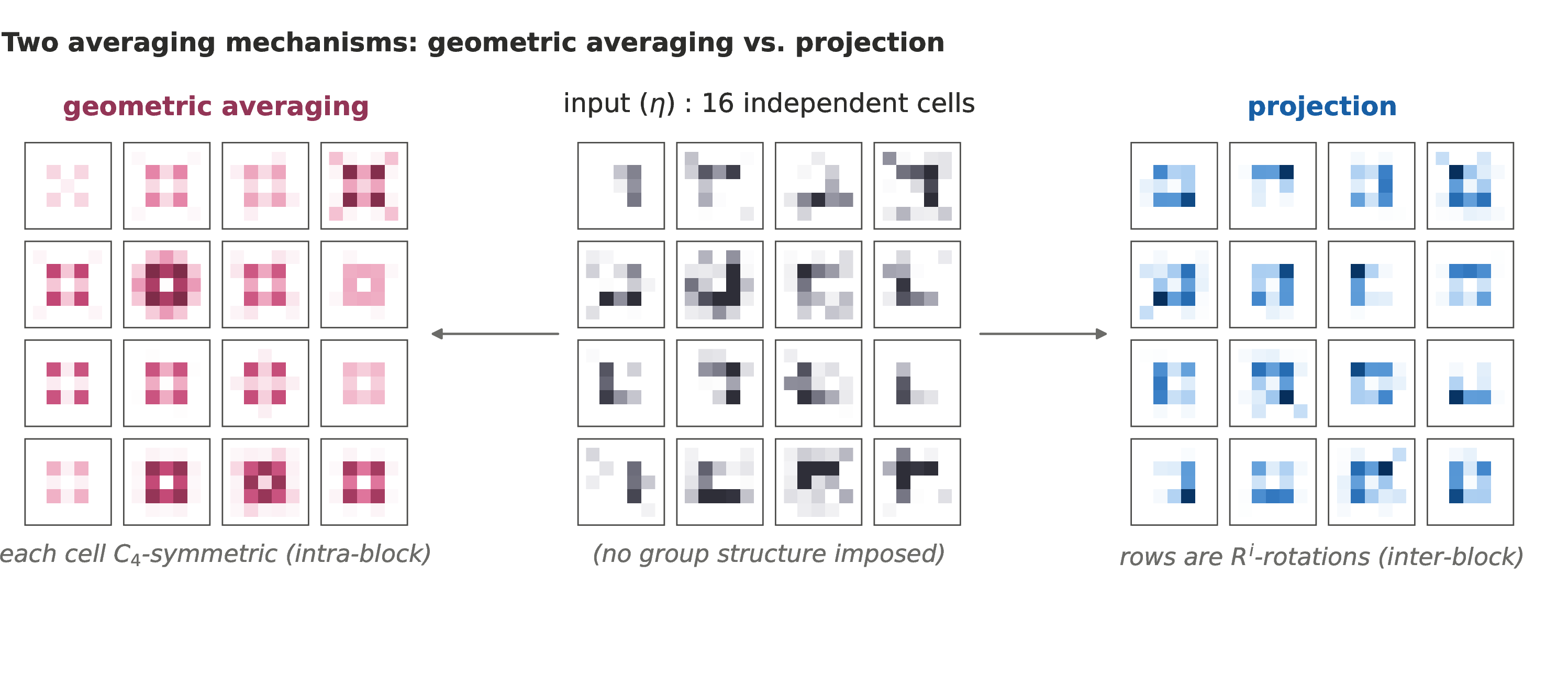
The mechanism specializes through the choice of \(\rho_{\Theta}\). Let us exemplify this in the case of \(C_4\) acting on convolutional layers: First, we can define a representation acting by rotating each individual convolutional channel and secondly a representation that additionally permutes channel blocks, inspired by group convolutional neural (GCNNs) from [7]. The corresponding average operations on the filters are depicted in Figure 2. We will refer to the former as geometric averaging, and the latter as projection. We derive both in detail in [app:symmetrization-strats].
3.4.0.2 Orbit expansion.
Instead of symmetrizing a general parameter of the intended size, we can also first train a small parameter and then, in a manner inspired by the weight-sharing structure of
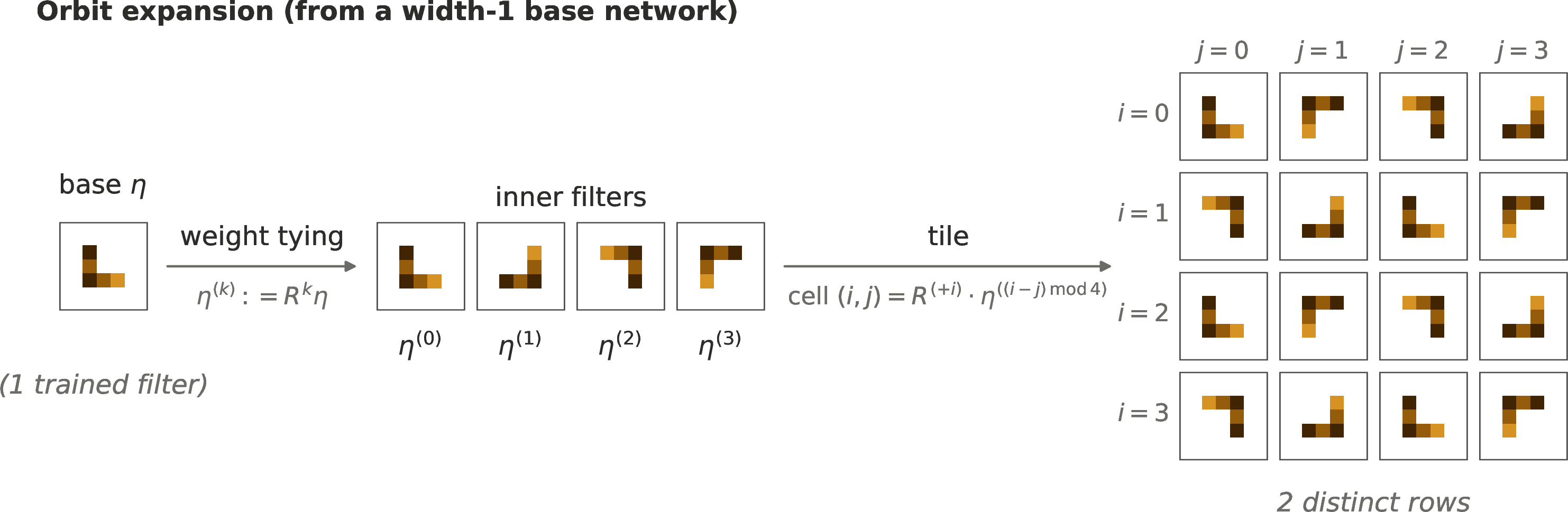
GCNNs, extend it to an equivariant one of bigger size. Concretely, a base network with \(1/|G|\) of the target channel width is trained in Stage 1, yielding a posterior \(q_{\eta_{\mathrm{small}}}\). At the start of Stage 2, the network is expanded to full width by inserting rotated versions of each filter in \(|G|\times |G|\)-blocks (see 3). We refer to this strategy as orbit expansion. The resulting posterior \(q_{\eta_{\mathrm{full}}}\) has a \(G\)-equivariant
block structure at the parameter level. In [app:expansion-along-orbit-filter-arrangement-ablation], we compare three different expansion strategies.
4 Experiments↩︎
In our experiments, we consider the cyclic group \(C_4\) of rotations of multiples of \(90^{\circ}\) acting on FashionMNIST [33]. This setup allows us to augment exactly and enables extensive Monte Carlo sampling. Throughout our experiments, we
use Gaussian variational distributions which satisfy the constraints of Theorem [thm:closure-under-push-forward]. In Appendix [app:variational-family-closure-ablation], we provide additional ablations for other variational distributions. Code is
provided at github.com/dmw1998/augment-BNNs.
4.1 Validation of Theorems↩︎
We start by verifing the predictions of [thm:prior-independent-convergence] [thm:complexity-for-G-e-equivariance]. We use a Bayesian neural network with two convolutional layers and one linear layer and vary the dataset size \(N_{0} \in \{500,\,5000,\,20000,\,50000\}\). For [thm:prior-independent-convergence], we compare an invariant isotropic Gaussian prior \(p_{0} = \mathcal{N}(0,I)\) against a non-invariant prior with means drawn from a normal distribution. Posterior predictives are estimated with \(T\) Monte Carlo samples. The results are presented in 4.
![Figure 4: Empirical validation of [thm:prior-independent-convergence] [thm:complexity-for-G-e-equivariance]. (a) The empirical equivariance defect decreases with N_{0} under both invariant and random Gaussian priors, and the two curves converge. (b) K-fold standard deviation of the Monte Carlo estimate \widehat{\Delta}^{\mathrm{eq}}_F(\eta; T) across K=10 independent runs at each T. The decay matches the \mathcal{O}(1/\sqrt T) rate predicted by [thm:complexity-for-G-e-equivariance] (dotted reference line, slope -0.5). (c) The training gap decreases with N_{0} in close agreement with the 1/\sqrt{N_{0}} rate predicted by [thm:complexity-for-G-e-equivariance]. The dashed line is a fit with empirical constant C_{\mathrm{data}} \approx 1.95. Error bars are \pm 1 s.d. across 5 seeds.](/article/2606.26273/plots/theorem_validation.png "fig:")
4.1.0.1 Priors.
The empirical defect \(\widehat{\Delta}^{\mathrm{eq}}_{F}\) decreases monotonically with \(N_{0}\) under both priors, from \(0.057 \pm 0.007\) to \(0.033 \pm 0.001\) (invariant) and \(0.088 \pm 0.003\) to \(0.035 \pm 0.001\) (random); the two curves converge as \(N_{0}\) grows, consistent with [thm:prior-independent-convergence].
4.1.0.2 Monte Carlo complexity.
[thm:complexity-for-G-e-equivariance] predicts that the gap between the \(T\)-sample Monte Carlo estimate \(\widehat{\Delta}^{\mathrm{eq}}_{F}(\eta;T)\) and the true predictive map decays as \(\mathcal{O}(1/\sqrt{T})\). We assess this directly by drawing \(K=10\) independent \(T\)-sample estimates at each \(T\) and tracking their standard deviation across the \(K\) runs. The results are shown in 4 (b). The theorem is indeed verified: a \(\log\)-\(\log\) fit of the \(K\)-fold std against \(T\) yields slopes of \(-0.45\), \(-0.66\), \(-0.52\), \(-0.51\) for \(N_{0} \in \{500,\,5000,\,20000,\,50000\}\) respectively, all close to the predicted \(-0.5\).
4.1.0.3 Data complexity.
In Figure 4 (c), we use \(T_{\max} = 1024\) as a proxy for \(T \to \infty\) and plot the training gap \(\Delta^{\mathrm{eq}}_{F}(\eta) - \widehat{\Delta}^{\mathrm{eq}}_{F}(\eta)\) together with \(\mathcal{O}(1 / \sqrt{N_{0}})\) envelope from [thm:complexity-for-G-e-equivariance], with \(C_{\mathrm{data}} \approx 1.95\). The measured gap decreases with \(N_0\) in close agreement with the predicted \(1/\sqrt{N_0}\) behavior.
4.2 Symmetrization on image classification↩︎
Next, we empirically compare the symmetrization mechanisms from 3.4.
4.2.0.1 Setup.
We train a convolutional Bayesian neural network with two convolutional layers with 32 and 64 channels, followed by a classification layer using a diagonal Gaussian variational family and a standard isotropic Gaussian prior. The training set consists of 5 000 randomly chosen FashionMNIST images, each augmented with the full \(C_{4}\) orbit (producing 20 000 training samples).
The parameter space of each convolutional layer decomposes along the channel dimension. We implement the orbit-averaging mechanism of 3.4 under two natural choices of \(\rho_{\Theta}\) introduced there: geometric averaging (per-filter \(C_{4}\)-symmetrization, channel arrangement unconstrained) and projection (averaging across filters and channel-block permutation). Both satisfy the closure conditions of [thm:closure-under-push-forward], so the results of 3 apply uniformly. Orbit expansion is implemented with the GCNN-expansion from Figure 3. All methods share the same architecture, prior, optimizer, learning rate, epoch count, and number of MC samples; they differ only in when and how the posterior is symmetrized. We use SGD as the optimizer throughout the main text: its update rule is linear in the gradient and therefore commutes exactly with \(\phi_{g}\) ([thm:equivariance-of-vi](ii)), so the equivariant subspace \(H_{G}\) is preserved under training.
Each symmetrization mechanism is applied at epoch \(n \in \{0, 20, 100\}\) to study the effect of trigger timing (3.4). After the intervention, all methods continue training until epoch 500. As a baseline, we train a randomly initalized network on augmented data.
4.2.0.2 Metrics.
We report: (1) classification accuracy (%), (2) orbit same prediction (OSP): the fraction of predictions that agree with the mode on the orbit, averaged over the test set, and (3) symmetric KL divergence between predictive distributions on original and rotated inputs.
| Method | Epoch | Acc. (%) \(\uparrow\) | OSP \(\uparrow\) | Sym. KL \(\downarrow\) |
|---|---|---|---|---|
| Baseline | — | \(79.0{\scriptstyle\pm0.6}\) | \(0.927{\scriptstyle\pm.003}\) | \(0.0217{\scriptstyle\pm.0028}\) |
| Geo. avg. | 0 | \(78.6{\scriptstyle\pm0.4}\) | \(0.950{\scriptstyle\pm.003}\) | \(0.0094{\scriptstyle\pm.0009}\) |
| 20 | \(78.6{\scriptstyle\pm0.8}\) | \(0.952{\scriptstyle\pm.005}\) | \(0.0094{\scriptstyle\pm.0020}\) | |
| 100 | \(78.0{\scriptstyle\pm1.1}\) | \(0.946{\scriptstyle\pm.005}\) | \(0.0112{\scriptstyle\pm.0020}\) | |
| Proj. | 0 | \(78.4{\scriptstyle\pm0.8}\) | \(0.931{\scriptstyle\pm.004}\) | \(0.0174{\scriptstyle\pm.0026}\) |
| 20 | \(78.5{\scriptstyle\pm0.2}\) | \(0.931{\scriptstyle\pm.004}\) | \(0.0180{\scriptstyle\pm.0026}\) | |
| 100 | \(77.2{\scriptstyle\pm0.9}\) | \(0.929{\scriptstyle\pm.012}\) | \(0.0182{\scriptstyle\pm.0046}\) | |
| Orbit exp. | 0 | \(80.4{\scriptstyle\pm0.4}\) | \(0.963{\scriptstyle\pm.003}\) | \(0.0057{\scriptstyle\pm.0004}\) |
| 20 | \(\mathbf{80.4}{\scriptstyle\pm0.6}\) | \(0.966{\scriptstyle\pm.004}\) | \(0.0048{\scriptstyle\pm.0009}\) | |
| 100 | \(80.0{\scriptstyle\pm0.5}\) | \(\mathbf{0.968}{\scriptstyle\pm.003}\) | \(\mathbf{0.0042}{\scriptstyle\pm.0007}\) |
12pt
4.2.0.3 Results.
Our results are summarized in 1. First note that none of our strategies yields perfect equivariance, as expected from the Monte Carlo residual quantified by [thm:complexity-for-G-e-equivariance], present even when \(\eta \in H_G\). However, all strategies yield more equivariant models, and the orbit expansion model leads to a better overall performance.
We note that the performance across all metrics and strategies generally decreases when the intervention is applied later. This is natural, since a later trigger time exactly corresponds to a shorter training time post re-initalization. OSP and Sym.KL of the geometric average are the only exceptions to this trend, but this decrease is from much better values compared to all other methods.
The orbit expansion yields the best results. We hypothesize that the reason for this is that the orbit expansion results in parameters with additional symmetries compared to the orbit averaging techniques, due to the restricted number of base filters (cf.Figures 3 and [fig:orbit-expansion-arrangements]). These additional symmetries seem to induce more stability. To further explore such effects however remains future work.
In [app:trigger-timing-ablation] we repeat the comparison with AdamW, whose adaptive rescaling violates the update commutation (7 ); there an earlier trigger hurts equivariance, so \(H_{G}\) is less stable. This is further evidence for the correctness of our theory.
5 Conclusion and limitations↩︎
In this paper, we theoretically analyzed the effect of data augmentation for variational inference of Bayesian neural networks. We showed that (under some weak conditions) when the underlying exponential family of variational distributions is closed under a symmetry and an invariant prior is used, a set \(H_G\) of symmetric parameters corresponding to equivariant predictive maps becomes invariant under gradient training on augmented data. Based on this theorem, we proposed and tested several strategies to initialize the net in \(H_G\). The orbit insertion strategy proved especially efficient, boosting both the performance and the equivariance compared to a baseline.
Throughout our work, we have made a number of assumptions that limit the scope of our results. In particular, we focused on exponential families. Although this is a broad class of probability distributions, some notable distributions are not part of it, such as Gaussian mixtures. Furthermore, we have restricted our analysis (and correspondingly our experiments) to finite groups to enable a straightforward definition of the (finite) augmented dataset. An extension to continuous groups would require an augmentation approach based on sampling from the symmetry group. Although this is outside the scope of this work, we do not see a conceptual obstacle to extending our results in this way (see also the discussion in Appendix [app:continuous-compact-groups]). A final limitation is the compatibility assumption (1 ). Given the flexibility of choice of intermediate representations, this restriction is however mild.
Acknowledgments↩︎
This work was partially supported by the Wallenberg AI, Autonomous Systems and Software Program (WASP) funded by the Knut and Alice Wallenberg Foundation. The computations were enabled by resources provided by the National Academic Infrastructure for Supercomputing in Sweden (NAISS), partially funded by the Swedish Research Council through grant agreement no. 2025/22-1341.