On the optimal prediction of extreme events
June 24, 2026
Abstract
The prediction of the extremely large values of a response variable \(Y\) in terms of a vector of covariates \(X=(X_i)_{i=1}^d\) is a fundamental problem arising in many scientific and engineering domains. The scarcity of data in the extremes makes the optimal solution of this problem of particular importance. The optimal predictors of such events can be explicitly characterized in just a few cases and it is of fundamental practical and theoretical interest to develop optimal estimators over large classes of models and predictors. In this work, the focus is on the case where \((Y,X)\) have a multivariate regularly varying distribution and one seeks an optimal predictor expressed as a positive homogeneous function \(h(X)\) of the covariates. The asymptotic prediction precision in this setting coincides with the tail-dependence coefficient \(\lambda(Y,h(X))\) and it can be expressed as an integral functional of the associated angular measure of \((Y,X)\). Thus, finding asymptotically optimal homogeneous predictors amounts to solving a variational problem. We obtain a general solution to this problem, which is expressed in terms of a non-extreme conditional quantile of a tilted distribution derived from the angular measure. This leads to a general inference methodology for the optimal predictors in the peaks-over-threshold framework form extreme value theory. We establish the universal consistency for these estimators over large classes of angular measures. A general-purpose implementation of the resulting inference procedure is shown to work remarkably well against optimal oracle estimators, as well as in the challenging problem of extreme solar flare prediction.
1 Introduction↩︎
In many scientific fields one has to predict rare events of the type \(\{Y>y_0\}\), where an unobserved response random variable \(Y\) exceeds a large threshold \(y_0\). Assuming that one observes a vector of covariates \(X = (X_i)_{i=1}^d\), such binary predictors can always be written in the form \(\{h(X)> h_0\}\), for some measurable function \(h\). The optimal predictors, in a certain natural sense, can be explicitly characterized via density ratios, as in Neyman-Pearson’s Lemma (see Section 2.1). Nevertheless, this is the beginning rather than the end of the story. Except in a handful of cases where closed-form solutions exist (Examples 1–3), the optimal predictors need to be estimated. While the estimation of density ratios has received some attention [1] it remains a methodologically and practically challenging problem [2], [3]. In this paper, we are interested in the regime of extremes, where the events \(\{Y>y_0\}\) are rare or extremely rare. An equivalent perspective to this problem is from the point of view of classification, where there is an extreme imbalance between the two classes of labels \(\{Y\le y_0\}\) and \(\{Y>y_0\}\) in the training data. Imbalanced classification problems arise naturally and are ubiquitous in science, medicine, engineering, etc [4]–[6]. Imbalanced classification has received considerable theoretical attention [3], [7], [8]. Nevertheless, the theoretical study of the optimal extreme event prediction or, equivalently, binary classification in the extremely imbalanced regime has received relatively less attention. To the best of our knowledge, [9] is the first paper that has addressed this problem by arguing that the traditional empirical risk minimization approaches do not enjoy provable guarantees in the regime of extremes. They proposed a principled solution based on extreme value theory by considering risk minimization after conditioning on asymptotically extreme events, which has led to an active area of research [10]–[13]. In this paper, we offer an alternative take on the problem from the perspective of optimal extreme event prediction rather than imbalanced classification.
An important starting point of this investigation is the framing of the notion of optimality. Colloquially, prediction of the unobservable event \(\{Y>y_0\}\) via the observed covariates amounts to raising an alarm when an event \(\{h(X)> h_0\}\) occurs. Let the thresholds \(y_0:=F_Y^\leftarrow(p)\) and \(h_0:=F_{h(X)}^\leftarrow(q)\) be generalized quantiles of the distributions of \(Y\) and \(h(X)\), respectively, for some \(p,q\in (0,1)\). Then, under mild regularity conditions, the alarm rate equals \(1-q = \mathbb{P}[h(X)> F_{h(X)}^\leftarrow(q)]\) and the event rate is \(1-p = \mathbb{P}[Y>F_Y^\leftarrow(p)]\). Given certain alarm and event rates, the optimal predictors are the ones that maximize the precision: \[\mathbb{P}[ Y> F_Y^\leftarrow(p)\, |\, h(X)> F_{h(X)}^\leftarrow(p)].\] It is often natural to seek calibrated predictors where \(p=q\), i.e., the alarm and event rates coincide. Then, in the regime of extremes, as \(p\uparrow 1\), the asymptotic precision is precisely the tail-dependence coefficient \[\label{e:lambda-intro} \lambda(Y,h(X)) = \lim_{p\uparrow 1} \mathbb{P}[ Y> F_Y^\leftarrow(p)\, |\, h(X)> F_{h(X)}^\leftarrow(p)],\tag{1}\] which is a well-known quantity in extreme value theory [14].
In the general setting when \(Y\) and \(X\) are jointly regularly varying, and the predictors \(h\) are continuous and positive homogeneous functions, the tail dependence coefficient \(\lambda(Y,h(X))\) is well-defined, and it can be expressed as an integral functional with respect to the angular measure (cf Propositions 2 and 3). Specifically, \[\label{e:lambda-expression-intro} \lambda(Y,h(X)) = \frac{1}{\mathbb{E}[U]} \mathbb{E}[ U \wedge (1-U) h(\Theta) ],\tag{2}\] where the random variable \(U\in [0,1]\) and the random vector \(\Theta = (\Theta_i)_{i=1}^d\) characterize the joint extremal behavior of \(Y\) and \(X\) as follows: \[\frac{(Y,X)}{\tau(Y,X)} \, | \, \{\tau(Y,X)>t\} \stackrel{d}{\to} (U,(1-U)\Theta),\;\; as t\to\infty.\] Here \(\tau(y,x):= y_+ + \tau_X(x)\) is a positive \(1\)-homogeneous gauge function codifying the notion of multivariate regular variation (Definition 4) and \(\Theta\) is a random vector taking values in the generalized unit sphere \(S_{\tau_X} =\{x \in \mathbb{R}^d\, :\, \tau_X(x) = 1\}\).
In view of 1 , we seek homogeneous predictors that maximize the tail-dependence coefficient \(\lambda(Y,h(X))\) and refer to them as asymptotically optimal. Given the joint distribution of \((U,\Theta)\), Relation 2 shows that finding asymptotically optimal homogeneous predictors amounts to solving a variational problem. Namely, finding a homogeneous function \(h\) in an infinite-dimensional class of functions, that maximizes the integral functional in 2 , under the asymptotic calibration constraints: \[\mathbb{P}[ Y>t ] \sim \mathbb{P}[h(X)>t],\;\; as t\to\infty.\] Here and throughout the paper by \(a_t\sim b_t\) we mean asymptotic equivalence in the sense that \(a_t/b_t \to 1\) as \(t\to\infty\).
The first main contribution of the paper is a solution of the aforementioned variational problem (Theorem 2). Then, in Section 3.3, we demonstrate how this solution yields asymptotically optimal homogeneous predictors in the context of the general class of Breiman type models. It turns out that homogeneous optimal predictors can be expressed in terms of the homogenous function \[g^{\rm (opt)}(x):= \tau_X(x) \cdot \frac{q_\alpha(x/\tau_X(x))}{ 1- q_\alpha(x/\tau_X(x))},\] where \(\theta \mapsto q_\alpha(\theta)\) is the conditional \(\alpha\)-level quantile of the tilted conditional probability distribution \(b(\theta)^{-1} (1-u) p_{U|\Theta}(du|\theta)\), where \(p_{U|\Theta}(du |\theta)\) is the regular conditional distribution of \(U\) given \(\Theta\), and \(b(\theta)\) is a normalization constant.
All homogeneous functions of the above form are solutions to the optimal variational problems with constraints governed by the parameter \(\alpha\in (0,1)\) (Theorem 2). Thus, to find an optimal and calibrated predictor, in practice, one merely needs to estimate the quantile functions \(q_\alpha\) and find \(\alpha\) so that \(\mathbb{P}[g^{\rm (opt)}(X)>t] \sim \mathbb{P}[Y>t],\;t\to\infty\). Inference theory for the optimal homogeneous predictors in the peaks-over-threshold framework developed in Section 4. In this setting, by using a contiguity argument, we established the universal consistency of these optimal homogeneous predictors in Theorem 3 under mild regularity conditions. This result may be viewed as a counterpart of the Stone universal consistency theory in the context of extremes [15].
In Section 5, we discuss the implementation of the estimators and illustrate their performance in comparison with optimal oracle predictors, both in the context of discrete and continuous angular measures. A general-purpose, practical, and nearly tuning free implementation of the optimal homogeneous predictor methodology was built by using powerful quantile regression forests [16], [17], which were used to estimate the quantile functions \(q_\alpha\). The resulting predictors nearly match the performance of the oracle predictors in a variety of simulated models (Figures 1 and 2). Furthermore, their application to the open challenge of predicting extreme X-class solar flare events achieves state-of-the-art results without sophisticated feature engineering and tuning (see Section 11). R code and R Shiny Apps illustrating the methodology are freely available on [18], [19].
The paper contains a variety of additional contributions of independent interest. First, in Proposition 1 we provide a characterization of the optimal (non-asymptotic)
predictors for Archimedean copula models; A general contiguity argument justifying the peaks-over-threshold based inference was developed (Section 4.2); A flexible family of Pareto-Breiman models was studied
where regular variation holds in a stronger, total-variation sense (Proposition 5). The case of Pareto-Dirichlet models has a particularly elegant solution
(Proposition 20), while a large class of spectrally discrete models offer insights to further phenomena and applications (Section 5.2). A curious phenomenon of perfect asymptotic precision arises for certain spectrally discrete models, when all underlying latent factors influencing \(Y\) are involved
in forming the covariates \(X\) (see Section 9).
The rest of the paper is structured as follows. In Section 2, we begin with the formulation of the optimal prediction framework and present a general characterization results of optimal predictors in terms
of density ratios (Theorem 1). This naturally leads to several examples where closed-form optimal (non-asymptotic) predictors can be derived (i.e., Sections 2.1 and 2.2). In Section 2.3, we conclude the preliminaries by relating the notion of asymptotic optimality and tail dependence.
In Section 3, we present the formulation and solution to the variational problem on optimal homogeneous prediction, where the main result is Theorem 2. Section 4 presents an inference theory for these optimal predictors in the context of peaks-over-threshold, where we carefully treat the distribution shift problem via contiguity argument. The main result is Theorem 3, which shows that the so-constructed estimators achieve the asymptotically optimal precision. This can be seem as a counterpart to the celebrated universal consistency results of Stone. Section 5 briefly discusses methodological aspects and illustrates the non-asymptotic, practical performance of the optimal homogeneous predictors with simulations. Further technical details and some lengthy proofs are given in the Supplement.
2 Preliminaries↩︎
In this section, we introduce the notion of optimal event prediction considered in this paper. A general characterization result and several examples of closed-form optimal predictors are discussed, which may be of independent interest and can serve as benchmarks. The extremal counterpart to optimal event prediction is then formulated and related to asymptotic tail dependence. This sets the stage for the problem formulation discussed in Section [sec:problem].
2.1 Optimal event prediction: A Neyman-Pearson perspective↩︎
Consider a vector of covariates \(X= (X_i)_{i=1}^d\) taking values in \(\mathbb{R}^d\) and an unobserved positive response random variable \(Y\). We would like to optimally predict the event \(\{Y > y_0\}\) in terms of \(X\). All such predictors are of the form \(\{h(X)>h_0\}\), for some Borel measurable function \(h\) and a suitable calibration threshold \(h_0\in \mathbb{R}\).
Definition 1. **(i)* We say that the predictor \(\{h(X)>h_0\}\) for \(\{Y>y_0\}\), is calibrated at level \(q\), or \(q\)-calibrated, if \[\mathbb{P}[ h(X)>h_0] = 1-q,\;\; for some q\in (0,1).\] The predictor is said to be balanced if it is calibrated at the same level as the target event, i.e., \(\mathbb{P}[ Y >y_0] = \mathbb{P}[h(X)> h_0].\)*
**(ii)* A \(q\)-calibrated predictor \(\{h(X)>h_0\}\) of \(\{Y>y_0\}\) is said to be optimal, if \[\mathbb{P}[Y>y_0 | h(X)>h_0] \ge \mathbb{P}[ Y > y_0 | g(X) >g_0 ],\] for all other \(q\)-calibrated predictors \(\{g(X)> g_0\}\).*
The conditional probability \(\mathbb{P}[Y>y_0| h(X)>h_0]\) will be referred to as the precision* of the event predictor. Thus, the optimal \(q\)-calibrated predictors have maximal precision among all other \(q\)-calibrated predictors.*
The following result is a restatement of Theorem 2.1 in [20]. It provides a general characterization of the optimal calibrated predictors.
Theorem 1. Let \(\nu(dx)\) be a \(\sigma\)-finite Borel measure on \(\mathbb{R}^d\). Assume that \(X|Y> y_0\) and \(X|Y\le y_0\) have densities \(f_0(x)\) and \(f_1(x)\), respectively, with respect to \(\nu(dx)\). Consider the density ratio: \[\label{e:thm:general-opt} r(x):= \frac{f_0(x)}{f_1(x)},\qquad{(1)}\] where \(r(x)\) is interpreted as \(\infty\) if \(f_1(x)=0\). Let \(F_{r(X)}(x) = \mathbb{P}[ r(X)\le x]\) be the distribution function of \(r(X)\) and \(F_{r(X)}^\leftarrow(q):=\inf\{ x\, :\, F_{r(X)}(x) \ge q\}\). For all \(q\in F_{r(X)}(\mathbb{R})\), \(\{r(X) > F_{r(X)}^{\leftarrow}(q)\}\) is an optimal \(q\)-calibrated predictor of \(\{Y>y_0\}\).
Theorem 1 leads to closed form optimal predictors in a handful but important cases.
Example 1 (Additive heteroskedastic models). Let \(X=(X_i)_{i=1}^d\) and \(\epsilon\) be independent, where \(\epsilon\) has a density with respect to the Lebesgue measure on \(\mathbb{R}\). Define \[\label{e:ex:linear-paper} Y = g(X) + \sigma(X) \epsilon,\qquad{(2)}\] for some deterministic measurable functions \(g\) and \(\sigma\) such that \(\sigma(X)>0\) almost surely. Then, by Theorem 2.2 in [20], for all \(y_0\) and \(\tau\), \[\{ h_{y_0} (X) >\tau \} := \Big\{ \frac{g(X) - y_0}{\sigma(X)}>\tau\Big\}\] is a \(q\)-calibrated optimal predictor of \(\{Y > y_0\}\), where \(1-q = \mathbb{P}[ h(X)>\tau]\).
The above example leads to explicit characterizations of the optimal event-predictors as well as their precisions in the general class of linear models [20]. In particular, since Gaussian vectors can always be cast in the form of ?? , where \(g\) is a linear function and \(\sigma\) is non-random, Example 1 immediately implies the following.
Example 2 (Gaussian copula). Let \((Y,X_1,\cdots,X_d)\) follow a Gaussian copula model with continuous marginal distribution functions \(F_Y\) and \(F_{X_i},\;i=1,\cdots,d\). Then, for all \(p,q\in (0,1)\), we have that \(\{h(X) > F_{h(X)}^{\leftarrow}(q)\}\) is a \(q\)-calibrated optimal predictor for \(\{Y>F_Y^\leftarrow(p)\}\), where \(h(X) = \sum_{i=1}^d a_i \Phi^{-1}(F_{X_i}(X_i)),\) and \(\Phi\) stands for the standard normal cdf [20].
Example 3 (bivariate max-stable models). Let now \(d=1\) and \((Y,X)\) follow a bivariate extreme value distribution having a joint density with respect to the Lebesgue measure in \(\mathbb{R}^2\). Using Theorem 1, in Proposition 10 below, it is shown that \(\{X>F_X^\leftarrow(q)\}\) is a \(q-\)calibrated optimal predictor of the event \(\{Y>F_Y^\leftarrow(p)\}\), for all \(p,q\in (0,1)\).
The above example is rather natural since max-stable laws are positively dependent and hence the extremes of \(Y\) go with the extremes of \(X\). See also Example 6, below.
2.2 Further examples: Archimedean copula↩︎
The closed-form expressions of optimal predictors as in the previous examples are rare. In this section, we present such an expression for the broad class of Archimedean copula with completely monotone generators. It can be of independent interest and shall serve as a benchmark for our optimal prediction inference methodology.
Suppose that the random vector \((Y,X)=(Y,X_1,\cdots,X_d)\) has continuous marginal cdf’s \(F_Y(t) = \mathbb{P}[Y\le t]\) and \(F_{X_i}(t):= \mathbb{P}[X_i\le t],\;t\in \mathbb{R},\;i=1,\cdots,d\) and the copula \[C(y,x):= \mathbb{P}[F_Y(Y)\le y, F_{X_i}(X_i)\le x_i,\;i=1,\cdots,d],\;\;y\in (0,1), x=(x_i)_{i=1}^d\in (0,1)^d,\] The copula \(C\) is said to be Archimedean if \[\label{e:archimedean} C(y,x) = \psi\Big( \psi^{-1}(y)+ \psi^{-1}(x_1)+\cdots+\psi^{-1}(x_d) \Big),\tag{3}\] where \(\psi:(0,\infty) \to (0,1)\) is a decreasing function referred to as the generator of the copula.
It is known that \(C\) is a valid copula provided \(\psi\) is a \((d+1)\)-monotone function [21]. Here, we focus on the important particular case of Archimedean copula, where the generator \(\psi\) is completely monotone and hence \((d+1)\)-monotone for all \(d\). Such functions have the representation \[\label{e:Bernstein} \psi(u) = \int_0^\infty e^{- ux } \mu(dx),\;\;u>0\tag{4}\] for some unique Borel measure \(\mu\) on \([0,\infty)\) [22]. Since we deal with copulas, the measure \(\mu\) will not charge \(\{0\}\).
Proposition 1. Let \((Y,X_1,\cdots,X_d)\) be a random vector in \(\mathbb{R}^{1+d}\) with continuous marginal cdfs \(F_Y\) and \(F_{X_i},\;i=1,\cdots,d\), respectively, and the Archimedean copula \(C\) as in 3 , where the generator \(\psi\) is completely monotone, i.e., as in 4 . Then, for all \(\tau\in (0,1)\) and \(y_0\in \mathbb{R}\), the events \[\Big\{ \psi \Big( \psi^{-1}(F_{X_1}(X_1))+\cdots + \psi^{-1}(F_{X_d}(X_d)) \Big) > \tau \Big\}\] are optimal predictors of the events \(\{Y>y_0\}\) in terms of \(X\).
The proof is given in Section 7.1.2, below. This result furnishes a complete characterization of optimal event prediction in an interesting family of copula models. We will illustrate it further with an important Archimedean copula arising in extreme value theory.
Example 4 (Gumbel copula). Consider the function \[\psi(u) = e^{-u^{1/\beta}} = \int_{0}^\infty e^{-ux}f_{1/\beta}(x)dx,\;\;\beta > 1\] where \(f_{1/\beta}(x)\) is the probability density of a \((1/\beta)-\)stable subordinator. Notice that \(\psi\) is completely monotone since it is the Laplace transform of a probability distribution on \([0,\infty)\) for \(\beta \in (1,\infty)\). (The case \(\beta =1\) is also trivially covered since the corresponding copula is the independent one.) The copula \(C\) in 3 then becomes the so-called Gumbel copula: \[C(v,u) = \exp\Big\{ -\Big(\log(1/v)^\beta + \log(1/u_1)^\beta + \cdots + \log(1/u_d)^\beta \Big)^{1/\beta} \Big\},\] for \(v\in (0,1)\) and \(u = (u_i)_{i=1}^d \in (0,1)^d\). By attaching standard \(1\)-Fréchet marginals to the resulting Archimedean copula, we obtain the so-called multivariate logistic max-stable distribution model for the random vector \((Y,X_1,\cdots,X_d)\): \[\label{e:logistic-old} \mathbb{P}( Y\le y, X\le x) = \exp\Big\{ -\Big( \frac{1}{y^\beta} + \frac{1}{x_1^\beta} +\cdots + \frac{1}{x_d^\beta} \Big)^{1/\beta} \Big\},\qquad{(3)}\] \(x_i>0,\;y>0\). Proposition 1 implies that for all \(p,q\in (0,1)\), an optimal predictor of \(\{Y>F_Y^{-1}(p)\}\) is of the form: \(\{h(X) > F_{h(X)}^{-1}(q)\}\), where \(h(X) =(\sum_{i=1}^d 1/X_i^{\beta})^{-1/\beta}.\) Its precision can be obtained numerically. In the following section, we will consider the notion of asymptotically optimal precision and obtain a formula for it for these copula.
2.3 Tail dependence and optimal extreme event prediction↩︎
In this paper, we are primarily interested in predicting extreme events of the form \[\{Y> F_Y^\leftarrow(p)\},\] as the level \(p\) becomes extreme, i.e., as \(p\uparrow 1\). For simplicity, assume that \(p\in F_Y(\mathbb{R}) = \{F_Y(y),\;y\in \mathbb{R}\}\) and focus on the natural case of balanced predictors, where one has \[\label{e:balanced-predictors} 1-p = \mathbb{P}[ Y> F_Y^\leftarrow(p) ] = \mathbb{P}[ h(X) > F_{h(X)}^\leftarrow(p) ].\tag{5}\]
In this case, the conditional probability of a true positive alarm, referred to as the precision of the predictor, is: \[\label{e:lambda-p} \lambda_p(Y,h(X)) := \mathbb{P}[Y>F_Y^\leftarrow(p)\, |\, h(X)>F_{h(X)}^\leftarrow (p)].\tag{6}\] Observe that, as the level \(p\) becomes extreme, i.e., \(p\uparrow 1\), the above precision recovers the well-known notion of tail-dependence coefficient: \[\label{e:lambda-tdep-def} \lambda(Y, h(X)) := \lim_{p\uparrow 1} \mathbb{P}[Y>F_Y^\leftarrow(p)\, |\, h(X)>F_{h(X)}^\leftarrow (p)],\tag{7}\] whenever the limit exists [14], [23]. The random variables \(Y\) and \(h(X)\) will be referred to as tail-independent if \(\lambda(Y, h(X))=0\); otherwise we will sometimes call them tail-dependent.
Relation 7 motivates the following notion of extremal optimality [20].
Definition 2. Let \({\cal C}_p(X)\) denote the class of all Borel functions \(g\) such that \(\mathbb{P}[ g(X) > F_{g(X)}^\leftarrow(p)]
= 1-p\). That is, \({\cal C}_p(X)\) is the set of functions \(g\) that can serve as \(p\)-calibrated predictors.
(i)* The optimal extremal precision for predicting \(Y\) in terms of \(X\) is defined as: \[\label{e:opt-ext-prec}
\lambda^{{\rm (opt)}} (Y,X):= \limsup_{p\uparrow 1}\sup_{g\in {\cal C}_p(X)} \Big\{
\lambda_p(Y,g(X))
\Big\}.\tag{8}\] *
**(ii)* A random variable \(h(X)\) is said to be an optimal extremal predictor for \(Y\), if \(h\in {\cal C}_p(X)\) and its asymptotic precision attains the optimal extremal precision in 8 . That is, if \[\lambda^{\rm (opt)} (Y,X) = \limsup_{p\uparrow 1} \lambda_p(Y,h(X))\] In particular, if the tail-dependence \(\lambda(Y,h(X))\) coefficient exists, we also obtain \(\lambda^{{\rm (opt)}}(Y,X) = \lambda(Y, h(X)).\)*
Relation 8 indicates that \(\lambda^{{\rm (opt)}}(Y,X)\) is the best asymptotic precision that can be achieved among all balanced calibrated predictors of the extreme events \(\{Y> F_Y^\leftarrow(p)\}\). Theorem 1 implies that the density ratios in ?? yield fixed-\(p\) as well as asymptotically optimal predictors. This is the gold-standard in extreme event prediction, which can in fact be achieved in a number of interesting models (see the Examples 1-4 above and their follow-ups in 5–7 below).
In general, however, the density ratios are hard to compute and estimate [1]. Thus, it is challenging to characterize the optimal extremal predictors and their extremal precisions in full generality. Therefore, it is of interest to limit the notion of extremal optimality to a class of predictors.
Definition 3. Consider a class \({\cal G}\) of measurable functions \(g:\mathbb{R}^d\to\mathbb{R}\). We shall say that \(h\) is a \({\cal G}\)-optimal extremal predictor for \(Y\) if the tail-dependence coefficient \(\lambda(Y,h(X))\) exists and \[\lambda(Y,h(X)) = \lambda_{\cal G}^{{\rm (opt)}}(Y,X) :=\sup_{g\in {\cal G}} \Big( \limsup_{p\uparrow 1} \lambda_p(Y,g(X))\Big),\] where \(\lambda_p\) is as in 6 .
We conclude this section by following-up on Examples 1 – 4, where the optimal extremal predictors and their precisions can be derived. The next section focuses on \({\cal G}\)-optimal prediction for the class of homogeneous functions under the framework of joint regular variation for \(Y\) and \(X\).
Example 5. When \((Y,X) = (Y,X_1,\cdots,X_d)\) follow a Gaussian copula such that \(Y\) is not a deterministic function of \(X\), then the covariates in \(X\) have vanishing precision in predicting the extremes of \(Y\), i.e., \(\lambda^{\rm (opt)}(Y,X) = 0\). Indeed, upon applying increasing component-wise deterministic transformations to \(Y\) and \(X_i,\;i=1,\cdots,d\), we may assume that \((Y,X)\) is Gaussian with standard normal marginals. Hence, for some \(a=(a_i)_{i=1}^d\in \mathbb{R}^d\), we have \(Y = a^\top X + Z\), where \(Z\sim {\cal N}(0,\sigma^2),\;(\sigma>0)\) is independent from \(X\). By a classical result of Sibuya [24], it follows that the jointly Gaussian variables \(a^\top X\) and \(Y\) are asymptotically independent, and hence by Example 2, \(\lambda^{\rm (opt)}(Y,X) = \lambda(Y, a^\top X) = 0.\)
Example 6. Let \((Y,X)\) be a bivariate max-stable vector having a Lebesgue density. Then, by Example 3, \(\lambda^{\rm (opt)}(Y,X) = \lambda(Y,X),\) i.e., the optimal extremal precision is precisely the tail-dependence coefficient.
Example 7 (Multivariate logistic max-stable law). Recall Example 4, where the joint distribution of \((Y,X)\) is multivariate max-stable with standard \(1\)-Fréchet marginals and the Gumbel copula in ?? . We know that \(h(x):= (\sum_{i=1}^d x_i^{-\beta} )^{1/\beta}\) provides an optimal prediction function for this model. As shown in Corollary 2, the optimal extremal precision is given by: \[\label{e:logistic-fla} \lambda^{\rm (opt)}(Y,X) = \lambda(Y,h(X)) = \mathbb{E}\Big[ \min\Big\{ \Gamma_1^{-1/\beta}/c_{1,\beta},\;\Gamma_d^{-1/\beta}/c_{d,\beta} \Big\} \Big],\qquad{(4)}\] where \(\Gamma_1\sim {\rm Gamma}(1,1)\) and \(\Gamma_d \sim {\rm Gamma}(d,1)\) are independent Gamma-distributed random variables and where \(c_{d,\beta} = \Gamma(d-1/\beta)/\Gamma(d)\).
While elegant, the above examples are the only a handful of cases we know of, where the optimal (extremal) predictors and their (asymptotic) precisions can be obtained in closed form. This motivates the main pursuit of the present paper on characterizing optimal extremal predictors over a smaller but still very rich class of homogeneous predictors.
3 A characterization of the optimal homogeneous predictors↩︎
In this section, we present the core contribution of this paper. We start with the main framework that relies on an assumption of joint regular variation between the response and the predictors. In this context, we cast the main problem of finding asymptotically optimal homogeneous predictors as a calculus of variations problem relative to the angular measure. The general solution of this problem is presented in Theorem 2. The section concludes with a rejoinder, where the solutions to the general variational problem are related to optimal homogeneous predictors in the context of the generalized Breiman models.
3.1 Joint regular variation and problem formulation↩︎
Let \(Z\) be a random vector taking values in \(\mathbb{R}^k\) and let \(\tau :\mathbb{R}^k\to \mathbb{R}_+ :=[0,\infty)\) be a non-negative continuous \(1\)-homogeneous function, i.e., \(\tau(c\cdot x) = c\tau(x),\;\forall c\ge 0,\;x\in \mathbb{R}^k\).
Definition 4 (\(\tau\)-regular variation). We say that \(Z\) is \(\tau\)-regularly varying if, there exists a positive sequence \(\{a_n\}\), and constants \(c_Z>0\) and \(\alpha>0\), such that for all \(t>0\), \[\label{e:d:tau-rv} n\mathbb{P}[ \tau(Z) > t a_n ] \longrightarrow c_Z t^{-\alpha},\;(n\to\infty) \; and \; \frac{Z}{\tau(Z)} \, \vert\, \tau(Z)>r \stackrel{d}{\longrightarrow} \Theta_Z,\;\;(r\to\infty)\qquad{(5)}\] for some random variable \(\Theta_Z\) taking values in \[S_\tau:= \{ x\in\mathbb{R}^k\, :\, \tau(x) = 1\}.\] In this case, we shall write \(Z\in {\rm RV}_\alpha(\mathbb{R}^k,\{a_n\},\;c_Z, \tau, \sigma)\), where \(\sigma\) is the probability distribution of \(\Theta_Z\).
For more details and an equivalent definition, see Section 8.1 below. In particular, the first convergence in Relation ?? holds if and only if \(x\mapsto \mathbb{P}[\tau(Z) > x]\) is a regularly varying function at infinity with exponent \(-\alpha\). Therefore, ?? is equivalent to \[\label{e:d:tau-rv-b40t41} b(t)\mathbb{P}[ \tau(Z) > t ] \longrightarrow c_Z t^{-\alpha},\;(n\to\infty) \; and \; \frac{Z}{\tau(Z)} \, \vert\, \tau(Z)>r \stackrel{d}{\longrightarrow} \Theta_Z,\;\;(r\to\infty)\tag{9}\] where \(b(t)\sim L(t)t^\alpha\), as \(t\to\infty\), for some slowly varying function \(L(\cdot)\) such that \(b(a_n)\sim n\), as \(n\to\infty\). Thus, for an for an \(X\) as in Definition 4, the function \(\{b(t)\}\) in 9 is unique modulo asymptotic equivalence [25]. When we need 9 , we shall equivalently write \(X\in {\rm RV}_\alpha(\mathbb{R}^k,\{a_n\},b(\cdot),\;c_Z,\tau,\sigma)\).
Remark 1. The notion of \(\tau\)-regular variation is equivalent to the notion of regular variation on the cone \(\mathbb{R}^k \setminus\{\tau =0 \}\) [26], [27]. It only focuses on the extremal behavior of \(Z\) over the open cone \(\{\tau>0\}\), where extremeness* is measured in terms of the positive homogeneous loss function \(\tau\). For a complete and general treatment, see the recent monograph of [28]. The ability to choose different loss-functions \(\tau\) allows one to be more flexible and study the dependence in the extremes relative to the relevant loss somewhat in the spirit of hidden regular variation [29].*
The following is a key result that will allow us to formulate the optimal extreme event prediction problem in terms of a calculus of variations problem for the angular measure. See also Proposition 2.5 in [23] and Theorem 2.1 in [30], for similar results.
Proposition 2. Let \(Z \in RV_\alpha(\mathbb{R}^k,\{a_n\},b(\cdot),c_Z,\tau,\sigma)\). Let also \({\cal H}_+(\mathbb{R}^k,\tau)\) denote the class of all non-negative continuous \(1\)-homogeneous functions \(h:\mathbb{R}^d\to \mathbb{R}_+\) such that \(\{h>0\} \subset \{\tau>0\}\). For all \(h\in {\cal H}_+(\mathbb{R}^k,\tau)\) such that \[\label{e:p:rv-via-h-assumption} \|h\|_{\infty,S_\tau} := \sup_{\theta\in S_\tau} |h(\theta)| <\infty,\qquad{(6)}\] we have \[\label{e:p:rv-via-h} \lim_{n\to\infty} n\mathbb{P}[ h(Z) > a_n ] = \lim_{t\to\infty} b(t) \mathbb{P}[h(Z)>t] = c_Z \sigma(h),\qquad{(7)}\] where \[\sigma(h) := \mathbb{E}[h(\Theta_Z)^\alpha] = \int_{S_\tau} h^\alpha(\theta) \sigma(d\theta).\]
For the sake of completeness, the proof of Proposition 2 is given in Section 8.3.1.
In the rest of the section, we will specialize the above regular variation concept to the setting considered in this paper by considering a specific \(\tau\). Namely, let \[Z = (Y,X),\] where \(Y\) is a positive response variable and \(X = (X_i)_{i=1}^d\) is a \(d\)-dimensional vector of covariates. We will assume that \(Y\) and \(X\) are jointly regularly varying, which will be made precise next. For simplicity and without loss of generality, we will assume the exponent of regular variation equals one, i.e.: \[\alpha=1.\]
Assumption 1 (joint regular variation). Let \(\tau_X:\mathbb{R}^d \to \mathbb{R}_+\) be a continuous \(1\)-homogeneous function, \(\tau_Y:\mathbb{R}\to \mathbb{R}_+\) be the function \(\tau_Y(y):= y_+:= \max\{0,y\}\), and let \[\tau(y,x):= \tau_Y(y) + \tau_X(x) = y_++\tau_X(x).\] We shall say that \(Y\) and \(X\) are jointly regularly varying if \[Z = (Y,X) \in RV_1(\mathbb{R}_+\times \mathbb{R}^{d}, \{a_n\}, 1, \tau, \sigma).\] and \[\label{e:a:X-Y-joint} \sigma(\{1\}\times\{\tau_X=0\}) < 1 \;\; and\;\;\sigma(\{0\} \times \{\tau_X = 1\}) <1.\qquad{(8)}\]
Remark 2. The joint regular variation assumption for \(Y\) and \(X\) amounts essentially to assuming that the vector \(Z=(Y,X)\) is \(\tau\)-regularly varying. The additional conditions in ?? mean that both \(Y\) and \(X\) are marginally* regularly varying with the same normalizing sequence \(\{a_n\}\) in the sense that, for all \(t>0\), \[n\mathbb{P}[ Y > a_n t]\to_{n\to\infty} c_Y t^{-1}\;\; and \;\;X \in RV_1(\mathbb{R}^d, \{a_n\},c_X,\tau_X,\sigma_X).\] for some \(c_Y>0,\;c_X>0\) and a probability measure \(\sigma_X\) supported on \(S_{\tau_X}=\{ x\in\mathbb{R}^d\, :\, \tau_X(x) = 1\}\). For more details, see Section 8.1 and the references therein.*
Remark 3. In many applications the radial function \(\tau\) is simply a norm in \(\mathbb{R}^k\). In this case, \(S_\tau=\{\tau=1\}\) is compact, and the condition ?? is fulfilled for all continuous and homogeneous \(h\). Moreover those assumptions still are fulfilled for radial functions with weighted or thresholded directions which is commonly use in portfolio optimization.
Remark 4. Note that ?? holds for Breiman models with any non-negative and integrable \(h\). Namely if \(Z = \xi W\), with \(b(t) \mathbb{P}[\xi>tx] \to x^{-1}\), for \(x>0\), then for all \(W\) such that \(\mathbb{E}[h(W)^{1+\epsilon}] <\infty\), \[b(t) \mathbb{P}[ h(Z)>t ] =b(t) \mathbb{P}[ \xi h(W) >t ] \to \mathbb{E}[h(W)],\;\;t\to\infty.\] See also Section 3.3.
Suppose now that \(X\) and \(Y\) are jointly regularly varying in the sense of Assumption 1 and let \[\label{e:tilde-U-and-tilde-Theta} \widetilde{U} := \frac{Y}{\tau(Y,X)},\;\; and \;\;\widetilde{\Theta}:= \frac{X}{\tau_X(X)}.\tag{10}\] Observe that with the chosen polar coordinate parameterization \(\tau(Y,X) = Y+\tau_X(X)\), we have: \[\label{e:Z47tau40Z41-via-tilde-U-and-tilde-Theta} \frac{(Y,X)}{\tau(Y,X)} = \Big( \widetilde{U}, (1-\widetilde{U}) \widetilde{\Theta}\Big).\tag{11}\] Hence, in view of Definition 4, we obtain that for all \(t>0\), as \(n\to\infty\) and \(r\to\infty\): \(n\mathbb{P}[ \tau(Y,X) > ta_n] \longrightarrow t^{-1},\) and \[\label{e:U-THETA} (\widetilde{U}, (1-\widetilde{U}) \widetilde{\Theta})\, | \, \tau(Y,X)>r \stackrel{d}\longrightarrow\Theta_{Y,X}=:(U,(1-U)\Theta).\tag{12}\]
In the sequel, we shall use the \((U,(1-U)\Theta)\) parameterization of the angular vector \(\Theta_{Y,X}\) to formulate the optimal homogeneous prediction problem. Observe that if \(U<1\), then \(\Theta=W/(1-U)\) can be identified from \((U,W) := \Theta_{Y,X}.\) Whenever \(U=1\), however, \(\Theta\) is undefined, though unimportant since \((1-U)\Theta = 0\). In this case, by convention, we shall define \(\Theta := \theta_*\), for some arbitrary fixed \(\theta_*\in S_{\tau_X}\) such that \(\sigma_X(\{\theta_*\}) = 0\), where \(\sigma_X\) is the angular measure of \(X\) (cf Remark 2).
Definition 5. Let \((Y,X)\) be jointly \(\tau\)-regularly varying in the sense of Assumption 1 and let \({\cal G}({\tau_X})\) be a class of continuous, non-negative \(1\)-homogeneous functions fulfilling the following three conditions:
(i) (\(\tau\)-support-dominance) For all \(g\in \mathcal{G}(\tau_X)\), \(\{g>0\} \subset \{\tau_X>0\}\).
(ii) (boundedness) For all \(g\in \mathcal{G}(\tau_X)\), \(\|g\|_{\infty,{S_X}}:= \sup_{\theta\in {S_X}} |g(x)| <\infty.\)
(iii) (asymptotic calibration) For all \(g\in \mathcal{G}(\tau_X)\), \[\label{e:g-calibration-lemma}
\mathbb{P}[ g(X) > t ] \sim \mathbb{P}[ Y>t], \;\; as t\to\infty.\qquad{(9)}\] The predictors \(g(X)\) that satisfy Relation ?? will be referred to as asymptotically calibrated extremal predictors for
\(Y\).
Note that (ii) is a technical condition, which is always satisfied if \({S_X}\) is compact.
Lemma 1. Let \((Y,X)\) and \({\cal G}(\tau_X)\) be as in Definition 5. Then, for all \(g\in {\cal G}(\tau_X)\) the bivariate tail dependence coefficient \(\lambda(Y,g(X))\) defined in 7 exists and \[\lambda(g(X),Y) = \lim_{t\uparrow \infty} \mathbb{P}[ Y > t | g(X) > t ] = \lim_{t\uparrow \infty} \mathbb{P}[ g(X) > t | Y > t ].\]
The proof of this lemma is given in Section 8.3.1. The next proposition leads us to the formulation of the optimal homogeneous prediction problem as a calculus of variations problem.
Proposition 3. Let \((Y,X)\) be jointly \(\tau\)-regularly varying in the sense of Assumption 1. Let \({\cal G}(\tau_X)\) be the class of predictors in Definition 5. Then, for all \(g\in {\cal G}(\tau_X)\), and \((U,\Theta)\) as in 12 , we have \[\label{e:constraint-via-U-Theta} \mathbb{E}[U] = \mathbb{E}[(1-U)g(\Theta)] =c>0\qquad{(10)}\] and \[\label{e:lambda-via-U-Theta} \lambda(Y,g(X)) = \frac{1}{c} \mathbb{E}[ U \wedge (1-U) g(\Theta)]\qquad{(11)}\]
The claim follows from Proposition 2 and Lemma 1, but its proof is given Section 8.3.1, for the sake of completeness.
Observe that every non-negative homogeneous function \(h:\mathbb{R}^d\to\mathbb{R}_+\), support-dominated by \(\tau_X\), is uniquely determined by its values on the unit sphere \(S_{\tau_X}\), since for all \(\tau_X(x)>0\), we have \(h(x) = \tau_X(x) \cdot h(\theta)\), where \(\theta:= x/\tau_X(x)\).
Thus, Proposition 3 above entails that the optimal extremal predictors via homogeneous functions can be obtained by the functions \(g:{S_X}\to \mathbb{R}_+\) that minimize ?? under the constraints ?? . This leads us to the following optimization problem.
Problem 1 (maximal precision). Consider the admissible set of measurable predictors, \[D(c) := \Big\{ g: {S_X}\to \mathbb{R}_+\,\;:\, \mathbb{E}[ (1-U)g(\Theta)] = c\Big\},\] where \(c>0\) and the expectations are relative to the probability measure \(\sigma\) in Assumption 1.
Introduce precision functional* \[\label{e:Lambda-functional} \Lambda(g):=\frac{1}{\mathbb{E}[U]} \mathbb{E}[ U \wedge (1-U)g(\Theta) ],\tag{13}\] defined for all non-negative Borel measurable functions \(g:{S_X}\to \mathbb{R}_+\).*
The problem is to: \[\mathop{{\rm maximize}}\, \Lambda(g) ,\;\; subject to \; g \in D(\sigma_Y),\;\; where \sigma_Y:= \mathbb{E}[U].\]
Using the identity \(|a-b| = a+b -2(a\wedge b)\), valid for all \(a,b\in \mathbb{R}\), Problem 1 can be equivalently formulated as a minimization problem:
Problem 2 (minimal \(L^1\)-loss). For a measurable \(g : S_{\tau_X} \to \mathbb{R}_+\), define the functional \[\label{e:I40g41-via-U} I(g):= \mathbb{E}[| U - (1-U)g(\Theta)| ].\qquad{(12)}\] The problem is to \[\label{e:L1-proj} {\rm minimize}\, I(g) ,\;\; subject to \;\; g \in D(\sigma_Y).\qquad{(13)}\]
In the following sub-section we provide a general solution to Problem 2 (equivalently, 1) for all possible spectral measures arising under Assumption 1.
Remark 5 (The domain of optimization). The natural domain for Problems 1 and 2 is the convex set \(D(\sigma_Y)\), which is closed in a certain \(L^1\)-sense (cf Section 3.2). As shown in Theorem 2 below, over this domain, these two problems always have a solution. Naturally, the question arises as to what is the connection between a discontinuous solution \(g^{\rm (opt)}\) and optimal extreme event prediction. This is discussed in the following remarks as well as in Section 3.3.
Remark 6 (Optimal prediction). If \(g^{(\rm opt)}\) is a solution of Problems 1 and 2, then one can define an extremal predictor function \[h^{(\rm opt)}(x):= \tau_X(x) g^{\rm (opt)}(x/\tau_X(x)) 1_{\{\tau_X(x)>0\}}.\] If \(\theta \mapsto g^{\rm (opt)}(\theta)\) happens to be continuous and bounded on \({S_X}\), then so is \(h^{\rm (opt)}(\cdot)\), and in view of Proposition 3, we obtain \[\label{e:Lambda61lambda} \lambda(Y,h^{\rm (opt)}(X)) = \Lambda(g^{\rm (opt)}(\Theta)).\qquad{(14)}\] That is, \(h^{(\rm opt)}\) is an optimal extremal predictor over the class \({\cal H}_+\).
Remark 7 (On the correspondence between \(\Lambda\) and the tail-dependence coefficient). The solution \(\theta\mapsto g^{\rm (opt)}(\theta)\) may sometimes be discontinuous. In such cases, the functional \(\Lambda(g)\) remains well-defined, while the tail-dependence functional for \(Y\) and \(h^{\rm (opt)}(X)\), may not exist for certain pathological jointly regularly varying \((Y,X)\) models. In Section 3.3, however, we shall demonstrate that over the broad class of Breiman-type models, which encompasses all possible angular distributions, the general (and possibly discontinuous) solutions to Problems 1 and 2 always yield* asymptotically optimal predictors. More precisely, for such models the tail dependence coefficient between \(Y\) and \(h^{\rm (opt)}(X)\) always exists and ?? holds (cf Corollary 1 and Remark 10, below).*
3.2 The general solution to the variational problems↩︎
In this section, we will focus on the abstract optimization Problem 2 in the general case of non-negative measurable functions \(g\), where the pair \((U,\Theta)\) takes values in \([0,1]\times {S_X}\) and has probability distribution \(p_{U,\Theta}\). To exclude trivialities, we will assume that \[\label{e:condition-on-U} \mathbb{P}[U=0]<1\;\; and \;\;\mathbb{P}[U=1]<1,\tag{14}\] which corresponds precisely to ?? in the joint regular variation condition on \(Y\) and \(X\). For the purposes of this section, however, the variables \(Y\) and \(X\), will play no role.
The joint distribution \(p_{U,\Theta}(dud\theta)\) can always be written as \[\label{e:p95U44Theta}
p_{U,\Theta}(dud\theta) = p(du|\theta) p_\Theta(d\theta),\tag{15}\] where \(p(du|\theta)\) is a regular conditional probability i.e., \(p(du|\theta)\) is a probability
transition kernel [31].
We proceed with some convenient notation. Let \[\label{e:b40theta41}
b(\theta):= \int_{[0,1]} (1-u)p(du |\theta)\tag{16}\] and observe that \(p_\Theta( \{0<b(\theta)<1\} ) = 1\), by 14 .
The functional \(I(\cdot)\) in 17 can be written as: \[\label{e:I40g41} I(g) := \int_{{S_X}} \Big\{ \int_{[0,1)} | u - (1-u)g(\theta)| p(du|\theta) \Big\} p_{\Theta}(d\theta).\tag{17}\] In view of 16 , by an application of the triangle inequality and Fubini’s theorem, we see that \(I(h)<\infty\), for all measurable \(h\), such that \[\label{e:C40g41} C(h) := \mathbb{E}[ (1-U) |h(\Theta)|] = \int_{{S_X}} |h(\theta)| b(\theta) p_\Theta(d\theta)<\infty.\tag{18}\] We will denote this class of functions by \(L^1(b\cdot p_\Theta)\) and the non-negative such functions by \(L_+^1(b\cdot p_\Theta)\).
The functional \(C(\cdot)\) in 18 will be referred to as the constraint functional. This terminology is motivated by Problem 2, which amounts to minimizing \(I(g)\) over all \(g\in L_+^1(b\cdot p_\Theta)\) such that \(C(g) = \mathbb{E}[U] = \sigma_Y\). Note also that the constraint functional \(C(g)\) is precisely the weighted \(L^1\)-norm of \(g\) in \(L^1(b\cdot p_\Theta)\), so that for \(C(g)<\infty\) is equivalent to \(g\in L^1(b\cdot p_\Theta)\).
Consider now the family of cumulative probability distribution functions indexed by \(\theta\in {S_X}\): \[\label{e:F-theta} F_\theta(t ):=
\frac{1}{b(\theta)} \int_{ \{0\le u\le t\}} (1-u)p(du |\theta),\;\; t\in [0,1].\tag{19}\] Observe that the \(F_\theta\)’s are the distribution functions of probability measures concentrated on \([0,1)\). Notably, these measures, also denoted by \(F_\theta\), have no atoms at \(1\), i.e., \(F_\theta(1) = F_\theta(t-) = 1\)
and \[\label{e:no-atom-at-1} F_\theta(\{1\}) = F_\theta(1) -F_\theta(1-) =0,\;\; for all \theta\in {S_X}.\tag{20}\] The following lemma establishes a precise formula for
the Gâteaux directional derivative of the functional \(I\), which will be key. Its proof is given in Section 8.3.2.
Lemma 2 (Gâteaux derivative). Let \(I(\cdot)\) be as in 17 , the \(b(\theta)\)’s and \(F_\theta(t)\)’s be as in 16 and 19 , respectively. Then, for all \(g\ge 0\) and \(g,\, h\in L^1(b\cdot p_\Theta)\), he have \[\begin{align} \label{e:lower-bound-via-F} &\lim_{\delta\downarrow 0} \frac{I(g+\delta h)-I(g)}{\delta} \nonumber\\ &\quad \quad= 2\int_{{S_X}} b(\theta) \Big\{ F_\theta(q(\theta)) h(\theta) + F_\theta(\{q(\theta)\}) h(\theta)_-\Big\} p_\Theta(d\theta) - \int_{S_X}b(\theta) h(\theta) p_\Theta(d\theta), \end{align}\qquad{(15)}\] where \(F_\theta(\{t\}) = F_\theta(t) - F_\theta(t-)\) and \[q(\theta):= \frac{g(\theta)}{1+g(\theta)}\;\;\;and \;\;\;h(\theta)_- = \max\{0,-h(\theta)\}.\]
We proceed with some further notation and auxiliary results needed to formulate and prove the main result. It turns out one can obtain an essentially explicit solution to Problem 2 in terms of the quantiles of the weighted conditional probability distribution \(F_\theta\) in 19 . Let \[\label{e:q-alpha} q_\alpha(\theta):= \inf\Big\{ t \ge 0\, :\, F_\theta(t ) \ge \alpha \Big\},\;\;\alpha\in [0,1]\tag{21}\] be the left-continuous generalized inverse of \(F_\theta(\cdot)\), with the small modification that above infimum is restricted to \(t\in [0,\infty)\) since the distributions \(F_\theta\) are supported on \([0,1)\). This implies that \(q_0(\theta) = 0\). We shall also need the right-continuous generalized inverse \[\label{e:q-alpha-plus} q_{\alpha + }(\theta) = \inf\Big\{ t \ge 0\, :\, F_\theta(t ) > \alpha \Big\},\tag{22}\] where by convention we set \(q_{1+}(\theta) = q_1(\theta) =\sup\{ t \in \mathbb{R}\, :\, F_\theta(t) <1\}\le 1\). Note that \[q_{\alpha+}(\theta) = \lim_{\beta>\alpha,\;\beta\downarrow \alpha} q_{\beta}(\theta),\;\; for all 0\le \alpha <1.\] The fact that the distributions \(F_\theta\)’s have no atoms at \(1\) (cf 20 ), implies the important observation that \[\label{e:q-alpha-43601} q_\alpha(\theta) \le q_{\alpha+}(\theta) < 1,\;\; for all 0\le \alpha<1 and \theta\in {S_X}.\tag{23}\]
The following general result will be useful. Its proof is given in Section 8.3.2.
Lemma 3. Let \(F\) be the CDF of a probability distribution on \([0,1]\) and let \(\alpha \mapsto q_\alpha\) and \(\alpha \mapsto q_{\alpha+}\) be its left- and right-continuous generalized inverses, defined as in 21 and 22 , respectively. The following statements hold:
**(i)* For all \(0\le \alpha \le 1\), we have \[\label{e:l:CDF-inverses-1} F(q_\alpha -) \le F(q_{\alpha+}-) \le \alpha \le F(q_\alpha)\le F(q_{\alpha+}),\tag{24}\] where \(F(t-):= \lim_{s<t,\;s\to t} F(s)\) denotes the left-limit of \(F\) at \(t\).*
**(ii)* For all \(0\le \alpha\le 1\), such that \(q_\alpha<q_{\alpha+}\), we have \[\label{e:l:CDF-inverses-2} F(t) = F(q_\alpha),\;\; for allq_\alpha \le t < q_{\alpha+}.\tag{25}\] *
The next lemma provides a technical ingredient needed for our first result.
Lemma 4. For all \(0 \le \alpha \le 1\) and functions \(\theta\mapsto h(\theta)\), we have: \[\begin{align} \label{e:l:q95alpha-optimiality} F_\theta(t) h(\theta) + F_\theta(\{t\}) h(\theta)_- &\ge \alpha h(\theta),\;\; for all\theta\in {S_X}and t\in [q_\alpha(\theta),q_{\alpha+}(\theta)], \end{align}\qquad{(16)}\] where \(x_\pm := \max\{0,\pm x\}\).
Proof. If \(h(\theta)\ge 0\), then the bound in ?? holds since \(\alpha \le F_\theta(q_\alpha(\theta)) \le F_\theta(t),\;t\ge q_\alpha(\theta)\) (cf 24 ) and since the term \(F_\theta(t) h(\theta)_-\) vanishes.
On the other hand, if \(h(\theta)<0\), we have \(h(\theta) = - h(\theta)_-\) and by writing \[F_\theta(t) = F_\theta(t-) + F_\theta(\{t\}),\] we obtain that the left-hand side of ?? equals \[F_\theta(t) h(\theta) + F_\theta(\{t\}) h(\theta)_- = F_\theta(t-) h(\theta).\] By 24 and the monotonicity of \(F_\theta\), however, for all \(t\in [q_\alpha(\theta),q_{\alpha+}(\theta)]\), \[F_\theta(t-) \le F_\theta(q_{\alpha+}(\theta)-) \le \alpha.\] Hence by multiplying the above inequalities with the negative number \(h(\theta)\), we obtain \(F_\theta(t-) h(\theta) \ge \alpha h(\theta)\), which completes the proof of ?? . ◻
The following proposition characterizes a broad class of solutions to Problem 2 under arbitrary positive values of the constraint functional. It shows that the solutions can be obtained from functions sandwiched between the left- and right-continuous quantile functions of the \(F_\theta\) distributions.
Proposition 4. Let \(g \in L_+^1(b\cdot p_\Theta)\) and define \(q(\theta):= g(\theta)/(1+g(\theta))\). Consider the following two conditions:
**(i)* For some fixed \(0\le \alpha<1\), we have \[\label{e:p:optim-general-i} q_\alpha(\theta) \le q(\theta) \le q_{\alpha+}(\theta),\;\;\; for almost all \theta, modulo b(\theta) p_\Theta(d\theta).\tag{26}\] *
**(ii)* We have \[\label{e:p:optim-general-ii} q_{1}(\theta) \le q(\theta),\;\;\; for almost all \theta, modulo b(\theta) p_\Theta(d\theta).\tag{27}\] *
If either (i)* or (ii) holds, then \[I(g) = \inf_{g' \in D(C(g))} I(g').\]*
Proof. Let \(g' \in D(C(g))\) be arbitrary. Since \(C(g) = C(g')\), with \(C(\cdot)\) as in 18 , we obtain \[\begin{align} \label{e:p:optim-general-1} C(g') - C(g) = \int_{{S_X}} (g'(\theta) -g(\theta)) b(\theta) p_\Theta(d\theta) =: \int_{{S_X}} h(\theta) b(\theta) p_\Theta(d\theta) = 0. \end{align}\tag{28}\]
Thus, by Lemma 2 applied with \(h:=g'-g\), we obtain: \[\begin{align} \label{e:p:optim-general-2} \lim_{\delta \downarrow 0 }\frac{I( g + \delta\cdot(g'-g))- I(g)}{\delta} = 2\int_{{S_X}} b(\theta) \Big\{ F_\theta(q(\theta)) h(\theta) + F_\theta(\{q(\theta)\}) h(\theta)_-\Big\} p_\Theta(d\theta), \end{align}\tag{29}\] where the second integral in ?? vanishes in view of 28 .
Now, focus on the integrand in 29 . If 26 holds, by Lemma 4 applied with \(t:=q(\theta)\), we obtain \(F_\theta(q(\theta)) h(\theta) + F_\theta(\{q(\theta)\}) h(\theta)_-\ge \alpha h(\theta)\). This, in view of 29 and 28 , implies \[\begin{align} \label{e:p:optim-general-3} \lim_{\delta \downarrow 0 }\frac{I( g + \delta\cdot(g'-g))- I(g)}{\delta} \ge 2 \alpha \int_{{S_X}} b(\theta) h(\theta) p_\Theta(d\theta) = 0. \end{align}\tag{30}\]
On the other hand, if 27 holds, we have \(F_\theta(q(\theta))=1\) and by dropping the non-negative term \(F_\theta(\{q(\theta)\}) h(\theta)_-\), we obtain \(F_\theta(q(\theta)) h(\theta) + F_\theta(\{q(\theta)\}) h(\theta)_- \ge h(\theta)\). Thus, in view of 29 , we obtain that 30 holds with \(\alpha:=1\).
Note that the function \(\varphi(\delta) := I( g + \delta\cdot(g'-g))- I(g)\) is convex on \(\delta \in [0,\infty)\). By the Lebesgue DCT it readily follows that \(\delta \mapsto \varphi(\delta)\) is also continuous. We have shown that Relation 30 holds under either one of the conditions 26 or 27 . This means that the right-derivative of \(\varphi(\cdot)\) at \(0\) is non-negative, which, in view of the convexity of \(\varphi\), implies that \(\varphi(\delta)\ge 0 =\varphi(0)\), for all \(\delta\ge 0\). By taking \(\delta:=1\), we obtain \[I(g) \le I(g'),\] which, since \(g'\in D(C(g))\) was arbitrary, completes the proof of the proposition. ◻
Proposition 4 provides a rich family of solutions to Problem 2, where the constraint \(\sigma_Y\) is replaced by a potentially arbitrary finite value \(C(g)\). Thus, to complete the solution to Problem 2, it remains to demonstrate that it is always possible to choose such a function \(g\) that meets the constraint \(\sigma_Y = \mathbb{E}[U] = C(g).\) To this end, the conditional quantile functions \(q_\alpha(\theta)\) and \(q_{\alpha+}(\cdot)\) will play an important role.
For all \(0<\alpha<1\) and \(\lambda \in [0,1]\), introduce the functions \[\label{e:g-alpha-lambda} g_\alpha^{(\lambda)} (\theta):= \frac{q_\alpha^{(\lambda)}(\theta)}{1- q_\alpha^{(\lambda)}(\theta)},\tag{31}\] where \[\label{e:q-alpha-lambda} q_\alpha^{(\lambda)}(\theta):= (1-\lambda) q_\alpha(\theta) + \lambda q_{\alpha+}(\theta).\tag{32}\] Recall that by 23 , we have \(q_{\alpha+}^{(\lambda)}(\theta)<1\) and hence \(g_\alpha^{(\lambda)}(\theta) <\infty\), for all \(0\le \alpha <1\) and \(\lambda \in [0,1]\). Note, however, that it is often possible to have \(q_1(\theta) = q_{1+}(\theta) = 1\) in which case \(g_1(\theta)=\infty\), by convention.
The following lemma, proved in Section 8.3.2 below, is essential. It establishes that for all \(\alpha \in [0,1)\), the predictors \(g_\alpha^{(\lambda)}(\cdot) ,\;0\le \lambda\le 1\) belong to \(L_+^1(b\cdot p_\Theta)\) and shows other useful properties of the constraint functional.
Lemma 5. Let \(g_\alpha^{(\lambda)}\) be as in 31 . Then:
(i)* We have that \(C(g_\alpha^{(\lambda)})<\infty\), for all \(0\le \alpha <1\) and \(0\le \lambda \le 1\).
(ii) The function \(\lambda \mapsto C(g_\alpha^{(\lambda)})\) is monotone non-decreasing and continuous in \(\lambda \in [0,1]\).
(iii) The function \(\alpha \mapsto C(g_\alpha)\) in monotone non-decreasing and left-continuous in \(\alpha \in (0,1]\).
(iv) For all \(0\le \alpha < 1\), we have that \(C(g_{\alpha+}) = \lim_{\beta\downarrow \alpha} C(g_\beta).\)*
Now, we are ready to formulate and prove our solution to the equivalent Problems 1 & 2.
Theorem 2. Let \((U,\Theta)\) be a random vector taking values in \([0,1]\times {S_X}\) and having a probability distribution \(p_{U,\Theta}(du,d\theta)\) written as in 15 . Assume \(\mathbb{P}[ U=0]<1\) and \(\mathbb{P}[U=1]<1\).
(i)* If \(U = u(\Theta)\), almost surely, for some Borel function \(u(\cdot)\), then \[\label{e:thm:final-i-g95opt} g^{(\rm opt)} (\theta) := \frac{\mathbb{E}[U]}{\mathbb{E}[U\cdot 1\{U<1\}]} \cdot \frac{u(\theta)}{(1-u(\theta))} 1(\{ u(\theta) <1\})\tag{33}\] is a solution to Problem 1 and \[\label{e:thm:final-i} \Lambda(g^{\rm (opt)}) = \frac{\mathbb{E}[U\cdot
1\{U<1\}]}{\mathbb{E}[U]} = 1- \frac{\mathbb{P}[U=1]}{\mathbb{E}[U]}.\tag{34}\] *
In the next two cases, suppose that \(U\) is not a deterministic function of \(\Theta\).
(ii)* If \(\mathbb{E}[U] < C(g_1)\), then there exist an \(\alpha \in [0,1)\) and \(\lambda \in [0,1]\) such that for \(g^{\rm (opt)} := g_\alpha^{(\lambda)}\), we have \(\mathbb{E}[U]=C(g^{\rm (opt)})\) and \(g^{\rm (opt)}\) is a solution to Problem 1.
(iii) If \(C(g_1)\le \mathbb{E}[U]\), then \(\theta\mapsto g^{\rm (opt)}(\theta) := (\mathbb{E}[U]/C(g_1)) \cdot g_1 (\theta)\) is a solution to Problem 1 and \(\Lambda(g^{\rm (opt)})\) is as in 34 .*
Proof. Part (i): We will show \(g^{\rm (opt)}\) solves the equivalent Problem 1.
Observe first that by 33 , we have \[\begin{align} C(g^{\rm (opt)}) =\mathbb{E}[(1-u(\Theta))g^{\rm (opt)}(\Theta)] = \frac{\mathbb{E}[U]}{\mathbb{E}[U\cdot 1\{U<1\}]} \cdot
\mathbb{E}[U\cdot 1\{U<1\}] = \mathbb{E}[U],
\end{align}\] which shows that \(g^{\rm (opt)}\) satisfies the constraint. Now, for every \(g' \in D(\mathbb{E}[U])\), we necessarily have \[\Lambda(g') = \frac{1}{\mathbb{E}[U]} \mathbb{E}[ U \wedge (1-U) g'(\theta) ] \le \frac{1}{\mathbb{E}[U]} \mathbb{E}[U \cdot 1\{U<1\}] = 1- \frac{\mathbb{P}[U=1]}{\mathbb{E}[U]}.\] On the other hand, with \(g^{\rm (opt)}\) as in 33 , over the event \(\{U<1\}\), we have \[U = u(\Theta) \le (1-u(\Theta)) g^{\rm (opt)}(\Theta) =
\frac{\mathbb{E}[U]}{\mathbb{E}[U\cdot 1\{U<1\}]} u(\Theta),\] since \(1\le \mathbb{E}[U]/\mathbb{E}[U\cdot 1\{U<1\}]\). Thus, \[\Lambda(g^{\rm (opt)})=\frac{1}{\mathbb{E}[U]}
\mathbb{E}[ U \wedge (1-U)g^{\rm (opt)}(\Theta)] = \frac{1}{\mathbb{E}[U]}\mathbb{E}[U \cdot 1\{U<1\}] = 1-\frac{\mathbb{P}[U=1]}{\mathbb{E}[U]},\] which shows that \(\Lambda(g^{\rm(opt)})\le \Lambda(g')\),
for all \(g'\in D(\mathbb{E}[U])\), completing the proof of (i).
Part (ii): Let \[\label{e:thm:final-0} \widetilde{\alpha} := \sup\{ \alpha \ge 0\;:\, C(g_\alpha) \le \mathbb{E}[U] \}\tag{35}\] and observe that since \(C(g_0)=0\) the above supremum is over a non-empty set, and hence \(\widetilde{\alpha} \ge 0\). We will show next that: \[\label{e:thm:final-1} \widetilde{\alpha}<1\;\; and \;\; C(g_{\widetilde{\alpha}}) \le \mathbb{E}[U] \le C(g_{\widetilde{\alpha} + })<\infty.\tag{36}\] Indeed, since the function \(\alpha
\mapsto C(g_\alpha)\) is monotone non-decreasing and left-continuous (cf part (iii) of Lemma 5), we obtain from 35 that
\[C(g_{\widetilde{\alpha}}) \le \mathbb{E}[U].\] On the other hand, since \(\mathbb{E}[U] < C(g_1)\), we necessarily have \(\widetilde{\alpha}<1\) and
hence by Lemma 5, it follows that \(C(g_{\widetilde{\alpha}+})<\infty\). To show 36 , it
remains to prove that \(\mathbb{E}[U] \le C(g_{\widetilde{\alpha}+})\).
Suppose that \(C(g_{\widetilde{\alpha}+}) < \mathbb{E}[U]\). Since \(\widetilde{\alpha} <1\), by part (iv) of Lemma 5, it follows that \[C(g_{\widetilde{\alpha}+}) = \lim_{\beta \downarrow \widetilde{\alpha}} C(g_{\beta}) <\mathbb{E}[U].\] Thus, there exists a \(\beta\) such that \(\widetilde{\alpha}<\beta<1\) and \(\mathbb{E}[C(g_\beta)] < \mathbb{E}[U]\). This, however, contradicts the definition of \(\widetilde{\alpha}\) in 35 and shows that \(\mathbb{E}[U]\le C(g_{\widetilde{\alpha}+})\), completing the proof of 36 .
Recall that \(g_\alpha^{(\lambda)},\;\lambda\in [0,1]\) monotonically and continuously interpolates between \(g_\alpha =g_\alpha^{(0)}\) and \(g_{\alpha+}=
g_\alpha^{(1)}\) (cf 31 ). By part (ii) of Lemma 5, moreover, the function \(\lambda
\mapsto C(g_{\widetilde{\alpha}}^{(\lambda)})\) is continuous, and hence in view of 36 , it follows that \(C(g_{\widetilde{\alpha}}^{(\widetilde{\lambda})})=\mathbb{E}[U]\), for some
\(\widetilde{\lambda} \in [0,1]\). Note also that \(q(\theta):= g_{\widetilde{\alpha}}^{(\widetilde{\lambda})}(\theta)/(1+g_{\widetilde{\alpha}}^{(\widetilde{\lambda})}(\theta))\) satisfies
the condition 26 with \(\alpha\) replaced by \(\widetilde{\alpha}\). Thus, Proposition 4 implies that \(g^{\rm (opt)}(\theta):=g_{\widetilde{\alpha}}^{(\widetilde{\lambda})}(\theta),\;\theta\in {S_X}\) is a solution to Problem 2, as we have already established that \(g^{\rm (opt)}\) satisfies the desired constraint \(C(g^{\rm(opt)}) =
\mathbb{E}[U]\).
Part (iii): Since \(c:=\mathbb{E}[U]/C(g_1)\ge 1\), we have that \(q(\theta):= c \cdot g_1 (\theta)/ (1+c\cdot g_1(\theta)) \ge q_1(\theta) = g_1(\theta)/(1+g_1(\theta))\). Thus, by
observing that \(C(g^{\rm (opt)}) = C( c \cdot g_1) =\mathbb{E}[U]\), part (ii) of Proposition 4 implies that \(g^{\rm (opt)}\) is a solution to Problem 2. It remains to show that \(\Lambda(g^{\rm
(opt)})\) is as in 34 .
Conditionally on \(\Theta\), over the event \(\{U<1\}\), we have \[(1-U) g^{\rm (opt)}(\Theta) = c \cdot (1-U) \frac{q_1(\Theta)}{1-q_1(\Theta)} \ge c q_1(\Theta) \ge c U\ge U,\] almost surely, since \(c\ge 1\) and since \(q_1(\Theta)\ge U\), almost surely. This implies that \[\Lambda(g^{\rm (opt)}) = \frac{1}{\mathbb{E}[U]} \mathbb{E}[ U \wedge (1-U) g^{\rm (opt)}(\Theta)] =\frac{1}{\mathbb{E}[U]} \mathbb{E}[ U\cdot 1\{U<1\}] = 1 -\frac{\mathbb{P}[U=1]}{\mathbb{E}[U]},\] which completes the proof of part (iii) and the theorem. ◻
3.3 The generalized Breiman models↩︎
In this section, we discuss the broad class of so-called Breiman’s models, which realize all possible tail dependence measures. We will demonstrate that in the context of these models, the solutions to the variational problems in Theorem 2 yield asymptotically optimal homogeneous predictors. We begin with a sharp version of the classical Breiman’s lemma, which is a reformulation of Lemma 2.3 in [32].
Lemma 6 (Lemma 2.3 in [32]). Let \(\xi\) and \(\eta\) be independent non-negative random variables, where \(\xi\) has regularly varying right tail with index \(\alpha>0\) and \(\mathbb{E}[\eta^\alpha]<\infty\). Consider the following two conditions.
For some \(c_\xi>0\), we have \[\label{e:l:Breiman-i} t^{\alpha} \mathbb{P}[ \xi > t] \to c_\xi\in (0,\infty),as t\to\infty.\qquad{(17)}\]
For some \(\delta>0\), we have \(\mathbb{E}[\eta^{\alpha+\delta}] <\infty\).
If either (i) or (ii) holds, then \[\label{e:l:Breiman} \frac{\mathbb{P}[\xi\eta >t]}{\mathbb{P}[\xi>t]} \to \mathbb{E}[\eta^\alpha],\;\; as t\to\infty.\qquad{(18)}\]
Remark 8. In contrast to the classical Breiman’s lemma, when the variable \(\xi\) has Pareto-type tails, i.e., ?? holds, one only needs \(\mathbb{E}[\eta^\alpha]<\infty\) to conclude ?? .
In the case when \(\eta\) in ?? is replaced by a random vector, one obtains a rich family of multivariate regularly varying models [25], [33], which realize all possible asymptotic tail dependence regimes.
The next result shows a curious fact that the multivariate Breiman-type models are, in fact, regularly varying in a stronger total variation sense. This fact is of independent interest, which we will revisit in Section 4.
Proposition 5 (The total regular variation of Breiman models). Let \(Z:= \xi \eta,\) where \(\xi\) and \(\eta = (\eta_i)_{i=1}^k\) are independent and \(\xi\) is non-negative with regularly varying right tail with index \(\alpha>0\). Let also \(\tau:\mathbb{R}^k\to \mathbb{R}_+\) be a non-negative 1-homogeneous function and suppose that \(0< \mathbb{E}[\tau(\eta)^\alpha] <\infty\).
If either (i) Relation ?? holds; or (ii) \(\mathbb{E}[\tau(\eta)^{\alpha+\delta}]<\infty\), for some \(\delta>0\), then \[\label{e:p:total-Breiman-i} \frac{\mathbb{P}[ \tau(Z) > t ]}{\mathbb{P}[\xi>t]} \longrightarrow \mathbb{E}[\tau(\eta)^\alpha],\;\; as t\to\infty,\qquad{(19)}\] and \[\label{e:p:total-Breiman-ii} \frac{Z}{\tau(Z)} \, \Big\vert\, \{\tau(Z)>t\} \stackrel{TV}{\longrightarrow} \Theta_Z,\;\; as t\to\infty,\qquad{(20)}\] where \(\stackrel{TV}{\longrightarrow}\) denotes convergence of the probability laws in total variation, and \(\Theta_Z\) has the probability distribution \(\sigma\) on \(S_\tau\) such that \[\label{e:p:total-Breiman-ii-sigma40A41} \sigma(A) = \frac{1}{\mathbb{E}[\tau(\eta)^\alpha]} \mathbb{E}[ 1_A(\eta/\tau(\eta)) \tau(\eta)^\alpha],\;\;A\in {\cal B}(S_\tau).\qquad{(21)}\] In particular, \(Z \in RV_\alpha(\mathbb{R}^k,\{a_n\},c_Z,\tau,\sigma)\), where \(a_n\mathbb{P}[\xi>n] \sim 1\) and \(c_Z = \mathbb{E}[\tau(\eta)^\alpha]\).
The proof of Proposition 5 is given in Section 8.3.3.
Pareto-Breiman models. In the rest of this section, we return to the optimal prediction context. We shall consider the important special case of the Breiman models, where the heavy-tailed factor has asymptotically Pareto tails, i.e., ??
holds and for simplicity \(\alpha=1\).
Specifically, we let \[\label{e:Y95X95Breiman} Z = (Y,X) = \xi\cdot (V,W),\tag{37}\] be given by a Breiman-type model as in Proposition 5 such that \(V\ge 0\), \((V,W) = (V,W_1,\cdots,W_d)\) and \(\xi\) are independent. We assume, moreover that \(\xi\) satisfies ?? with \(\alpha = 1\).
Proposition 6 (Pareto-Breiman models). Let \(Y\) and \(X\) be as in 37 with \(\xi\) as in ?? with
\(\alpha=1\). Let also \(\tau(y,x):= y_+ + \tau_X(x)\), be a non-negative, continuous \(1\)-homogeneous such that \(0<\mathbb{E}[V]<\infty\) and \(0<\mathbb{E}[\tau_X(W)]<\infty\). Then:
(i)* \(Y\) and \(X\) are jointly regularly varying in the sense of Assumption 1 and
\[\label{e:p:Pareto-Breiman-i}
\frac{(Y,X)}{\tau(Y,X)} \, \vert\, \{\tau(Y,X)>t\} \stackrel{TV}{\longrightarrow} \Theta_Z =:(U , (1-U) \Theta),\;\; as t\to\infty.\tag{38}\] We have moreover that for all \(B\in {\cal B}({S_X})\),
\[\label{e:p:Pareto-Breiman-i-Theta}
\mathbb{P}[ \Theta \in B\, |\, U<1] =\frac{1}{\mathbb{E}[ 1_{\{\tau_X(W)>0\}}\cdot (V + \tau_X(W))]}\mathbb{E}\Big[1_B\Big(\frac{W}{\tau_X(W)}\Big) \cdot 1_{\{\tau_X(W)>0\}} (V+\tau_X(W)) \Big].\tag{39}\] *
**(ii)* For all non-negative, measurable homogeneous \(h:\mathbb{R}^{1+d}\to\mathbb{R}_+\), such that \(\mathbb{E}[ h(V,W) ]<\infty\), we have \[\label{e:p:Pareto-Breiman-ii} t\mathbb{P}[ h(Y,X) >t] \to c_\xi \mathbb{E}[h(V,W)],\;\; as t\to\infty.\tag{40}\] *
**(iii)* If \(h\) is as in part (ii) and such that \(\{h>0\}\subset \{\tau >0\}\), then \[\label{e:p:Pareto-Breiman-iii} \mathbb{E}[ h(U,(1-U)\Theta) ] = \frac{1}{\mathbb{E}[\tau(V,W)]} \mathbb{E}[h(V,W)].\tag{41}\] *
The proof of this result is given in Section 8.3.3. We shall comment next on the subtle difference between the distribution of \(\Theta\) in 38 the marginal angular distribution of \(X\).
Remark 9. In the context of Proposition 6, we have \[\label{e:X-angular} \frac{X}{\tau_X(X)}\, |\, \{\tau_X(X)>t\} \stackrel{TV}{\longrightarrow} \Theta_X,\;\; as t\to\infty,\qquad{(22)}\] where (cf Proposition 5 with \(Z:=X\)) the distribution of \(\Theta_X\) is given by: \[\sigma_X(B) = \mathbb{P}(\Theta_X\in B) = \frac{1}{\mathbb{E}[\tau_X(W)]} \mathbb{E}[ 1_B(W/\tau_X(W)) \tau_X(W) ],\;\;B\in {\cal B}({S_X}).\] Relation 39 shows that the distribution of \(\Theta|\{U<1\}\) is a tilted* version of the distribution of \(\Theta_X\). That is, even in the case when \(\mathbb{P}[U<1]=1\) and \(\Theta\) is always uniquely defined, the distributions of \(\Theta\) and \(\Theta_X\) are in general different. Indeed, this is naturally attributed to the fact in 38 and ?? one conditions on different extreme events \(\{Y+\tau_X(X)>t\}\) and \(\{\tau_X(X)>t\}\), respectively.*
The following corollary shows that in the context of the Pareto-Breiman models, Theorem 2 yields optimal homogeneous predictors over the entire class of all \(\tau_X\)-support dominated and asymptotically calibrated predictors.
Corollary 1. Let \(Y\) and \(X\) be as in Proposition 6. Suppose that \(g= g^{(\rm opt)}\) is as in Theorem 2. That is, \(g\in L_+^1(b\, \cdot\, p_\Theta)\), with \(b(\theta)\) and \(p_\Theta\) as in 16 and 15 , \(C(g) = \mathbb{E}[(1-U)g(\Theta)] = \mathbb{E}[U]\), and \[\Lambda(g) = \sup_{f\in L_+^1(b\, \cdot\, p_\Theta),\;C(f) = \mathbb{E}[U]} \Lambda(f).\]
Define the homogeneous extension of \(g\): \[h_g(x):= \tau_X(x) g(x/\tau_X(x)),\;\; x\in \mathbb{R}^d,\] where by convention \(h_g(x) = 0\) whenever
\(\tau_X(x)=0\). Then:
(i)* We have \[\label{e:c:Pareto-Breiman-i}
\lim_{t\to\infty} t\mathbb{P}[Y>t] = \lim_{t\to\infty} t\mathbb{P}[h_g(X)] = c_\xi \mathbb{E}[\tau(V,W)] C(g).\tag{42}\] *
**(ii)* For every non-negative, homogeneous and Borel measurable function \(h:\mathbb{R}^d\to \mathbb{R}_+\) such that \(\{h>0\} \subset\{\tau_X>0\}\) and \(\mathbb{P}[Y>t] \sim \mathbb{P}[ h(X)>t],\;t\to\infty\), we have \(h\vert_{{S_X}}\in L_+^1(b\, \cdot\, p_\Theta)\) and \[\label{e:c:Pareto-Breiman-ii} \Lambda(h) = \lambda(Y,h(X)) = \lim_{t\to\infty} \mathbb{P}[Y>t | h(X) >t] \le \Lambda(g) = \lambda(Y,h_g(X)).\tag{43}\] where the above limits exist and \(\Lambda\) is as in 13 .*
Remark 10. Corollary 1 clarifies the subtlety highlighted in Remark 7. It shows that for a broad class of regularly varying models, the asymptotic tail dependence coefficient \(\lambda(Y,h_g(X))\) is always well-defined so long as \(g\in L_+^1(b\cdot p_\Theta)\). Moreover, for all \(\tau_X\)-support dominated homogeneous predictors \(h\) that are asymptotically calibrated, we have \(h\vert_{S_X}\in L_+^1(b\cdot p_\Theta)\). Thus, the domain \(L_+^1(b\cdot p_\Theta)\) of the abstract optimization problems in Theorem 2 corresponds precisely to all possible calibrated measurable homogeneous predictors.
4 Statistical inference↩︎
In this section, the focus is on the statistical inference of the optimal predictors. We will work in the established peaks-over-threshold framework (Section 4.2) and obtain general results for the universal extremal consistency for homogeneous predictors constructed in this framework (Section 4.3).
4.1 Setup and main ideas↩︎
Throughout this section, we let \((Y,X)\) be a jointly regularly random vector in \(\mathbb{R}_+\times \mathbb{R}^{d}\) in the sense of Assumption 1, where for simplicity, we suppose that the radial function is \[\tau(y,x):= y + \|x\|_1 = y + \sum_{i=1}^d |x_i|, \;\;(y,x)\in \mathbb{R}_+\times \mathbb{R}^d,\] with \(\|\cdot\|_1\) denoting the \(\ell_1\)-norm. In this case, with the notation in 10 and 11 , we have: \[\label{e:wt-U-and-wt-Theta-setup} \widetilde{U} = \frac{Y}{ Y + \|X\|_1},\quadand \quad (1-\widetilde{U}) \widetilde{\Theta} = \frac{X}{ Y + \|X\|_1 },\quadwhere\widetilde{\Theta}:= \frac{X}{\|X\|_1}.\tag{44}\]
For the purpose of conditional quantile inference, we shall assume that the convergence of the angular distributions in 12 holds in a stronger, total variation norm sense, i.e., \[\label{e:wt-U-wt-Theta-convergence} (\widetilde{U}, (1-\widetilde{U})\widetilde{\Theta}) \mid \{\tau(Y,X)>t\}\overset{TV}{\longrightarrow}\Theta_{(Y,X)}=:(U,(1-U)\Theta),\quad as \;t\rightarrow\infty.\tag{45}\]
Finally, we shall suppose that the joint limit distribution \(P_{(U,\Theta)}\) of \(U\) and \(\Theta\) can be written as \[\label{e:P95U44Theta-TV} P_{(U,\Theta)}(du,d\theta) = f_{U|\Theta}(u|\theta) du p_\Theta(d\theta),\tag{46}\] where the Lebesgue density of the conditional distribution \(U|\Theta\), is assumed to be positive, i.e., \[\label{e:f95U124Theta620} f_{U|\Theta}(u|\theta) >0\quad modulo\;\;dup_\Theta(d\theta).\tag{47}\]
Recall that \(q_\alpha(\theta)\), defined in 21 , stands for the left-continuous \(\alpha\)-quantile of the weighted conditional density \(\propto (1-u)f_{U|\Theta}(u|\theta)\). Then, 47 implies that \(\alpha \mapsto q_\alpha(\theta) \in (0,1)\) is continuous and strictly increasing in \(\alpha\in (0,1)\) modulo \(p_\Theta(d\theta)\). In view of Theorem 2, we then have that for all \(0<\alpha<1\), \[\label{e:g95alpha-optimal} g_\alpha(x):= \|x\| \cdot \frac{q_\alpha(x/\|x\|)}{1-q_\alpha(x/\|x\|)},\;\;x\in \mathbb{R}^d,\tag{48}\] yields an optimal homogeneous predictor. Specifically, \[\label{e:Lambda-optimal} \Lambda(g_\alpha) = \sup_{g \in D(g_\alpha)} \Lambda(g),\tag{49}\] where \(\Lambda(\cdot)\) is as in 13 . Recall that the optimization domain \(D(g_\alpha)\) consists of all measurable positive homogeneous functions such that \[C(g) = \mathbb{E}[ (1-U) g(\Theta) ] = C(g_\alpha),\] where \(C(\cdot)\) stands for the constraint functional in 18 . Finally, notice that the optimal value is achieved by a continuous predictor \((\alpha,x) \mapsto g_\alpha(x)\).
Given the above discussion, obtaining an asymptotically optimal homogeneous predictor of \(\{Y>t\}\) amounts to estimating the quantile functions \(q_\alpha(\cdot)\), and finding the value of \(\alpha \in (0,1)\) such that the predictor in 48 is calibrated. This, in view of the continuity of \(g_\alpha\), amounts to having \[\label{e:C40g95alpha4241} C(g_{\alpha^*}) = \mathbb{E}[U],\tag{50}\] because \(\mathbb{P}[g_\alpha(X)>t]/\mathbb{P}[Y>t] \to C(g_\alpha)/\mathbb{E}[U],\) as \(t\to\infty\), by Proposition 2. This is the main idea behind the optimal predictor inference methodology described in Sections 5 and 10. Theorem 3 (below) shows that this methodology will yield predictors with asymptotically optimal precision. To make this precise, however, one needs to address several details.
If one had iid samples \((U_i,\Theta_i),\;i=1,\cdots,n\) from the limiting angular distribution \(P_\infty:= P_{(U,\Theta)}\), then \(q_\alpha(\cdot)\) can be consistently estimated (as \(n\to\infty\)) in many ways. For example, one can use classical quantile regression with a weighted loss or by using weighted quantile random forest estimators [16], [34] (cf Section 5).
In practice, however, one does not have iid samples from the limiting angular distribution, but instead a triangular array of samples \((\widetilde{U}_i,\widetilde{\Theta}_i)\)’s coming from the distribution \(P_{t_n}\) of \((\widetilde{U},\widetilde{\Theta})\, |\, \{\tau(Y,X)>t_n\}\) indexed by a threshold \(t_n\to\infty\). Thus, to show that the quantile estimates \(\widehat q_\alpha\) based on these data are asymptotically consistent, one needs an additional step that controls the rate at which \(P_{t_n}\) converges to \(P_\infty\). This will be done by appealing to a Le Cam-type contiguity argument in Section 4.2. This step will subsequently allow us to establish general results that can be thought of as extremal counterparts to universal consistency (Theorem 3 in Section 4.3).
4.2 Peaks-over-threshold: A contiguity perspective↩︎
Let \(\{(Y_i,X_i)\}_{i=1}^n\) be independent copies of \((Y,X)\) and define the radii \[R_i := \tau(Y_i,X_i) = Y_i + \|X_i\|_1, \qquad i=1,\ldots,n.\] Given a threshold \(t=t_n\to \infty\), consider the associated index set of exceedances: \[\mathcal{I}_n := \{ i \in \{1,\ldots,n\} : R_i > t_n \}.\]
Following 44 , the angular components of these exceedance observations are denoted as \[\label{e:wt-U95i-wt-Theta95i} \widetilde{U}_i := \frac{Y_i}{R_i},\quadand \;\;\widetilde{\Theta}_i := \frac{X_i}{\|X_i\|_1}, \quad i \in \mathcal{I}_n.\tag{51}\] The Peaks-over-Threshold (PoT) methodology stipulates that by Relation 45 , as \(t\to\infty\), one can regard the \((\widetilde{U}_i, \widetilde{\Theta}_i),\;i\in {\cal I}_n\) as independent samples coming from \(P_{\infty}:= P_{(U,\Theta)}\). Thus, if \(t=t_n\to\infty\) and at the same time the number of exceedances \[K(n):= |{\cal I}_n| \to\infty, \;\; asn\to\infty,\] one expects to be able to consistently estimate functionals of \(P_\infty\) with statistics based on the sample \((\widetilde{U}_i,\widetilde{\Theta}_i),\;i\in {\cal I}_n\). To formalize this idea, one needs to address two issues: (i) The sample size \(K(n)\) is random; (ii) The conditional distribution \(P_{t_n}\) of \((\widetilde{U},\widetilde{\Theta})\) given \(\tau(Y,X)>t_n\) may approach \(P_\infty\) at a slow rate. The first issue is elegantly addressed via the so-called dècoupage de Lévy, while the second by Proposition 8 using the ideas of contiguity.
Proposition 7 (Dècoupage de Lévy). Let \(P_t\) be the conditional distribution \((\widetilde{U}, \widetilde{\Theta}) | \tau(Y,X)>t\). Let also \((\widetilde{U}_i,\widetilde{\Theta}_i),\;i\in {\cal I}_n\) be as in 51 and independently, let \((U_j^*,\Theta_j^*),\;j=1,2,\dots\) be independent realizations from \(P_t\). Then, \[\{ (\widetilde{U}_i,\widetilde{\Theta}_i),\;i\in {\cal I}_n\} \stackrel{d}{=} \{ (U_j^*, \Theta_j^*),\;j=1,\cdots, K(n)\},\] viewed as random point measures.
This result is known see e.g. [35] or Remark 22
in Section 8.4.1 for a proof. Proposition 7 shows that the exceedance “angles” \((\widetilde{U}_i,\widetilde{\Theta}_i)\) can be regarded as independent draws from the distribution \(P_t\). Moreover, the random number of exceedances \(K(n)\)
and their values are independent, i.e., can be decoupled, even though they come from the common sample \(\{(Y_i,X_i),\;i\in [n]\}\).
The following result makes the intuition behind Peaks-over-Threshold formally precise. It uses a contiguity-type argument in the spirit of Le Cam’s First Lemma [36].
Proposition 8 (Contiguity). Consider the distributions \(P_{\infty}:=P_{(U,\Theta)}\) and \(P_{t}:= P_{(\widetilde{U},\widetilde{\Theta}) | \tau(Y,X)>t}\) above defined. Let \((U_i,\Theta_i),\;i=1,2,\dots\) be iid from \(P_\infty\) and \((\widetilde{U}_i,\widetilde{\Theta}_i),\;i=1,2,\dots\) be iid from \(P_{t_n}\). If the random integer sequence \(K(n)\) is independent from these samples and such that \[\label{e:p:contiguity-restatement} K(n)\stackrel{\mathbb{P}}{\to}\infty\;\; and \;\; K(n)\| P_{t_n} - P_{\infty}\|_{\rm TV} \stackrel{\mathbb{P}}{\longrightarrow} 0\quad \text{ as } n\rightarrow \infty,\qquad{(23)}\] then for any measurable \(T_k = T_k((U_1,\Theta_1),\cdots,(U_k,\Theta_k))\) such that \[T_k\stackrel{\mathbb{P}}{\to} 0,\;\; as k\to\infty\] we have \[\widetilde{T}_{K(n)} := T_{K(n)} \Big((\widetilde{U}_1,\widetilde{\Theta}_1),\cdots,(\widetilde{U}_{K(n)},\widetilde{\Theta}_{K(n)})\Big)\stackrel{\mathbb{P}}{\to} 0,\;\; as n\to\infty.\]
The proof can be found in Section 8.4.1 (cf Proposition 16). This result shows that provided ?? holds, any statistic based on the sample \(\{(\widetilde{U}_i,\widetilde{\Theta}_i),\;i\in {\cal I}_n\}\) has the same consistency behavior as the same statistic computed from \(\{(U_i,\Theta_i)\}_{i=1}^{K(n)}\) – an iid sample from the asymptotic angular distribution \(P_\infty = P_{(U,\Theta)}\). This general contiguity argument allows us to seamlessly extend consistency results for iid samples from the unattainable asymptotic distribution \(P_\infty\) to the triangular array type setting of peaks-over-threshold.
Remark 11. The appearance of the total variation norm in ?? may appear stringent but it is in fact rather mild. Indeed, as shown in Proposition 5, for the broad class of Breiman-type models we automatically have \(\| P_{t_n} - P_{\infty}\|_{\rm TV} \to 0\), as \(t_n\to\infty\) and then ensuring ?? is a matter of choosing the threshold in the latter convergence. Consequently, for every Breiman-type model one can choose \(t_n\to\infty\) so that ?? is holds.
Remark 12. By Proposition 1.1 in [37], we have \[(\widetilde{U}_i,\widetilde{\Theta}_i)_{i\in \mathcal{I}_n}\overset{d}{=}(U_i^*,\Theta_i^*)_{i=1}^k,\] where \((U_i^*,\Theta_i^*)_{i=1}^k\) are iid from \(P_{t_n}\), where \(t_n\) is a random threshold* given by the largest \(k(n)\)-th order statistic of the \(R_i\)’s. Therefore, the results in this section can be shown to hold in the case where the number of exceedances \(|{\cal I}_n|=k(n)\) is deterministic, while the threshold is \(t_n\) is random.*
4.3 On the universal consistency in optimal homogeneous prediction↩︎
In this section, we provide a general consistency result for the optimal homogeneous predictors under rather mild conditions. In Section 5, we demonstrate that these conditions are fulfilled for a class of random forest-based predictors. These general consistency results can be viewed as an extreme value counterpart to the classical universal consistency theory of Stone [15].
To be precise, the focus here is on showing convergence to the optimal precision (equivalently, loss) rather than on the consistency of the predictors themselves. Namely, consistency results are stated through the precision functional \(\Lambda\) defined in equation 13 for functions \(g\) as \[\Lambda(g) = \frac{1}{\mathbb{E}[U]} \mathbb{E}[U \wedge (1-U)g(\Theta)] = \lim_{t\to\infty} \frac{\mathbb{P}[Y>t, g(X)>t]}{\mathbb{P}[Y>t]};\] Observe that if \(g(X)\) is calibrated then we have \(\Lambda(g) = \lambda(Y,g(X))\). Hence the aim is to provide asymptotic calibration conditions and consistency of \(\Lambda(\hat{g}_n)\) for a suitable sequence of predictors \((\hat{g}_n)_{n\geq 1}\) based on a growing training data set.
Assumption 2. Adopt the setup of Section 4.1. We suppose that 45 holds, that is, \[\|P_t - P_\infty\|_{\rm TV}\longrightarrow 0,\;\; as t\to\infty,\] where \(P_t = P_{(\widetilde{U},\widetilde{\Theta}) | \tau(Y,X)>t}\) and \(P_\infty = P_{(U,\Theta)}\). Suppose moreover that 46 , and 47 hold.
Assumption 3. Adopt the notation of Section 4.1 and recall \(q_\alpha(\theta)\) stands for the quantile of the weighted conditional density \(\propto (1-u)f_{U|\Theta}(u|\theta)\), (cf 21 ). Assume that \((\alpha,\theta)\mapsto q_\alpha(\theta)\) is defined and continuous on the domain \((0,1)\times S_\Theta\) for some compact set \(S_\Theta \subseteq S_X\) such that \(p_\Theta(S_\Theta) = 1\) (e.g., \(S_\Theta = {\rm supp}(p_\Theta)\)).
Let \(\{(U_i,\Theta_i)\}_{i=1}^k\) be independent samples from the distribution \(P_\infty= P_{(U,\Theta)}\). Assume there exists an estimator \(\widehat q_{\alpha,k}(\theta)\) of \(q_\alpha(\theta)\), based on the sample \(\{(U_i,\Theta_i)\}_{i=1}^k\), such that: (i) for all \(\alpha\in (0,1)\) and \(k\in\mathbb{N}\), the function \(\theta \mapsto \widehat q_{\alpha,k}(\theta)\) is defined and continuous on the entire unit sphere \(\theta\in S_X\); (ii) We have \[0< \widehat q_\alpha(\theta) <1,\;\; for all\alpha\in (0,1)\; and \;\theta\in S_X;\] (iii) For all \(0<\alpha_0<\alpha_1<1\): \[\sup_{\alpha \in [\alpha_0,\alpha_1] } \|\widehat q_{\alpha,k}(\cdot) -q_\alpha(\cdot)\|_{\infty,S_\Theta} := \sup_{\alpha \in [\alpha_0,\alpha_1] } \sup_{\theta\in S_\Theta} |\widehat q_{\alpha,k}(\theta) -q_\alpha(\theta)| \stackrel{\mathbb{P}}{\longrightarrow} 0,\quadas k\to\infty.\]
Given the quantile estimators in Assumption 3, define \[\label{e:wh95g95alpha44k} \widehat g_{\alpha, k} (x) := \|x\| \cdot \frac{\widehat q_{\alpha,k}(x/\|x\|)}{1-\widehat q_{\alpha,k}(x/\|x\|)},\;\;x\in \mathbb{R}^d,\tag{52}\] where \(\widehat g_{\alpha,k} (x):= 0\).
Now, consider the Peaks-over-Threshold methodology of Section 4.2. That is, let \((Y_i,X_i),\;i\in [n]\) be independent copies of a jointly regularly varying random vector \((Y,X)\) in \(\mathbb{R}_+\times \mathbb{R}^d\) and focus on the random sample of exceedance-based angles \(\{(\widetilde{U}_i,\widetilde{\Theta}_i),\;i\in {\cal I}_n\}\) in 51 , for a sequence of thresholds \(t=t_n\to\infty\). Let also \(\alpha_n\) be a sequence of estimators for \(\alpha^*\) in 50 and define the predictors \[\label{e:wh95g95n} \widehat g_n(x):= \widehat g_{\alpha_n, K(n)}(x),\tag{53}\] computed with the \((U_i,\Theta_i)\)’s replaced by the the \((\widetilde{U}_i,\widetilde{\Theta}_i)\)’s, where \(K(n) = |{\cal I}_n|\).
The following theorem shows the universal extremal consistency of the predictors \(\{\widehat g_{K(n)}(X)>t\}\) for the events \(\{Y>t\}\), as \(t\to\infty\) under mild conditions. That is, we will show that these event predictors are asymptotically calibrated and that their precision is asymptotically optimal.
Theorem 3. Let \((Y,X)\) and \((Y_i,X_i),\;i=1,2,\cdots,n\) be iid. Adopt Assumptions 2 and 3 and let \(\widehat g_n(\cdot)=\widehat g_{\alpha_n, K(n) }(\cdot)\) be as in 53 .
If \(\alpha_n \stackrel{\mathbb{P}}{\to} \alpha^*\) with \(\alpha^*\) as in 50 , and the thresholds \(t_n\to\infty\) are such that \[\label{eq:CV95rate95UC95theorem-new} n\mathbb{P}(\tau(Y,X))>t_n)\| P_{t_n} - P_\infty\|_{\rm TV} \longrightarrow 0\quad \text{ as } n\rightarrow \infty,\qquad{(24)}\] then:
**(i)* We have that: \[\label{e:thm:univ95consitency-i} \widehat c_n:= \lim_{t\to\infty} \frac{\mathbb{P}[\widehat g_n(X)>t | \widehat g_n]}{\mathbb{P}[Y>t]} \stackrel{\mathbb{P}}{\longrightarrow} 1,\;\; asn\to\infty,\tag{54}\] and consequently, for \(\widehat c_n>0\), \[\label{e:thm:univ95consitency-i-lambda} \lambda(Y,\widehat g_n(X) | \widehat g_n) = \lim_{t\to\infty} \mathbb{P}[ \widehat g_n(X) > \widehat c_n t | Y>t,\;\widehat g_n] = \Lambda(\widehat g_n(\cdot)/\widehat c_n).\tag{55}\] *
**(ii)* The predictors \(\widehat g_n (\cdot)\) and \(\widehat g_n(\cdot)/\widehat c_n\) are both precision-optimal: \[\begin{align} \label{e:thm:univ95consitency-ii} \mathop{\mathbb{P}\lim}_{n\to\infty} \Lambda(\widehat g_n/\widehat c_n) = \mathop{\mathbb{P}\lim}_{n\to\infty} \Lambda(\widehat g_n) =\Lambda (g_{\alpha^*}), \end{align}\tag{56}\] where \(\mathbb{P}\lim\) denotes the limit in probability.*
**(iii)* If, moreover, for some sequence of non-negative, continuous, and homogeneous functions \(\widehat h_n(\cdot)\), independent from \((Y,X)\), we have that \[\label{e:thm:univ95consitency-iii} \widehat d_n := \lim_{t\to\infty} \frac{\mathbb{P}[\widehat h_n(X)>t | \widehat h_n (\cdot) ]}{\mathbb{P}[Y>t]} \stackrel{\mathbb{P}}{\longrightarrow} 1,\;\; as n\to\infty,\tag{57}\] then for all \(\epsilon>0\), we have \[\label{e:thm:univ95consitency-iii-claim} \lim_{n\to\infty} \mathbb{P}[ \Lambda(\widehat h_n) \le \Lambda(\widehat g_n) + \epsilon ] = 1.\tag{58}\] *
We will first comment on the consequences of this result and then present its proof.
Remark 13. Observe that Relations 54 and 57 involve conditioning on the predictors \(\widehat g_n\) and/or \(\widehat h_n\), which are built by using the training data \(\{(Y_i,X_i)\}_{i=1}^n\). One can interpret these results as follows. Having a new observation \((Y,X)\), independent from \(\{(Y_i,X_i)\}_{i=1}^n\), we seek a predictor \(\{\widehat g_n(X)>t\}\) for \(\{Y>t\}\), which is asymptotically calibrated, in the sense that 54 holds. That is, given the data, the rate at which we sound an alarm \(\mathbb{P}[\widehat g_n(X)>t | \widehat g_n]\) is asymptotically equivalent to the rate \(\mathbb{P}[Y>t]\) of the event, as \(t\to\infty\) and as the sample size \(n\to\infty\).
Adopting this extremal perspective, where the rate of the event \(\mathbb{P}[Y>t]\) vanishes as \(t\to\infty\), Relation 58 shows that the predictor \(\widehat g_n\) has an asymptotically optimal precision among all continuous homogeneous predictors, calibrated in the sense of 57 .
Remark 14. In the context of Theorem 3, we have \[\label{e:rem:thm:univ95consitency-precision} \lambda( Y, \widehat h_n(X) | \widehat h_n) \le \Lambda(g_{\alpha^*}) = \mathop{\mathbb{P}\lim}_{n\to\infty} \lambda( Y, \widehat g_n(X) | \widehat g_n).\qquad{(25)}\] This follows from the observation that \(\lambda( Y, \widehat h_n(X) | \widehat h_n) = \Lambda(\widehat h_n(\cdot)/\widehat d_n)\) and the fact that \(\widehat h_n(\cdot)/\widehat d_n\) is calibrated, which trivially implies the inequality in ?? . The equality therein follows from 55 and 56 .
Relation ?? states that the asymptotic precision of any calibrated* continuous homogeneous predictor \(\widehat h_n\), is no better than the optimal value \(\Lambda(g_{\alpha^*})\). This, while appealing, is of limited interest in practice, since one often does not have knowledge of the calibration constants \(\widehat d_n\) in 57 . In practice, one provides decisions based on whether the event \(\{\widehat h_n(X)>t\}\) occurs. Therefore, for a finite \(n\), the precision functional \[\Lambda(\widehat h_n)= \mathop{\mathbb{P}\lim}_{n\to\infty} \mathbb{P}[ \widehat h_n(X)>t | Y> t,\;\widehat h_n]\] is of greater interest than the tail-dependence coefficient \(\lambda(Y,\widehat h_n(X)| \widehat h_n)\). This is why we stated Theorem 3 primarily in terms of the precision functionals \(\Lambda\) rather than via tail-dependence coefficients.*
Proof of Theorem 3. We will argue first that \[\label{e:thm:univ95consitency-0} \|\widehat g_n - g_{\alpha^*} \|_{\infty,S_\Theta} \stackrel{\mathbb{P}}{\longrightarrow} 0,\;\; as n\to\infty.\tag{59}\] Indeed, recalling 53 , one can write \[\begin{align} \label{e:thm:univ95consitency-1} \sup_{\theta\in S_\Theta} | \widehat q_n(\theta) - q_{\alpha^*}(\theta) | & \le \sup_{\theta\in S_\Theta} | \widehat q_{\alpha_n,K(n)} (\theta) - q_{\alpha_n}(\Theta)| + \sup_{\theta\in S_\Theta}| q_{\alpha_n}(\theta) -q_{\alpha^*}(\theta) | \nonumber \\ &=: T_{K(n)}( (\widetilde{U}_1,\widetilde{\Theta}_1),\cdots, (\widetilde{U}_{K(n)},\widetilde{\Theta}_{K(n)})) + \| q_{\alpha_n}(\cdot) -q_{\alpha^*}(\cdot) \|_{\infty,S_\Theta}, \end{align}\tag{60}\] for some measurable functions \(T_k:((0,1)\times S_X)^{\times k} \to [0,1],\;k\in \mathbb{N}\).
Consider the first term in 60 . By Assumption 3, since \(\alpha_n\stackrel{\mathbb{P}}{\to} \alpha^* \in (0,1)\), as \(n\to\infty\), we have \[T_k((U_1,\Theta_1),\cdots, (U_{k}, \Theta_{k})) \stackrel{\mathbb{P}}{\longrightarrow} 0,\;\; as k\to\infty,\] where the \((U_i,\Theta_i)\)’s are now iid from \(p_{(U,\Theta)}\). On the other hand, \[K(n) = |{\cal I}_n| = {\cal O}_\mathbb{P}(\mathbb{E}[K(n)]) = {\cal O}_\mathbb{P}( n \mathbb{P}[ \tau(Y,X)>t_n]),\;\; as n\to\infty,\] and therefore, the contiguity argument in Proposition 8 implies \[T_{K(n)}( (\widetilde{U}_1,\widetilde{\Theta}_1),\cdots, (\widetilde{U}_{K(n)},\widetilde{\Theta}_{K(n)})) \stackrel{\mathbb{P}}{\longrightarrow} 0,\;\; asn\to\infty.\] This shows that the right-hand side of 60 converges in probability to \(0\), as \(n\to\infty\), because \(\| q_{\alpha_n} -q_{\alpha^*} \|_{\infty,S_\Theta}\stackrel{\mathbb{P}}{\to} 0,\;n\to\infty\), by the continuity of \((\alpha,\theta)\mapsto q_\alpha(\theta)\) on \((0,1)\times S_\Theta\) and since \(\alpha_n\stackrel{\mathbb{P}}{\to}\alpha^* \in (0,1)\).
We have thus shown that \[\label{e:thm:univ95consitency-2} \|\widehat q_n - q_{\alpha^*}\|_{\infty,S_\Theta} \stackrel{\mathbb{P}}{\to} 0,\;\; as
n\to\infty.\tag{61}\] Now, recall 52 and observe that \[\widehat g_n(\theta) := \Psi(\widehat q_n)(\theta)\quadand \quad g_{\alpha^*}(\theta) := \Psi(\widehat
q_n)(\theta),\] where \(\Psi : C(S_\Theta; (0,1)) \to C(S_\Theta; (0,\infty))\) is the functional \(\Psi( q ) (\theta) := q(\theta)/(1-q(\theta))\), and where \(C(S_\theta; (a,b))\) denotes the space of continuous functions \(q:S_\Theta \to (a,b)\) defined on the compact \(S_\Theta\) and taking values in \((a,b)\). Observe that the functional \(\Psi: C(S_\Theta; (0,1)) \to C(S_\Theta; (0,\infty))\) is continuous in \(\|\cdot\|_{\infty,S_\Theta}\), at all functions
\(q\in C(S_\Theta; (0,1))\) such that \(\max_{\theta\in S_\Theta}q(\theta) <1\). Thus, by the fact that \(\alpha^*<1\), we have \(q_{\alpha^*}(\theta^*):=\max_{\theta\in S_\Theta} q_{\alpha^*}(\theta) < 1,\) and the continuity of \(\Psi\) at \(q_{\alpha^*}(\cdot)\) combined with the
established Relation 61 implies 59 .
Part (i). We shall now prove 54 . Assumption 3 implies that for all \(\alpha_n\in (0,1)\), the quantile estimator \(\widehat q_{\alpha_n}(\theta)\) is continuous in \(\theta\), positive, and less than \(1\) for all \(\theta\in S_X\). Therefore, \(\widehat g_n (\theta) = \widehat q_{\alpha_n}(\theta)/(1-\widehat q_{\alpha_n}(\theta))\) is continuous positive and
finite for all \(\theta\in S_X\). Hence, the homogeneous functions \((y,x) \mapsto y\) and \((y,x) \mapsto \widehat g_n(x):=\|x\| \widehat g_n(x/\|x\|),\;x\in
\mathbb{R}^d\) satisfy the assumptions of Proposition 2, and thus \[\begin{align}
\label{e:thm:univ95consistency-5-0}
\lim_{t\to\infty} b(t)\mathbb{P}[ \widehat g_n(X) > t | \widehat g_n ] &= c_Z \mathbb{E}[(1-U) \widehat g_n(\Theta) | \widehat g_n] \; and \;
\lim_{t\to\infty} b(t) \mathbb{P}[Y>t] = c_Z \mathbb{E}[U],
\end{align}\tag{62}\] which implies \[\label{e:thm:univ95consistency-5}
\lim_{t\to\infty} \frac{\mathbb{P}[ \widehat g_n(X) > t | \widehat g_n ]}{\mathbb{P}[Y>t]} = \frac{1}{\mathbb{E}[U]} \mathbb{E}[(1-U) \widehat g_n(\Theta) | \widehat g_n],\;\; as t\to\infty.\tag{63}\]
Therefore, to prove 54 , it remains to show that the right-hand side of 63 converges in probability to \(1\), as \(n\to\infty\). By the calibration result in 50 , we have \(\mathbb{E}(1-U)g_{\alpha^*}(\Theta)] = \mathbb{E}[U]\), and hence \[\begin{align} \label{e:thm:univ95consitency-3} \Big|\frac{1}{\mathbb{E}[U]} \mathbb{E}[ (1-U) \widehat g_n(\Theta) | \widehat g_n] -1 \Big| &=\frac{1}{\mathbb{E}[U]} \Big| \mathbb{E}[ (1-U) ( \widehat g_n(\Theta) - g_{\alpha^*}(\Theta)) | \widehat g_n] \Big| \nonumber \\ &\le \frac{1}{\mathbb{E}[U]} \| \widehat g_n - g_{\alpha^*}\|_{\infty,S_\Theta} \stackrel{\mathbb{P}}{\to} 0, \end{align}\tag{64}\] as \(n\to\infty\), by the established Relation 59 . This completes the proof of 54 .
To show 55 , observe that 54 implies that \(t\mapsto \mathbb{P}[ \widehat g_n(X) > t | \widehat g_n]\) is regularly varying
with tail exponent \(-1\) whenever \(\widehat c_n>0\). Therefore, for \(\widehat c_n>0\), we have \[\mathbb{P}[ \widehat
g_n(X) > \widehat c_n t | \widehat g_n ] \sim \widehat c_n^{-1} \mathbb{P}[\widehat g_n(X)> t],\;\; as t\to\infty,\] which in view of 54 , entails that \(\widehat
g_n(\cdot)/\widehat c_n\) is asymptotically calibrated in the sense of ?? . Lemma 1, then implies 55 .
Part (ii). The proof of 56 is similar to that of 54 . Indeed, conditionally on \(\widehat g_n\), by Proposition 2 applied to the continuous and homogeneous functions \((y,x)\mapsto (y\wedge \widehat g_n(x))\) and \((y,x)\mapsto
y\), we obtain: \[\label{e:thm:univ95consitency-4}
\Lambda(\widehat g_n) = \lim_{t\to \infty} \mathbb{P}[ \widehat g_n(X)>t | Y>t,\;\widehat g_n] = \frac{\mathbb{E}[ U \wedge (1-U) \widehat g_n(\Theta) | \widehat g_n]}{\mathbb{E}[U]}.\tag{65}\] The latter, as argued in 64 , in view of 59 and the Dominated Convergence Theorem, converges as \(n\to\infty\), to \(\Lambda(g_{\alpha^*})
= \mathbb{E}[U\wedge (1-U) g_{\alpha^*}(\Theta)]\). Relation 59 and the fact that \(\widehat c_n \stackrel{\mathbb{P}}{\to} 1,\;n\to\infty\), imply also that \(\| \widehat g_n(\cdot) /\widehat c_n - g_{\alpha^*}\|_{\infty, S_\Theta}\stackrel{\mathbb{P}}{\to}0\). Thus a similar dominated convergence argument with \(\widehat g_n\) replaced by \(\widehat g_n(\cdot)/\widehat c_n\) entails also \(\Lambda(\widehat g_n(\cdot) /\widehat c_n) \stackrel{\mathbb{P}}{\to} \Lambda(g_{\alpha^*}),\) as \(n\to\infty\).
Proof of (iii): Relations 46 and 47 in Assumption 2 imply that the quantile
functions \[\beta \mapsto q_\beta(\theta)\] are strictly increasing and continuous, and such that \[\label{e:q95beta-limits}
q_\beta(\theta) \downarrow 0\;\;(\beta\downarrow 0)\quadand \quad q_\beta(\theta) \uparrow 1\;\;(\beta\uparrow 1),\tag{66}\] modulo \(p_\Theta(d\theta)\).
These observations, the Monotone Convergence Theorems, and the fact that \(u\mapsto u/(1-u)\) is strictly increasing and continuous, entail that the functions \[\beta \mapsto C(g_\beta) = \mathbb{E}[ (1-U) g_\beta(\Theta)]\;\; and \;\;\beta\mapsto \Lambda(g_\beta) = \mathbb{E}[ U \wedge (1-U) g_\beta(\Theta)]/\mathbb{E}[U],\] are continuous (see also Lemma 5). Moreover, the function \(\varphi(\beta):= C(g_\beta)\) is strictly increasing in \(\beta\) and such that \[\label{e:C40g95beta41-limits} C(g_\beta) \downarrow 0 \;\;(\beta\downarrow 0)\quadand \quad C(g_\beta) \uparrow \infty\;\;(\beta\uparrow 1).\tag{67}\]
We are now ready to prove 58 . By 67 and the continuity of \(\beta \mapsto C(g_\beta)\), it follows that \[\label{e:wh-hn-constraint} C(\widehat h_n) = C(g_{\widehat \beta_n}),\tag{68}\] where in fact the sequence of random variables \(\widehat \beta_n\in (0,1)\) is unique. Further, the fact that for all \(\beta\in (0,1)\), we have that \(g_\beta\) is optimal in the sense of 49 and since by 68 , we have \(\widehat h_n\in D(g_{\widehat \beta_n})\), we obtain \[\label{e:Lambda-h95n60Lambda-g95beta95n} \Lambda(\widehat h_n) \le \Lambda (g_{\widehat \beta_n}).\tag{69}\] Now, notice that Proposition 2, applied to the homogeneous functions \((x,y)\mapsto \widehat h_n(x)\) and \((x,y)\mapsto y\) and the conditional measure \(\mathbb{P}(\cdot | \widehat h_n)\), implies that \[\lim_{t\to\infty} \frac{\mathbb{P}[\widehat h_n(X) >t | \widehat h_n]}{\mathbb{P}[Y>t]} = \frac{C(\widehat h_n)}{\mathbb{E}[U]}.\] Thus, by 57 , yields \(C(\widehat h_n) = C(g_{\widehat \beta_n}) \stackrel{\mathbb{P}}{\to} \mathbb{E}[U] = C(g_{\alpha^*})\), as \(n\to\infty\). The strict monotonicity of \(\varphi(\beta)= C(g_\beta)\) in \(\beta\) implies, however, that \(\varphi^{-1}\) is continuous and hence \[\widehat \beta_n = \varphi^{-1}\Big(C(g_{\widehat \beta_n}) \Big) \stackrel{\mathbb{P}}{\longrightarrow} \varphi^{-1}\Big( C(g_{\alpha^*}) \Big) = \alpha^*, \;\; as n\to\infty.\] The last convergence, the continuity of \(\beta\mapsto g_\beta(\theta)\) modulo \(p_\Theta(d\theta)\), and the Dominated Convergence Theorem, entail \[\label{e:Lambda95g95beta95n-to-Lambda95g95opt} \Lambda(g_{\widehat \beta_n}) = \frac{1}{\mathbb{E}[U]} \mathbb{E}[ U \wedge (1-U) g_{\widehat \beta_n}(\Theta) | \widehat \beta_n ] \stackrel{\mathbb{P}}{\longrightarrow} \Lambda(g_{\alpha^*}),\;\; as n\to\infty.\tag{70}\]
Relations 56 , 69 , and 70 imply 58 , completing the proof of the theorem. ◻
Remark 15. The existence of a positive density (cf 46 and 47 ) in Assumption 2 can be relaxed. The key idea behind proving 58 is the continuity of the optimal value \(\inf_{g'\in D(g)} \Lambda(g')\) relative to the value of the constraint \(C(g)\). Thus, one can extend 58 to the case of discontinuous quantile functions \(q_\alpha(\cdot)\) by considering 32 and applying the method of interpolation used in the proof of Theorem 2.
5 Methodology and numerical examples↩︎
5.1 Weighted quantile inference↩︎
Consider a random variable \(\xi\) whose conditional density given \(\Theta=\theta\) is defined by \[f_{\xi \mid \Theta=\theta}(u) \propto (1-u)f_{U\mid \Theta}(u\mid \theta),\] and assume that Assumption 3 holds.
Let \[\rho_\alpha(u) = \bigl(\alpha-\mathbb{1}_{\{u\le 0\}}\bigr)u, \qquad \alpha\in(0,1),\] denote the standard check loss function.
Under Assumption 3, the conditional density \(f_{\xi\mid \Theta=\theta}\) is continuous and strictly positive in a neighborhood of its \(\alpha\)-quantile \[q_{\alpha,\xi}(\theta) := F^{-1}_{\xi\mid\Theta=\theta}(\alpha), \qquad \theta\in\mathbb{S}^{d-1}.\] It is well known (see, e.g., [38]) that, for every fixed \(\theta\in\mathbb{S}^{d-1}\), the conditional quantile \(q_{\alpha,\xi}(\theta)\) is the unique minimizer of \[a \longmapsto \mathbb{E}\!\left[ \rho_\alpha(\xi-a) \,\middle|\, \Theta=\theta \right].\]
Since \(q_\alpha\) is assumed to be continuous, the conditional quantile admits the representation \[\label{e:q-argmin} q_\alpha(\theta) = \underset{a\in(0,1)}{\operatorname{argmin}} \, \mathbb{E}\!\left[ \rho_\alpha(\xi-a) \,\middle|\, \Theta=\theta \right].\tag{71}\]
Moreover, integrating with respect to the distribution of \(\Theta\) and using the definition of \(\xi\), we obtain \[\int_{\mathbb{S}^{d-1}} \mathbb{E}\!\left[ \rho_\alpha(\xi-a) \,\middle|\, \Theta=\theta \right] p_\Theta(d\theta) = \mathbb{E}\!\left[ \rho_\alpha(U-a)(1-U) \right].\]
Consequently, introducing \[M_\alpha(a) := \mathbb{E}\!\left[ \rho_\alpha(U-a)(1-U) \right],\] we have \[q_\alpha(\theta) = \underset{a\in(0,1)}{\operatorname{argmin}} \, M_\alpha(a).\]
Since \(M_\alpha\) is convex and subdifferentiable, its minimizer is characterized by the first-order optimality condition \[\alpha = \frac{ \mathbb{E}\!\left[ \mathbb{1}_{\{U\le a\}}(1-U) \,\middle|\, \Theta=\theta \right] }{ \mathbb{E}\!\left[ 1-U \,\middle|\, \Theta=\theta \right] }.\] The right-hand side is precisely the conditional distribution function of \(\xi\) given \(\Theta=\theta\). This observation leads to the following weighted quantile estimator [39], [40]: \[\label{e:q-hat} \widehat q_\alpha(\theta) := \widehat F^{-1}_{k,\xi\mid\Theta=\theta}(\alpha),\tag{72}\] where \[\widehat F_{k,\xi\mid\Theta=\theta}(a) = \sum_{i=1}^{k} \frac{ \omega_h(\Theta_i,\theta)(1-U_i) }{ \sum_{j=1}^{k} \omega_h(\Theta_j,\theta)(1-U_j) } \, \mathbb{1}_{\{U_i\le a\}}.\]
Here \((U_i,\Theta_i)_{i=1}^{k}\) are independent copies of \((U,\Theta)\), and \[\omega_h(\theta,\theta') = \omega\!\left( \frac{d(\theta,\theta')}{h} \right),\] with \[d(\theta,\theta') = \arccos(\theta^\top\theta')\] denoting the geodesic distance on the sphere \(\mathbb{S}^{d-1}\) and \(h\) a bandwidth depending on \(k\).
For a fixed \(\theta\in\mathbb{S}^{d-1}\), consistency of the estimator \(\widehat q_\alpha(\theta)\) follows, as long as \(kh(k)^{d-1}\) goes to \(0\) as \(n\) goes to infinity, from standard arguments because the density is strictly positive in kernel estimation; see, for instance, Section 1.2 of tsybakov2009? for kernel estimator and [35] Proposition 0.1 for the convergence of inverse functions. Note that a wide range of weights functions \(\omega\) can be chosen in practice. As an example, implementation with quantile regression forests [16] are discussed in Supplements 10 and 11.
However, pointwise consistency alone is not sufficient to guarantee the uniform convergence required in Assumption 3. The estimator \(\widehat q_\alpha\) can nevertheless be modified to obtain a uniformly consistent version.
Proposition 9. Let \(q_{n,\alpha}(\theta)\) be a consistent (in probability) estimator of \(q_\alpha(\theta)\) for all \(\theta\in K\). Assume that the mapping \[(\alpha,\theta) \longmapsto q_\alpha(\theta)\] is continuous on \((0,1)\times K\). Then there exist a sequence \(m(n)\to\infty\) and a transformed estimator \(\widehat q_{n,\alpha}(\theta)\) such that:
*The mapping \[(\alpha,\theta) \longmapsto \widehat q_{n,\alpha}(\theta)\] is continuous on \((0,1)\times {\mathbb{S}}^{d-1}\).*
The uniform convergence \[\label{e:unif95conv95wh95qn} \sup_{\theta\in K} \left| \widehat q_{n,\alpha}(\theta) - q_\alpha(\theta) \right| \stackrel{\mathbb{P}}{\longrightarrow} 0, \qquad n\to\infty,\qquad{(26)}\] holds.
Proof. The result follows directly from Proposition 17. ◻
An explicit construction of the estimator \(\widehat q_{n,\alpha}(\cdot)\) is provided in the proof of Proposition 17. Note that the sequence \(m(n)\) therein is not very explicit since one only requires the pointwise consistency of \(q_{n,\alpha}(\theta)\). If one has more information on the rate of this consistency, then a conservative choice of \(m(n)\) can be obtained. For more details, see Remark 23.
Remark 16. As it is typical in the PoT framework (cf Section 4.2), the formal consistency result for \(\widehat q_\alpha(\cdot)\) to the asymptotic quantity \(q_\alpha(\cdot)\), would require taking the threshold \(r=r(n)\to\infty\) so that \(n/r(n) \to \infty\).
On the other hand, although we are dealing with extreme event prediction, the value of \(\alpha\) is not necessarily extremely small or large so the quantile regression inference methodology is conventional.
5.2 Examples and simulations↩︎
In this section, we illustrate the performance of our optimal homogeneous predictors that were estimated from data in comparison with the oracle predictors in several simulated models. We implemented the peaks-over-threshold methodology
described in Section 4.1. While the quantile \((\theta,\alpha)\mapsto q_\alpha(\theta)\) involved therein can be estimated using a variety of methods, we opted for the versatile
nonparametric method of [16] known as quantile regression forest. This method works remarkably well in multiple
dimensions and is easy to tune. Specifically, we implemented our estimator in R [18], [19] using a state-of-the-art computationally and memory efficient implementation of quantile regression forests in the R package ranger by [41]. For more details, see Section 10.
We present two types of models: spectrally discrete and spectrally continuous ones, that illustrate and the general case described in Section 4. For more details and proofs, see Section 9.
The spectrally discrete case. Consider the linear factor model \[\label{e:linear-model-preview} Y = \sum_{i=1}^{p} b_i \xi_i \quad \text{and} \quad X =
\sum_{i=1}^{r} a_i \xi_i,\;\;(r\le p),\tag{73}\] where \(\xi_1,\ldots,\xi_p\) are independent standard \(1\)-Pareto random variables, viewed as latent factors; \(b_i \ge 0\), and \(a_i \in \mathbb{R}^d\). Then, vector \(Z=(Y,X)\) is regularly varying with a discrete angular measure concentrated on the \(p\) directions \(c_i/\|c_i\|_1\), where \(c_i=(b_i,a_i)\) (see Proposition 18 in Section 9.1).
Remark 17. The latent factor model in 73 includes as a special case the linear model of the form \(Y = X^\top \beta + \epsilon\), where \(X\) and \(\epsilon \sim {\rm Pareto}(1)\) are independent (with \(X\) as in 73 ). The latent factor formulation, however, is in general much richer than the simple linear model. In fact, as \(p\to\infty\), the angular measures of such spectrally discrete models can be shown to be dense in the space of all possible angular measures for jointly regularly varying \((Y,X)\).
Remark 18. The linear factor models in 73 are just one instance of models with discrete spectra. Others such as max-linear or generalized Breiman-type models can have such spectra and Proposition 18 and Corollary 4 hold for them.
Under mild non-proportionality assumptions on the \(a_i\)’s (Corollary 4), the optimal asymptotic precision takes the explicit form \[\label{e:lambda-opt-discrete-preview} \lambda^{(\mathrm{opt})}_{\mathcal{G}}(Y,X) = \frac{\sum_{i=1}^{r} b_i}{\sum_{i=1}^{p} b_i},\tag{74}\] where \(r \le p\) is the number of factors with \(a_i \ne 0\).
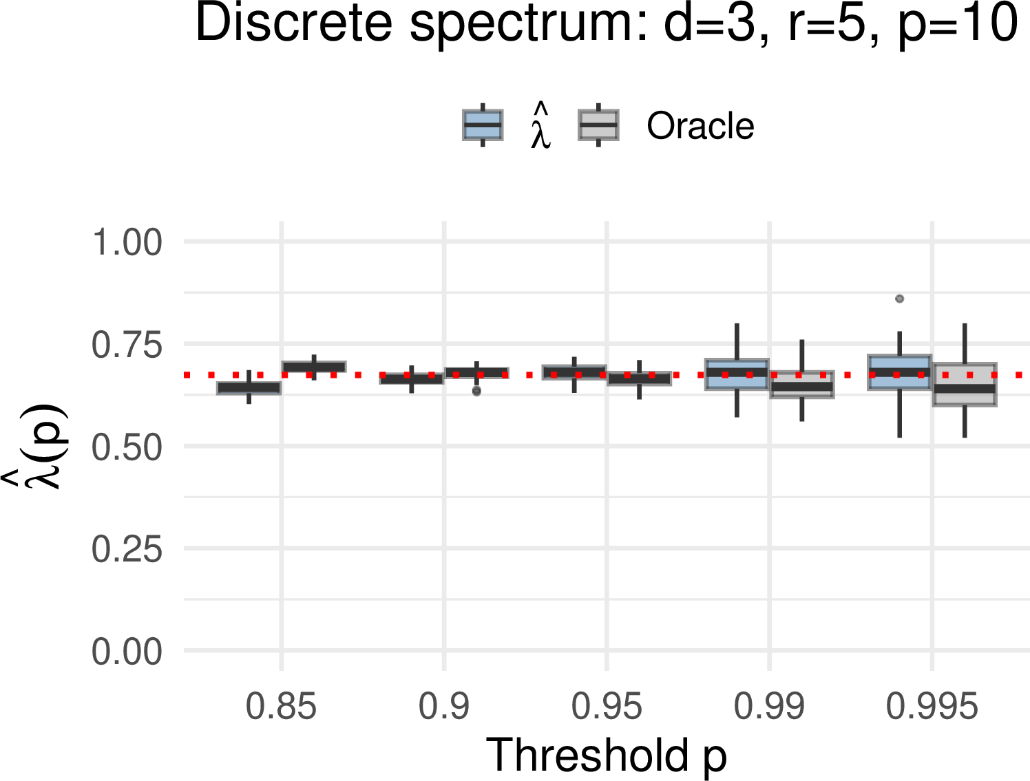
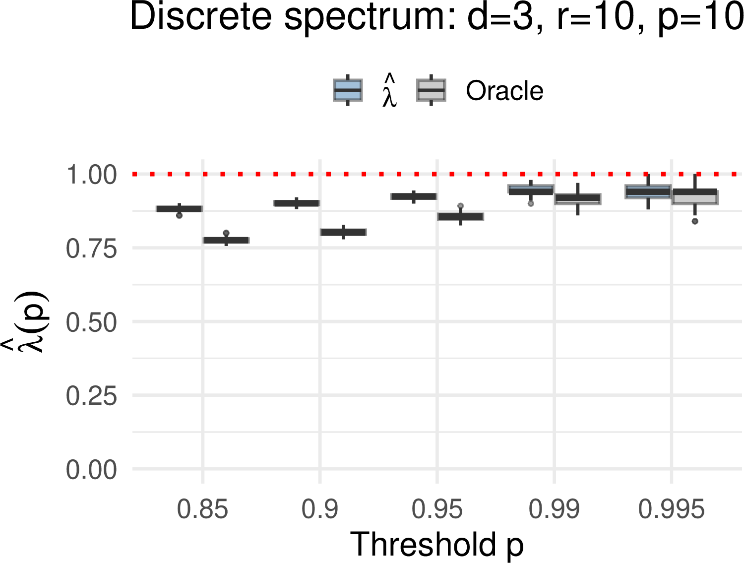
Figure 1: Pairs of boxplots of the empirical tail dependence coefficient \(\widehat {\lambda}(p)\) of the estimated predictor (left) and the oracle predictor (right) for several thresholds \(p \in\{0.85, 0.9, 0.95, 0.99, 0.995\}\), based on \(100\) independent replications of a spectrally discrete model. Left panel: Unobserved covariates present (\(r=5<p=10\)). Right panel: A perfect asymptotic precision scenario (\(r=p=10\)). The dotted red line marks the optimal asymptotic precision for the class of homogeneous predictors \(\lambda_{\cal H}^{\mathrm{opt}}\)..
Remark 19 (perfect asymptotic precision). Relation 74 reveals a remarkable perfect asymptotic precision* phenomenon. If all \(p\) latent factors contribute to \(X\) \((r=p)\) and no two directions \(\{a_i/\|a_i\|_1,\;i=1,\cdots,p\}\) coincide, then 74 implies \(\lambda^{(\mathrm{opt})}_{\mathcal{G}}(Y,X) = 1.\) This means that, asymptotically, one can predict the extremes of \(Y\) with perfect precision! This surprising phenomenon can be intuitively explained via the single large jump heuristic as follows. Conditionally on \(\{\|X\|_1>t\}\), as \(t\to\infty\), one and only one of the factors \(\xi_i\) will dominate in the sum 73 . Thus, the direction \(X/\|X\|_1\) identifies, asymptotically with probability one, the unique factor \(\xi_i\) responsible for the extreme event, which in turn determines \(Y\) exactly. For more details, see Section 9.1.*
Given the \(b_i\)’s and \(a_i\)’s, one can construct a continuous, non-negative, \(1\)-homogeneous function \(h^{(\mathrm{opt})}\) achieving 74 , which we refer to as the oracle predictor (see 137 ). In practice the \(b_i\)’s and \(a_i\)’s are unknown. Nevertheless, the spectral measure of \((Y,X)\) in 136 can be estimated consistently from data by using the peaks-over-threshold methodology combined with a non-parametric estimator of the quantiles of \(q_\alpha(\theta)\) the tilted conditional angular distribution (cf Algorithm 4).
Figure 1 illustrates the finite-sample behavior of our nonparametric estimator across repeated experiments: The left panel corresponds to the under-determined case \(r < p\), where 74 is strictly less than one, while the right panel shows the perfect precision case \(r = p\), where \(\lambda^{(\mathrm{opt})}_{\mathcal{G}} = 1\). The estimators are based on a training sample \(\{(Y_i,X_i)\}\) of \(n_{\rm train}= 10^4\) using a random threshold based on the \(0.95\)th empirical quantile. The empirical precision is then computed over an independently generated testing sample \(\{(Y_i^*,X_i^*)\}_{i=1}^{n_{\rm test}}\) of size \(n_{\rm test}=10^4\), where \[\label{e:wh-lambda40p41} \widehat \lambda(p):= \frac{1}{1-p} \sum_{i=1}^{n_{\rm test}} I\{ \widehat g(X_i^*) > \widehat F_{\widehat g}(p) \} I\{ Y_i^* > \widehat F_{Y}(p) \},\;\;p\in (0,1),\tag{75}\] where \(\widehat F_{\widehat g}\) and \(\widehat F_Y\) are the empirical CDFs of \(\{\widehat g(X_i^*)\}\) and \(\{Y_i^*\}\), respectively. The boxplots are based on \(100\) independent replications of the \(\widehat \lambda(p)\)’s. The coefficients \(b_i\) and the components of the vectors \(a_{i}\) in 73 were fixed across different replications, but drawn independently and at random from the Uniform\((0,1)\) distribution, therefore ensuring that \(a_i/\|a_i\| \not = a_j/\|a_j\|\), for all \(i\not = j\), with probability one.
Figure 1 shows a close agreement of the estimated optimal homogeneous predictor and the oracle, and both are rather close to the optimal homogeneous extremal precision (dashed horizontal line). It is remarkable
that the empirical tail dependence coefficient is nearly one for thresholds \(p\) as low as \(0.85\) in the asymptotically perfect precision scenario.
The Pareto-Dirichlet case. As an illustration of the spectrally continuous setting, consider \(Z = (Y,X) = \xi\cdot(V,W)\), where \(\xi\) is a standard \(1\)-Pareto random variable independent of \((V,W) \sim \mathrm{Dirichlet}(\beta)\) with parameter \(\beta = (\beta_0,\beta_1,\ldots,\beta_d) \in
(0,\infty)^{d+1}\). We call this the Pareto-Dirichlet\((\beta)\) model (cf Proposition 20). It is \(\tau\)-regularly varying with respect to the radial function \(\tau(y,x) = |y| + \|x\|_1\), and its angular measure is the Dirichlet distribution on the unit simplex \(\Delta_d\).
The neutrality property of the Dirichlet distribution [42] implies that \(U := V\) and \(\Theta := W/\|W\|_1\) are independent, so the conditional quantile \(q_\alpha(\theta)\) in Theorem 2 is constant in \(\theta\). This yields a remarkably simple optimal predictor (Proposition 20 in Section 9): \[\label{e:h-opt-Dirichlet-preview} h^{(\mathrm{opt})}(X) = c\,\|X\|_1, \qquad c := \frac{\beta_0}{\sum_{i=1}^{d}\beta_i},\tag{76}\] with optimal precision \[\label{e:lambda-opt-Dirichlet-preview} \lambda^{(\mathrm{opt})}_{\mathcal{G}}(Y,X) = \mathbb{E}\!\left[\frac{U}{\mu_U} \wedge \frac{1-U}{1-\mu_U}\right], \qquad U \sim \mathrm{Beta}\!\left(\beta_0,\,\textstyle\sum_{i=1}^d \beta_i\right), \quad \mu_U = \mathbb{E}[U].\tag{77}\] Moreover, \(\lambda^{(\mathrm{opt})}_{\mathcal{G}}(Y,X) = \lambda_p(Y, h^{(\mathrm{opt})}(X))\) for all \(p > p_0 := \mu_U \vee (1-\mu_U)\), so the precision is exactly constant beyond a threshold. This is clearly observed in the right panel of Figure 2, where the empirical tail-dependence coefficient \(\hat{\lambda}_p\) boxplots for both the oracle and the nonparametric estimator plateau at \(\lambda^{(\mathrm{opt})}_{\mathcal{G}}\) across a wide range of \(p\) values (see also Figure 3).
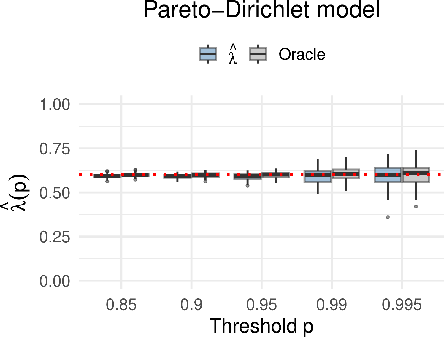
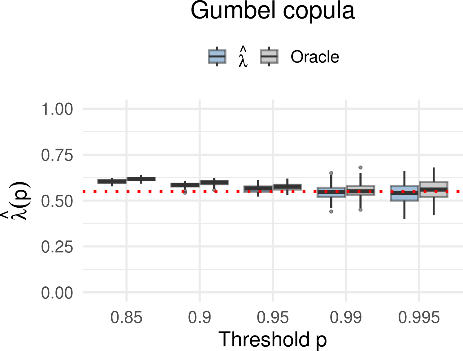
Figure 2: Pairs of boxplots of the empirical tail dependence coefficient \(\widehat {\lambda}(p)\) of the estimated predictor (left) and the oracle predictor (right) for several thresholds \(p\), based on \(100\) independent replications for two spectrally continuous models. Left panel: Pareto–Dirichlet spectral model (\(d=9\)). Right panel: Gumbel copula model (\(\beta=1.5\), \(d=10\)). The horizontal dotted red line marks the theoretically optimal asymptotic precision \(\lambda_{\cal H}^{\mathrm{opt}}\) in each case..
Figure 2 (left panel) shows boxplots of the empirical tail-dependence coefficients as in 75 based on \(100\) replications of an estimated optimal predictor and the corresponding oracle. As in Figure 1, we have \(n_{\rm train} = n_{\rm test} = 10^4\) and a random peaks-over-threshold of the \(0.95\)-th percentile. The Pareto-Dirichlet model involves coefficients \(\beta_0 = 1\) and \(\beta_i = (i+1)/10,\;i=1,\cdots,9\). As in the spectrally discrete case, we have a remarkably close agreement in the precision of the estimated predictor and the oracle, which in this case is simply proportional to \(\|X\|_1\). Both agree closely with the asymptotically optimal precision as indicated above.
The right panel of Figure 2 shows the same type of experiment where \((Y,X)\) come from a Gumbel copula, where \(d=10\). By Corollary 2, in this case the optimal homogeneous predictor is in fact the ultimate optimal predictor for all values of \(p\in (0,1)\). In this scenario, the non-parametric estimator is remarkably close to the oracle.
These brief simulation results illustrate the success of the optimal homogeneous prediction methodology. The quantile regression forest based implementation is nearly tuning–free and quite adaptive – working well in both spectrally discrete and continuous settings. We have implemented this methodology in the context of the challenging open problem of Solar flare prediction, where we found it to work out-of-the-box and provide state-of-the-art prediction scores for the most extreme X-class flares (cf Figure 6). We plan to pursue more applied and methodological directions of this research in a future work, but the preliminary findings are available in Section 11. The code used to produce all simulation in the paper is freely available from the GitHub repository [18]. An R Shiny app illustrating the methodology over a challenging Solar flare prediction problem is deployed on [19].
6 Discussion and future work↩︎
In this paper, we considered the fundamental problem of optimal extreme event prediction in terms of covariates. Starting from a general the Neyman-Pearson-type characterization of the optimal predictors (Theorem 1), we formulated an optimality framework that is closely related to the notion of tail-dependence. This naturally led us to explore the problem of optimal extremal prediction in the context of jointly regularly varying response and covariates. For the general class where the predictors are positive homogeneous of the covariates, the problem was cast into a variational problem – a constrained optimization problem for a convex integral functional with respect to the angular measure. Our first main contribution was an explicit solution to this problem (Theorem 2), which can be represented in terms of the quantiles of a certain tilted conditional distribution arising from the angular measure. This abstract result let us to concrete and yet general inference methodology for the optimal homogeneous predictors. Our second contribution was to establish the consistency for estimators of these optimal predictors in the framework of peaks-over-threshold (Theorem 3). This result, modulo mild regularity conditions, may be viewed as an extremal counterpart to the celebrated Stone’s Universal Consistency Theorems for the class of homogeneous predictors. Last but not least, using established quantile regression forests tools, the estimators were implemented into a broadly applicable and nearly tuning free statistical software, which was shown to achieve the oracle performance over simulated examples.
The problem of extreme event prediction is fundamental and ubiquitous. It can be seen as a series of increasingly imbalanced classification problems, which is rather challenging. Notably, [9] have identified the shortcomings of the traditional empirical risk minimization approach and proposed a solution. While motivated by similar problems, our approach is different. Here, by conditioning on the regime of extremes, the loss function is directly related to tail-dependence, which allowed us to take a different look through the lens of calculus of variations.
We provide a rather complete solution to the optimal extremal prediction with homogeneous functions in the context of jointly regularly varying \(Y\) and \(X\). While in many cases the class of homogeneous predictors do contain the optimal extremal predictors (cf Example 1 and Corollary 2), this is not always the case. Indeed, as shown in Example 8, even under joint regular variation, the ‘extremes’ of \(X\) do not necessarily predict the extremes of \(Y\). To the best of our knowledge, the problem of finding universally consistent predictors in the extreme value sense, remains open both in terms of its precise formulation and solution.
Acknowledgments↩︎
We thank Victor Verma for providing curated the GOES flux time series and SHARP parameter data for the Solar flare prediction experiment in Section 11. SS was partially supported by the NSF grant CNS/CSE-2319592 “Collaborative Research: IMR: MM-1A: Scalable Statistical Methodology for Performance Monitoring, Anomaly Identification, and Mapping Network Accessibility from Active Measurements”.
7 Examples↩︎
7.1 Examples of optimal predictors↩︎
In this section, we elaborate on the closed-form optimal predictors discussed in Section 2. Specifically, we prove the stated characterizations of the optimal predictors in the bi-variate max-stable and Archimedean copula models with completely monotone generators.
7.1.1 Bivariate extreme value distributions↩︎
Suppose that \((Y,X)\) follow the a bivariate extreme value distribution \(G\), where without loss of generality the marginal distributions of \(X\) and \(Y\) are standard unit Fréchet. That is, \[F_X(u) = \mathbb{P}[X\le u] = F_Y(u) = \mathbb{P}[Y\le u] = \exp\{-1/u\},\;u>0.\] It is known that [35], for all \(x,y\ge 0,\) \[\label{e:G-EVD} G(x,y) = e^{-\mu(A_{x,y})},\tag{78}\] where \(A_{x,y} = [0,\infty)^2 \setminus ([0,x]\times[0,y])\) and \(\mu\) is a Borel measure on \([0,\infty)^2\setminus \{(0,0)\}\), such that \(\mu(A_{x,y})<\infty\) provided \(x>0\) or \(y>0\). It can be shown that \(\mu(t A) = t^{-1} \mu(A)\), for all \(t>0\) and Borel sets \(A\subset [0,\infty)^2\setminus \{(0,0)\}\) and hence for all \(x,y \ge 0\) \[\label{e:G-EVD-spectral} G(x,y) = \exp\Big\{ - V(1/x,1/y) \Big\},\;\; where V(a,b):= \int_0^1 \max\{ w a, (1-w) b)\} \sigma(dw)\tag{79}\] where \(\sigma\) is a finite measure on \([0,1]\) and by convention \(1/\infty = 0\) and \(1/0 = \infty\). The function \(V\) is referred to as the stable tail-dependence function of the bivariate extreme value distribution.
The following result is rather natural and it shows that the events \(\{X>x_0\}\) are optimal predictors of \(\{Y>y_0\}\).
Proposition 10. Let \((X,Y)\) be a bivariate max-stable random vector with joint distribution function \(G\) as in 78 . Suppose that \(G(x,y)\) is continuously differentiable in \(x\) and \(y\), so that \(g(x,y):= \partial^2_{x,y}G(x,y)\) is the joint density of \((X,Y)\) with respect to the Lebesgue measure. Then, for all \(y_0>0\), the predictor \(\{X> F_X^{-1}(q)\}\) is an optimal predictor of \(\{Y>y_0\}\), calibrated at level \(q\).
Proof. In view of Theorem 1, an optimal predictor of \(\{Y>y_0\}\) is of the form \(\{r(X)>\tau\}\), where \(r(x) = f_0(x)/f_1(x)\), where \(f_0\) and \(f_1\) are the conditional densities of \(X|\{Y>y_0\}\) and \(X|\{Y\le y_0\}\), respectively. Let \(p:= \mathbb{P}[ Y>y_0]\) and observe that for all \(x>0\): \[f_0(x) = \frac{1}{1-p} \int_{y_0}^\infty g(x,y) dy = \frac{1}{1-p} \Big( \partial_x G(x,\infty) - \partial_x G(x,y_0) \Big)\] Similarly, \[f_1(x) = \frac{1}{p} \int_{0}^{y_0} g(x,y) dy = \frac{1}{p} \Big( \partial_x G(x,y_0) - \partial_x G(x,0) \Big) = \frac{1}{p} \partial_x G(x,y_0),\] where we used that \(\partial_x G(x,0) = 0\).
This shows that \[r(x) = \frac{f_0(x)}{f_1(x)} = \frac{p}{(1-p)}\cdot \frac{\partial_x G(x,\infty)}{ \partial_x G(x,y_0)} - \frac{p}{1-p}.\] We will show that the function \[\label{e:p:max-stable-0} x\mapsto \frac{\partial_x G(x,\infty)}{ \partial_x G(x,y_0)}\tag{80}\] is increasing in \(x\). This would complete the proof since it will show that the events \(\{r(X)>\tau\}\) and \(\{ X> \tau'\}\) are the same, when calibrated at the same level \(q\).
To this end, since \(G(x,y) = \exp\{ -V(1/x,1/y)\}\), by the chain rule, we obtain \[\partial_x G(x,y) = x^{-2} \partial_a V(1/x,1/y) e^{-V(1/x,1/y)}.\] Note, however, \(\partial_a V(a,0) = 1\) since \(V(a,0) = a\). Thus, \(\partial_x G(x,\infty) = x^{-2} \exp\{ -V(1/x,0)\}\) and \[\begin{align} \label{e:p:max-stable-1} \frac{\partial_x G(x,\infty)}{ \partial_x G(x,y_0)} = \frac{\exp\{ V(1/x,1/y_0) - V(1/x,0)\}}{\partial_a V(1/x,1/y_0)} = \frac{\exp\{ \mu(A_{x,y_0}) - \mu(A_{x,\infty}) \}}{\partial_a V(1/x,1/y_0)}, \end{align}\tag{81}\] where we used the fact that \(V(1/x,1/y) = \mu(A_{x,y})\) with \(A_{x,y} = [0,\infty)^2 \setminus ([0,x]\times [0,y]),\;x,y\in (0,\infty)\), and \(A_{x,\infty} = [0,\infty)^2 \setminus ([0,x]\times [0,\infty])\).
Now, for the numerator in the right-hand side of 81 , we obtain \[\exp\{ \mu(A_{x,y}) - \mu(A_{x,\infty}) \} = \exp\{ \mu( [0,x]\times (y_0,\infty) ) \},\] which is a monotone increasing function of \(x\) since the sets \([0,x] \times (y_0,\infty)\) grow as \(x\) grows. On the other hand, \(a\mapsto \partial_a V(a,b)\) is a monotone non-decreasing function of \(a\). Indeed, in view of 79 , we have that \(a\mapsto V(a,b)\) is a convex function, and therefore its partial derivative is non-decreasing in \(a\). This implies that the denominator \(x \mapsto \partial_a V(1/x,1/y_0)\) in the right-hand side of 81 is a monotone non-increasing function of \(x.\) This, combined with the established monotonously of the numerator implies that the function in 80 is monotone non-decreasing in \(x\), which completes the proof of the proposition. ◻
Remark 20. Let \((Y,X)\) be as in Proposition 10. This result implies the optimal extremal precision \(\lambda^{\rm(opt)}(Y,X)\) equals the tail-dependence coefficient \(\lambda(Y,X)\) (see also Example 6).
7.1.2 Archimedean copula: Proofs for Section 2.2↩︎
We start with the following auxiliary result.
Lemma 7. The positive completely monotone functions are log-convex.
Proof. Let \(\psi\) be as in 4 . Recall that the function \(\psi:(0,\infty)\to (0,\infty)\) is log-convex if \(\log(\psi(\cdot))\) is convex, or, equivalently: \[\begin{align} \label{e:l:Bernstein-log-convex-0} \psi(\lambda u + (1-\lambda)v) \le \psi(u)^\lambda \psi(v)^{1-\lambda}, \end{align}\tag{82}\] for all \(u,v >0\) and \(\lambda \in (0,1)\). In view of 4 , for all \(\lambda \in (0,1)\), \[\begin{align} \label{e:l:Bernstein-log-convex} \psi(\lambda u + (1-\lambda)v) &= \int_0^\infty e^{- \lambda ux } e^{-(1-\lambda)vx} \mu(dx)\nonumber\\ & \le \Big(\int_0^\infty e^{- ux }\mu(dx)\Big)^{1/p} \Big(\int_0^\infty e^{- vx }\mu(dx)\Big)^{1/q}, \end{align}\tag{83}\] where the last bound follows from the Hölder inequality applied to the functions \(f(x):=e^{-\lambda ux}\in L^p(\mu(dx))\) and \(g(x):= e^{-(1-\lambda)vx} \in L^q(\mu(dx))\), with \(p:=1/\lambda\) and \(q:=1/(1-\lambda)\). This completes the proof since the right-hand sides of 82 and 83 are the same. ◻
Proposition 11 (Statement of Proposition 1). Let \((Y,X_1,\cdots,X_d)\) be a random vector in \(\mathbb{R}^{1+d}\) with continuous marginal cdfs \(F_Y\) and \(F_{X_i},\;i=1,\cdots,d\), respectively, and the Archimedean copula \(C\) as in 3 , where \(\psi\) is a completely monotone function as in 4 . Then, for all \(\tau>0\), the events \[\Big\{ \psi \Big( \psi^{-1}(F_{X_1}(X_1))+\cdots + \psi^{-1}(F_{X_d}(X_d)) \Big) > \tau \Big\}\] are optimal predictors of the events \(\{Y>y_0\}\) in terms of \(X\).
Proof of Proposition 1.. Without loss of generality, assume that the marginals of \((Y,X)\) are uniform, i.e., the joint cdf of \((Y,X)\) is the copula \(C\) in 3 . Let for convenience \(\varphi(t):=\psi^{-1}(t)\) and observe that the joint density of \((X,Y)\) with respect to the Lebesgue measure is: \[f_{Y,X}(y,x) = \partial_{y,x}^{d+1}C(y,x) = \psi^{(d+1)}\Big(\varphi(y)+\varphi(x_1)+\cdots+\varphi(x_d) \Big) \varphi'(y) \prod_{i=1}^d \varphi'(x_i),\] where \(x =(x_i)_{i=1}^d \in (0,1)^d,\;y\in (0,1)\). Therefore, with \(p:= \mathbb{P}[Y >y_0] \in (0,1)\), for the conditional densities \(f_0\) and \(f_1\) of \(X|\{Y>y_0\}\) and \(X|\{Y\le y_0\}\) in Theorem 1, we obtain \[\begin{align} \label{p:archimedean-1} f_0(x) & = \frac{\prod_{i=1}^d \varphi'(x_i)}{(1-p)} \int_{y_0}^1 \psi^{(d+1)}(\varphi(x_1)+\cdots+\varphi(x_d) + \varphi(y)) \varphi'(y) dy\nonumber \\ & = \frac{\prod_{i=1}^d \varphi'(x_i)}{(1-p)} \int_{y_0}^1 h'( c + \varphi(y)) \varphi'(y) dy, \end{align}\tag{84}\] where for clarity, we let \(h(t):= \psi^{(d)}(t)\) and \(c:= \varphi(x_1)+\cdots+\varphi(x_d)\). The fundamental theorem of calculus applied to the integral in the right-hand side of 84 then implies \[\begin{align} \label{e:p:archimedean-f0} f_0(x) & = \frac{\prod_{i=1}^d \varphi'(x_i)}{(1-p)} \Big( h(c) - h(c+\varphi(y_0))\Big), \end{align}\tag{85}\] where we used that \(\varphi(1) = 0\). Similarly, for \(f_1\), we obtain \[\begin{align} \label{e:p:archimedean-f1} f_1(x) & = \frac{\prod_{i=1}^d \varphi'(x_i)}{p} \int_{0}^{y_0} h'( c + \varphi(y)) \varphi'(y) dy \nonumber\\ & = \frac{\prod_{i=1}^d \varphi'(x_i)}{p} \Big(h(c+\varphi(y_0)) - h(\infty)\Big), \end{align}\tag{86}\] where we used that \(\varphi(0) = \infty.\) In view of 4 , we have \[h(u) = \psi^{(d)}(u) = (-1)^d \int_0^\infty e^{-ux} x^d \mu(dx)\] and hence \(h(\infty) = \lim_{u\to\infty} h(u) = 0\). Thus, for the ratio \(r(x) = f_0(x)/f_1(x)\), in view of 85 and 86 , we obtain: \[\label{e:p:archimedean-r} r(x) = \frac{f_0(x)}{f_1(x)} \propto \frac{\psi^{(d)}( c )}{ \psi^{(d)}( c + \varphi(y_0))} -1,\tag{87}\] where recall that \(c = c(x) := \psi^{-1}(x_1) +\cdots+\psi^{-1}(x_d)\). In view of Theorem 1, the events \(\{r(X)>\tau\}\) are optimal predictors of \(\{Y>y_0\}\). Thus, in view of 87 , to complete the proof it is enough to establish that the function \[c := \frac{\psi^{(d)}( c )}{ \psi^{(d)}( \varphi(y_0)+c )}\] is decreasing in \(c\). We will show that this is the case by using the log-convexity of the positive completely monotone functions (Lemma 7).
Indeed, observe that \[g(c)= \frac{\psi_d ( c )}{ \psi_d( \varphi(y_0) + c )},\] where \(\psi_d(u) := (-1)^d \psi^{(d)}(u) = \int_0^\infty e^{-ux} x^d \mu(dx).\) Notice that the function \(\psi_d\) is also completely monotone and hence it is log-convex.
We have that \[\label{e:p:archimedean-1} \frac{d}{dc}\log( g (c)) = \frac{\psi_d'(c)}{\psi_d(c)} - \frac{\psi_d'( \varphi(y_0)+c)}{\psi_d( \varphi(y_0)+c)}.\tag{88}\] Since \(\psi_d\) is log-convex, we have that \[c\mapsto \frac{\psi_d'(c)}{\psi_d(c)} = \frac{d}{dc}\log(\psi_d(c))\] is an increasing function. Since \(\varphi(y_0)\ge 0\), this implies that the right-hand side of 88 is non-positive, \(d/dc ( \log(g(c)) \le 0\) and this establishes that the function \(c\mapsto g(c)\) is decreasing and the proof is complete. ◻
Proposition 1 implies the following result, which is of independent interest since it concerns an important class of multivariate max-stable models.
Corollary 2. Assume that \((Y,X)\) follow the multivariate logistic max-stable distribution in ?? , with parameter \(\beta>1\). Then, for all \(p,q\in (0,1)\), an optimal predictor of \(\{Y>F_Y^{-1}(p)\}\) is of the form: \[\{h(X) > F_{h(X)}^{-1}(q)\},\;\; where \;h(X) =\Big(\sum_{i=1}^d \frac{1}{X_i^\beta} \Big)^{-1/\beta}.\]
Moreover, the optimal extremal precision is given by: \[\label{e:c:logistic} \lambda^{\rm (opt)}(Y,X) = \lambda(Y,h(X)) = \mathbb{E}\Big[ \min\Big\{ \Gamma_1^{-1/\beta}/c_{1,\beta},\;\Gamma_d^{-1/\beta}/c_{d,\beta} \Big\} \Big],\qquad{(27)}\] where \(\Gamma_1\sim {\rm Gamma}(1,1)\) and \(\Gamma_d \sim {\rm Gamma}(d,1)\) are independent Gamma-distributed random variables and where \(c_{d,\beta} = \Gamma(d-1/\beta)/\Gamma(d)\).
Proof of Corollary 2. Let \(\beta >1\) and \(Z\) a \(1/\beta\)-stable subordinator. That is, a positive random variable with the Laplace transform \[\psi_Z(t) = \mathbb{E}[ e^{-tZ} ] = e^{-t^{1/\beta}},\;t\ge 0.\] Let also \(\xi_i,\;i=1,\cdots,d\) and \(\eta\) be independent standard \(\beta-\)Fréchet random variables, i.e., such that \[\mathbb{P}[\xi_i\le x] = \mathbb{P}[\eta \le x] = e^{-x^{-\beta}},\;x>0.\] Assume that \(Z\) and \(\xi = (\xi_i)_{i=1}^d\) and \(\eta\) are independent. Then, the multivariate logistic max-stable random vector \((X,Y)\) in ?? has the following stochastic representation: \[(X,Y) = Z^{1/\beta}\cdot( \xi,\eta),\] where \(\xi = (\xi_i)_{i=1}^d\) (see e.g., [43]).
Proposition 1 shows that the optimal predictor of \(\{Y>y_0\}\) is of the form \(\{\|1/X\|_\beta^{-1}>\tau\}\), where \(\|1/X\|_\beta:= (\sum_{i=1}^d X_i^{-\beta})^{1/\beta}\). We will derive next the optimal extremal precision \[\lambda^{\rm (opt)}(Y,X) = \lambda (Y, 1/\|1/X\|_\beta).\] We have that \(1/\eta^\beta\) and \(1/\xi_i^\beta =:E_i \sim {\rm Exponential}(1)\) are standard Exponentially distributed. Therefore, \[1/\|1/X\|_\beta = Z^{1/\beta} \Big(\sum_{i=1}^d E_i\Big)^{-1/\beta} =: Z^{1/\beta} \frac{1}{\Gamma_d^{1/\beta}},\] where \(\Gamma_d = E_1+\cdots+E_d\sim{\rm Gamma}(d,1)\). Similarly, \[Y = Z^{1/\beta} \eta =: Z^{1/\beta} \frac{1}{\Gamma_1^{1/\beta}},\] where \(\Gamma_1:= \eta^{-\beta}\sim {\rm Gamma}(1,1)\).
Now, we have that \[\mathbb{P}[Z^{1/\beta}>x] \sim c_\beta^{-1} \frac{1}{x}, \;\; as x\to\infty,\] where in fact \(c_\beta = \Gamma(1-1/\beta)\) [44]. Therefore, by Breiman’s Lemma, we have \[\mathbb{P}[Y>x] = \mathbb{P}[Z^{1/\beta} \eta > x] \sim c_\beta^{-1} \frac{\mathbb{E}[\eta] }{x} = \frac{1}{x},\;\;x\to\infty,\] since \(\mathbb{E}[\eta] = \int_0^\infty x^{1} d e^{-x^{-\beta}}=\Gamma(1-1/\beta) = c_\beta\). By Breiman’s lemma, we also have \[\mathbb{P}[1/\|1/X\|_\beta > x] = \mathbb{P}[ Z^{1/\beta} \Gamma_d^{-1/\beta}>x] \sim c_\beta^{-1} \mathbb{E}[\Gamma_d^{-1/\beta}] \frac{1}{x} = \frac{\Gamma(d-1/\beta)}{\Gamma(d)c_\beta} \frac{1}{x} =: \sigma_{d,\beta} \frac{1}{x}.\] Thus, the random variable \(\|1/X\|_\beta^{-1}/\sigma_{d,\beta}\) has unit asymptotic scale, i.e., it is asymptotically calibrated: \[\mathbb{P}[\|1/X\|_\beta^{-1}/\sigma_{d,\beta} > x ] \sim \mathbb{P}[Y> x] \sim \frac{1}{x},\;\;x\to\infty.\] This, implies that \[\mathbb{P}[ \|1/X\|_\beta^{-1}/\sigma_{d,\beta} \wedge Y > x] \sim \lambda(Y, \|1/X\|_\beta^{-1}) \frac{1}{x} = c_\beta^{-1} \mathbb{E}[ \Gamma_d^{-1/\beta}/\sigma_{d,\beta} \wedge \Gamma_1^{-1/\beta}] \frac{1}{x},\] by another application of Breiman’s lemma. Therefore, observing that \(c_\beta = c_{1,\beta} = \Gamma(1-1/\beta)\) and \(c_\beta \sigma_{d,\beta} = \Gamma(d-1/\beta)/\Gamma(d),\;d=1,2,\ldots\), we obtain ?? . ◻
8 Proofs↩︎
8.1 Multivariate regular variation↩︎
In this section, we provide a brief review of the theory of multivariate regular variation of Borel measures on \(\mathbb{R}^k,\;k\ge 1\). We consider the general case of \(\tau\)-regular variation, where \[\label{e:tau} \tau:\mathbb{R}^k \to \mathbb{R}_+\tag{89}\] is a fixed non-negative, continuous \(1\)-homogeneous function [26], [27]. For an abstract and general theory of regular variation with respect to the notion of a bornology, see e.g., [28] and the references therein.
8.2 The space \(\mathbb{M}_\tau\) and the Tail Index Theorem↩︎
Let \(\mathbb{M}_\tau = \{ \mu\, :\, \mu(\tau >\epsilon)<\infty,\; for all \epsilon>0\}\) be the collection of Borel measures \(\mu\) on \(\mathbb{R}^k\setminus\{\tau=0\}\) such that \(\mu(\{\tau>\epsilon\})<\infty\), for all \(\epsilon>0\). Such measures assign finite masses to all Borel sets \(A\) that are bounded away from \(0\), relative to the \(\tau\)-loss, i.e., \(\tau(A):=\inf_{x\in A}\tau(x)\) is positive. We shall denote this class of Borel sets by \({\cal B}_0(\tau)\) and \({\cal B}(\tau) = \sigma({\cal B}_0(\tau))\) is the \(\sigma\)-field of all Borel sets in \(\mathbb{R}^k\setminus\{\tau=0\}\).
If \(\mu_n,\mu\in \mathbb{M}_\tau\), then we write \(\mu_n\stackrel{M_0}{\to} \mu\), as \(n\to\infty\), if \[\label{e:M0-convergence-via-f} \int f(x)\mu_n(dx) \to \int f(x)\mu(dx),\;\; as n\to\infty,\tag{90}\] for all bounded and continuous functions \(f\) such that \(\{|f|>0\} \subset \{\tau>\epsilon\}\) for some \(\epsilon>0\). It can be shown that \(\mu_n\stackrel{M_0}{\to} \mu\) if and only if \[\mu_n(A)\to \mu(A),\;\; as n\to\infty,\] for all \(A\in {\cal B}_0(\tau)\) such that \(\mu(\partial A) =0\), where \(\partial A:=\overline{A}\setminus A^\circ\) denotes the topological boundary of the set \(A\) [45]. The above-defined \(M_0\)-convergence of measures in \(\mathbb{M}_\tau\) is generated by a metric, which renders \(\mathbb{M}_\tau\) a complete separable metric space [45].
Definition 6. Let \(\tau\) be a fixed continuous \(1\)-homogeneous function as in 89 . Consider a random vector \(Z\) in \(\mathbb{R}^k,\;k\ge 1\). If there is a positive sequence \(\{a_n\}\) and a non-zero measure \(\mu \in \mathbb{M}_\tau\) such that \[\mu_n:= n \mathbb{P}[Z/a_n\in \cdot] \stackrel{M_0}{\to} \mu,\;\; as n\to\infty,\] then we say that \(Z\) is \(\tau\)-regularly varying and write \(Z\in RV(\{a_n\},\mu)\).
Theorem 4 (The tail index theorem). If \(Z\in RV(\{a_n\},\mu)\) according to Definition 6, then:
There exists a positive \(\alpha>0\) such that \(a_n \sim \ell(n) n^{1/\alpha}\), for some slowly varying function \(\ell(\cdot)\).
The measure \(\mu\) satisfies the scaling relation: \[\label{e:thm:tail-index:scaling} \mu(t\cdot A) = t^{-\alpha} \mu(A),\;\; for all t>0 and A\in {\cal B}(\tau).\qquad{(28)}\]
If also \(Z\in RV(\{b_n\},\nu)\), then \[\frac{a_n}{b_n} \to c \in (0,\infty),\;\; and \;\;\mu(A) = c^{-\alpha} \nu(A),\; for all A\in {\cal B}(\tau).\] Consequently, the parameter \(\alpha>0\), referred to as the tail exponent of \(Z\) is unique, and so is the measure \(\mu\), up to a rescaling factor.
We have that \(Z\in {\rm RV}_\alpha(\mathbb{R}^k,\{a_n\},\;c_Z, \tau, \sigma)\) according to Definition 4, where \[c_Z:= \mu(\{\tau>1\}) \;\; and\;\; \sigma(B) := \frac{1}{\mu(\{\tau>1\})} \mu(\{ x/\tau(x) \in B\}),\;\;B\in {\cal B}(S_\tau).\]
Conversely, if \(Z\in {\rm RV}_\alpha(\mathbb{R}^k,\{a_n\},\;c_Z, \tau, \sigma)\) according to Definition 4, then \(Z\in RV_\alpha(\{a_n\},\mu)\) according to Definition 6, where \[\label{e:thm:tail-index:disintegration} \mu\circ T_\tau^{-1}( (r,\infty)\times B) ) = c_Z r^{-\alpha} \sigma(B),\;\; for allr>0,\;B\in {\cal B}(S_\tau),\qquad{(29)}\] and where \(T_\tau : \mathbb{R}^k\setminus\{\tau=0\} \to (0,\infty)\times S_\tau\) is the generalized polar coordinated homeomorphism defined as \(T_\tau(x) = (\tau(x), x/\tau(x))\).
The proof of this result can be derived from many excellent treatments in the literature. Specifically, see, for example, Theorem 3.1 and Corollary 4.4 in [46], as well as [45], [47], the monographs [25], [29], the general theory in [28], and the references therein for more details.
8.3 Proofs for Section 3↩︎
8.3.1 Proofs for Section 3.1↩︎
For completeness, we will present the proof of Proposition 2 below although similar results can be found in Proposition 2.5 of [23] and Theorem 2.1 of [30]. The proof consequence of the following characterization of multivariate regular variation [25].
Proposition 12. We have \(Z \in RV_\alpha(\mathbb{R}^k,\{a_n\},c_Z, \tau,\sigma)\) if and only if \[\label{e:p:rv-via-Pareto-Theta} \Big( \frac{\tau(Z)}{t}, \frac{Z}{\tau(Z)} \Big) \Big\vert \tau(Z)>t \stackrel{d}{\longrightarrow} (V, \Theta), \;\;(t\to\infty),\qquad{(30)}\] where \(V\) and \(\Theta\) are independent and \(\mathbb{P}[V>x]= x^{-\alpha},\;x\ge 1\), while \(\Theta\sim \sigma\).
Proposition 13 (Statement of Proposition 2). Let \(Z \in RV_\alpha(\mathbb{R}^k,\{a_n\},b(\cdot),c_Z,\tau,\sigma)\). Let also \({\cal H}_+(\mathbb{R}^k,\tau)\) denote the class of all non-negative continuous \(1\)-homogeneous functions \(h:\mathbb{R}^d\to \mathbb{R}_+\) such that \(\{h>0\} \subset \{\tau>0\}\). Then, for all \(h\in {\cal H}_+(\mathbb{R}^k,\tau)\), such that \[\label{e:p:rv-via-h-assumption-A} \|h\|_{\infty,S_\tau} := \sup_{\theta \in S_\tau} |h(\theta)| <\infty,\qquad{(31)}\] we have \[\label{e:p:rv-via-h-A} \lim_{n\to\infty} n\mathbb{P}[ h(Z) > a_n ] = \lim_{t\to\infty} b(t)\mathbb{P}[ h(Z) > t ] = c_Z \sigma(h),\qquad{(32)}\] where \[\sigma(h) := \mathbb{E}[h(\Theta_Z)^\alpha] = \int_{S_\tau} h^\alpha(\theta) \sigma(d\theta).\]
Proof of Proposition 2. Without loss of generality suppose that the positive normalizing sequence \(\{a_n\}\) is such that \(c_Z=1\). Observe that by the support domination condition \(\{h>0\} \subset \{\tau>0\}\), we have \(\{h(Z)>a_n\}\) implies \(\{\tau(Z)>0\}\). Also, note that since by ?? , \(h\) is bounded on the set \(S_\tau\), we have \[\tau(Z) h(Z/\tau(Z)) >a_n \;\; implies \;\;\tau(Z)>a_n/\|h\|_{\infty,S_\tau},\] where \(\|h\|_{\infty,S_\tau}\) is as in ?? .
Note that in the case \(\|h\|_{\infty,S_\tau}=0\), the result trivially holds. On the other hand for \(c_h:= \|h\|_{\infty,S_\tau}>0\), we have \[\mathbb{P}[ h(Z)>a_n] = \mathbb{P}[\tau(Z) h(Z/\tau(Z)) > a_n, \tau(Z) > a_n/c_h].\] Hence, using that \(n\mathbb{P}[\tau(Z)> t a_n]\to t^{-\alpha}\) \[\begin{align} \label{e:e:p:rv-via-Pareto-Theta-1} n \mathbb{P}[ h(Z)>a_n] &= n \mathbb{P}[\tau(Z)>a_n/c_h] \cdot \mathbb{P}\Big[ \frac{\tau(Z)}{a_n/c_h}\cdot h\Big( \frac{Z}{\tau(Z)} \Big) > c_h \Big\vert \tau(Z)>a_n/c_h \Big]\nonumber\\ & \longrightarrow c_h^\alpha \cdot \mathbb{P}[ V h(\Theta) > c_h ],\;\;(a_n\to\infty) \end{align}\tag{91}\] where the last convergence follows from ?? and the fact that \(V h(\Theta)\) is a continuous random variable.
It remains to observe that by the independence of \(V\) and \(\Theta_Z:=\Theta\), we have \[\mathbb{P}\Big[ V h(\Theta_Z) > c_h \Big] = \mathbb{E}[ I(V> c_h/h(\Theta_Z)] =\mathbb{E}\Big[ \Big(c_h/h(\Theta_Z)\Big)^{-\alpha}\Big] = c_h^{-\alpha} \mathbb{E}[ h(\Theta_Z)^\alpha].\] By combining this calculation with Relation 91 , we obtain that the first limit in ?? equals \(c_Z\mathbb{E}[h^\alpha(\Theta_Z)]\). The fact that the two limits in ?? coincide follows from the equivalence \(b(a_n)\sim n\) as \(n\to\infty\), which completes the proof. ◻
Lemma 8 (Statement of Lemma 1). Let \((Y,X)\) and \({\cal G}(\tau_X)\) be as in Definition 5. Then, for all \(g\in {\cal G}(\tau_X)\) the bivariate tail dependence coefficient \(\lambda(Y,g(X))\) defined in 7 exists and \[\label{e:lem:nonameidea-restatement} \lambda(g(X),Y) = \lim_{t\uparrow \infty} \mathbb{P}[ Y > t | g(X) > t ] = \lim_{t\uparrow \infty} \mathbb{P}[ g(X) > t | Y > t ].\qquad{(33)}\]
Proof of Lemma 1. By the transfer of regular variation theorem [25], we have \((\xi,\eta) := (g(X),Y)\) is regularly varying with exponent measure \(\nu := \mu\circ T_g^{-1}\), where \(T_g(y,x):= (g(x),y)\). More precisely, \[n \mathbb{P}[ (\xi,\eta) \in a_n A] \to \nu(A),\;\; as n\to\infty,\] for all Borel \(\nu\)-continuity sets. Equivalently [25], \[\label{e:lem:nonameidea-RV-via-b} b(t) \mathbb{P}[ (\xi,\eta) \in t\cdot A] \to \nu(A),\;\; as t\to\infty,\tag{92}\] for a suitable function \(b(\cdot)\), which is regularly varying at infinity with exponent \(1\).
The calibration property implies that \[\label{e:tail-equivalence-xi-eta} \mathbb{P}[\xi>t]\sim \mathbb{P}[\eta>t],\;\; as t\to\infty.\tag{93}\] Thus, by Lemma 9, since \(\xi\) and \(\eta\) have regularly varying right tails, to prove the result, it is enough to show that \[\label{e:lem:nonameidea-lambda-via-nu} \lim_{t\to\infty} \mathbb{P}[\xi>t | \eta>t] = \lim_{t\to\infty} \mathbb{P}[\eta>t | \xi>t] = \frac{\nu(A_1\cap A_2)}{\nu(A_1)},\tag{94}\] where \(A_i= \{ (u_1,u_2)\in \mathbb{R}^2\, :\, u_i\ge 1\}\).
To establish 94 , observe that for all \(t,s>0\), the sets \(A_{(t,s)}:= [t,\infty)\times [s,\infty)\) are \(\nu\)-continuity sets. Indeed, this follows from the homogeneity of the measure \(\nu\). For all \(t,s>0\) and \(\epsilon\in (0,1)\), we have that \(A_{\epsilon\cdot(t,s)} = \cup_{u \in [\epsilon,\infty)} \partial A_{u\cdot(t,s)}\), where the latter is a union of pairwise disjoint sets indexed by \(u\). This, since \(\nu(A_{\epsilon\cdot(t,s)})<\infty\), implies that all but countably many of the terms \(\nu(\partial A_{u\cdot(t,s)})\) vanish. Notice, however, that by the homogeneity of \(\nu\), since \(\partial A_{u\cdot(t,s)} = u\cdot \partial A_{(t,s)}\), we have \(\nu(\partial A_{u\cdot (t,s)}) = u^{-1} \nu(\partial A_{(t,s)}),\) for all \(u>0\). This means that \(\nu(\partial A_{u\cdot (t,s)}) = 0\), for all \(u\ge \epsilon\). Similarly, the sets \(A_i,\;i=1,2\) are continuity sets.
The continuity of the sets \(A_1, A_2,\) and \(A_1\cap A_2 =A_{(1,1)}\) and Relation 92 entail that, as \(t\to\infty\), \[\label{e:lem:nonameidea-11} b(t)\mathbb{P}[\xi>t] \to \nu(A_1),\;\; b(t)\mathbb{P}[\eta>t]\to \nu(A_2),\; and \;b(t)\mathbb{P}[\xi>t,\eta>t] \to \nu(A_1\cap A_2).\tag{95}\] Relation 93 implies \(\nu(A_1) = \nu(A_2)\), which are necessarily positive, since \(\nu\) is non-zero. Thus, the convergences in 95 imply 94 , which completes the proof. ◻
Lemma 9. Let \(\xi\) and \(\eta\) be random variables with regularly varying right tails such that \[\label{e:l:xi-eta-tdep} \mathbb{P}[ \xi >t ] = L_\xi(t) t^{-\alpha}\;\; and \;\;\mathbb{P}[\eta>t] = L_\eta(t) t^{-\alpha},\;\;t\ge 0,\qquad{(34)}\] where \(L_\xi\) and \(L_\eta\) are slowly varying functions at \(\infty\). Suppose that \(\xi\) and \(\eta\) are tail-equivalent, i.e. \[\label{e:xi-eta-tail-equiv} \mathbb{P}[\xi>t] \sim \mathbb{P}[\eta>t],\;\; as t\to\infty.\qquad{(35)}\] If the limit \[\label{e:l:xi-eta-tdep-1} \lambda = \lim_{t\to\infty} \mathbb{P}[\xi>t | \eta> t].\qquad{(36)}\] exists, then so does the tail-dependence coefficient \(\lambda(\xi,\eta)\) and \[\lambda = \lambda(\xi,\eta):= \lim_{p\uparrow 1} \mathbb{P}[ \xi> F_\xi^{\leftarrow}(p) | \eta > F_\eta^{\leftarrow}(p)].\]
Proof. It is enough to show that for every \(p_n\uparrow 1\), we have \[\label{e:l:xi-eta-tdep-2} \mathbb{P}[\xi > s_n | \eta> t_n] \to \lambda,\;\; as n\to\infty,\tag{96}\] where \(s_n:= F_\xi^\leftarrow(p_n)\) and \(t_n:= F_\eta^\leftarrow(p_n)\).
For the so-defined sequences, we will first show that \[\label{e:lem:nonameidea-sn126tn} s_n= F_\xi^\leftarrow(p_n) \sim t_n = F_\eta^\leftarrow(p_n).\tag{97}\]
This last fact is consequence of the classical theory on regularly varying functions. Indeed, letting \(G_\xi(t):= 1/(1-F_\xi(t))\), and similarly \(G_\eta(t) = 1/(1-F_\eta(t))\), with \(u_n:=1/(1-p_n)\), we get \[s_n = G_\xi^\leftarrow(u_n)\;\; and \;\;t_n = G_\eta^\leftarrow(u_n).\] Since \(G_\xi(t) = L_\xi^{-1} (t) t^\alpha\) and \(G_\eta(t) = L_\eta(t)^{-1} t^{\alpha}\), Relation ?? entails \(G_\xi(t) \sim G_\eta(t),\;t\to\infty\). This equivalence, since \(G_\xi\) and \(G_\eta\) are regularly varying functions, implies \(G_\xi^\leftarrow(u) \sim G_\eta^\leftarrow(u)\) as \(u\to\infty\) [48], which entails 97 .
Now, for every \(\epsilon\in (0,1)\), we have \[\frac{\mathbb{P}[\xi \wedge \eta > (1+\epsilon) t_n]}{\mathbb{P}[\eta>t_n]} \le \frac{\mathbb{P}[\xi> s_n, \eta> t_n]}{\mathbb{P}[\eta>t_n]} \le \frac{\mathbb{P}[\xi \wedge \eta > (1-\epsilon) t_n]}{\mathbb{P}[\eta>t_n]}.\] In view of ?? , taking a limit, for the lower/upper bounds above, we get \[\lim_{t_n\to\infty} \frac{\mathbb{P}[\xi \wedge \eta > (1\pm\epsilon) t_n]}{\mathbb{P}[\eta>t_n]} = \lambda \lim_{t_n\to\infty} \frac{\mathbb{P}[\eta>(1\pm \epsilon)t_n]}{\mathbb{P}[\eta>t_n]} = \lambda \cdot (1\pm \epsilon)^{-\alpha},\] where the last relation follows from ?? . This, since \(\epsilon\in (0,1)\) can be taken arbitrarily small, yields 96 . ◻
Proposition 14 (Statement of Proposition 3). Let \((Y,X)\) be jointly \(\tau\)-regularly varying in the sense of Assumption 1. Let \({\cal G}(\tau_X)\) be the class of predictors in Definition 5. Then, for all \(g\in {\cal G}(\tau_X)\), and \((U,\Theta)\) as in 12 , we have \[\label{e:constraint-via-U-Theta-repeated} \mathbb{E}[U] = \mathbb{E}[(1-U)g(\Theta)] =c>0\qquad{(37)}\] and \[\label{e:lambda-via-U-Theta-repeated} \lambda(Y,g(X)) = \frac{1}{c} \mathbb{E}[ U \wedge (1-U) g(\Theta)]\qquad{(38)}\]
Proof of Proposition 3. Since \(Z=(Y,X)\) is regularly varying, Proposition 2 implies that, for all non-negative, continuous and \(1\)-homogeneous functions \(h\), such that \(\{h>0\} \subset \{\tau >0\}\) with \(\|h\|_{\infty,S_\tau}<\infty\), we have \[\label{e:h-YX-relation} n \mathbb{P}[ h(Y,X) > a_n ] \to \sigma_Z(h) = \mathbb{E}[h(U,(1-U)\Theta)],\;\; as n\to\infty.\tag{98}\]
Let now \(g\in {\cal G}(\tau_X)\) so that ?? holds and consider the \(1\)-homogeneous functions: \[h_Y(y,x):= y_+,\;\; h_g(y,x):= g(x)\; and \;h_{Y,g} (y,x):= y_+ \wedge g(x).\] Observe that these three homogeneous functions are continuous, non-negative, bounded on the unit sphere \(S_\tau\) and support-dominated by \(\tau\). That is, \(\{ h_Y>0\} \cup \{ h_g >0\} \cup \{h_{Y,g}>0\} \subset \{\tau >0\}\) and hence Relation 98 applies with \(h\) replaced by \(h_Y,\;h_g,\) and \(h_{Y,g}\). This implies that, as \(n\to\infty\), we have \[\label{e:p:lambda-via-U-Theta-1} n\mathbb{P}[ Y > a_n] \to \sigma_Z(h_Y)= \mathbb{E}[U],\;\;\; \;n\mathbb{P}[g(X)>a_n] \to \sigma_Z(h_g) = \mathbb{E}[ g((1-U)\Theta)],\tag{99}\] and \[\label{e:p:lambda-via-U-Theta-2} n \mathbb{P}[Y\wedge g(X) > a_n] \to \sigma_Z(h_{Y,g}) = \mathbb{E}[ U\wedge g((1-U)\Theta)].\tag{100}\] Since \(g(X)\) is an asymptotically calibrated extremal predictor for \(Y\) (recall ?? ), Relations 99 imply that \(\mathbb{E}[U] = \mathbb{E}[(1-U)\Theta] = c\). Observe that \(c>0\) since by Assumption 1, \(\sigma(\{0\}\times \{\tau_X=1\}) = \mathbb{P}[U=0] <1\). This proves ?? .
On the other hand, by Lemma 1, we have \[\lambda(Y,g(X)) = \lim_{n\to\infty} \mathbb{P}[g(X)>a_n | Y>a_n] = \lim_{n\to\infty} \frac{\mathbb{P}[ Y\wedge g(X) > a_n] }{\mathbb{P}[Y>a_n]} = \frac{\mathbb{E}[ U \wedge g((1-U)\Theta)]}{\mathbb{E}[U]},\] where the last relation follows from 99 and 100 . This shows ?? and completes the proof of the proposition. ◻
8.3.2 Proofs for Section 3.2↩︎
Lemma 10 (Statement of Lemma 2). Let \(I(\cdot)\) be as in 17 , the \(b(\theta)\)’s and \(F_\theta(t)\)’s be as in 16 and 19 , respectively. Then, for all \(g\ge 0\) and \(g,\, h\in L^1(b\cdot p_\Theta)\), he have \[\begin{align} \label{e:lower-bound-via-F-statement} &\lim_{\delta\downarrow 0} \frac{I(g+\delta h)-I(g)}{\delta} \nonumber\\ &\quad \quad= 2\int_{{S_X}} b(\theta) \Big\{ F_\theta(q(\theta)) h(\theta) + F_\theta(\{q(\theta)\}) h(\theta)_-\Big\} p_\Theta(d\theta) - \int_{S_X}b(\theta) h(\theta) p_\Theta(d\theta), \end{align}\qquad{(39)}\] where \(F_\theta(\{t\}) = F_\theta(t) - F_\theta(t-)\) and \[q(\theta):= \frac{g(\theta)}{1+g(\theta)}\;\;\;and \;\;\;h(\theta)_- = \max\{0,-h(\theta)\}.\]
Proof. In view of 17 , and the Fubini theorem for probability kernels [31], we have that
\[\begin{align} \frac{I(g+\delta h)-I(g)}{\delta} &= \int_{{S_X}} \Big\{\int_{u\in [0,1]} \frac{|u - (u-1)(g(\theta) + \delta h(\theta))| - |u - (u-1)g(\theta)|}{\delta}
p(du|\theta) \Big\} p_{\Theta}(d\theta)\nonumber\\ &=: \int_{{S_X}} \Big\{\int_{u\in [0,1]} f_\delta(u,\theta) p(du|\theta) \Big\} p_{\Theta}(d\theta), \label{e:l:gateaux-general-f-delta}
\end{align}\tag{101}\] Relation ?? will follow from two consecutive applications of the Lebesgue Dominated Convergence Theorem (DCT). Indeed, let us first establish the point-wise limit of \(f_\delta(u,\theta)\) as \(\delta\downarrow 0\) by considering cases.
(Case 1): Suppose that \(u - (1-u)g(\theta)>0\). Then, there exists a \(\delta_{\theta,u,h}>0\) such that for all \(0<\delta<\delta_{\theta,u,h}\), we have \(u - (1-u)(g(\theta)+\delta h(\theta))>0\) and hence \[f_\delta(u,\theta) = \frac{1}{\delta} \Big( u -
(1-u)(g(\theta)+\delta h(\theta)) - (u-(1-u)g(\theta)) \Big) = -(1-u)h(\theta).\]
(Case 2:) Similarly, if \(u - (1-u)g(\theta)<0\), for possibly smaller \(\delta_{\theta,u,h}>0\), we have \(u - (1-u)(g(\theta)+\delta h(\theta))<0\), for all \(0<\delta < \delta_{\theta,u,h}\) and hence \[f_\delta(u,\theta) = (1-u)h(\theta).\]
(Case 3:) If \(u - (1-u)g(\theta)=0\), we readily obtain \[f_\delta(u,\theta) = \frac{1}{\delta} |(1-u)\delta h(\theta)| = (1-u) |h(\theta)|.\]
By combining the above three cases, and observing that \[\{u - (1-u)g(\theta)<0\}=\{u< q(\theta):= g(\theta)/(1+g(\theta))\},\] we get \[\begin{align} \label{e:l:gateaux-general-3} & \lim_{\delta\downarrow 0} f_\delta(u,\theta) = (1_{\{ u < q(\theta)\}} - 1_{\{ u>q(\theta)\}}) (1-u) h(\theta) + 1_{\{u=q(\theta)\}} (1-u)|h(\theta)|\nonumber\\ & =2\cdot1_{\{u \le q(\theta)\}} (1-u) h(\theta) - (1-u)h(\theta) + 2\cdot 1_{\{u=q(\theta)\}} (1-u)(h(\theta)_-) =: f_{0}(u,\theta), \end{align}\tag{102}\] where in the last relation we used the facts that \[1_{\{ u> q(\theta)\}} = 1 - 1_{\{ u\le q(\theta)\}}\;\; and \;\; |h(\theta)| - h(\theta) = 2 h(\theta)_-.\]
Next, we will verify the conditions of the Lebesgue DCT. In view of 101 by applying the inequality \(||a|-|b||\le |a-b|\), we get \[\label{e:l:gateaux-general-f-delta-upper} |f_\delta(u,\theta)| \le |(1-u) h(\theta)|\le |h(\theta)|.\tag{103}\] Since for all \(\theta\in {S_X}\) the upper bound in 103 belongs to \(L^1(p(du|\theta))\), by the DCT, the point-wise convergence 102 implies \[\label{e:l:gateaux-general-4} \int_{u\in [0,1]} f_\delta(u,\theta) p(du |\theta) \longrightarrow \int_{u\in [0,1]} f_0(u,\theta) p(du |\theta),\;\; as \delta\downarrow 0.\tag{104}\] Recalling that \(p(du|\theta)\) and \(p_\Theta(d\theta)\) are probability measures, by using 103 , and the established point-wise convergence in 104 , the Lebesgue DCT over the space \(L^1(p_\Theta)\), entails \[\int_{{S_X}} \Big\{ \int_{u\in [0,1]} f_\delta(u,\theta) p(du |\theta)\Big\} p_\Theta(d\theta) \to \int_{S_X}\int_{[0,1]} f_0(u,\theta) p(du |\theta) p_\Theta(d\theta),\] as \(\delta\downarrow 0\). In view of 101 , 102 and 16 , the last convergence yields: \[\begin{align} \tag{105} \lim_{\delta\downarrow 0} \frac{I(g+\delta h)-I(g)}{\delta} &= 2\int_{{S_X}} \Big\{ \int_{\{u \le q(\theta)\} } (1-u) p(du|\theta) \Big\} h(\theta) p_\theta(d\theta) - \int_{{S_X}} b(\theta) h(\theta) p_\Theta(d\theta) \\ & + 2\int_{{S_X}} \Big\{ \int_{\{u = q(\theta)\} } (1-u) p(du|\theta) \Big\} (h(\theta)_-) p_\theta(d\theta), \tag{106} \end{align}\] In view of 19 , Relations 105 106 can be written as in ?? , which completes the proof of the lemma. ◻
Lemma 11. Let \(F\) be the CDF of a probability distribution on \([0,1]\) and let \(\alpha \mapsto q_\alpha\) and \(\alpha \mapsto q_{\alpha+}\) be its left- and right-continuous generalized inverses, defined as in 21 and 22 , respectively. The following statements hold:
**(i)* For all \(0\le \alpha \le 1\), we have \[\label{e:l:CDF-inverses-1-statement} F(q_\alpha -) \le F(q_{\alpha+}-) \le \alpha \le F(q_\alpha)\le F(q_{\alpha+}),\tag{107}\] where \(F(t-):= \lim_{s<t,\;s\to t} F(s)\) denotes the left-limit of \(F\) at \(t\).*
**(ii)* For all \(0\le \alpha\le 1\), such that \(q_\alpha<q_{\alpha+}\), we have \[\label{e:l:CDF-inverses-2-statement} F(t) = F(q_\alpha),\;\; for allq_\alpha \le t < q_{\alpha+}.\tag{108}\] *
Proof. Since \(q_\alpha \le q_{\alpha+}\), the monotonicity of \(F\) implies \(F(q_\alpha -) \le F(q_{\alpha+}-)\). Also, by 21 we have that \(t_n\downarrow q_\alpha\), for some \(t_n\ge q_\alpha\) such that \(F(t_n)\ge \alpha\). The right-continuity of \(F\) then entails \(F(t_n)\to F(q_\alpha)\), as \(n\to\infty\), and hence \(F(q_\alpha)\ge \alpha\). To complete the proof of 107 , it remains to show that \(F(q_{\alpha+}-) \le \alpha\).
If \(q_{\alpha+} = 0\), then by convention \(F(q_{\alpha+}-) = 0 \le \alpha\), for all \(\alpha\in [0,1]\). Let now \(q_{\alpha+} >0\), and suppose that \(F(q_{\alpha+}-) > \alpha\). Let \(0<t_n < q_{\alpha+}\) be such that \(t_n\uparrow q_{\alpha+}\). Then, since \(F(t_n) \to F(q_{\alpha+}-) >\alpha\), as \(n\to\infty\), there exists a \(t_n<q_{\alpha+}\) such that \(F(t_n) >\alpha\). This, however, contradicts the definition of \(q_{\alpha+}\) in 22 . We have thus shown that \(F(q_{\alpha+}-) \le \alpha\), completing the proof of 107 .
We now prove 108 . By the monotonicity of \(F\), we have \(F(t)\ge F(q_\alpha)\), for all \(t\in[q_\alpha,q_{\alpha+})\). Suppose now that \[\label{e:l:CDF-inverses-3} F(t) > F(q_\alpha) \ge \alpha, \; for some q_\alpha < t < q_{\alpha+}.\tag{109}\] Relation 109 contradicts the definition of \(q_{\alpha+}\) in 22 . This completes the proof of 25 . ◻
Lemma 12 (Statement of Lemma 5). Let \(g_\alpha^{(\lambda)}\) be as in 31 . Then:
(i)* We have that \(C(g_\alpha^{(\lambda)})<\infty\), for all \(0\le \alpha <1\) and \(0\le \lambda \le 1\).
(ii) The function \(\lambda \mapsto C(g_\alpha^{(\lambda)})\) is monotone non-decreasing and continuous in \(\lambda \in [0,1]\).
(iii) The function \(\alpha \mapsto C(g_\alpha)\) in monotone non-decreasing and left-continuous in \(\alpha \in (0,1]\).
(iv) For all \(0\le \alpha < 1\), we have that \(C(g_{\alpha+}) = \lim_{\beta\downarrow \alpha} C(g_\beta).\)*
Proof. Part (i): Note that \(g_\alpha^{(0)}(\theta) = g_\alpha(\theta) = q_\alpha(\theta)/(1-q_\alpha(\theta))\). We begin by showing that \(C(g_\alpha) = C(g_\alpha^{(0)}) <\infty,\) for all \(0\le \alpha<1\).
Let \(V\sim {\rm Uniform}(0,1)\) be independent from \(\Theta \sim p_\Theta\). We will show that \[\label{e:l:C40g95alpha41-finite-1} \mathbb{E}\Big[ \frac{b(\Theta)}{1-q_V(\Theta)} \Big] =\int_{0}^1 \int_{{S_X}} \frac{b(\theta)}{1-q_\alpha(\theta)} p_\Theta(d\theta) d\alpha <\infty.\tag{110}\] This, in view of the Tonelli-Fubini theorem implies that \[\mathbb{E}\Big[ \frac{b(\Theta)}{1-q_\alpha(\Theta)} \Big] = \int_{S_X}\frac{b(\theta)}{1-q_\alpha(\theta)} p_\Theta(d\theta) <\infty,\] for Lebesgue almost all \(\alpha\in (0,1)\). The monotonicity of the function \(\alpha\mapsto 1/(1-q_\alpha(\theta))\) then entails that, for all \(\alpha \in [0,1)\), we have \[\label{e:l:C40g95alpha41-finite-2} C(g_\alpha) = \int_{{S_X}} b(\theta) g_\alpha(\theta) p_\Theta(d\theta) = \int_{{S_X}} b(\theta) \frac{q_\alpha(\theta)}{1-q_\alpha(\theta)} p_\Theta(d\theta) \le \int_{S_X}\frac{b(\theta)}{1-q_\alpha(\theta)} p_\Theta(d\theta) <\infty,\tag{111}\] where we used that \(q_\alpha(\theta)\in [0,1]\). Thus, to show that \(C(g_\alpha)<\infty,\;0\le \alpha<1\), it remains to prove 110 , which we do next.
Note that since \(\alpha\mapsto q_\alpha(\theta)\) is the left-continuous inverse of \(F_\theta\), we have that \(q_V(\theta)\) has the probability
distribution \(b(\theta)^{-1}(1-u)p(du|\theta)\) [49]. Thus, by the independence of \(\Theta\) and \(V\), we obtain \[\mathbb{E}\Big[ \frac{b(\Theta)}{1-q_V(\Theta)} \, \vert\, \Theta \Big] = \int_{[0,1)} \frac{b(\Theta)}{(1-u)} \frac{(1-u)}{b(\Theta)}
p(du |\Theta) = p([0,1)|\Theta) = 1.\] Hence, by taking an expectation over \(\Theta\) in the last relation, we obtain \(\mathbb{E}[ b(\Theta)/(1-q_V(\Theta)) ] = 1 <\infty\),
which implies 110 and proves that \(C(g_\alpha) <\infty\) for all \(0\le \alpha <1\).
Now that we have shown \(C(g_\alpha)<\infty\), for all \(0\le \alpha<1\), we proceed with also proving that \(C(g_\alpha^{(\lambda)})<\infty\), for
all \(0\le \lambda \le 1\). (Note that we exclude the case \(\alpha=1\), since in fact one often has \(C(g_1) = \infty\).) Since the function \(x\mapsto x/(1-x)\) is increasing for \(x\in [0,1)\), we have \[\label{e:l:C40g41-properties-1} 0\le
g_\alpha^{(\lambda)}(\theta) = \frac{ q_\alpha^{(\lambda)}(\theta)}{ 1- q_\alpha^{(\lambda)}(\theta)} \le g_\beta(\theta),\tag{112}\] for all \(\alpha<\beta<1\), since \(q_\alpha^{(\lambda)}(\theta)\le q_{\beta}(\theta)\). Since we have already shown that \(g_\beta \in L_+^1(b\cdot p_\Theta(d\theta))\), the latter inequality implies \(g_\alpha^{(\lambda)}(\theta)\), i.e., \(C(g_\alpha^{(\lambda)})<\infty\) and completes the proof of part (i). Observe that \(g_\alpha^{(1)} = g_{\alpha+}\)
and so we have \(C(g_{\alpha+})<\infty\), for all \(\alpha \in [0,1)\).
Now, we prove (ii). Observe that the function \(\lambda \mapsto q_\alpha^{(\lambda)}(\theta)\) is continuous in \(\lambda\) for all \(\theta\).
This, in view of 112 and the Lebesgue dominated convergence theorem implies the continuity of \(\lambda \mapsto C(g_\alpha^{(\lambda)})\) in \(\lambda \in
[0,1]\).
Part (iii) is an immediate consequence of the Monotone Convergence Theorem and the observation that \(\alpha \mapsto g_\alpha (\theta)\) are non-negative, monotone non-decreasing, and left-continuous in \(\alpha\), for all \(\theta\in {S_X}\).
To prove (iv), observe first that for all \(0\le \alpha<1\) and any fixed \(\beta_0\in (\alpha, 1)\), we have that \[0\le g_{\alpha}(\theta) \le g_\beta(\theta) \le g_{\beta_0}(\theta),\;\; for all \;\alpha<\beta<\beta_0.\] As shown in part (i), we have \(g_{\beta_0}\in L_+^1(b\cdot p_\Theta)\). Also, by the fact that \(q_{\alpha+}(\theta) = \lim_{\beta\downarrow\alpha } q_\beta(\theta)\) and the above dominance by an integrable function \(g_{\beta_0}\), the Lebesgue dominated convergence theorem implies the desired claim in (iv). ◻
8.3.3 Proofs of Section 3.3↩︎
Proof of Proposition 5.. The homogeneity of \(\tau\) and Breiman’s Lemma 6 entail \[\frac{\mathbb{P}[\tau(Z)>t]}{\mathbb{P}[\xi>t]} = \frac{\mathbb{P}[\xi \tau(\eta) >t ]}{\mathbb{P}[\xi >t]} = \mathbb{E}[\tau(\eta)^\alpha],\;\; as\to \infty,\] which proves ?? .
On the other hand, by the regular variation of \(\xi\), for all \(v>0\) \[\frac{\mathbb{P}[\xi >t/v]}{\mathbb{P}[\xi >t ]} \to v^\alpha, \;\; as t\to\infty.\] Thus, in view of ?? , for all \(w \in \{\tau>0\}\), \[p_t(w):= \frac{\mathbb{P}[ \xi > t/\tau(w)]}{\mathbb{P}[\tau(Z)> t]} \to p_\infty(w):= \frac{\tau(w)^\alpha}{\mathbb{E}[\tau(w)^\alpha]},\;\;t\to\infty.\] Observe that both \(p_t(w)\) and \(p_\infty(w)\) are probability densities relative to the probability distribution \(P_\eta(dw)\) of the random vector \(\eta\) over the domain \(\{w\,:\, \tau(w)>0\}\). Thus, as in the proof of Lemma 3.11 in [26], the Scheffé theorem entails \[\label{e:p:total-Breiman-1} \int_{\tau(w)>0} |p_t(w) -p_\infty(w)| P_\eta(dw) \to 0,\;\;t\to\infty.\tag{113}\] On the other hand, by the independence of \(\xi\) and \(\eta\), and the fact that \(Z/\tau(Z) = \eta/\tau(\eta)\), we can write \[\begin{align} \mathbb{P}[ Z/\tau(Z) \in B | \{\tau(Z)>t\}] & = \frac{1}{\mathbb{P}[\tau(Z)>t]} \mathbb{P}[ \eta/\tau(\eta) \in B, \xi >t/\tau(\eta)]\\ & = \int_{\{\tau(w)>0\}} 1_{B}(w/\tau(w)) p_t(w) P_\eta(dw), \end{align}\] for all \(B\in {\cal B}(S_\tau)\). This fact and Relation 113 yields the desired convergence in total variation in ?? . ◻
Proposition 15 (Statement of Proposition 6 on the Pareto-Breiman models). Let \(Y\) and \(X\) be as in 37 with \(\xi\) as in ?? with \(\alpha=1\). Let also \(\tau(y,x):= y_+ +
\tau_X(x)\), be a non-negative, continuous \(1\)-homogeneous such that \(0<\mathbb{E}[V]<\infty\) and \(0<\mathbb{E}[\tau_X(W)]<\infty\).
Then:
(i)* \(Y\) and \(X\) are jointly regularly varying in the sense of Assumption 1 and
\[\label{e:p:Pareto-Breiman-i-statement}
\frac{(Y,X)}{\tau(Y,X)} \, \vert\, \{\tau(Y,X)>t\} \stackrel{TV}{\longrightarrow} \Theta_Z =:(U , (1-U) \Theta),\;\; as t\to\infty.\tag{114}\] We have moreover that for all \(B\in {\cal B}({S_X})\),
\[\label{e:p:Pareto-Breiman-i-Theta-statement}
\mathbb{P}[ \Theta \in B\, |\, U<1] =\frac{1}{\mathbb{E}[ 1_{\{\tau_X(W)>0\}}\cdot (V + \tau_X(W))]}\mathbb{E}\Big[1_B\Big(\frac{W}{\tau_X(W)}\Big) \cdot 1_{\{\tau_X(W)>0\}} (V+\tau_X(W)) \Big].\tag{115}\] *
**(ii)* For all non-negative, measurable homogeneous \(h:\mathbb{R}^{1+d}\to\mathbb{R}_+\), such that \(\mathbb{E}[ h(V,W) ]<\infty\), we have \[\label{e:p:Pareto-Breiman-ii-statement} t\mathbb{P}[ h(Y,X) >t] \to c_\xi \mathbb{E}[h(V,W)],\;\; as t\to\infty.\tag{116}\] *
**(iii)* If \(h\) is as in part (ii) and such that \(\{h>0\}\subset \{\tau >0\}\), then \[\label{e:p:Pareto-Breiman-iii-statement} \mathbb{E}[ h(U,(1-U)\Theta) ] = \frac{1}{\mathbb{E}[\tau(V,W)]} \mathbb{E}[h(V,W)].\tag{117}\] *
Proof of Proposition 6. Part (i): Proposition 5 readily implies the regular variation of \(Z:=(Y,X)\) and the convergence in 114 in the strong total variation sense. It remains to argue that \(Y\) and \(X\) are jointly regularly varying. To this end, it is enough to show that \(\mathbb{P}[U=0]<1\) and \(\mathbb{P}[U=1]<1\).
We shall apply ?? with the set \(A = \{ \theta_Z=(u,\widetilde{\theta}_Z)\, :\, u=0\}\subset S_{\tau},\) where \(\widetilde{\theta}_Z = (\theta_Z(i))_{i=2}^{d+1}\). In this case, \(\eta:=(V,W)\) and \(\tau(\eta) = \tau(V,W) = V + \tau_X(W)\), and thus we obtain \[\begin{align} \mathbb{P}[U=0] = \sigma(A) &= \frac{1}{\mathbb{E}[ V + \tau_X(W)]} \mathbb{E}\Big[1_A\Big( \frac{(V,W)}{\tau(V,W)} \Big) \cdot (V + \tau_X(W)) \Big] \\ & = \frac{1}{\mathbb{E}[ V + \tau_X(W)]} \mathbb{E}[1_{\{V = 0\}} (V + \tau_X(W)) ] \le \frac{ \mathbb{E}[ \tau_X(W)]}{\mathbb{E}[ V] + \mathbb{E}[\tau_X(W)]} < 1, \end{align}\] where the last inequality follows from the assumption that \(\mathbb{E}[V]>0\) and \(\mathbb{E}[\tau_X(W)]>0\). This shows that \(\mathbb{P}[U=0]<1\).
Similarly, letting \(A = \{(u,\widetilde{\theta}_Z)\, :\, u=1\} = \{(u,\widetilde{\theta}_Z)\, :\, \tau_X(\widetilde{\theta}_Z) = 0\}\), by ?? , we obtain \[\label{e:p:Pareto-Breiman-0} \mathbb{P}[U=1] = \sigma(A) = \frac{1}{\mathbb{E}[ V + \tau_X(W)]} \mathbb{E}\Big[1_{\{\tau_X(W)=0\}}\cdot (V + \tau_X(W))\Big] \le \frac{\mathbb{E}[V]}{\mathbb{E}[V] + \mathbb{E}[\tau_X(W)]} <1.\tag{118}\] This completes the proof ?? , which establishes the joint regular variation of \(Y\) and \(X\).
To prove 39 , let now \(B\in {\cal B}({S_X})\) and define \[A= \{ (u,(1-u)\theta)\, :\, u<1,\;\theta\in B\}.\] By ?? , we have
\[\begin{align} \label{e:p:Pareto-Breiman-1}
\sigma(A)& = \mathbb{P}[\Theta\in B,\;U<1] = \frac{1}{\mathbb{E}[V + \tau_X(W)]}\mathbb{E}\Big[ 1_A\Big( \frac{(V,W)}{\tau(V,W)} \Big) \cdot (V + \tau_X(W)) \Big]\nonumber\\
&=\frac{1}{\mathbb{E}[V + \tau_X(W)]}\mathbb{E}\Big[ 1_B(W/\tau_X(W)) 1_{\{\tau_X(W)>0\}} \cdot (V + \tau_X(W)) \Big],
\end{align}\tag{119}\] where in the last relation we used the fact that \((v,w)/\tau(v,w) \in A\) if and only if \(\tau_X(w)>0\) and \[(w/\tau(v,w))\cdot (1-v/\tau(v,w))^{-1} = \frac{w}{v+\tau_X(w)}\cdot \frac{v + \tau_X(w)}{\tau_X(w)} = \frac{w}{\tau_X(w)} \in B.\] By 119 with \(B :=
{S_X}\) or in fact in view of 118 , we obtain \[\mathbb{P}[U<1] = \frac{1}{\mathbb{E}[V+\tau_X(W)]}\mathbb{E}[ 1_{\{\tau_X(W)>0\}} \cdot (V+\tau_X(W) ].\] Taking the
ratio of 119 with the last expression yields 39 .
Part (ii): By observing that \(\tau(Z)= \tau(\xi \cdot( V,W)) = \xi\cdot \tau(V,W)\), we see that 116 is an immediate consequence of Relations ?? and ?? .
Part (iii): Let now \(h\) be a non-negative homogeneous function such that \(\{h>0\} \subset \{\tau>0\}\). If \(h(z) := 1_A(z/\tau(z)) \cdot
\tau(z)\), for some Borel \(A\subset S_\tau\), then Relation 117 is precisely ?? , since by definition \(\sigma(A) =
\mathbb{E}[1_A(U,(1-U)\theta)] = \mathbb{E}[h(U,(1-U)\Theta)]\). Thus, Relation 117 immediately extends to simple homogeneous functions \[h(z) = \tau(z) \cdot \sum_{i=1}^n
a_i 1_{A_i}(z/\tau(z)),\;\;\;(A_i\in {\cal B}(S_\tau))\] where \(a_i\ge 0\) and by convention \(\tau(z) 1_{A_i}(z/\tau(z))=0\) whenever \(\tau(z) =
0\). The claim of part (iii) follows by appealing to the Monotone Convergence Theorem, which applies in particular to non-negative functions \(h\) such that \(\mathbb{E}[h(V,W)] =
\infty\). ◻
Corollary 3 (Statement of Corollary 1). Let \(Y\) and \(X\) be as in Proposition 6. Suppose that \(g= g^{(\rm opt)}\) is as in Theorem 2. That is, \(g\in L_+^1(b\, \cdot\, p_\Theta)\), with \(b(\theta)\) and \(p_\Theta\) as in 16 and 15 , \(C(g) = \mathbb{E}[(1-U)g(\Theta)] = \mathbb{E}[U]\), and \[\Lambda(g) = \sup_{f\in L_+^1(b\, \cdot\, p_\Theta),\;C(f) = \mathbb{E}[U]} \Lambda(f).\]
Define the homogeneous extension of \(g\): \[h_g(x):= \tau_X(x) g(x/\tau_X(x)),\;\; x\in \mathbb{R}^d,\] where by convention \(h_g(x) = 0\) whenever
\(\tau_X(x)=0\). Then:
(i)* We have \[\label{e:c:Pareto-Breiman-i-statement}
\lim_{t\to\infty} t\mathbb{P}[Y>t] = \lim_{t\to\infty} t\mathbb{P}[h_g(X)] = c_\xi \mathbb{E}[\tau(V,W)] C(g).\tag{120}\] *
**(ii)* For every non-negative, homogeneous and Borel measurable function \(h:\mathbb{R}^d\to \mathbb{R}_+\) such that \(\{h>0\} \subset\{\tau_X>0\}\) and \(\mathbb{P}[Y>t] \sim \mathbb{P}[ h(X)>t],\;t\to\infty\), we have \(h\vert_{{S_X}}\in L_+^1(b\, \cdot\, p_\Theta)\) and \[\label{e:c:Pareto-Breiman-ii-statement} \Lambda(h) = \lambda(Y,h(X)) = \lim_{t\to\infty} \mathbb{P}[Y>t | h(X) >t] \le \Lambda(g) = \lambda(Y,h_g(X)).\tag{121}\] where the above limits exist and \(\Lambda\) is as in 13 .*
Proof of Corollary 1. The argument is similar to the proof of Lemma 1 but instead of using multivariate regular variation, we shall appeal to Breiman’s lemma. Observe that the non-negative homogeneous functions \(h_Y(y,x):= y_+,\;h_X(y,x):= h_g(X)\) and \(h_{Y,X}(y,x):= y_+\wedge h_g(x)\) are by construction support-dominated by \(\tau\). That is, for all \(h\in \{h_Y,h_X,h_{Y,X}\}\) we have \(\{h>0\}\subset \{\tau>0\}\), where \(\tau(y,x)= y_++\tau_X(x)\). Therefore, Relations 40 and 41 of Proposition 6 applied to \(h = h_Y\) and \(h=h_X\) imply 120 . Taking \(h=h_{Y,X}\), we also obtain \[\begin{align} \lim_{t\to\infty} t\mathbb{P}[ Y>t, h_g(X)>t] &= \lim_{t\to\infty} t\mathbb{P}[h_{Y,X}(Y,X)>t] = c_\xi \mathbb{E}[ V\wedge h_g(W) ]\\ & = c_\xi \mathbb{E}[ \tau(V,W) ] \mathbb{E}[ U\wedge(1-U)g(\Theta)]. \end{align}\] By taking the ratio of the last relation and the already established 120 , we obtain \[\lim_{t\to\infty} \mathbb{P}[ Y>t | h_g(X)>t ] = \Lambda(g),\] which, in view of Lemma 9 applied to \(\xi:=Y\) and \(\eta:=h_g(X)\), shows that the tail-dependence coefficient exists and \(\lambda(Y,h_g(X)) = \Lambda(g)\).
Let now \(h\) be an arbitrary homogeneous function as in part (ii). Since \(\{h>0\}\subset \{\tau_X>0\}\) we have that \(h(x) = \tau_X(x) h(x/\tau_X(x))\), where by convention \(h(x)=0\) if \(\tau_X(x)=0\). That is, \(h\) can be represented as the homogeneous extension of its restriction \(f:= h\vert_{{S_X}}\) onto \({S_X}=\{\tau_X=1\}\).
Suppose for a moment that \(f:=h\vert_{S_X}\in L_+^1(b\, \cdot\, p_\Theta)\). Then, by the assumed tail-equivalence \(\mathbb{P}[Y>t] \sim \mathbb{P}[h(X)>t],\;t\to\infty\), as in the first part of the proof, we obtain \[\label{e:c:Pareto-Breiman-1} \lim_{t\to\infty} t\mathbb{P}[Y>t] = \lim_{t\to\infty} t\mathbb{P}[h(X)>t] = c_\xi \mathbb{E}[ \tau(V,W) ] C(f),\tag{122}\] and hence \(C(g) = C(f)\) in view of 120 . Similarly, as argued above with \(h_g\) replaced by \(h=h_f\), we obtain \[\Lambda(f) = \lambda(Y,h(X)) = \lim_{t\to\infty} \mathbb{P}[Y>t | h(X)>t].\] Since, both \(f\) and \(g\) satisfy the constraint \(C(f)=C(g) = \mathbb{E}[U]\), Theorem 2 readily implies \(\Lambda(f)\le \Lambda(g)\), which proves 121 .
Therefore, to complete the proof it remains to show that for every \(\tau\)-support dominated and asymptotically calibrated predictor \(h(X)\), we have \(f = h\vert_{S_X}\in L_+^1(b\, \cdot\, p_\Theta)\). We will do so next by the method of truncation.
Define \(h^{(M)}(x) := \tau_X(x) h(x/\tau_X(x)) 1_{\{ h(x/\tau_X(x)) \le M \}}\) where by convention \(h^{(M)}(x) :=0\) whenever \(\tau_X(x)=0\). Observe that since \(\{h>0\}\subset \{\tau_X>0\}\), we have \(h^{(M)}(x) \uparrow h(x),\) as \(M\to\infty\). Also, we have that \(h^{(M)} (W) \le \tau_X(W) \cdot M <\infty\) and hence \(\mathbb{E}[ h^{(M)} (W)] \le M \mathbb{E}[\tau_X(W)] <\infty\). Thus, by Breiman’s Lemma 6 \[\lim_{t\to\infty} t\mathbb{P}[ h^{(M)}(X) > t] =\lim_{t\to\infty} t\mathbb{P}[ \xi h^{(M)}(W) > t] = c_\xi \mathbb{E}[ h^{(M)}(W) ].\] On the other hand, since \(0\le h^{(M)}(x)\le h(x)\) and in view of 122 , we obtain \[c_\xi \mathbb{E}[ h^{(M)}(W) ] = \lim_{t\to\infty} t \mathbb{P}[ h^{(M)}(X)>t] \le \lim_{t\to\infty} t \mathbb{P}[h(X)>t] = \lim_{t\to\infty} t\mathbb{P}[Y>t] <\infty.\] Since the latter upper bound does not depend on \(M\) and \(c_\xi>0\), by the Monotone Convergence Theorem, we have that \(\mathbb{E}[ h^{(M)}(W)] \uparrow \mathbb{E}[ h(W)] \le \mathbb{E}[ \tau(V,W) ] C(g) <\infty\), as \(M\uparrow\infty\). Relation 41 applied to the homogeneous function \((y,x)\mapsto h(x)\) yields \[\mathbb{E}[h(W)] =\mathbb{E}[ \tau (V,W)] \mathbb{E}[ h((1-U) \Theta) ] = \mathbb{E}[ \tau (V,W)]\mathbb{E}[(1-U) f(\Theta) ]<\infty.\] This shows that \(f\equiv h\vert_{S_X}\in L_+^1(b\cdot p_\Theta)\), which completes the proof. ◻
8.4 Proofs of Section 4↩︎
In this section we provide proofs and auxiliary results needed for Theorem 3. We start by providing a contiguity argument, which will be used to formally justify the Peaks-over-Threshold methodology. This argument is of independent interest since it allows one to effectively plug-in a sample from the limit angular distribution \(\sigma\) in place of the triangular array coming from the exceedance distributions for a sequence of growing thresholds.
8.4.1 More on contiguity and the dècoupage de Lévy↩︎
We begin by recalling established results and notation on Hellinger and total variation distances of measures. Let \(P\) and \(Q\) be two probability measures, defined on a common measure space \((S,{\cal S})\). Recall that the squared Hellinger distance of \(P\) and \(Q\) is defined as: \[H^2(P,Q):= \frac{1}{2} \int_S \Big(\sqrt{\frac{dP}{d\nu}} - \sqrt{\frac{dQ}{d\nu}}\Big)^2 d\nu,\] where \(\nu\) is any other measure dominating \(P\) and \(Q\), i.e., \(\nu = P + Q\).
We shall denote by \(P^{\otimes k}\) the product measure on the cartesian product space \((S^k,\sigma({\cal S}^k))\). Note that \(P^{\otimes k}\) is the probability distribution of a sample of \(k\) independent elements taking values in \(S\) and having probability distribution \(P\). The following inequalities are well known [36], [50], [51] \[\label{e:Hellinger-product-inequality} H^2( P^{\otimes k}, Q^{\otimes k}) \le k H^2(P,Q)\tag{123}\] and \[\label{e:Hellinger-TV-inequality} H^2(P,Q) \le TV(P,Q) \le \sqrt{2} H(P,Q),\tag{124}\] where \(TV(P,Q)\) stands for the total variation distance: \[\label{e:TV-def} TV(P,Q):= \sup_{A\in {\cal F}} |P(A)- Q(A)|.\tag{125}\]
Let now \(P_t\) be the conditional distribution of \(Z/\tau(Z)\, |\, \tau(Z)>t\) and let \(P_\infty\) denote its limit.
Assumption 4. The probability measures \(P_\infty\) and \(\{P_t,\;t=1,2,\ldots\}\) are such that \[H(P_t,P_\infty) \to 0,\;\; as t\to\infty.\]
The next result is similar in spirit to Le Cam’s First Lemma (see also Remark 21 below).
Proposition 16. Suppose \(P_\infty\) and \(\{P_t\}\) satisfy Assumption 4. Let also \(\Theta_i,\;i=1,\ldots\) be iid from \(P_\infty\) and \(\Theta_i(t),\;i=1,2,\ldots\) be iid from \(P_t\). Consider:
(1) A statistic \(T_k = T_k(\Theta_1,\cdots,\Theta_k)\) such that \[T_k\stackrel{\mathbb{P}}{\to} 0,\;\; as k\to\infty\]
(2) A random integer sequence \(\{K(t)\}\), independent from \(\{\Theta_i(t)\}\) such that \[K(t)\stackrel{\mathbb{P}}{\to}\infty\;\; and \;\;K(t) H^{2}(P_t,P_\infty)= o_{\mathbb{P}}(1),\;\; as t\to\infty.\]
Then, (1) and (2) imply that \[\widetilde{T}_{K(t)} := T_{K(t)} (\Theta_1(t),\cdots,\Theta_{K(t)} (t))\stackrel{\mathbb{P}}{\to} 0,\;\; as t\to\infty.\]
Remark 21. In view of 124 and 125 , Assumption 4 readily implies that \(P_t\) and \(Q_t:= P_\infty\) are contiguous [36]. In principle, Proposition 16 can be also derived as a consequence of Le Cam’s First Lemma [36]. Nevertheless, here we elected to provide our own argument since it makes the connection between the rate of convergence in the Hellinger distance and the random sample size more explicit.
Proof of Proposition 16. By assumption, for all \(\epsilon>0\), we can find two deterministic integer sequences \(k_t^{(0)}\le k_t^{(1)}\) such that \(k_t^{(0)}\to \infty\), as \(t\to\infty\), and for all \(t\ge t_\epsilon\) \[\label{e:p:contiguity-1} k_t^{(1)} \le \frac{\epsilon^2}{2 H^2(P_t,P_\infty)},\;\;\; and \;\;\; \mathbb{P}[ k_t^{(0)} \le K(t) \le k_t^{(1)}] \ge 1-\epsilon.\tag{126}\]
Thus, for all \(t\ge t_\epsilon\), we have that, \[\begin{align} \label{e:p:contiguity-2} \mathbb{P}[ |\widetilde{T}_{K(t)} (t)| >\epsilon ] &= \Big( \sum_{k< k_t^{(0)}} + \sum_{k\in [k_t^{(0)},k_t^{(1)}]} + \sum_{k> k_t^{(1)}} \Big) \mathbb{P}[ |\widetilde{T}_{k} (t)| >\epsilon,\;K(t) = k ] \nonumber \\ &\le \mathbb{P}[ K(t) \not \in [k_t^{(0)},k_t^{(1)}]] + \sum_{k=k_t^{(0)}}^{k_t^{(1)}} \mathbb{P}[ |\widetilde{T}_k|>\epsilon] \mathbb{P}[ K(t)=k]\nonumber \\ & \le 2\epsilon + \sum_{k=k_t^{(0)}}^{k_t^{(1)}} \mathbb{P}[ |\widetilde{T}_k|>\epsilon] \mathbb{P}[ K(t)=k], \end{align}\tag{127}\] where the last two relations follow from 126 and the independence of \(K(t)\) and the \(\Theta_i(t)\)’s.
Now, by appealing to the definition of total variation distance in 125 and using the inequalities 123 and 124 , for the \(k\)th term in 127 , we obtain \[\begin{align} \mathbb{P}[ |\widetilde{T}_k|>\epsilon] & \le \mathbb{P}[ |T_k|>\epsilon]) + TV(P_t^{\otimes k},P_\infty^{\otimes k}) \nonumber\\ & \le \mathbb{P}[ |T_k|>\epsilon]) + \sqrt{2} H(P_t^{\otimes k},P_\infty^{\otimes k}) \nonumber \\ & \le \mathbb{P}[ |T_k|>\epsilon] + \Big( 2 k H^2(P_t,P_\infty) \Big)^{1/2}. \end{align}\] By the assumption on the sequences in 126 , we further obtain that \(2 k H^2(P_t,P_\infty)\le \epsilon^2\), for all \(k\in [k_t^{(0)},k_t^{(1)}]\), and hence \[\mathbb{P}[ |\widetilde{T}_k|>\epsilon] \le \mathbb{P}[ |T_k|>\epsilon] + \epsilon,\] which, in view of 127 yields \[\mathbb{P}[ |\widetilde{T}_{K(t)} (t)| >\epsilon ] \le 3\epsilon + \sum_{k=k_t^{(0)}}^{k_t^{(1)}} \mathbb{P}[ |T_k|>\epsilon] \mathbb{P}[ K(t)=k] \le 3 \epsilon + \sup_{k\ge k_t^{(0)}}\mathbb{P}[ |T_k|>\epsilon].\] However, since by assumption \(T_k\stackrel{\mathbb{P}}{\to} 0\), as \(k\to\infty\) and since \(k_t^{(0)}\to\infty\), we have that \(\sup_{k\ge k_t^{(0)}}\mathbb{P}[ |T_k|>\epsilon]\to 0\), as \(t\to\infty\). Hence, by possibly increasing the value of \(t_\epsilon\), we have that \[\mathbb{P}[ |\widetilde{T}_{K(t)} (t)| >\epsilon ] \le 4\epsilon,for all t\ge t_\epsilon.\] This, since \(\epsilon>0\) was arbitrary implies that \(\widetilde{T}_{K(t)} \stackrel{\mathbb{P}}{\to} 0\), as \(t\to\infty\). ◻
The following remark shows why the assumption of independence of \(K(t)\) and the \(\Theta_i\)’s in Proposition 16 is not restrictive in the setting of peaks over threshold.
Remark 22 (decoupage de Lévy, see e.g., [35]). Let \(Z_i,\;i=1,2,\ldots,n\) be iid and define the set of exceedances \({\cal I}(t) :=\{ i\in [n]\, :\, \tau(Z_i)>t \}\). Then, letting \(\Theta_i:=Z_i/\tau(Z_i),\;i\in {\cal I}(t)\), we have the following equality in distribution in the sense of random point measures \[\label{e:Pi-Pi42} \Pi:= \{\Theta_i,\;i\in {\cal I}(t)\} \stackrel{d}{=} \Pi^* :=\{ \Theta^*_1,\cdots,\Theta^*_{K(t)}\},\qquad{(40)}\] where \(K(t):=|{\cal I}(t)|\) and \(\Theta_1^*,\Theta_2^*,\ldots\) are iid and independent from \(K(t)\) such that \(\Theta^*_i \stackrel{d}{=} Z_i/\tau(Z_i) | \tau(Z_i)>t\). In simple terms, the values of the \(\Theta_i\)’s are independent of the number of exceedances \(K(t)\).
Proof of equation ?? . To prove ?? , it is enough to show that the Laplace functionals of \(\Pi\) and \(\Pi^*\) coincide. That is, we will show that for all non-negative measurable functions \(f:\mathbb{R}^d\to \mathbb{R}_+\), we have \(\mathbb{E}[ e^{-\Pi(f)}] = \mathbb{E}[ e^{-\Pi^*(f)}]\) in standard Resnick notation [35]. We have \[\begin{align} \label{e:r:decoupage95de95Levy} \mathbb{E}[ e^{-\Pi(f)}] & = \mathbb{E}\Big[ \exp\Big\{ -\sum_{i\in {\cal I}(t)} f(Z_i/\tau(Z_i))\Big\} \Big] = \mathbb{E}\Big[ \exp\Big\{ -\sum_{i=1}^n g(Z_i) \Big\} \Big], \end{align}\tag{128}\] where \(g(z) = f(z/\tau(z)),\;\tau(z)>t\) and \(g(z) = 0\), if \(\tau(z)\le t\). The independence of the \(Z_i\)’s then entails \[\begin{align} \mathbb{E}[ e^{-\Pi(f)}] &= \Big(\mathbb{E}[ e^{-g(Z_1)} ]\Big)^n = \Big( \mathbb{E}[ e^{-f(\Theta)}] \mathbb{P}[ \tau(Z_1)>t] + (1-\mathbb{P}[\tau(Z)>t])\Big)^n \\ & = \sum_{k=0}^n {n \choose k} p^k (1-p)^{n-k} \Big(\mathbb{E}[ e^{-f(\Theta)}])^k, \end{align}\] where \(\Theta := Z_1/\tau(Z_1)\, |\, \tau(Z_1)>t\), and \(p:= \mathbb{P}[ \tau(Z_1)>t]\).
On the other hand, using the independence of \(K(t)\) and the \(\Theta_i^*\)’s, we obtain \[\mathbb{E}[ e^{-\Pi^*(f)}] = \sum_{k=0}^n \Big(\mathbb{E}[ e^{-f(\Theta^*_1)}]\Big)^k \mathbb{P}[ K(t) = k] = {n \choose k} p^k (1-p)^{n-k} \Big(\mathbb{E}[ e^{-f(\Theta^*_1)}]\Big)^k,\] which equals the right-hand side of 128 completing the proof of ?? . ◻
8.4.2 On the construction of uniformly consistent estimators↩︎
In this section we demonstrate that a point-wise consistent estimator of a continuous function can be modified to obtain a uniformly consistent estimator over compacta. Although surprising, at a first glance, this fact is akin to the method of sieves and is a direct consequence of the principle of the diagonal. The caveat is that this modification may ultimately converge at a potentially slow rate. We were unable to find a reference for this simple fact and therefore we give it here for the sake of completeness.
Proposition 17. Let \(g_n: K \to \mathbb{R}\) be a sequence of random measurable functions defined on a compact set \(K \subset \mathbb{R}^d\). Suppose that for all \(\theta\in K\), we have \(g_n(\theta)\stackrel{\mathbb{P}}{\to} g(\theta)\), as \(n\to\infty\), where \(g:K\to \mathbb{R}\) is continuous.
Then, for some \(m_n\to\infty\), there exist continuous functions \(\widetilde{g}_n: \mathbb{R}^d \to \mathbb{R}\) defined over \(\mathbb{R}^d\), which are measurable functions of \(g_n(\theta), \theta\in K\) (but not of \(g(\cdot)\)), such that \[\label{e:p:unif95cont} \sup_{\theta \in K} | \widetilde{g}_n(\theta) - g(\theta) | \stackrel{\mathbb{P}}{\longrightarrow} 0,\;\; as n\to\infty.\qquad{(41)}\]
We begin with the following
Lemma 13. Adopt the assumptions of Proposition 17. Let \({\cal I} = \{\theta_i\}_{i\in \mathbb{N}} \subset K\) be an arbitrary countable subset of \(K\). Then, there is a sequence \(m_n\to\infty\) such that \[\label{e:l:diagonal} \max_{1\le j\le m_n} | g_n(\theta_j) - g(\theta_j)| \stackrel{\mathbb{P}}{\longrightarrow} 0,\;\; as n\to\infty.\qquad{(42)}\]
Proof. By the point-wise convergence in probability \(g_n(\theta) \stackrel{\mathbb{P}}{\to}g(\theta),\;n\to\infty\), for all \(\theta_j\in {\cal I}\), and \(k\in \mathbb{N}\), there exist \(N(k,j)<\infty\) such that \[\label{e:l:diagonal-0} \mathbb{P}\Big[ |g_n(\theta_j) - g(\theta_j)| \ge \frac{1}{k} \Big] \le \frac{1}{2^j k},\;\; for all n\ge N(k,j),\tag{129}\] where without loss of generality, we suppose that \(N(k,j)\) is strictly increasing in \(j\) and \(k\). Then, for all \(m\in\mathbb{N}\), we have \[\label{e:l:diagonal-1} \mathbb{P}\Big[ \max_{1\le j\le m} | g_n(\theta_j) - g(\theta_j)| \ge \frac{1}{k} \Big]\le \sum_{j=1}^m \mathbb{P}\Big[ | g_n(\theta_j) - g(\theta_j)| \ge \frac{1}{k} \Big]\le \sum_{j=1}^{m}\frac{1}{2^j k} \le \frac{1}{k},\;\tag{130}\] for all \(n\ge N^*(k,m):= \max_{1\le j \le m} N(k,j)\). For all \(n\ge N^*(1,1)\) define \[m_n:= \max\{ m\ge 1\, :\, n \ge N^*(m,m)\}.\] Observe that \(m_n<\infty\) since \(\{ N^*(m,m) \}_{m\in\mathbb{N}}\) is a strictly increasing integer sequence and hence \(N^*(m,m)\uparrow \infty\), as \(m\to\infty\). Moreover, we have \(m_n\to \infty\) because \(N^*(m,m)<\infty\), for all \(m\). This, in view of 130 with \(k:= m:= m_n\), implies that \[\label{e:l:diagonal-2} \mathbb{P}\Big[ \max_{1\le j\le m_n} | g_n(\theta_j) - g(\theta_j)| \ge \frac{1}{m_n} \Big] \le \frac{1}{m_n},\tag{131}\] which entails ?? since \(m_n\to\infty\). ◻
Remark 23. The construction of the sequence \(\{m_n\}\) in Lemma 13 is rather implicit. In view of 129 , only the rate in the pointwise convergence \(g_n(\theta)\stackrel{\mathbb{P}}{\to} g(\theta)\), as \(n\to\infty\), plays a role. In this remark, we will give a conservative but explicit bound on \(m_n\).
Recall the Ky Fan metric between for two random variables \[\rho_{KF}(\xi,\eta) := \inf\{ \epsilon>0\, :\, \mathbb{P}[|\xi-\eta|\ge \epsilon]\le 1/\epsilon]\}\] and suppose that \[D(n):= \sup_{\theta\in K} \rho_{KF} (g_n(\theta),g(\theta)) \to 0,\;\; as n\to\infty.\] That is, \(\rho(n)\) is the uniform rate of pointwise consistency in the Ky Fan metric. Without loss of generality suppose that \(\rho(n)\) is monotone non-decreasing in \(n\). Then, Relation 130 holds, provided \(\rho(N(j,k))\le {1/2^j k}\) and in turn \(\rho(n)\le 1/(2^{m_n} m_n)\) implies 131 . This shows that a crude upper bound for \(m_n\) can be chosen as the logarithm of the inverse of the regularly varying function \(x\mapsto 1/(x\log(x))\). Concretely, if \(\rho(n) = {\cal O}(n^{-\gamma}),\;n\to\infty\) for some \(\gamma >0\), then any sequence \(m_n\to \infty\) such that \(m_n= o(\log(n))\) will satisfy the conditions of Lemma 13.
Proof of Proposition 17. Let \({\cal I}\) be a countable and dense subset of \(K\) and let \(m_n\) be the sequence obtained from Lemma 13 ensuring ?? holds.
For each \(\theta\in K\), let \(\zeta_n(\theta)\) be the nearest neighbor to \(\theta\) among \(\{\theta_i,\;i\in [m_n]\}\) in the Euclidean norm, for example, and define the function \[f_n(\theta):= g_n(\zeta(\theta)),\;\;\theta\in K.\]
First, we will argue that \[\begin{align} \label{p:unif95cont-0} \|f_n - g\|_{\infty, K}\stackrel{\mathbb{P}}{\to} 0,\;\; as n\to\infty. \end{align}\tag{132}\]
Note that by the triangle inequality, we have \[\begin{align} \label{p:unif95cont-1} \sup_{\theta\in K} |f_n(\theta) - g(\theta)| &\le \sup_{\theta\in K} |g_n(\zeta_n(\theta)) - g(\zeta_n(\theta))| + \sup_{\theta\in K} |g(\zeta_n(\theta)) - g(\theta)| \nonumber \\ & = \max_{1\le j\le m_n} |g_n(\theta_j) - g(\theta_j)| + \omega_{\delta_n}(g), \end{align}\tag{133}\] where \[\omega_\delta (g) := \sup_{ \|\theta'-\theta''\|<\delta,\;\theta',\theta''\in K} |g(\theta')-g(\theta'')|\] stands for the modulus of continuity of \(g\) and where \[\delta_n := \sup_{\theta \in K} \min_{j\in [m_n]} \|\theta - \theta_j\|.\]
By Relation ?? , the first term in the right-hand side of 133 vanishes in probability, as \(n\to\infty\). On the other hand, the fact that \({\cal I}\) is dense in the compact set \(K\) implies that \(\delta_n\to 0\) and hence \(\omega_{\delta_n}(g)\to 0,\;n\to\infty\), by the uniform continuity of \(g\) on the compact \(K\). This completes the proof of 132 .
Next, to complete the proof, we will construct a continuous (which can in fact be arbitrarily smooth) modification \(\widetilde{g}_n\) of \(f_n\) that satisfies ?? . This will be done by simply convolving \(f_n\) with a suitable compactly supported kernel, whose support shrinks as \(n\to\infty\). Indeed, let \(\varphi : \mathbb{R}^d \to [0,\infty)\) be a non-negative continuous function, such that \(\varphi(\theta) = 0\), for all \(\|\theta\| \ge 1\) and such that \(\int_{\mathbb{R}^d} \varphi(x) dx = 1\). Let \(\epsilon_n\downarrow 0\) be arbitrary and let \(\varphi_n(x):= \epsilon_n^{-1}\varphi(x/\epsilon_n).\) Define \[\widetilde{g}_n(\theta):= \int_{K} f_n(u) \varphi_n(\theta-u) du\] and note that \(\widetilde{g}_n:\mathbb{R}^d\to \mathbb{R}\) is continuous. By the triangle inequality, for all \(\theta\in K\), we obtain \[\begin{align} \label{e:p:unif95cont-2} |\widetilde{g}_n(\theta) - g(\theta)| &\le \int_{K} | f_n(u) - g(u) | \varphi_n(\theta-u) du + \int_{K} |g(u) - g(\theta)| \varphi_n(\theta-u) du \nonumber\\ &\le \|f_n - g\|_{\infty,K} \int_{\mathbb{R}^d} \varphi_n(\theta-u) du + \omega_{\epsilon_n}(g) \int_{\mathbb{R}^d} \varphi_n(\theta-u) du \nonumber\\ &= \|f_n - g\|_{\infty,K} + \omega_{\epsilon_n}(g), \end{align}\tag{134}\] where the last inequality follows from the facts that \(\varphi_n(u-\theta) = 0\) unless \(\|u-\theta\|\le \epsilon_n\) and \(\int_{\mathbb{R}^d}\varphi_n(\theta-u)du=1\). In view of 132 and the fact that \(\epsilon_n\downarrow 0\), the upper bound in 134 vanishes in probability, as \(n\to\infty\). Since the right-hand side does not depend on \(\theta\in K\), the desired convergence in ?? follows. ◻
Remark 24. The rate of the uniform convergence in Proposition 17 may be arbitrarily slow since the sequence \(m_n\), which controls the size of the set \({\cal I}_n:=\{\theta_1,\cdots,\theta_{m_n}\}\), may diverge to infinity rather slowly, as \(n\to\infty\). This means that, depending on the rate of the point-wise convergence of \(g_n(\theta)\) to \(g(\theta)\), one may not be able to have a sufficiently fine mesh of values in \({\cal I}_n\) to ensure a fast rate of decay of \(\delta_n\) and hence a good rate on the oscillation \(\omega_{\delta_n}(g)\). Providing an optimal upper bound in 133 involves a trade-off between the point-wise rate of convergence and the regularity of \(g\).
Remark 25. The construction of \(\widetilde{g}_n\) in Proposition 17 depends on the choice of \(m_n\), which in turn depends on \(g\) but only through* the rate of the marginal convergence in probability \(g_n(\theta)\to^{\mathbb{P}} g(\theta)\) (recall 130 ). Thus, under minor regularity assumptions on these rates, \(m_n\) can be chosen in a fashion completely agnostic to the knowledge of \(g\). In many cases, simple upper bounds on the marginal rate of the convergence \(g_n(\theta) \to^{\mathbb{P}} g(\theta),\;n\to\infty\) suffice for a conservative selection of \(m_n\).*
9 Examples of asymptotically optimal homogeneous predictors↩︎
In this section, we will illustrate the optimal homogeneous predictors of Theorem 2 for two classes of spectral measures – purely discrete and absolutely continuous. The spectrally discrete case can be understood in a simpler way and yet, it is interesting since a curious perfect asymptotic precision phenomenon emerges in this context. On the other hand, the spectrally continuous case is illustrated with a simple and yet elegant Dirichlet-type model, which may be of independent interest.
9.1 The spectrally discrete case: A perfect precision phenomenon↩︎
Consider the linear independent factor model: \[\label{e:linear-model} Y = \sum_{i=1}^p b_i \xi_i\;\;\; and \;\;\; X = \sum_{i=1}^p a_i \xi_i,\tag{135}\] where the \(\xi_i\)’s are independent standard \(1\)-Pareto random variables, i.e.,\(\mathbb{P}[\xi_i> x] = 1/x,\;x\ge 1\).
We suppose that \(b_i\ge 0\) and \(a_i\in \mathbb{R}^d,\;i=1,\cdots,p,\) where not all \(b_i\)’s and not all \(a_i\)’s are zero. Letting \(\tau(y,x):= y_+ + \|x\|\) for some (any) fixed norm \(\|\cdot\|\) on \(\mathbb{R}^d\), it follows by Proposition 7.3 in [52] that \(Z:= (Y,X) \in RV_1(\mathbb{R}_+\times \mathbb{R}^d,\{a_n^{(Z)}:=n\},c_Z,\tau,\sigma)\), where with \(c_i:= (b_i,a_i)\), we have \[c_Z=\sum_{i=1}^p \tau(c_i) = \sum_{i=1}^p b_i+\|a_i\|.\] In this case, the angular measure \(\sigma\) is discrete and takes the form: \[\label{e:p:linear-model} \sigma(d\theta) = \frac{1}{c_Z} \sum_{i=1}^p \tau(c_i) \delta_{c_i/\tau(c_i)}(d\theta).\tag{136}\]
We begin with a counterpart to Proposition 3 and for the sake of completeness, we provide a proof.
Proposition 18. Let \(Z = (Y,X) \in RV_1(\mathbb{R}_+\times \mathbb{R}^d,\{a_n^{(Z)}:=n\},\tau,\sigma)\), where the angular measure \(\sigma\) is as in 136 . Let also \(h:\mathbb{R}^d\to [0,\infty)\) be a non-negative continuous \(1\)-homogeneous function. Then:
(i) We have that \[\lim_{t\to\infty} t\mathbb{P}[ Y>t] = \sum_{i=1}^p b_i,\;\;\;\lim_{t\to\infty} t\mathbb{P}[h(X)>t] = \sum_{i=1}^p h(a_i),\] and consequently \(h(X)\) is an
asymptotically calibrated extremal predictor of \(Y\) if and only if \[\label{e:c-discrete} \sigma_Y= \sum_{i=1}^p b_i = \sum_{i=1}^p h(a_i)\qquad{(43)}\]
(recall Definition 5).
(ii) If \(h(X)\) is an asymptotically calibrated extremal predictor of \(Y\), as in ?? , then \[\label{e:lambda-Y-hX-discrete}
\lambda(Y,h(X)) = \frac{1}{\sigma_Y} \sum_{i=1}^p b_i \wedge h(a_i).\qquad{(44)}\]
Proof. Introduce the following three non-negative continuous \(1\)-homogeneous functions on \(\mathbb{R}_+\times \mathbb{R}^d\): \[h_Y(y,x):= y,\;\;h_X(y,x):= h(x),\;\; and \;\;h_{X,Y}(y,x):=y\wedge h(x).\] Using that \(Z:= (Y,X) \in RV_1(\mathbb{R}_+\times \mathbb{R}^d,\{a_n^{(Z)}:=n\},\tau,\sigma)\), applying Proposition 2 to each of them, we obtain, as \(t\to\infty\): \[t\mathbb{P}[ Y>t ] \to \sigma(h_Y),\;\;t \mathbb{P}[ h(X)> t] \to \sigma(h_{X}),\;\; and\;\;t \mathbb{P}[ Y\wedge h(X)> t]\to \sigma(h_{X,Y}).\] Notice that in view of 136 , and the homogeneity of the functions \[\sigma(h_Y) = \sum_{i=1}^p h_Y(c_i) = \sum_{i=1}^p b_i,\;\;\sigma(h_X) = \sum_{i=1}^p h(a_i),\; and \;\sigma(h_{X,Y}) = \sum_{i=1}^p b_i \wedge h(a_i).\] Thus, \(h(X)\) is an asymptotically calibrated extremal predictor of \(Y\) (cf Definition 5) if and only if \(\sigma(h_Y) =\sigma(h_X)\), which is equivalent to \[\sigma_Y:= \sum_{i=1}^p b_i = \sum_{i=1}^p h(a_i),\] which proves ?? .
Now, if ?? holds, by Lemma 1, for the asymptotic precision of the predictor \(h(X)\) of \(Y\), we obtain: \[\lambda(Y,h(X)) = \lim_{t\to\infty} t\mathbb{P}[Y>t| h(X)>t] = \frac{1}{\sigma_Y} \sum_{i=1}^p b_i \wedge h(a_i),\] which completes the proof. ◻
The following result as an immediate but rather curious consequence of the formula in ?? .
Corollary 4. Adopt the setting of Proposition 18, where the dimension of the predictor \(X\) is \(d\ge 2\). Suppose that:
\(a_i\not =0,\;i=1,\cdots,r\), for \(r\le p\) and \(a_i = 0,\;i=r+1,\cdots,p\), if \(r<p\);
\(a_i/\|a_i\| \not =a_j/\|a_j\|\), for all \(1\le i\not=j\le r\).
Then, we have that:
(i) The optimal homogeneous extremal precision is: \[\label{e:c:spec-discrete-i} \lambda^{\rm (opt)}_{\cal G}(Y,X) = \frac{\sum_{i=1}^r b_i}{\sum_{i=1}^p b_i}.\qquad{(45)}\]
(ii) If \(\lambda^{\rm (opt)}_{\cal G}(Y,X)>0\), i.e., \(\sum_{i=1}^r b_i>0\), then \(\lambda^{\rm (opt)}_{\cal G}(Y,X) = \lambda(Y,h^{\rm (opt)}(X))\), where an optimal Oracle* predictor \(h^{\rm (opt)}:\mathbb{R}^d\to \mathbb{R}_+\) is a continuous, non-negative \(1\)-homogeneous function such that \[\label{e:h-opt-perfect} h^{\rm (opt)}(a_i):= (1 + \delta_r) \cdot b_i,\;i=1,\cdots,r,where1+\delta_r = \sum_{i=1}^p b_i/\sum_{i=1}^r b_i.\tag{137}\] *
Proof. Suppose first that \(b_i=0\), for all \(i=1,\cdots,r\). Then, for all \(1\)-homogeneous functions \(h:\mathbb{R}^d\to\mathbb{R}_+\), by ?? , we have \(\lambda(Y,h(X)) = 0\), since either \(b_i=0\) or \(h(a_i) = 0\), for all \(i=1,\cdots,p\). This proves ?? in this case.
Now, if \(\sum_{i=1}^r b_i>0\), by assumption, since \(a_i/\|a_i\| \not = a_{i'}/\|a_{i'}\|\) for all \(1\le i\not=i' \le r\), we have that one can define a continuous non-negative homogeneous function as in 137 , for every choice of the \(b_i\)’s.
Moreover, the choice of \(\delta_r>0\) implies that \(h^{\rm (opt)}(X)\) is an asymptotically calibrated extremal predictor of \(Y\) (cf Proposition 18). By ?? , since \(b_i \wedge (1+\delta_r)b_i = b_i\), we also have \[\lambda(Y,h^{\rm (opt)}(X)) = \frac{1}{\sigma_Y} \sum_{i=1}^r b_i \wedge (1+\delta_r) b_i = \frac{1}{\sigma_Y} \sum_{i=1}^r b_i,\] where \(\sigma_Y:=\sum_{i=1}^p b_i\).
On the other hand, for every other asymptotically calibrated homogeneous predictor \(h(X)\), by ?? we also have \[\lambda(Y, h(X)) = \frac{1}{\sigma_Y} \sum_{i=1}^p b_i \wedge h(a_i) = \frac{1}{\sigma_Y} \sum_{i=1}^r b_i \wedge h(a_i) \le \frac{1}{\sigma_Y} \sum_{i=1}^r b_i = \lambda(Y,h^{\rm (opt)}(X)).\] This shows that \(h^{\rm (opt)}\) in 137 is indeed an optimal extremal predictor, which completes the proof of ?? and the corollary. ◻
Remark 26. The linear factor models in 135 are just one instance of models with discrete spectra. Others such as max-linear or generalized Breiman-type models can have such spectra. Proposition 18 and Corollary 4 apply to all cases where 136 holds.
Remark 27. One limitation in Corollary 4 is that the \(a_i\)’s are assumed to be non-proportional. Theorem 2 provides the solution optimization problem in full generality.
Remark 28. In practice, we do not have access to the \(b_i\)’s and \(a_i\)’s so the results in Corollary 4 concern the asymptotic precision of the oracle* predictors. Nevertheless, the spectral measure in 136 can be estimated consistently from data. Section 4 addresses the general inference methodology.*
Remark 29 (The perfect precision phenomenon). Corollary 4 reveals a curious phenomenon of perfect asymptotic precision. Indeed, if in 135 we have \(a_i\not = 0\), for all \(1\le i\le p\), and no two \(a_i\) and \(a_{i'}\) are proportional, then by ?? : \[\lambda^{\rm (opt)}_{\cal G}(Y,X) = \lambda^{\rm (opt)} (Y,X) =1.\] That is, one can predict \(Y\) via \(X\) with an asymptotically perfect precision!
Our estimators developed in Section 4 do indeed enjoy near perfect precision in such models (cf Figure 1). This surprising phenomenon can be explained in terms of the so-called single large jump heuristic, which means that in 135 the sum \(X\) is extreme in norm if and only if one and only one* of the factors \(\xi_i,\;i=1,\cdots,p\) is extreme. More precisely, \[\mathbb{P}[ \| \sum_{i=1}^p a_i \xi_i \| >t ] \sim \sum_{i=1}^p \mathbb{P}[ \|a_i\| \xi_i > t],\;\; as t\to\infty.\] Therefore, conditionally on \(\{\|X\|>t\}\), as \(t\to\infty\), with probability one, the direction \(X/\|X\|\) is asymptotically associated with the direction \(a_i\) of the unique factor \(\xi_i\) responsible for the extremes of \(Y\). This leads to asymptotically perfect identification of \(Y\).*
9.2 The spectrally continuous case↩︎
In this section, we illustrate Theorem 2 in the so-called spectrally continuous case where the conditional distribution \(p(du |\theta)\) has a density. Inference methodology for the optimal predictors in this rather general regime will be developed in Section 4.
We consider here non-negative random vectors \(Z=(Y,X)\) that are \(\tau\)-regularly varying with \[\tau(y,x) := y_+ + \sum_{i=1}^d (x_i)_+.\] In this case the unit sphere \(S_\tau\) becomes unit simplex: \[S_\tau = \Delta_d:= \Big\{ w = (w_i)_{i=0}^d\, :\, \sum_{i=0}^d w_i= 1,\;w_i\ge 0,\;i=0,\cdots,d\Big\}.\] A natural family of probability distributions on \(\Delta_d\) are the Siri holet models. Recall that a random vector \(W = (W_0,W_1,\cdots,W_d)\) has the Dirichlet distribution with parameter vector \(\beta = (\beta)_{i=0}^d \in (0,\infty)^{d+1}\) if \(W\) takes values in \(\Delta_d\) and the joint density of \(W_1,\cdots,W_d\) is given by: \[f_{W_1,\cdots,W_{d}}(x_1,\cdots,x_{d}) = \frac{\Gamma(\sum_{i=0}^d\beta_i)}{\prod_{i=0}^d \Gamma(\beta_i)}\cdot \Big(1-\sum_{i=1}^d x_i\Big)^{\beta_0-1}\times \prod_{i=1}^{d} x_i^{\beta_i-1},\;\;x_i \ge 0,\;\sum_{i=1}^d x_i\le 1,\] In this case, we shall write \(W\sim {\rm Dirichlet}(\beta)\).
Thus, in this context, it is natural to consider \(\tau\)-regularly varying vectors \(Z\) with Dirichlet angular distribution [26], [53]–[55].
Definition 7. A \(\tau\)-regularly varying random vector \(Z=(Y,X)\in RV(\mathbb{R}_+^{d+1},\{a_n\},\tau,\sigma_Z)\) is said to be spectrally Dirichlet if \[\frac{Z}{\tau(Z)} \, | \, \{\tau(Z) > t\} \stackrel{d}{\to} \Theta_Z \sim {\rm Dirichlet}(\beta),\] for some \(\beta = (\beta_i)_{i=0}^{d} \in (0,\infty)^{d+1}\).
The optimal homogeneous predictors in the class of spectrally Dirichlet model are particularly elegant.
Proposition 19. Let \(Z=(Y,X)=(Y,X_1,\cdots,X_d)\) be spectrally Dirichlet with parameter \(\beta\in (0,\infty)^{d+1}\). Then:
**(i)* \(h^{\rm (opt)}(X):= c\|X\|_1,\) is an asymptotically calibrated (cf ?? ) and optimal homogeneous predictor for \(Y\), where \(c:= {\beta_0}/{(\sum_{i=1}^d \beta_i)}\).*
**(ii)* The optimal asymptotic precision is given by \[\label{e:p:Spec-Dirichlet} \lambda^{\rm (opt)}_{{\cal G}} (Y,X) = \lambda(Y,h^{\rm (opt)}(X)) = \mathbb{E}\Big[ \frac{U}{\mu_U} \wedge \frac{(1-U)}{(1-\mu_U)}\Big]\tag{138}\] where \(U\sim {\rm Beta}(\beta_0, \sum_{i=1}^d \beta_i)\) and \(\mu_U = \mathbb{E}[U] = \beta_0/(\sum_{i=0}^d \beta_i)\).*
Proof. The spectrally Dirichlet models are a special case of generalized Breiman models treated in Section 3.3. In this case, the key idea is to observe that \[\Theta_Z := (U, (1-U)\Theta) \sim {\rm Dirichlet}(\beta_0,\beta_1,\cdots,\beta_d).\] The neutrality property of the Dirichlet distribution [42], implies that \(\Theta \in {\rm Dirichlet}(\beta_1,\cdots,\beta_d)\) and \(U\) are independent. Therefore, \(p_{U|\Theta}(u) = p_U(u)\) and the quantile \(q_\alpha(\theta)={\rm const}\) in Theorem 2 does not depend on \(\theta\), which implies claim (i).
Claim (ii) is a standard calculation, treated in more detail in Proposition 20, below. ◻
Recall that a non-negative random vector \[(V,W) = (V,W_1,\cdots,W_d),\;d\ge 1\] has the multivariate Dirichlet distribution with parameter vector \(\beta = (\beta_0,\beta_1,\cdots, \beta_d)\in (0,\infty)^{d+1}\) if: (i) \(V + \sum_{i=1}^d W_i = 1\) and (ii) the joint probability density of \(W_1,\cdots,W_d\) is given by: \[f_{W_1,\cdots,W_{d}}(x_1,\cdots,x_{d}) = \frac{\Gamma(\sum_{i=0}^d\beta_i)}{\prod_{i=0}^d \Gamma(\beta_i)}\cdot \Big(1-\sum_{i=1}^d x_i\Big)^{\beta_0-1}\times \prod_{i=1}^{d} x_i^{\beta_i-1},\;\;x_i \ge 0,\;\sum_{i=1}^d x_i\le 1,\] In this case, we shall write \((V,W)\sim {\rm Dirichlet}(\beta)\).
Since the Dirichlet distribution is a probability distribution on the positive unit simplex, it is natural to consider polar coordinates with respect to the \(L^1\)-norm: \[\tau(y,x) := |y| + \|x\|_1,\] and define a version of the Pareto-Breiman models in Section 3.3.
Definition 8. The special case of Pareto-Breiman models \(Z:=(Y,X):= \xi \cdot (V,W)\) in 37 , where \((V,W)\sim {\rm Dirichlet}(\beta)\), will be referred to as Pareto-Dirichlet\((\beta)\), for \(\beta\in (0,\infty)^{d+1}\).
The Pareto-Dirichlet models and their spectral mixtures have been considered due to the tractable analytical form of its spectral distribution [26], [53]–[55]. The following result shows that the optimal homogeneous predictor takes a particularly simple form for the Pareto-Dirichlet model.
Proposition 20. Let \((Y,X) = (Y,X_1,\cdots,X_d)\sim {\rm Pareto-Dirichlet}(\beta)\). Then:
(i)* \(h^{\rm (opt)}(X):= c\|X\|_1,\) is an asymptotically calibrated (cf ?? ) and optimal homogeneous predictor for \(Y\), where \(c:=
{\beta_0}/{(\sum_{i=1}^d \beta_i)}\).
(ii) The optimal asymptotic precision is given by \[\label{e:p:Pareto-Dirichlet}
\lambda^{\rm (opt)}_{{\cal G}} (Y,X) = \lambda(Y,h^{\rm (opt)}(X)) =
\mathbb{E}\Big[ \frac{U}{\mu_U} \wedge \frac{(1-U)}{(1-\mu_U)}\Big]\tag{139}\] where \(U\sim {\rm Beta}(\beta_0, \sum_{i=1}^d \beta_i)\) and \(\mu_U = \mathbb{E}[U] =
\beta_0/(\sum_{i=0}^d \beta_i)\).
(iii) Moreover, we have \[\lambda^{\rm (opt)}_{{\cal G}} (Y,X) = \lambda_p(Y, h^{\rm (opt)}(X)), \;\;\;for all \;p \in (p_0,1),\] where \(\lambda_p\) as in 6 and \(p_0 = (1\vee c)/(c+1) = \mu_U\vee (1-\mu_U)\).*
Proof. Note that since \(\tau(V,W) = V + \|W\|_1 = 1\), in this case \(\xi = \tau(Y,X)\) and \((V,W) = (Y,X)/\tau(Y,X)\), are independent. Hence, 38 holds trivially, with \[(U,(1-U)\Theta) := (Y,X)/\tau(Y,X) = (V,W) \sim {\rm Dirichlet}(\beta_0,\widetilde{\beta}),\] where \(\widetilde{\beta} = (\beta_1,\cdots,\beta_d)\).
Moreover, by the neutrality property of the Dirichlet distribution, we have that \(U = (1-\|W\|_1)\) and \(\Theta:= W/\|W\|_1\) are independent and such that \[(U, (1-U)) \sim {\rm Dirichlet}(\beta_0, \|\widetilde{\beta}\|_1)\;\; and\;\; \Theta:= W/\|W\|_1 \sim {\rm Dirichlet}(\widetilde{\beta}),\] Therefore, \(f_{U|\Theta}(u|\theta) = f_U(u)\), and the conditional quantile function is constant: \(q_\beta(\theta) = {\rm const}\) in \(\theta\). This, in view of Theorem 2 (see also Corollary 1) implies that the function \(h^{\rm (opt)} (x)= c \|x\|_1\) yields an optimal homogeneous predictor, for a suitable calibrating constant \(c\). To calibrate the predictor, we must have \[\mathbb{E}[ U ] = \mathbb{E}[h^{\rm (opt)} (W)] = c \mathbb{E}[ (1-U) \|\Theta\|_1 ] = c\mathbb{E}[ (1-U) ].\] Since \(U\sim {\rm Beta}(\beta_0,\|\widetilde{\beta}\|_1)\), we have that \(\mathbb{E}[ U ] ={\beta_0}/{(\beta_0 +\|\widetilde{\beta}\|_1)},\) and hence \(c =\mathbb{E}[U]/\mathbb{E}[1-U] = \beta_0/\|\widetilde{\beta}\|_1\). Finally, by 43 and 13 , for the optimal extremal precision, we get \[\begin{align} \label{e:lambda-spec-Dirichlet} \lambda(Y,h^{\rm (opt)} (X)) &= \frac{1}{\mathbb{E}[U]} \mathbb{E}[ U\wedge (c \|W\|_1) ] = \mathbb{E}\Big[ \frac{U}{\mathbb{E}[U]} \wedge \frac{(1-U)}{\mathbb{E}[1-U]}\Big] \end{align}\tag{140}\] proving 139 .
To prove part (iii), observe first that for all random variables \(0<\eta< C_\eta\), independent of the standard \(1\)-Pareto \(\xi\), we have that \(\mathbb{P}[ \xi\eta >t |\eta ] = \eta/t,\) whenever \(t>\eta\). Thus, \[\begin{align} \mathbb{P}[ \xi \eta >t]= \mathbb{E}[ \mathbb{P}[ \xi > t/\eta | \eta] ] = \mathbb{E}[ \frac{\eta}{t} ] = \frac{\mathbb{E}[\eta]}{t}\;\; when t> C_\eta. \end{align}\]
That is, the tail of \(\xi\cdot \eta\) is precisely Pareto, beyond quantile \(p_0:= 1-\mathbb{E}[\eta]/C_\eta\). This implies that \[\mathbb{P}[ Y>t ]=\mathbb{P}[ \xi\cdot U>t] = \frac{\mathbb{E}[U]}{t},\;\;\mathbb{P}[ h^{\rm (opt)}(X) >t ] = \mathbb{P}[ \xi \cdot c(1-U) >t] = c \frac{\mathbb{E}[(1-U)]}{t},\] and \[\label{e:lambda-spec-Dirichlet-1} \mathbb{P}[ Y\wedge h^{\rm (opt)}(X) > t] = \frac{\mathbb{E}[ U \wedge c(1-U)]}{t},\tag{141}\] for all \(t\ge \max\{1, c\}\). The calibration of \(h^{\rm (opt)}(X)\) entails \(\mathbb{E}[U]= c \mathbb{E}[(1-U)]\), and hence for all \(t\ge \max\{1,c\}\), with \[p := 1- \frac{\mathbb{E}[U]}{t} = 1- c \frac{\mathbb{E}[(1-U)]}{t} \ge p_0 := 1- \frac{\mathbb{E}[U]}{\max\{1,c\}} = \max\{1-\mathbb{E}[U],\mathbb{E}[U]\},\] we obtain \(t = F_Y^\leftarrow(p) = F_{h^{\rm (opt)}(X)}^{\leftarrow}(p)\). This, in view of 141 , entails that for all \(p\ge p_0\): \[\lambda_p( Y, h^{\rm (opt)}(X)^{\leftarrow}) = \frac{1}{\mathbb{P}[Y>t]} \mathbb{P}[ Y\wedge h^{\rm (opt)}(X) >t ] = \frac{\mathbb{E}[ U \wedge c(1-U)]}{\mathbb{E}[U]},\] which equals \(\lambda_{\cal G}^{\rm (opt)}(Y,X)\), completing the proof of part (iii). ◻
Figure 3 (left) illustrates this optimal extremal precision as a function of \(a_0=\beta_0\) and \(a_1=\|\widetilde{\beta}\|_1\), where the expectation in 139 is expressed via incomplete Beta functions in terms of \(\beta_0\) and \(\|\beta\|_1\).
The right panel of Figure 3 illustrates the finite-sample performance of the optimal (oracle) predictor and a general estimator for the optimal homogeneous predictor implemented in Section 10.
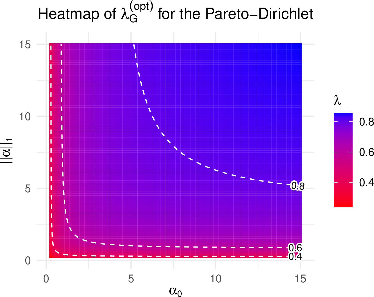
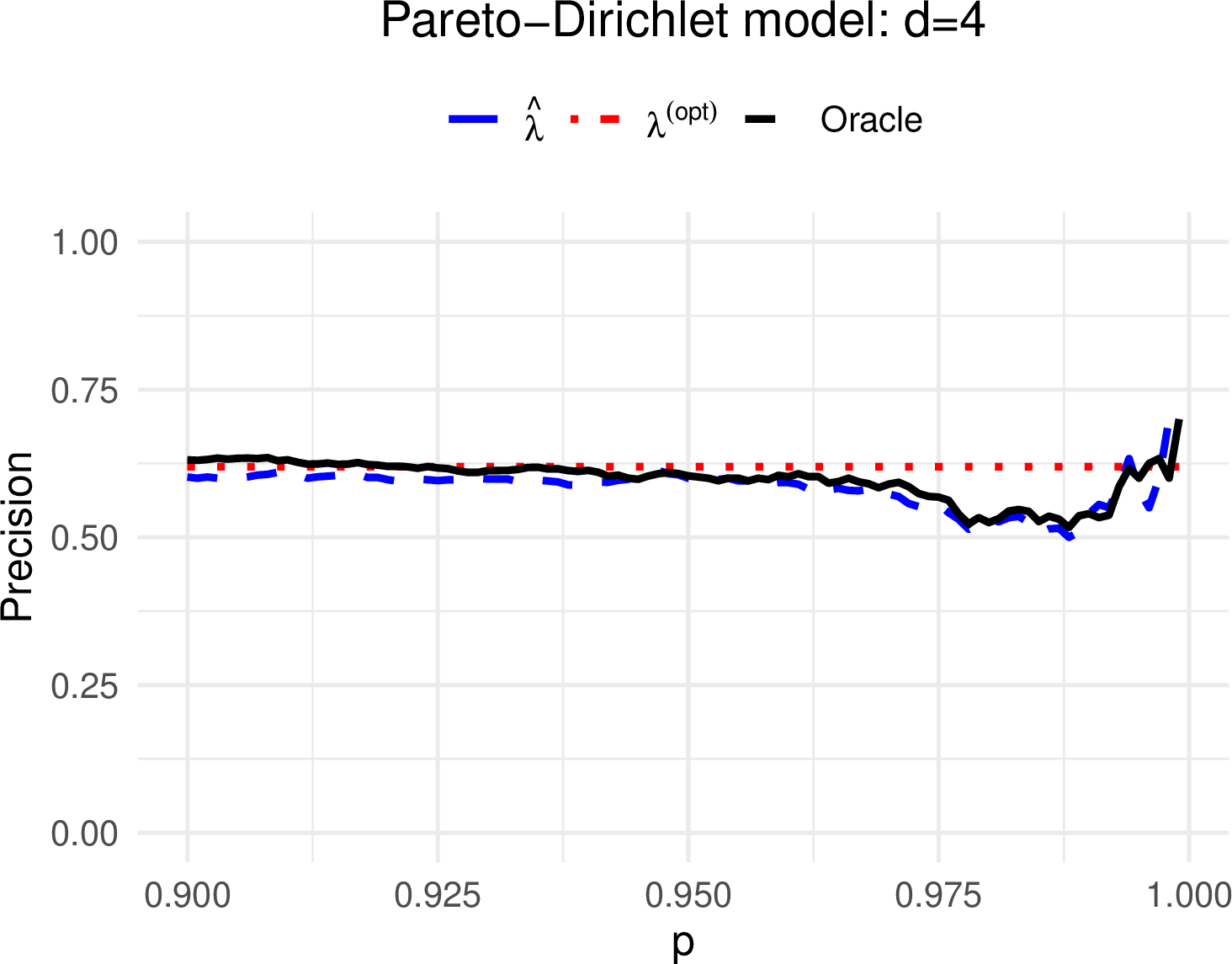
Figure 3: Left panel: Optimal extremal precision \(\lambda_{\cal G}^{\rm (opt)}\) for predicting one component of the Pareto-Dirichlet model via a homogeneous function of the rest 140 . Right panel: The empirical tail-dependence coefficients \(\hat{\lambda}_p\) for: (i) the asymptotically optimal Oracle predictor \(h^{(\rm opt )} (X) \propto \|X\|\) (black solid line) (ii) a non-parametric estimator of the optimal predictor \(\widehat Y := \widehat h(X)\) based on a training and testing samples of size \(n_{\rm train} = n_{\rm test} = 10^4\) (see Section 10)..
9.3 On the sub-optimality of homogeneous predictors↩︎
In some cases, the optimal predictors are in fact homogeneous functions of the covariates (cf Example 4). We will demonstrate next, however, that the class of homogeneous functions does not always contain neither optimal nor asymptotically optimal predictors. The spirit of this example is to show that the extremes of \(X\) do not necessarily predict well the extremes of \(Y\).
Example 8. Let \(\epsilon\) and \(Z\) be independent standard \(1\)-Pareto random variables and \[Y := c Z + (1-c) \epsilon,\] for some \(c\in (0,1]\). Consider the covariate vector: \[X = (X_1,X_2)^\top := (e^{-YZ} + Z, Z)^\top\] taking values in \(\mathbb{R}_+^2\).
Clearly, with \(h^{\rm (opt)} (x) := -\log(x_1-x_2)/x_2,\) \(x = (x_1,x_2) \in \mathbb{R}_+^2\), we have \(Y = h^{\rm (opt)}(X)\), almost surely. Thus, the optimal extremal and non-extremal precisions are equal to \(1\). On the other hand, the intuition that the extremes of \(X\) (defined in terms of some homogeneous radial function \(h\)) will predict the extremes of \(Y\) fails!
Indeed, for every continuous, \(1\)-homogeneous \(h:\mathbb{R}_+^2\to \mathbb{R}_+\) such that \(h(x)>0\), for all \(x\not=0\), it can be shown that \[\lambda(Y, h(X)) = \lambda(Y,Z) = c,\] which can be made arbitrarily small.
10 Practical Implementation↩︎
Many of the existing implementations of quantile regression can accommodate importance weights and thus achieve estimators for the quantiles of the tilted distribution in 21 . Here, we opted for using the versatile
quantile regression forest of [16] and its efficient implementation in the package ranger of [41]. Specifically, this can be achieved with the R commands: \[\begin{align} &\tt weights
<- 1 - u\\ &{\tt data<-data.frame(u=u, theta)}\\ &\tt rf<-ranger(u\sim.,data=data, case.weights=weights, quantreg=TRUE)
\end{align}\] Here \({\tt u}\) and \({\tt \theta}\) are \((n_r\times 1)\) and \((n_r\times d)\) arrays, whose \(i\)th rows correspond to \(U_i\) and the vector \(\Theta_i\), respectively, \(i=1,\cdots,n_r\). The ranger function
returns a random forest S3 object, which can be used to generate predictions of \(\widehat q_\alpha(\theta_{\rm new})\) using the commands \[\begin{align} &{\tt
theta\_new = x\_new/L1\_norm(x\_new)}\\ &{\tt pred <- predict(rf, data=theta\_new, type="quantiles", quantiles=alpha)}\\ &{\tt q\_alpha <- pred\$predictions}
\end{align}\]
The following Algorithm 4 summarizes the inference. The R code implementing the estimator using the ranger package of [41] is given in [18]. An R Shiny App demonstrating the estimator is
deployed on [19], where further covariate selection heuristics are implemented.

Note that the sequence \((\alpha_n)_{n\in \mathbb{N}}\) provided by Algorithm 4 fulfill the assumption of theorem 3 by application of lemma 14.
Lemma 14. If for any \(\theta \in S^d\) the quantile estimator \(\hat{q}_{\alpha_n,n}\) is uniformly consistent on compacts of \((0,1)\), then the sequence \((\alpha_n)_{n\in \mathbb{N}}\subset (0,1)\) defined by the algorithm 4 satisfies \[\alpha_n \underset{n\rightarrow\infty}{\overset{\mathbb{P}}{\longrightarrow}}\alpha_{opt}.\]
Proof of Lemma 14. For \(n \geq 2\) we can write, \[\begin{align} \left\{|\alpha_{opt}-\alpha_n|\leq \frac{1}{2^{n-1}}\right\}=&\left\{|\alpha_{opt}-\alpha_{n-1}|\leq \frac{1}{2^{n-2}}\right\}\bigcap \left\{\exists \;l_0>0 | \forall l>l_0,\frac{q(\alpha_{opt})-\hat{q}_l(\alpha_n)}{q(\alpha_{opt})-q(\alpha_n)}>0\right\}\\ =&\left\{|\alpha_{opt}-\alpha_{2}|\leq 1\right\}\bigcap\left(\bigcap_{k=2}^n \left\{\exists \;l_0>0 | \forall l>l_0,\frac{q(\alpha_{opt})-\hat{q}_l(\alpha_k)}{q(\alpha_{opt})-q(\alpha_k)}>0\right\}\right)\\ =&\bigcap_{k=2}^n \left\{\exists \;l_0>0 | \forall l>l_0,\frac{q(\alpha_{opt})-\hat{q}_l(\alpha_k)}{q(\alpha_{opt})-q(\alpha_k)}>0\right\}.\\. \end{align}\] In the previous equalities, since the number of intersections is finite, we can always use the always integer \(l_0\) in each sets. Hence, taking the complementary in the previous equality, we get \[\mathbb{P}\left(|\alpha_{opt}-\alpha_n|\geq \frac{1}{2^{n-1}}\right)\leq\sum_{k=2}^n\mathbb{P}\left(\exists \;l_0>0 | \forall l>l_0,\frac{q(\alpha_{opt})-\hat{q}_l(\alpha_k)}{q(\alpha_{opt})-q(\alpha_k)}<0\right).\] Noticing that, for all \(k\), \[\left\{\exists \;l_0>0 | \forall l>l_0,\frac{q(\alpha_{opt})-\hat{q}_l(\alpha_k)}{q(\alpha_{opt})-q(\alpha_k)}<0\right\}\subset \left\{\exists \;l_0>0 | \forall l>l_0,|\hat{q}_l(\alpha_k)-q(\alpha_k)| >|q(\alpha_k)-q(\alpha_{opt})|\right\},\] since \(\hat{q}_l\) converge uniformly in probability on \((0,1)\), there exists \(l_n\in \mathbb{N}\) such that, for all \(l >l_n\) \[\mathbb{P}\left(|\hat{q}_l(\alpha_k)-q(\alpha_k)| >|q(\alpha_k)-q(\alpha_{opt})|\right)\leq \frac{1}{n(n-2)},\quad \forall \;2\leq k \leq n.\] This leads to \[\mathbb{P}\left(|\alpha_{opt}-\alpha_n|\geq \frac{1}{2^{n-1}}\right)\leq \frac{1}{n}.\] ◻
11 An application to Solar flare prediction↩︎
In this section, we apply the general optimal homogeneous prediction methodology described in the previous section to an important open problem from space physics [4], [20].
In the following, the responses \(\{Y(t),\;t=1,2,\cdots\}\) come from a curated X-ray flux time series derived from a collection up to 15 different GOES satellite measurements (Figure 5). The
covariates \(X_1(t),\cdots,X_d(t),\;t=1,2,\ldots\) are time series of \(d=22\) statistics referred to as SHARP time series. They are derived from solar disk images and capture
fundamental physical characteristics of the active regions (sun spots) which are believed to drive the formation of solar flares [56], [57].
The objective is to predict extreme flux events \(\{Y(t+h)>y_0\}\) at some future time period \(t+h\), based on \(\{X_i(t),\;i=1,\cdots,d\}\).
The events when the X-ray flux exceeds high thresholds are known as Solar flares and they are classified in several severity classes [58]. We
will focus on predicting the most extreme M- and X-class flares, which correspond to X-ray fluxes exceeding \(10^{-5}\;W/m^2\) and \(10^{-4}\;W/m^2\), respectively (Figure 5).
![Figure 5: Time series of maximum daily X-ray flux (in Watts per square meter). The data is based on the highest quality measurements obtained from merging observations from the GOES satellites [58]. It spans two solar cycles (SC24 & SC25). The horizontal line marks the X-class flare threshold (10^{-4}\;W/m^2).](/article/2606.26270/figs/Xray_flux_time_series.png "fig:")
Standardization. For both the response and the predictors, we consider non-overlapping block maxima over a window \(w\) corresponding to \(24\) hours: \[Y^{(w)} (t):= \max_{ w(t-1)+1 < s\le wt} Y(s)\;\; and \;\;X_{j}^{(w)}(t):= \max_{w(t-1)+1 < s\le wt} X_j(s).\] We then construct estimates \(\widehat F_{Y^{(w)}}\) and \(\widehat F_{X_j^{(w)}}\) of \(Y^{(w)}(t)\) and \(X_j^{(w)}(t)\) based on a training sample \(t\in {\cal D}_{\rm train}\). Tail extrapolation is used to ensure that the CDFs have unbounded supports and define the training sample with standardized approximately \(1\)-Pareto marginals: \[\widetilde{Y}(t) := \frac{1}{1-\widehat F_{Y^{(w)}}(Y^{(w)}(t))} \;\; and \;\; \widetilde{X}_j(t) := \frac{1}{1-\widehat F_{X_j^{(w)}}(X_j^{(w)}(t))},\] for all \(t\in {\cal D}_{\rm train}\), and \(j=1,\cdots,d\).
Then, under the assumption that the so-standardized vectors \((\widetilde{Y}(t+h), \widetilde{X}_1(t),\cdots, \widetilde{X}_d(t)), t, t+h\in {\cal D}_{\rm train}\) are realizations from a jointly regularly varying vector
\((Y,X)\), we apply the inference methodology of Section 4. Specifically, we select the threshold \(r\) as a high quantile of the sample of norms, and
apply the quantile random forest to estimate the optimal homogeneous predictor \(\widehat h\).
Prediction. Given a test sample \({\cal D}_{\rm test}\), we compute \[\widehat Y(t+h) := \widehat h( \widetilde{X}(t)),\;t, t+h\in {\cal D}_{\rm test},\] where \(\widetilde{X}(t) = (\widetilde{X}_j(t),\;j=1,\cdots,d)\) are standardized as: \[\widetilde{X}(t): =\frac{1}{\widehat F_{X_j^{(w)}} (X_j^{(w)}(t))},\;t\in {\cal D}_{\rm test}.\] Recall that
\(\widehat F_{X_j^{(w)}}\) is an estimate of the CDF of \(X_j^{(w)}\) obtained from the training sample.
We predict a certain type of flare whenever \(\widehat Y(t+h)\) exceeds a threshold. Specifically, we let \(\hat{p} := \widehat F_{Y^{(w)}}(u)\) and produce the binary predictors: \[I_t(h):= I\{\widehat Y(t+h) > 1/(1-\widehat p) \}.\] This choice, under the assumption of stationarity, ensures the approximate calibration \(\mathbb{E}[ I_t(h)] \approx \mathbb{P}[
Y^{(w)}(t+h)> u]\). More precisely, for the M- and X-class flares, we use the thresholds \(u=10^{-5}W/m^2\) and \(u = 10^{-4} W/m^2\), respectively. The X-class flares are among
the most extreme and rare events, which can lead to major magnetic storms. While less severe, the M-class flares can also cause major disruption of Earth’s ionosphere and lead to satellite and electric outages.
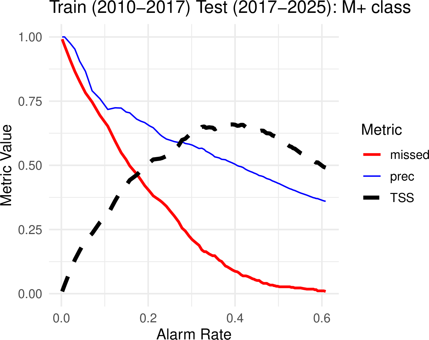
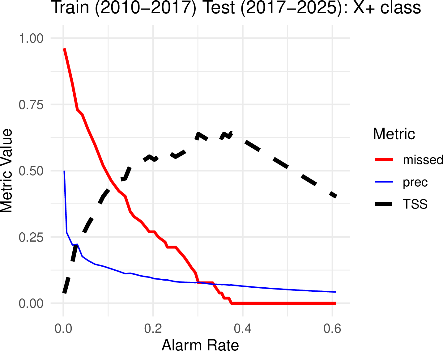
Figure 6: Evaluation metrics for the prediction of M-class (left panel) and X-class (right panel) solar flare events. The homogeneous predictor was based on 24-hour block-maxima of the SHARP time series covariates TOTUSJH,
AREA_ACR, ABSNJZH, SAVNCPP, TOTPOT, and a 24-hour lagged flux. The response is the 24-hour block-maximum flux time series. We used the period of 2010–2017 with \(n_{\rm train}
=1,941\) observations for training and tested on the period 2017-2025 with \(n_{\rm test} = 2,018\) observations. The radius threshold was chosen as the \(0.97\)-th quantile of the
empirical distribution and the quantile random forest was built using \(2000\) trees, i.e., the ranger function was called with parameter num.trees=2000..
Results. Figure 6 shows a simple, nearly tuning-free application of the optimal homogeneous prediction methodology to Solar flare prediction. Specifically, the homogeneous predictor was trained over the period (2010-2017) and applied to forecasting M- and X-class flares over the period (2017-2025). Confusion matrices for the binary forecasts were used to obtain various metrics displayed on the plots. Specifically, letting TP, FP, TN, FN denote true-positive, false-negative, true-negative, and false-negative counts of the predictions, we obtain the standard metrics: \[{\rm prec} = \frac{TP}{TP+FN}, \;\;\text{TSS} = \frac{\mathrm{TP}}{\mathrm{TP} + \mathrm{FN}} - \frac{\mathrm{FP}}{\mathrm{FP} + \mathrm{TN}}, \; and \; {\rm missed} = \frac{FN}{TP+FN}.\] These metrics depend on the chosen quantile \(\tau_p\) for the variable \(\widehat Y=h(\widetilde{X})\), which ultimately determines the alarm rate: \[{\rm alarm} = \frac{{\rm TP} + {\rm FP }}{{ n_{\rm test}}},\] where \(n_{\rm test}\) is the size of the test sample.
As the alarm rate decays, generally, the precision increases but so does the proportion of missed events. Observe that the popular TSS statistic can be non-informative or at best misleading. Indeed, very high values of TSS may be associated with quite poor precision and hence quite high false-alarm rate. On the other hand, well-calibrated predictors with alarm rate equal to the event rate may have quite low TSS values. Nevertheless, the peak of the TSS values seem to be aligned with an elbow in the missed rate, so it happens to be a good heuristic in this case.
In principle, however, in addition to TSS, we advocate for examining the precision and missed metrics, as a function of the alarm rate. The practitioner may choose to settle for an acceptable alarm rate that achieves good precision and low missed rate that may or may not correspond to high TSS. Optimizing a flare prediction method for achieving high TSS without considering calibration or alarm rates could be misleading. This said, the TSS values achieved by the generic optimal homogeneous predictor methodology are surprisingly high. While the best M-class flare forecasting machines claim to achieve TSS rates as high as \(0.7\) (or sometimes \(0.8\) in carefully designed studies), our method reaches \(0.66\) with hardly any tuning at all, should one look at a suitable alarm rate of about \(30\%\). At the same time the existing X-class flare forecasting methods barely reach TSS as high as \(0.5\) in operational settings (i.e., without off-line post-processing of the data, which can often induce hard-to-control leakage of information from the testing data into the training data). The maximum TSS values for our method of predicting X-class flares is \(0.64\), comfortably surpassing the coveted state-of-the-art threshold, should one contend with alarm rate of \(40\%\). While we do not claim to have achieved close to optimal forecasts, this brief analysis demonstrates the great potential of the optimal homogeneous prediction methodology in the solar flare forecasting challenge.