Latent thermal instability
June 24, 2026
Abstract
Multiscale temperature fluctuations are abundant in the intracluster medium (ICM) outside of galaxy cluster cores (\(\sim 100~{\rm kpc}\)). Their origin is often attributed to turbulent stirring by subhalos or accreting baryons crossing the virial radius. However, their apparent resistance to mixing and thermal conduction in a collisional medium has not been explained. We propose a new mechanism by which steady-state temperature fluctuations can form and persist outside the cluster core. Local thermal instability, or Field instability, is used to explain filamentary condensates in cluster cores but is usually dismissed outside them because thermal conduction should suppress instability. In weakly collisional or collisionless plasmas, however, thermal conduction can be anomalously suppressed by heat-flux-driven plasma instabilities triggered in presence of a local magnetic field, leading to two effects: (i) condensates form in a new parameter regime that overlaps with conditions outside the core, and (ii) condensates reach a steady state as in the hydrodynamic limit. This extends the regime of instability-driven fluctuations to over \(\gtrsim50\%\) (depending on hot plasma temperature) of the cluster. We use one-dimensional hydrodynamic simulations of condensates to test our analytical ideas.
1 Introduction↩︎
The regions outside the cores of galaxy clusters have become a new frontier for probing the intracluster medium (ICM), the intergalactic medium, and cosmology, enabled by multi-wavelength synergy between X-ray, Sunyaev-Zeldovich (SZ), and Weak Lensing (WL) observations (see [1] for a review). Cluster thermodynamics is jointly constrained by X-ray and SZ observations, while WL can reveal hydrostatic mass bias. A prime example is the Coma cluster, for which joint observations have revealed pressure fluctuations (e.g., [2], [3]) and density fluctuations at large distances from the core (e.g., [4], [5]). Generally, temperature contrasts outside the cores, on both small and large scales, have been discussed for several decades (e.g., [6]–[10]).
The origins of fluctuations in the ICM outskirts remain debatable, but multiscale temperature, density, and pressure fluctuations perhaps arise from turbulent stirring by accreting plasma or galaxies crossing the virial radius. The puzzling observation is that they do not get erased. For a temperature fluctuation on scale \(\ell\), decay should occur at a rate \(\kappa_{\rm c} T_0/p_0\ell^2\) in a strongly collisional plasma, where \(\kappa_{\rm c}\) is the collisional thermal conductivity ([11]), \(T_0\) the mean temperature, and \(p_0\) the mean pressure of the medium. This timescale is short outside cluster cores compared to merger-duration timescales, yet fluctuations persist ([12]). Temperature structures created on a scale \(\ell\) should also de-cohere on a timescale \(\ell/u_{\ell}\) (where \(u_{\ell}\) is the velocity of the turbulent eddy of size \(\ell\)) in turbulent media; in other words, once these structures have formed, they will be mixed quickly unless persistently stirred. This raises various questions: why do they survive, and is there an alternative mechanism for producing steady-state multiscale temperature fluctuations? In this work, we propose a new solution to this problem.
Thermal instability (TI), driven by radiative cooling in a dilute magnetized plasma, has been widely discussed as an explanation for density fluctuations or condensates, from solar prominences (e.g., [13]) to the intracluster and intergalactic medium on large scales (e.g., [14], subsequently followed up in simulations of globally thermally stable clusters by [15]–[17] and for a mini-review see [18]). In unmagnetized plasma, thermal conduction sets the smallest scale for thermally unstable modes, the Field length \(\lambda_{\rm F}\), below which heat flux dominates over radiative cooling. The linear TI growth rate is scale free. But at large scales, TI transitions from isobaric (\(\delta p/p_0 \ll \delta \rho/\rho_0\)) to isochoric (\(\delta p/p_0 \gg \delta \rho/\rho_0\)) because the sound-crossing time exceeds the radiative cooling time, a point emphasized in recent work on condensation in circumgalactic plasma in smaller dark matter halos (e.g., [19], [20]).
The known effect of magnetic field on TI is twofold: it can affect dynamics directly, enhancing condensation (e.g., [21]–[26]), and it also modifies the nature of thermal conduction (e.g., [27]). In this work, we focus on the effect on conduction. For a collisional plasma, [28] showed that heat transport is anisotropic when \(r_e \ll \lambda_{\rm mfp}\ll \ell_{\rm T,\parallel}\), where \(r_e\) is the electron gyroradius, \(\lambda_{\rm mfp}\) is the Coulomb collisional mean free path, and \(\ell_{\rm T,\parallel}\) is the temperature-gradient scale along the field (which may in principle differ from the size of temperature fluctuations). This is because electrons are constrained to gyrate about the local magnetic field. A tangled magnetic field therefore channels heat along field lines and suppresses the effective isotropic heat flux by a factor of \(\sim 3-5\) ([29]), a point discussed in the context of cooling flows in galaxy clusters ([30]–[32]). For TI, this implies that a local patch of tangled field may support fine-structured condensates, but overall the turbulent ICM behaves like a hydrodynamic medium. The key problem therefore remains: classical anisotropic conduction is expected to erase TI-driven temperature contrasts on relatively short timescales, especially far from cluster centers, since the radiative cooling time increases with radius (see [33] for constraints on filament sizes across background temperatures).
However, this conclusion overlooks the anomalous transport properties of weakly collisional and collisionless plasmas. Since density decreases with radius in galaxy clusters, the collisional mean free path becomes larger than in the core, so \(\lambda_{\rm mfp}\lesssim \ell_{\rm T}\). In a collisionless medium, non-local effects can regulate heat transport because fast electrons stream along magnetic fields ([34]). In addition, if magnetization is weak, microscale electromagnetic plasma instabilities also anomalously regulate transport ([35]). The condition for the heat-flux-driven whistler instability, a kinetic electromagnetic microinstability that grows at electron Larmor scales ([36], [37]), is \(\beta_e \lambda_{\rm mfp}/\ell_{\rm T}\gtrsim 1\), where \(\beta_e=8\pi p_0/B^2_0\) is the ratio of thermal pressure (\(p_0\)) to magnetic pressure (\(B^2_0/8 \pi\)), and this condition is often satisfied in the ICM. Particle-in-cell simulations across a range of \(\ell_{\rm T}\) and numerical setups robustly show that this instability suppresses the free-streaming heat flux by a factor proportional to \(\beta_e\) ([38]–[42]). The whistler waves scatter electrons in pitch angle, limiting transport to the whistler phase speed. Recent laser-plasma experiments have also hinted at suppressed thermal conduction in high-\(\beta_e\) plasmas ([43], [44]). In galaxy clusters, \(\beta_e \lambda_{\rm mfp}/\ell_{\rm T}\) spans a wide range, so classical transport models may not provide the most accurate description of thermal conduction everywhere.
Some effort has already been made to assess the role of anomalous transport in modifying fluid instabilities (see [45], [46]); here, we examine for the first time the effect of anomalous conduction on TI. We identify a condensation regime below the classical Field length, which we call Latent TI (LaTI). We develop one-dimensional (1D) hydrodynamic simulations, assuming cylindrical hot plasma filaments aligned with a coherent magnetic field, parameterized by the electron plasma \(\beta_e\) and the perturbation size corresponding to the initial coherence scale \(\propto k_0^{-1}\), with \(k_0\) the wave number, to validate the LaTI regime and explore basic condensate properties when the filament grows clumps along itself.
In section 2, we describe the theoretical preliminaries and physical assumptions. In section 3, we discuss the 1D hydrodynamic simulations and LaTI properties. In section 4, we apply LaTI to the galaxy-cluster context, and in section 5, we conclude.
2 Theoretical preliminaries↩︎

We consider a 1D medium in the \(\hat{\boldsymbol{x}}\) direction, aligned with the local magnetic field and thus cylindrically symmetric, with approximately uniform number density (\(n=n_e\sim
n_i\)) and temperature (\(T=T_i\sim T_e\)), where the subscripts \(e,i\) denote electrons and ions, respectively. Electron-ion collisions cause electrons to accelerate and emit
radiation at a rate proportional to \(T_e^{{1}/{2}}\) via Bremsstrahlung cooling, such that the rates of ionization and recombination are balanced. We assume that the medium is heated on average at the rate \(\mathcal{H}=\langle \zeta \rangle\), where \(\zeta\) is the radiative cooling rate. This heat is supplied by energy sources such as AGNs, supernovae, or mergers, the details of which are ignored
for the present purpose1. The medium is collisional and follows mass, momentum, and energy conservation according to hydrodynamic evolution (\(\lambda_{\rm mfp}\ll \ell_{{\rm T}}\)). The equations relevant to such an evolution are the following: \[\begin{align} \tag{1}
\frac{D \rho}{Dt} &=& -\rho \boldsymbol{\nabla}\cdot \boldsymbol{v},\\
\tag{2}
\frac{D \boldsymbol{v}}{Dt} &=& -\frac{\boldsymbol{\nabla}p}{\rho}, \\
\tag{3}
\frac{p}{\gamma - 1} \frac{D \ln \left({p}/{\rho^{\gamma}}\right)}{Dt} &=& -\mathcal{\zeta} +\mathcal{H} + \boldsymbol{\nabla} \cdot \left({\kappa_{\rm (c,a),\parallel} \boldsymbol{\nabla} T}\right),
\end{align}\]
where \(\frac{D}{Dt}= \frac{\partial}{\partial t} + \boldsymbol{v}\cdot \boldsymbol{\nabla}\) is the Lagrangian derivative, \(p\), \(\rho\), \(T\), and \(\boldsymbol{v}\) are the pressure, density, temperature, and velocity (which is approximately the bulk velocity \(\boldsymbol{v}_i\) of the ions) of
the fluid, and \(\gamma=5/3\) is the adiabatic index of an ideal gas. In eq. 3 , the last term is related to the parallel heat flux \(\mathcal{Q}\), given by \[\mathcal{Q} = \kappa_{\rm (c,a), \parallel} \boldsymbol{\nabla_{\|}} T.\]
For a collisional plasma, parallel heat transport is governed by collisions of free electrons with background electrons and ions parallel to the local magnetic field, and so the parallel thermal conductivity in this case is, \[\label{eq:32clascond} \kappa_{\rm c,\parallel} = 2.6\times 10^{11} \left({\frac{T}{\rm keV}}\right)^{\frac{5}{2}}~{\rm erg~{cm}^2~s^{-1}{K}^{-1}}.\tag{4}\] If a local patch of this medium evolves such that \(\lambda_e \beta_e\gg \ell_{{\rm T},\parallel}\), kinetic instabilities are expected to suppress the heat flux (free-streaming electrons) down a temperature gradient by a factor \(\beta_e^{-1}\). Since the medium around galaxies has a large \(\beta_e\), this modification to transport may occur in such media, particularly at large radii away from the central galaxy. A proposed sub-grid closure for parallel thermal conductivity in such a scenario is ([39]), \[\label{eq:32anocond} \kappa_{\rm a, \parallel} = \frac{2.6\times 10^{11}}{1+ \mathcal{A}\lambda_e \beta_e/\ell_{{\rm T},\parallel} } \left({\frac{T}{\rm keV}}\right)^{\frac{5}{2}}~{\rm erg~{cm}^2~s^{-1}{K}^{-1}},\tag{5}\] where we used \(\mathcal{A}=0.53\) and \(\ell_{{\rm T},\parallel}={|\boldsymbol{\nabla}_{\parallel}\ln T|}^{-1}\), the scale of the temperature gradient along the local magnetic field. Thermal conductivity thus smoothly interpolates between the classical and anomalous regimes. In our current work, we consider a plasma at fixed plasma \(\beta_e\). We also use the following for the collisional mean free path: \[\label{eq:mfp} \lambda_e = 0.003 {\left( \frac{T}{{\rm keV}} \right)}^2{\left(\frac{n}{0.1~{\rm cm}^{-3}}\right)}^{-1}~{\rm kpc}.\tag{6}\] The RHS of eq. 3 in exact balance (\(\mathcal{H}=0\)) defines the Field length for classical conduction, which we express as follows: \[\label{eq:fldlen} \lambda_{\rm F}=9.63 {\left( \frac{T}{{\rm keV}} \right)}^{5/4}{\left( \frac{\tau_{\rm cool}}{1~{\rm Gyr}}\right)}^{1/2}{\left(\frac{n}{0.1~{\rm cm}^{-3}}\right)}^{-1/2}~{\rm kpc} ,\tag{7}\] where the cooling time is \[\label{eq:coolt} \tau_{\rm cool} = 0.09 {\left(\frac{T}{{\rm keV}}\right)}^{1/2}{\left(\frac{n}{0.1~{\rm cm}^{-3}}\right)}^{-1}~{\rm Gyr}.\tag{8}\] Below this scale, conduction is expected to erase temperature fluctuations. The decay timescale for a given length scale \(\ell\) due to classical conduction is \[\label{eq:condt} \tau_{\rm c} = 0.03 {\left(\frac{\ell}{1~{\rm kpc}}\right)}^2{\left( \frac{T}{{\rm keV}}\right)}^{-5/2} \left(\frac{n}{0.1~{\rm cm^{-3}}}\right) ~{\rm Gyr}.\tag{9}\] We also frequently consider the characteristic length scale that sound crosses in a cooling time, \[\label{eq:lams} \lambda_{\rm s} = c_{\rm s}\tau_{\rm cool}=45 \left( \frac{T}{{\rm keV}} \right)\left(\frac{n}{0.1~{\rm cm^{-3}}}\right)^{-1}~{\rm kpc} ,\tag{10}\] and the associated sound-crossing timescale over a length \(\ell\): \[\begin{align} \label{eq:32sndt} &\tau_{\rm snd}& = 0.002\left(\frac{\ell}{1~{\rm kpc}}\right) {\left( \frac{T}{{\rm keV}}\right)}^{-1/2}~{\rm Gyr}. \end{align}\tag{11}\]
2.1 What happens to the TI criterion?↩︎
In terms of microphysical quantities, the classical parallel conductivity scales as \(\kappa_{\rm c,\parallel}\sim n_e \lambda_e v_{{\rm th},e}\). It follows that TI growth is suppressed by conduction under the following
condition on the rates of the two processes at a wavenumber \(k_{\ell}\) associated with the length scale \(\ell\): \[\label{eq:clasField}
{k^2_{\ell} \lambda_{e0} v_{{\rm th}e0}}\ll \tau^{-1}_{\rm cool0},\tag{12}\] where the subscript \(0\) denotes mean quantities of the hot medium, rather than fluctuations. For short wavelengths of thermally
unstable fluctuations (isobaric), the exact growth rate is \[\label{eq:32isob}
\sigma_{\rm ib} =\frac{(2 - \Lambda_{\rm T}) }{\gamma \tau_{\rm cool0}},\tag{13}\] and for long wavelengths (isochoric) the growth rate is \[\label{eq:32isoc}
\sigma_{\rm ic} = - \frac{\Lambda_{\rm T}}{\tau_{\rm cool0}},\tag{14}\] where the radiative cooling rate is \(\zeta_0 = \rho^2_0\Lambda(T_0)/{(\mu m_p)}^2\), \(\mu\) is the
mean molecular mass, \(m_p\) is the proton mass, and \(\Lambda_{\rm T}= \partial \ln \Lambda/\partial \ln T\). Alternatively, we use the timescales \(\tau_{\rm
ib}\) and \(\tau_{\rm ic}\) for isobaric and isochoric growth/decay timescales. The RHS of eq. 12 should be the actual growth rate of a given unstable mode, but we ignore that detail in
the approximate equations above. The Field length is \[\label{eq:field}
\lambda_{\rm F} \sim \sqrt{\lambda_{e0}v_{{\rm th}e0} \tau_{\rm cool0}}.\tag{15}\] If \(k_{\ell} \beta_e \lambda_e \gg 1\), eq. 5 gives the thermal conductivity and the condition
on the rates for TI to happen is the following: \[\begin{align}
\label{eq:32anoField}
\frac{k_{\ell}v_{{\rm th}e0}}{\beta_{e0}} \ll \tau^{-1}_{\rm cool0},
\end{align}\tag{16}\] or, equivalently, \[\begin{align}
\frac{\tau_{\rm cool0}}{\tau_{\rm snd0}}\ll \beta_{e0} \sqrt{\frac{m_e}{m_i}}.
\end{align}\]
Therefore, the anomalous TI condition sets a new length scale below which anomalous thermal conduction interferes with TI growth. \[\label{eq:32ano95lmin}
\lambda_{\rm a} \sim \frac{\lambda_{\rm s}}{\beta_{e0}}\sqrt{\frac{m_i}{m_e}}.\tag{17}\] We can write the ratio of the minimum scales for the onset of TI as \[\label{eq:32l95ratio}
\frac{\lambda_{\rm a}}{\lambda_{\rm F}} \sim \frac{668}{\beta_{e0}} {\left(\frac{T}{{{\rm keV}}}\right)}^{-\frac{1}{2}}.\tag{18}\] For a \(10~{\rm keV}\) plasma with \(\beta_{e0}\sim
1000\), \(\lambda_{\rm a}/\lambda_{\rm F}\sim 0.2\). This implies that anomalous conduction could allow scales orders of magnitude below the classical Field length to remain unstable depending on the plasma \(\beta_e\). Fig. 1 shows the LaTI regime based on the inequality in eq. 16 . The yellow region defines the usual TI parameter space. The diagonal line determines the
changes in the length scale of a perturbation (\(k_0\)). The red region shows the parameter space in which the heat-flux-driven whistler instability is active. Within the red area, the purple region defines LaTI. We verify
this parameter space by carrying out simulations at different \(k_0\) as described in section 3.

2.2 What are the saturation mechanisms?↩︎
If we consider energy conservation for the cooling plasma at early times with linearized perturbations (\(\Lambda_{\rm T}=0.5\)), the terms related to advection, TI, and conduction in the following dominate the energy budget: \[\begin{align} \nonumber \sigma_{\rm adv}\sim\frac{\gamma c_{\rm s0}}{\ell}, \sigma_{\rm TI}\sim\frac{3}{2}\tau_{\rm cool0}^{-1}, \sigma_{\rm (c,a)}\sim\frac{\kappa_{\rm (c,a), \parallel} T_0(\gamma-1)}{\ell^2 p_0}, \end{align}\] where \(\ell\) is the perturbation length scale and \(\kappa_{\parallel (c,a)}\) indicates classical or anomalous conduction. Advection and conduction are the two possible saturation mechanisms competing with the growth term above. We define a dimensionless number, analogous to the thermal Prandtl number, that indicates the likely saturation mechanism for a given initial scale \(\ell\), \[\label{eq:32dimlno} \mathcal{P}{\mathbb{a}} = \frac{\sigma_{\rm adv}}{\sigma_{\rm (c,a)}} = \frac{p_0 c_{\rm s} \ell}{\kappa_{\rm (c,a), \parallel}T_0(\gamma -1)}.\tag{19}\] This dimensionless number is \({\mathcal{P}{\mathbb{a}}}_{\rm c}=\lambda_{\rm s} \ell/\lambda^2_{\rm F}\) and \({\mathcal{P}{\mathbb{a}}}_{\rm a}=\beta_e \sqrt{m_e/m_i}\) for classical and anomalous conduction, respectively. If \(\mathcal{P}{\mathbb{a}}\ll1\), conduction dominates. At steady state, the perturbations reach high density, low temperature, and zero velocity if they are divergence-free. At the peak of the perturbations, \(\partial T/\partial x=0\) and \(\partial^2T/\partial x^2\neq0\), so classical conduction may take over and the final size is then set by approximately the classical Field length at the final temperature and density. By contrast, \(\mathcal{P}{\mathbb{a}}\gg1\) implies that advection drives the dynamics, and the final scale is proportional to the initial temperature-perturbation scale before the onset of TI. Classical conduction may still act on the clump edges in this case, but may not set the final length scale.
3 1D Hydrodynamic simulations↩︎
We use the PLUTO code ([47]) to solve the hydrodynamic eqs 1 3 with
parameter \(\beta_e\), effectively modeling a cylindrical hot plasma along the magnetic field. We use a super-timestepping scheme for thermal conduction and fix the parabolic Courant number by comparing 1D tests of
temperature-fluctuation decay with analytical expectations. We use periodic boundary conditions and a uniform grid size \(N\) with the box size \(L_0\approx 2.4\ell_{\rm T,\parallel0}\). For
the initial condition, we take a simple spatial temperature profile in pressure equilibrium (low density corresponds to high temperature): \[\label{eq:temp95ini}
T(x) = \bar{T}\left(1- A \sin (k_0 x)\right) .\tag{20}\] We use \(\varepsilon=k_0\lambda_{e0}\beta_{e0}\) as a parameter, and all basic simulation parameters are listed in Table
¿tbl:tab:thetab?. All definitions used in the simulations are identical to those in section 2.
| \(\bar{T},\bar{n}\) | \(\varepsilon=k_0\lambda_{e0}\beta_{e0}\) | \(A, \ell_{{\rm T},\parallel0}\) | C/H | \(N\) |
|---|---|---|---|---|
| \(1,2.2\) | \(36.4\) | \(0.2, 25\) | n | \(2048\) |
| \(1,2.2\) | - | \(0.2, 25\) | n | \(2048\) |
| \(1,2.2\) | \(364\) | \(0.2, 25\) | n | \(2048\) |
| \(8,0.1\) | \(256\) | \(0.2, 25\) | n | \(2048\) |
| \(8,0.9\) | - | \(0.9, 5\) | y | \(4096\) |
| \(8,0.9\) | - | \(0.9, 250\) | y | \(16384\) |
| \(8,0.9\) | \(284\) | \(0.9, 2.5\) | y | \(4096\) |
| \(8,0.9\) | \(142\) | \(0.9, 5\) | y | \(2048\) |
| \(8,0.9\) | \(142\) | \(0.9, 5\) | y | \(4096\) |
| \(8,0.9\) | \(28\) | \(0.9, 25\) | y | \(4096\) |
| \(8,0.9\) | \(2.8\) | \(0.9, 250\) | y | \(16384\) |
| \(8,0.9\) | \(2.8\) | \(0.9, 250\) | y | \(8192\) |
3.1 Tests with classical and anomalous decay↩︎
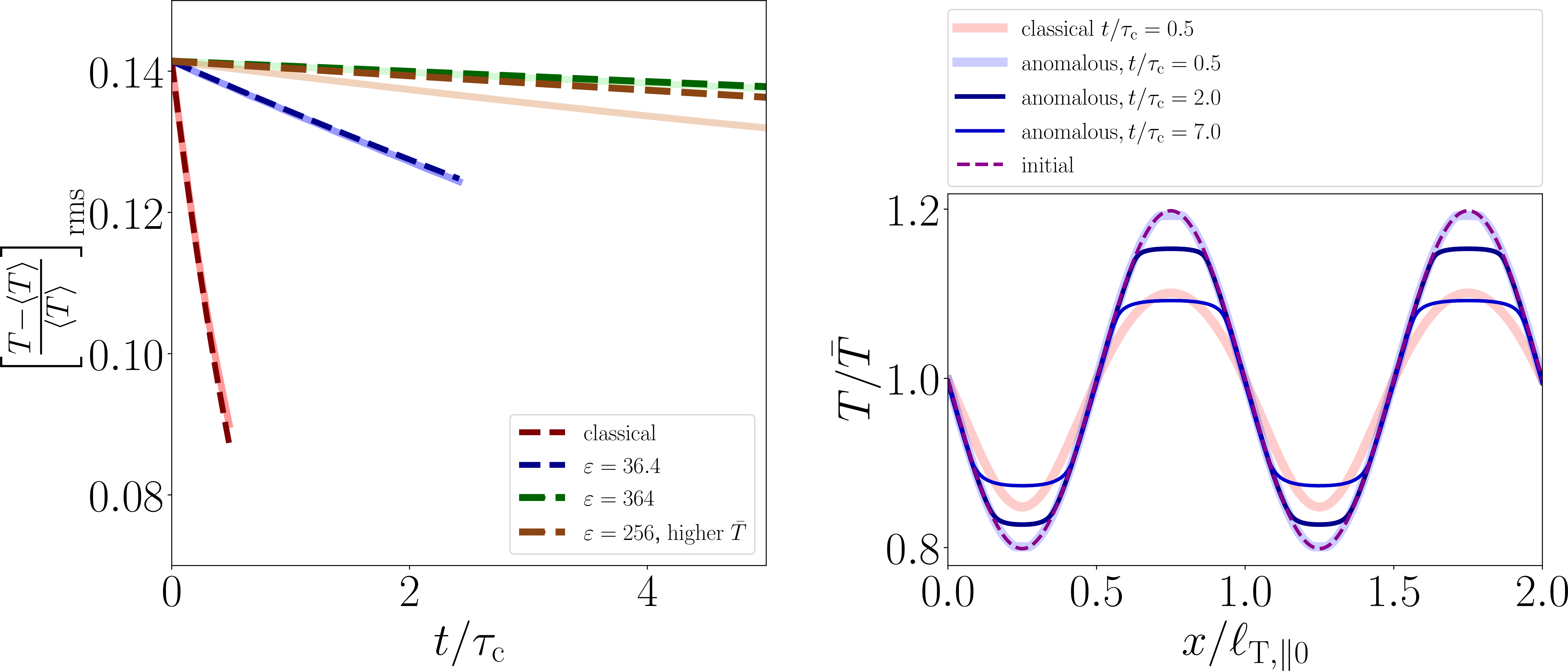
We carry out several tests to compare how classical and anomalous conduction produce distinct temperature-fluctuation evolutions. For a range of \(\varepsilon\), we evaluate the root-mean-squared (rms) temperature fluctuation in the simulation box over time in Fig. 2 (left panel). We normalise time by the classical decay timescale, \(\tau_{\rm c}\). As expected, the decay is slower by a factor proportional to \(\varepsilon\). The right panel compares the classical and anomalous simulations for a given \(\varepsilon\). The fluctuations decay slowly as predicted, but each coherent temperature structure also shows unique features. The fluctuation peak is flattened relative to classical conduction as \(\partial T/\partial x\) approaches zero and classical conduction is activated. However, near the bottom of a temperature peak, \(\partial T/\partial x\) is larger, leading to the maintenance of this approximate step function.
3.2 Tests with radiative cooling↩︎
We carry out several simulations with cooling/heating as described in section 2. Thermal instability causes runaway cooling for dense clumps, and the resulting scale separation in the non-linear stage is especially challenging to capture when thermal conduction is included. Therefore, we impose a temperature ceiling (\(2\times 10^8~{\rm K}\)) and floor (\(2\times 10^6~{\rm K}\)) in our simulations. While this approach artificially flattens temperature peaks and troughs, it also reflects the behavior of a stable-phase plasma in which the TI growth rate is small. In fact, at \(2\times 10^6~{\rm K}\), TI may not exist, depending on the plasma density (as characterized for a given density in Fig. 6 by [20]).
We design four simulations with modified conduction over a range of \(k_0\), as given in Table ¿tbl:tab:thetab? and shown in Fig. 1, spanning the LaTI regime. We also carry out two equivalent simulations with \(\ell_{\rm T,\parallel0}\in [5,250]~{\rm kpc}\) using only classical conduction for comparison. The first two columns in Fig. 3 show the four condensates after saturation in the LaTI regime. For the two smaller perturbation sizes of the four, the initial \({\mathcal{P}{\mathbb{a}}}_{\rm c}\) is less than unity; in other words, advection may not strongly oppose cooling, but conduction will. The final size \(\ell_{\rm f}\) of the condensate is \({\sim}\lambda_{\rm F6}\), the Field length at \(2\times 10^6~{\rm K}\) (upper panel of the last column). Large-scale perturbations scale down such that \(\ell_{\rm f}/\ell_{\rm T,\parallel0}\) is constant in both cases. Classical conduction does not contribute significantly to the final size.
The lower panel of the last column shows the rms density fluctuations over time (normalised to initial \(\tau_{\rm cool0}\)). The dark blue line, which shows LaTI for \(k_0\lambda_{\rm F}=50\), clearly grows to amplitudes as large as the nearly isochoric cases (light blue and red). The onset closely matches the isobaric TI, as expected (also see Fig. 1). For the classical and anomalous cases with \(k_0\lambda_{\rm F}=1\), a distinct feature is that classical conduction causes the amplitude to decay after a few cooling times. This decay rate is approximately equal to the inverse of \(0.2~{\rm Gyr}\) (orange dotted line). To verify this in simulation, we plot in the inset the predicted timescales \(\tau_{\rm c6}, \tau_{\rm ib6}, -\tau_{\rm ic6}\) corresponding to classical decay (orange), isobaric growth, and isochoric growth (decay) at \(2\times 10^6~{\rm K}\) across the mean density in the box at all times. These predicted rates are only relevant beyond \(t\gtrsim \tau_{\rm cool0}\), when the classical decay timescale drops rapidly as the condensate shrinks, until it equals the isobaric timescale. Therefore, even in the traditional TI regime, anomalous conduction insulates saturated large-scale condensates against mixing with the surrounding medium.
4 Implications for cluster outskirts↩︎
4.1 LaTI in an isothermal ICM↩︎
We consider an isothermal model of the galaxy cluster atmosphere to assess at which radii LaTI can operate. We denote all variables at the cluster’s virial radius with the subscript ‘\({\rm vir}\)’. The virial
temperature and virial radius (\(R_{\rm vir}\)) scale with the total mass of the cluster’s dark matter halo (\(M_{\rm vir}\)). \[\begin{align}
\label{eq:Tvir} \left(\frac{T_{\rm vir}}{\rm keV}\right) &=& \frac{2\mu m_p G}{3k_{\rm B}{\rm keV}}{\left[\frac{4}{3}\pi (200\rho_{\rm crit}) \right]}R^2_{\rm vir} \\ \nonumber &=& 2.3{\left(\frac{R_{\rm vir}}{\rm Mpc}\right)}^2,
\end{align}\tag{21}\] where \(G\) is the gravitational constant, and \(\rho_{\rm crit}=10^{-29}~{\rm gm~cm^{-3}}\) is the critical density of the Universe at the current time.
For \(T_{\rm vir}=4~{\rm keV}\), we find \(R_{\rm vir}=1.3~{\rm Mpc}\). The temperature is constant throughout the ICM, and the density falls off as the square of radius. Using flux freezing
for the magnetic field, it follows that \[\label{eq:virial}
\rho_0 (R) = \frac{\rho_{\rm vir} R^2_{\rm vir}}{R^2}, \, T_0(R) = T_{\rm vir}, \, B_0(R) \propto \rho_0^{{2}/{3}}(R).\tag{22}\]
Using the above, the classical and anomalous TI growth conditions (inequalities 12 and 16 ) become, respectively, \[\begin{align}
\tag{23}
\frac{R^2}{R^2_{\rm vir}} &\ll& \frac{1}{k_{\ell}\lambda_{\rm F, vir}},\\
\tag{24}
\frac{R^2}{R^2_{\rm vir}} &\ll& 3.2\times10^{-5}\frac{{\beta_{e,{\rm vir}}}^{{3}/{2}}}{{\left(k_{\ell}\lambda_{\rm F, vir}\right)}^{{3}/{2}}}{\left(\frac{T_{\rm vir}}{\rm keV}\right)}^{{3}/{4}}.
\end{align}\]
The second inequality applies only if conduction is anomalously suppressed, which requires \[\label{eq:anom95vir}
\frac{R^2}{R^2_{\rm vir}} \gg \frac{145}{{\left(k_{\ell}\lambda_{\rm F,vir} \right)}^{{3}/{4}}}{\beta_{e,{\rm vir}}^{-3/4}\left(\frac{T_{\rm vir}}{\rm keV}\right)}^{-{3}/{8}} .\tag{25}\] Additionally, these conditions apply only when a TI
mode fits within a given radius, so \(k_{\ell} R_{\rm max}\sim k_{\ell}\lambda_{\rm F}\) and \(k_{\ell} R_{\rm max}\sim k_{\ell}\lambda_{\rm m}\) set the two feasibility conditions for the
two conductivities. This gives the following scalings for the maximum radius; in the anomalous case, it depends on the virial temperature and plasma \(\beta_{e,{\rm vir}}\): \[\begin{align}
\tag{26}
\frac{R_{\rm max, c}}{R_{\rm vir}} &=& \frac{R_{\rm vir}}{\lambda_{\rm F, vir}}\sim 0.3{\left(\frac{T_{\rm vir}}{\rm keV}\right)}^{-1}, \\
\tag{27}
\frac{R_{\rm max, a}}{R_{\rm vir}} &=& 10^{-9}{{\beta_{e,{\rm vir}}}^{3}}{\left(\frac{R_{\rm vir}}{\lambda_{\rm F, vir}}\right)}^{3}{\left(\frac{T_{\rm vir}}{\rm keV}\right)}^{{3/}{2}}.
\end{align}\]
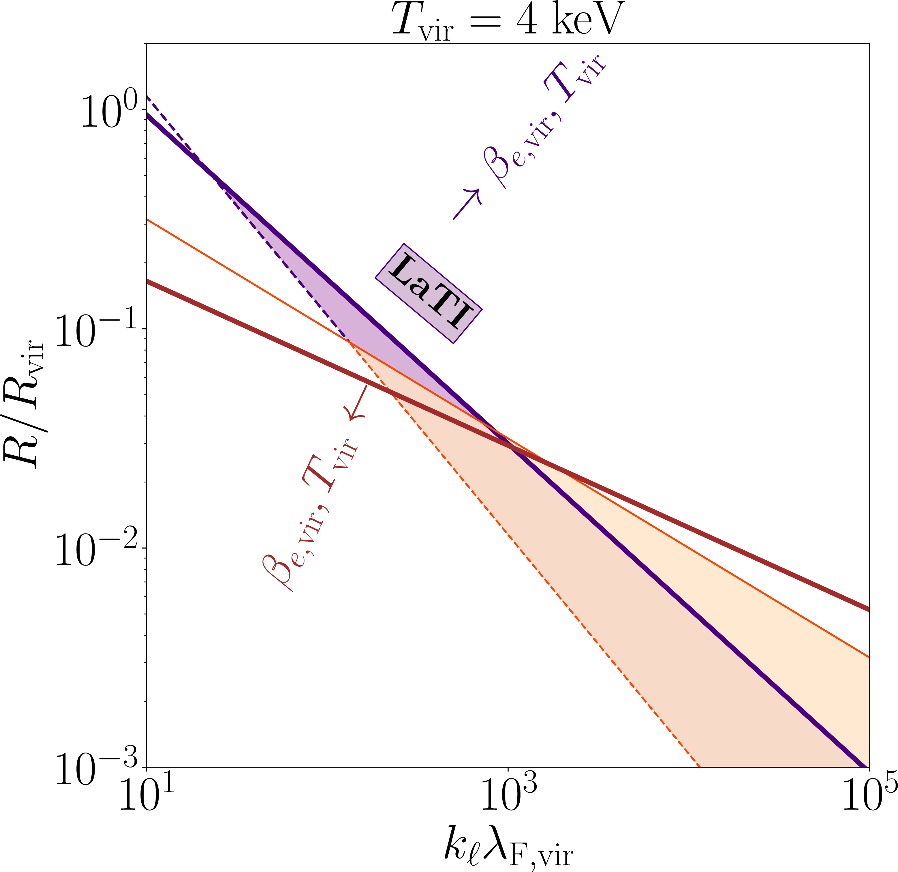
Fig. 4 shows these conditions in parameter space for a galaxy cluster, with fractional radial extent on the \(y\)-axis and size relative to the Field length at the virial radius on the \(x\)-axis. The orange region between the solid thin and the dashed orange lines, respectively, is the classical TI growth regime constrained by mode-size limits at any radius. This lies within a relatively small inner fraction
of the ICM (\(R_{\rm max,c}/R_{\rm vir} \approx 0.07\)). The solid indigo line marks the LaTI condition, and the red line marks the anomalous-effect condition. The purple shaded region is the LaTI regime, extending to \(\gtrsim50\%\) of the cluster (\(R_{\rm max,a}/R_{\rm vir} \approx 0.5\)) and overlapping with the classical regime (excluding about \(5\%\) from the center).
From eqs. 26 27 , we note that the constraint on fitting an unstable mode within a radius depends on the hot plasma’s temperature and may enhance or reduce the LaTI radial extent. In addition,
the LaTI regime is expanded for larger plasma \(\beta_e\) due to suppression of heat flux by a factor \({\sim}\beta^{-1}_e\). This is true for all \(\beta_e
\lesssim \ell_{\rm T,\parallel}/r_e\) ([48]), which is an exceptionally weak constraint for the smallest magnetic field in the ICM (\(\ell_{\rm T,\parallel}/r_e \sim 10^{12}{-}10^{14}\)) to trigger heat-flux suppression.
4.2 How does LaTI compete with turbulent stirring?↩︎
A key question in the context of LaTI in the ICM is whether LaTI can produce abundant small-scale temperature fluctuations instead of turbulent stirring. This addresses the problem of persistent, steady-state temperature fluctuations in the ICM. We consider an outer scale \(\ell_0\) at which energy is injected, and a second scale \(\ell_{\rm C}\) at which the energy-injection rate equals the cooling rate. Using Kolmogorov scaling for turbulent velocities, we equate the eddy turnover timescale to the cooling timescale to determine \(\ell_{\rm C}\): \[\begin{align} \frac{\ell_{\rm C}}{u_{\rm C}} &\sim& \frac{\ell_0}{u_0} {\left( \frac{\ell_{\rm C}}{\ell_0}\right)}^{{2}/{3}} \sim \tau_{\rm cool}, \end{align}\] which gives \[\begin{align} \label{eq:turb} \frac{\ell_{\rm C}}{\ell_0} &\sim& {\left( \frac{\tau_{\rm cool}}{\tau_{{\rm snd},\ell_0}} \mathcal{M}\right)}^{{3}/{2}} \propto R^{3/2}. \end{align}\tag{28}\] We note that the classical Field length \(\propto R^2\) and the constraint on the size of unstable modes \(k^{-1}_{\ell}\propto R\), therefore \(\ell_{\rm C}\) surpass the constraint on size at a smaller cluster radius than where it reaches the Field length. Hence \(\ell_{\rm C}\sim \ell_0\sim R_{\rm turb}\) sets the radius beyond which turbulence is dominant over condensation since the size constraint resists LaTI. For a \(4~{\rm keV}\) plasma as in Fig. 4, we find \(R_{\rm turb}\lesssim R_{\rm max,c}\). Although the onset of LaTI could be affected by turbulence beyond this radius, multi-dimensional numerical simulations show that turbulence and TI can enhance each other non-linearly ([49], [50]).
5 Conclusions↩︎
We propose a new mechanism for producing temperature fluctuations outside the core of the intracluster medium. X-ray surface-brightness and SZ pressure maps suggest that clusters are permeated by persistent density, pressure, and temperature fluctuations. Thermal instability, or Field instability, can operate only within \(\sim 7{-}8\%\) of the cluster core to form low-temperature condensates, since thermal conduction damps fluctuations beyond that extent. However, much of the region outside the core has a collisional mean free path large relative to the temperature-gradient scale, and a weak magnetic field can easily trigger microinstabilities, specifically heat-flux-driven whistlers, that suppress heat flux. This opens a new parametric regime, which we call ‘Latent thermal instability’ (LaTI), in which unstable modes can grow across nearly \(20-70\%\) of the cluster, depending on the hot medium’s temperature, and provide a viable mechanism for steady-state isobaric and isochoric fluctuations throughout this radial range. We use high-resolution 1D hydrodynamic cloud simulations to test our analytical prediction. Testing this proposed mechanism in full MHD models of galaxy clusters remains essential for future work.
PPC acknowledges a computational resource award from the DiRAC High Performance Computing facility. This work used the DiRAC Data Intensive service (CSD3) at the University of Cambridge, managed by the University of Cambridge University Information Services on behalf of the STFC DiRAC HPC Facility (www.dirac.ac.uk). The DiRAC component of CSD3 at Cambridge was funded by BEIS, UKRI and STFC capital funding and STFC operations grants. DiRAC is part of the UKRI Digital Research Infrastructure. PPC and AFAB have also been primarily supported by UKRI (grant number MR/W006723/1) during the course of this research.
PPC conceptualised the problem, performed analytical calculations, simulations, data analysis, and wrote the manuscript. AFAB actively participated in discussions on the results, and final stage of the manuscript.
References↩︎
It is not entirely clear how the hot atmospheres in clusters are maintained in overall thermal equilibrium, but the assumption is justified by the energy budget from the aforementioned heat sources.↩︎