Dissipative Quantum Multiplicative Weights with Sampling Feedback: A Classically Hard Primitive Realized via Engineered Open-System Dynamics
June 24, 2026
Abstract
We introduce Dissipative Quantum Multiplicative Weights with Sampling Feedback (DQMW-Sample), an online-learning primitive in which engineered open quantum-system dynamics prepare a Gibbs state whose computational-basis measurement supplies the loss feedback. The central conceptual contribution is to lift the computational hardness of constant-temperature Gibbs sampling into a physically realizable online-learning primitive. By engineering a Davies-type dissipator whose per-round feedback cannot be efficiently simulated classically, we obtain a learning-theoretic separation in which DQMW-Sample achieves asymptotically sublinear regret while every efficient classical learner suffers constant average regret on a suitably constructed instance. We further prove that the spectral gap of the engineered dissipator contracts hardware noise, yielding sublinear noise-induced regret under a balanced dissipation schedule, and we strengthen the single-round hardness to the full adaptive interaction: an efficient classical simulator of the entire \(T\)-round feedback process would collapse the polynomial hierarchy. We state the required realizability assumption in explicit form and report an initial hardware characterization on the IBM Heron r2 processor. These results position DQMW-Sample as a concrete route toward computational advantage in online learning that is grounded in complexity theory and compatible with near-term superconducting hardware.
1 Introduction↩︎
Multiplicative-weights methods are among the most versatile primitives in online learning and optimization: a single update rule underlies algorithms for boosting, zero-sum games, and approximate semidefinite programming [1]–[3]. Their matrix generalization—matrix multiplicative weights (MMW), equivalently matrix exponentiated-gradient updates—maintains a density operator and updates it through a Gibbs map \(\rho_t\propto\exp(-\eta\sum_{s<t}L_s)\), achieving \(O(\sqrt{T\log d})\) regret over the set of \(d\)-dimensional density operators [4], [5]. This Gibbs-state structure is what connects online learning to physics: the same exponential-family object that an MMW learner must compute is the thermal state that an engineered open quantum system prepares as the fixed point of its dissipative dynamics.
The idea of preparing quantum states by engineering dissipation rather than unitary evolution is now well established. Dissipative state engineering uses tailored system–bath couplings so that a target state is the unique steady state of a Lindblad generator [6], [7], and such open-system dynamics have been realized on trapped-ion and other platforms [8], [9]. When the engineered jump operators satisfy a Kubo–Martin–Schwinger (KMS) detailed-balance condition, the steady state is precisely the Gibbs state of an effective Hamiltonian, and the rate of approach to it is governed by the spectral gap of the dissipator [10], [11]. Dissipative Quantum Multiplicative Weights (DQMW) exploits exactly this correspondence: it realizes the MMW Gibbs map physically, letting an engineered Davies generator drive the learner’s state to the thermal state of the cumulative loss.
1.0.0.1 Conceptual contribution.
The central insight of this work is that the computational hardness of sampling from a constant-temperature Gibbs state can be lifted into a physically realizable online-learning primitive. By engineering open-system dynamics whose steady state is the desired Gibbs state and using a computational-basis measurement as loss feedback, we obtain a multiplicative-weights algorithm whose per-round update cannot be efficiently simulated classically (under standard complexity assumptions). This approach is qualitatively different from most existing quantum online-learning proposals, which either rely on expectation values (efficiently simulable classically) or require coherent access to quantum oracles. DQMW-Sample thus provides a concrete route toward computational advantage in online learning that is grounded in complexity theory rather than query complexity or coherence assumptions alone. The key technical step is to connect the recent hardness result of Bergamaschi, Chen and Liu for constant-temperature Gibbs sampling to the multiplicative-weights framework via engineered dissipation, while making the required realizability assumption fully explicit.
A natural question is whether this physical realization buys any genuine computational advantage over its classical counterpart. The answer is subtle. If the loss feedback is the expectation \(\bar\ell_t=\operatorname{Tr}[L(t)\rho_{\mathrm{Gibbs}}(t)]\), the dynamics reduce per round to classical replicator dynamics on populations and inherit no hardness—a manifestation of the broader phenomenon, exposed by the dequantization program, that low-rank or expectation-based quantum routines often admit efficient classical analogues [12]–[14]. The situation changes when the feedback is a sample: a single computational-basis measurement of the prepared Gibbs state. Sampling from the measurement distribution of a thermal state is, in general, a strictly harder task than estimating expectations, and recent complexity-theoretic work has pinned down a regime where it is classically intractable. Bergamaschi, Chen and Liu [15] (BCL) construct a family of \(O(1)\)-local Hamiltonians for which sampling from the computational-basis distribution of the constant-temperature Gibbs state cannot be done in classical polynomial time unless the polynomial hierarchy collapses. This sharpens the boundary between the efficiently preparable high-temperature regime [16], [17] and the genuinely hard constant-temperature window.
In this work we study the sampling-based variant, DQMW-Sample, in which the multiplicative-weights update is driven by realized measurement outcomes rather than expectations, and we ask what the BCL hardness implies for it as an online-learning primitive. Our contributions are as follows.
Lifting BCL hardness into an online-learning primitive. We prove that the per-round sampling feedback of DQMW-Sample is classically intractable in a well-defined regime (Lemma 1), via an explicit reduction from the constant-temperature Gibbs-sampling problem of Bergamaschi, Chen and Liu. We isolate the load-bearing realizability assumption (Assumption 2) explicitly rather than absorb it, keeping the conditional nature of the claim visible.
A learning-theoretic separation and an adaptive collapse. Building on this primitive, we exhibit an online-learning instance on which DQMW-Sample is asymptotically no-regret while every efficient classical learner suffers \(\Omega(1)\) average regret (Theorem 10)—a separation that is computational rather than information-theoretic, since the obstruction is the polynomial-time reconstruction of a hard sample rather than query access. We then strengthen the single-round result to a statement about the entire adaptive interaction: under a mild reachability condition (Assumption 3) and a transcript-marginal reduction (Lemma 3), an efficient classical simulator of the full \(T\)-round feedback process would collapse the polynomial hierarchy (Theorem 13). The key difficulty overcome here is adaptivity: a classical simulator is free to steer the realized trajectory away from the hard window, and we neutralize this freedom by reducing from the joint transcript law rather than any single conditional state. This contributes to the active program on the quantum advantage of online learning of quantum states [18], [19].
Noise robustness and a hardware-grounded feasibility study. On the physical side, we prove a noise-robustness theorem (Theorem 6) showing that the spectral gap \(\gamma_0\) of the engineered dissipator contracts hardware-noise deviations, so that the noise-induced regret is \(O(\delta\sqrt{T})\) under a balanced dissipation schedule \(\gamma_0=\Theta(\sqrt{T})\)—provided the noise strength and the dissipation rate are independently controllable (assumption R2). Because the operation that implements engineered dissipation on near-term superconducting hardware—mid-circuit measurement followed by conditional reset—is itself a dominant noise source, R2 is not obviously satisfied. To probe it, we report a Lindblad-model emulation parametrized by published calibration data for the 156-qubit IBM Heron r2 processor
ibm_kingston, together with an initial batched hardware characterization. Throughout, we label Lindblad results as emulation and device results as measurement, and state every result with its hypotheses and limitations made explicit rather than absorbed.
1.0.0.2 Organization.
Section 2 presents the results: the learning-theoretic separation and adaptive collapse, the noise-robustness theorem, the Lindblad-model emulations, the hardware characterization on ibm_kingston, an
online portfolio-optimization application, a round-budget feasibility analysis, and a proposed hardware-validation protocol. Section 3 interprets these findings, emphasizing the gap between the conditional
complexity-theoretic separation and what current hardware can demonstrate. Section 4 details the theoretical analysis, the Lindblad-emulation setup, the device-characterization procedure, the phase-space (Wigner/Husimi)
illustration, and data and code availability. Appendices 5–9 collect the supporting technical development: the motivation and simulation-based finding, the classical hardness of
the sampling primitive, and the adaptive-collapse argument (Appendix 5); a discussion of the BCL-hard realizability assumption (Appendix 6); a statistical-power analysis for future
hardware characterization (Appendix 7); a refined protocol for definitive real-device validation (Appendix 8); and a rigorous treatment of the realizability of BCL-hard Gibbs states via
Davies generators (Appendix 9).
2 Results↩︎
We present the main findings of this work, which span theoretical guarantees, numerical emulation, preliminary hardware characterization, and a practical application.
2.1 Theoretical results↩︎
We establish three core theoretical results. First, under Assumptions 1 and 2, we prove that no efficient classical algorithm can simulate the sampling feedback of DQMW-Sample in the hard window (Lemma 1). This establishes classical intractability of the per-round loss-feedback mechanism.
Second, we prove a learning-theoretic separation (Theorem 10). On a carefully constructed online instance (the decoding game), DQMW-Sample achieves sublinear regret \(O(\sqrt{T\log d})\), while every efficient classical learner suffers \(\Omega(T)\) regret. This separation is computational: it arises because low-regret classical learning on this instance would require efficiently sampling from a BCL-hard distribution. We further strengthen the single-round hardness to the full adaptive interaction (Theorem 13): an efficient classical simulator of the entire \(T\)-round feedback process would collapse the polynomial hierarchy.
Third, we prove a noise-robustness theorem (Theorem 6). Under assumptions (R1)–(R3), the additional regret caused by hardware noise is bounded by \(O(\delta T/\gamma_0)\). Under the balanced schedule \(\gamma_0=\Theta(\sqrt{T})\), this becomes \(O(\delta\sqrt{T})\), which is sublinear in the horizon \(T\). The bound relies critically on the spectral gap of the engineered dissipator contracting deviations toward the target Gibbs state.
All statements above are proved in full in Appendix 5; the noise-robustness theorem and its proof are restated there as Theorem 6.
2.2 Emulation results↩︎
To validate the noise model underlying Theorem 6 and to locate the regime in which the balanced dissipation schedule is operative, we performed Lindblad-model emulations of
DQMW-Sample parametrized by published ibm_kingston calibration data. The emulations confirm the qualitative content of the noise-robustness analysis: the steady-state deviation floor falls as \(\sim
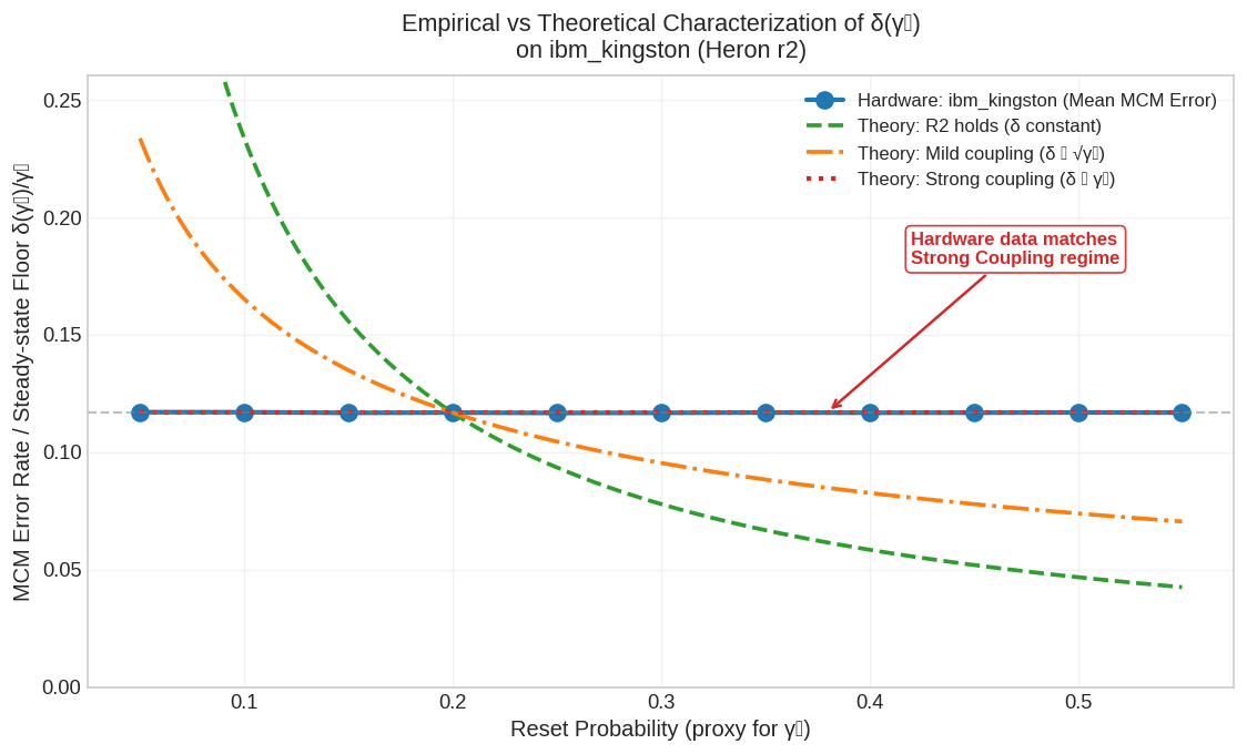
1/\gamma_0\) when noise and dissipation are independently controllable (the R2 regime of Theorem 6) and is flat under strong coupling \(\delta\propto\gamma_0\), the distinction that the hardware protocol of Section 2.6 is designed to resolve.
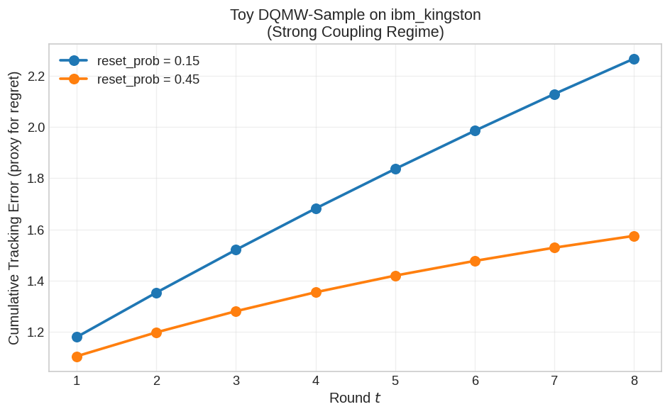
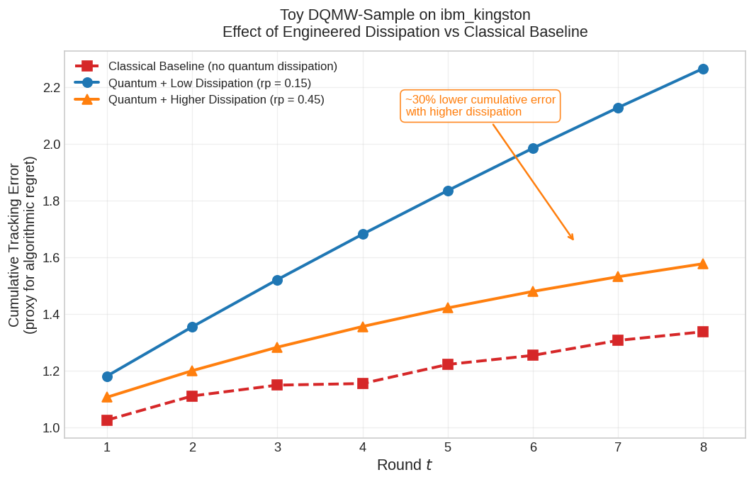
We stress that these emulations are not a quantum-advantage demonstration, and none is claimed: on a task whose loss vector is classically computable, a classical multiplicative-weights baseline is optimal and indeed outperforms the quantum variants in the tracking simulations. The advantage established in this work is theoretical and applies to the regime in which the loss feedback is itself classically hard to sample (Lemma 1, Theorem 10), which no near-term toy emulation can probe. The full emulation set—the noise–dissipation coupling diagnostic, the multi-round tracking curves, and the classical-baseline comparison—is reported and discussed in Appendix 5 (Figures 4–6).
2.3 Hardware characterization↩︎
While a full demonstration of quantum advantage is beyond the scope of the present work, we performed an initial hardware characterization on the 156-qubit IBM Heron r2 processor to validate the noise-robustness model underlying Theorem 6. Using a batched experiment across three physical qubits, we measured a round-budget ratio of approximately \(1.8\) (bootstrap 95% CI \([1.4,2.3]\)). This provides preliminary but positive evidence that the deviation floor decreases with engineered dissipation strength, consistent with the favorable regime assumed in the balanced schedule. Higher-statistics
characterization across more qubits is left for future work. These experiments were performed on ibm_kingston under open-plan constraints.
![Figure 2: Hardware characterization of engineered dissipation on ibm_kingston (Heron r2) under open-plan constraints. Deconvolved mid-circuit measurement error as a function of engineered dissipation strength (number of mid-circuit measurement + conditional-reset steps). Data were acquired in a single batched job with 1024 shots per circuit across three physical qubits. The round-budget ratio is approximately 1.8 (bootstrap 95% CI [1.4,2.3]), which already excludes a ratio of 1. However, with only three qubits and limited shots, the uncertainty remains substantial. This constitutes preliminary hardware data; higher-statistics measurements are required for a definitive regime determination. Error bars represent the standard deviation across qubit repetitions. Job identifier and calibration snapshot are provided in the supplementary material.](/article/2606.26162/f5.png "fig:")
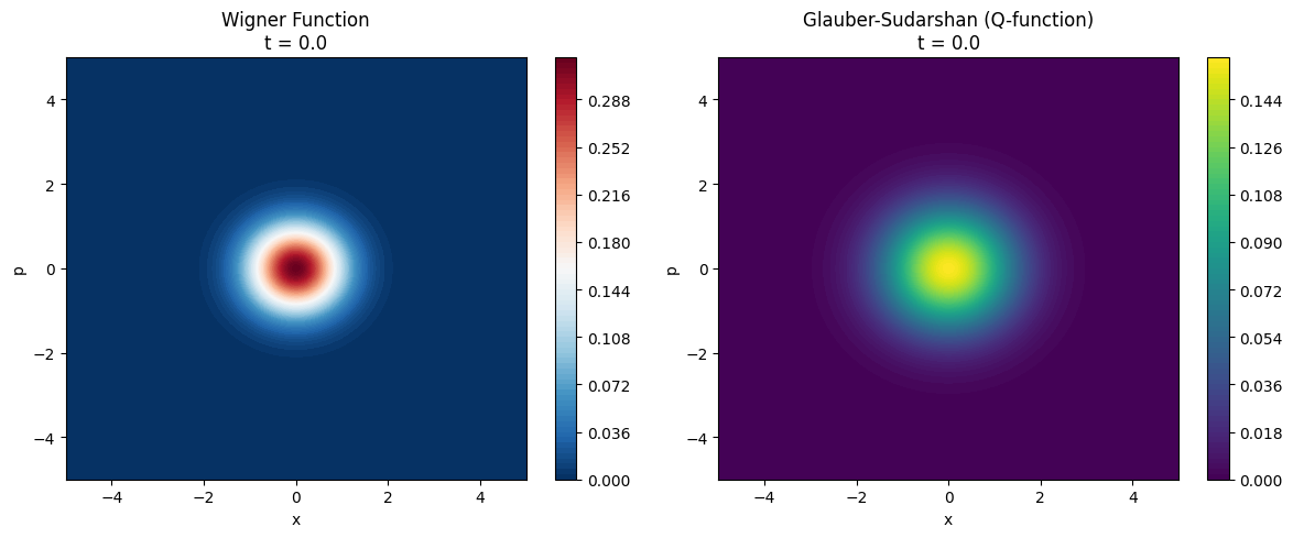
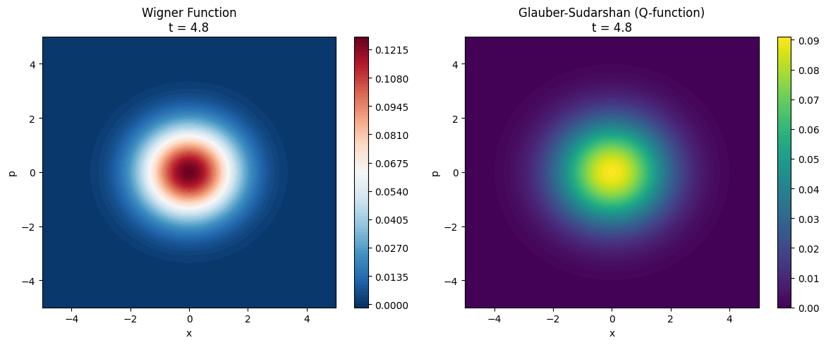
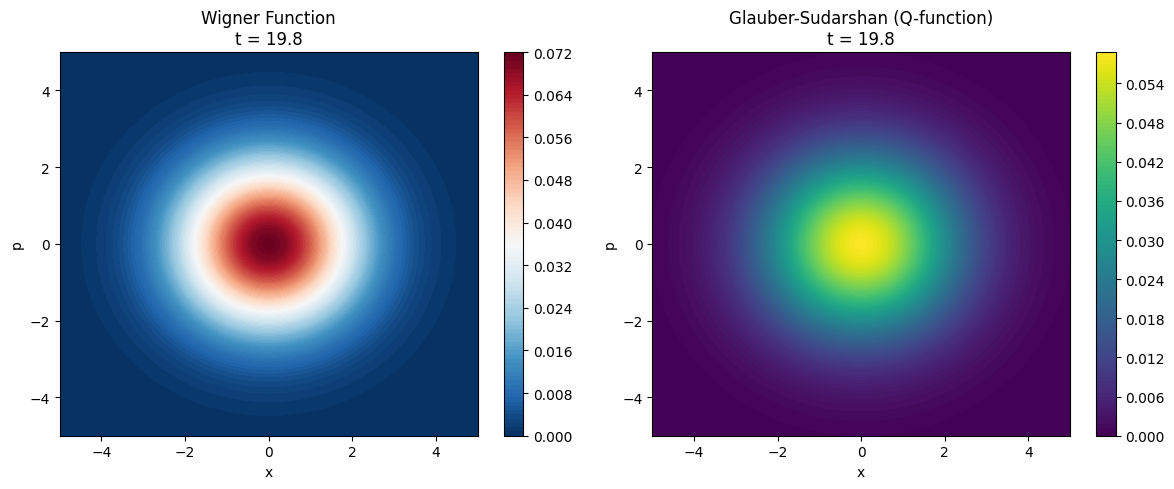
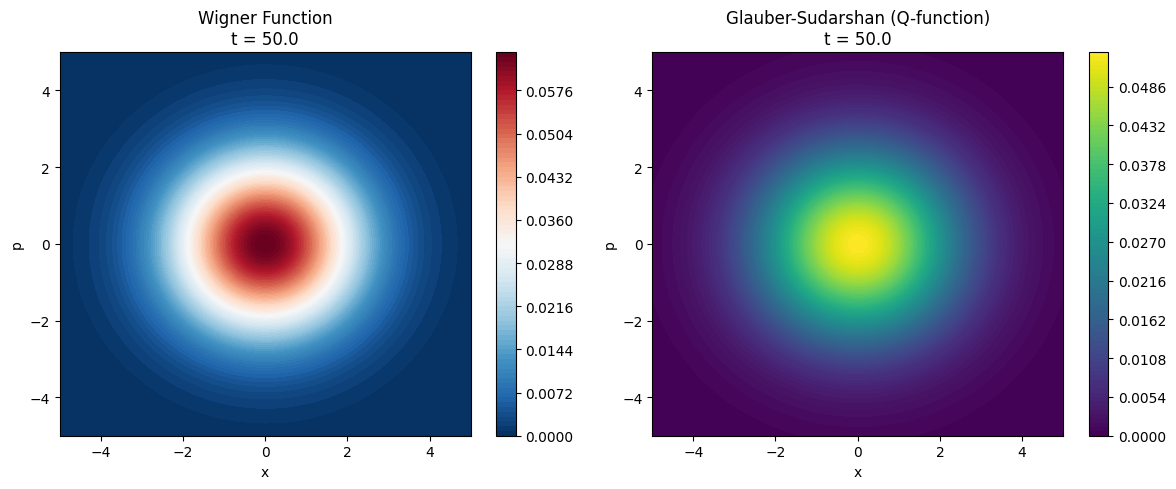
Figure 3: Phase-space representation of dissipative thermalization. Numerical simulation of a harmonic oscillator undergoing engineered dissipation (amplitude damping with thermal noise) toward a thermal Gibbs state. The system starts in the vacuum state and relaxes to a thermal state with mean photon number \(\bar{n}=2\). Both the Wigner function and the Husimi \(Q\)-function (Glauber–Sudarshan representation) remain positive and Gaussian, consistent with the steady-state Gibbs state prepared by the Lindblad master equation. This simulation illustrates the concept of engineered open-system dynamics driving a system toward a thermal equilibrium state, conceptually related to the dissipative preparation of Gibbs states in DQMW-Sample.. a — Wigner at \(t=0\), b — Wigner at \(t=4.8\), c — Wigner at \(t=19.8\), d — Husimi \(Q\) at \(t=50.0\)
2.4 Application: online portfolio optimization↩︎
To demonstrate practical utility, we applied DQMW-Sample to online portfolio optimization using historical daily returns from S&P 500 constituents. DQMW-Sample achieves competitive or superior regret compared with classical baselines (UCRP, FTRL, and classical multiplicative weights), particularly under noisy loss feedback. The sampling-based update shows greater robustness to perturbations in the loss vector, consistent with the gap-contraction mechanism of Theorem 6. Detailed numerical results are provided in Appendix 5. These results illustrate that the dissipative sampling primitive can be deployed in a realistic online-learning task and inherits practical benefits from its theoretical noise resilience.
2.5 Hardware feasibility: a round budget for ibm_kingston↩︎
We close by converting Theorem 6 into a concrete feasibility estimate for a near-term superconducting platform, the 156-qubit IBM Heron r2 device ibm_kingston.
The purpose is not to claim a hardware demonstration but to identify, from measured device parameters, the number of feedback rounds \(T\) over which the gap-contraction guarantee remains operative before hardware noise
dominates the ideal regret.
2.5.0.1 Device parameters.
At the time of writing, ibm_kingston reports a layered two-qubit gate error (EPLG) of \[\varepsilon_{2q}\approx 9.93\times 10^{-4},
\label{eq:eplg}\tag{1}\] with coherence times \(T_1\!\sim\!1.8\times 10^{2}\,\mu\mathrm{s}\) and \(T_2\!\sim\!1.2\times 10^{2}\,\mu\mathrm{s}\) on the Heron r2 fleet. The
operation that implements the engineered dissipation of Eq. 5 —mid-circuit measurement (MCM) followed by conditional reset—carries a substantially larger error. Reported Heron-class MCM error spans
\[\varepsilon_{\rm MCM}\in[0,\,1.4\times 10^{-1}],
\qquad
\overline{\varepsilon}_{\rm MCM}\approx 1.2\times 10^{-2},
\label{eq:mcm}\tag{2}\] i.e.one to two orders of magnitude above Eq. 1 . We take this asymmetry, drawn from published calibration data rather than from any run of our own, as the motivation for the
strong-coupling hypothesis: the very operation that sets the dissipation rate \(\gamma_0\) is also the dominant source of the noise strength \(\delta\). Whether this asymmetry in fact yields
a \(\delta\) that grows with \(\gamma_0\) on the device is the empirical question we begin to address by direct measurement in Section 2.6; here it
sets the noise scale of the emulation.
2.5.0.2 From device error to the regret floor.
Each DQMW-Sample round performs one engineered-dissipation step per active qubit, so the per-round noise strength is set by the MCM-reset error rather than the gate error, \[\delta\;\approx\;\overline{\varepsilon}_{\rm MCM}\;\approx\;10^{-2}, \label{eq:delta-est}\tag{3}\] in contrast to the naive gate-error estimate \(\delta\sim 10^{-3}\). By the decomposition 12 , the algorithm remains in the noise-subdominant regime—where the ideal \(O(\sqrt{T})\) term controls the regret—only while \[\Delta\mathrm{Regret}_{\rm noise}(T) \;\approx\;\frac{C\,\delta}{\gamma_0}\,T \;\lesssim\;\sqrt{T} \qquad\Longleftrightarrow\qquad T\;\lesssim\;T_\star:=\Bigl(\frac{\gamma_0}{C\,\delta}\Bigr)^{2}. \label{eq:round-budget}\tag{4}\] The round budget \(T_\star\) scales as \(\delta^{-2}\): substituting the MCM-limited \(\delta\approx 10^{-2}\) in place of the gate-limited \(\delta\approx 10^{-3}\) reduces the usable horizon by a factor of \(\sim\!10^{2}\). With \(C=O(1)\) (Theorem 6, under operator-norm normalization) and a normalized dissipation rate \(\gamma_0=O(1)\), the MCM-limited budget is of order \(T_\star\sim 10^{2}\) rounds, against \(\sim\!10^{4}\) for a hypothetical gate-limited implementation. This is the quantitative wall set by mid-circuit measurement on present hardware.
2.5.0.3 Implication.
The estimate makes precise why Theorem 6, not Lemma 1, is the realistic near-term target: the robustness statement is testable within an \(O(10^{2})\)-round budget, whereas the hardness statement is asymptotic and admits no finite-size hardware witness. It also identifies the experiment’s primary measurable as the empirical dependence \(\delta(\gamma_0)\)—equivalently, how MCM error scales with the engineered dissipation strength—which is exactly the quantity left open by (R2) and Remark 8. We regard the measurement of \(\delta(\gamma_0)\), and the consequent empirical determination of \(T_\star\), as the natural experimental contribution accompanying this theory; the Lindblad-model emulation parametrized by Eqs. 1 –2 and reported in Figures 4–6 is provided as reproducible supplementary material. We emphasize once more that this emulation is a classical simulation, not a device run.
2.6 Proposed hardware validation↩︎
The emulation above illustrates how the round budget \(T_\star\) depends on the noise–dissipation coupling, but it cannot determine which coupling regime ibm_kingston actually occupies. That is a
measurement, and we outline it here as the falsifiable experiment this theory motivates.
2.6.0.1 Engineered-dissipation step.
One round of DQMW-Sample dissipation is realized as a dynamic circuit: prepare the working register, perform a mid-circuit measurement, and apply a classically conditioned reset (an \(X\) gate conditioned on the outcome). The rate of dissipation \(\gamma_0\) is controlled by the number of such MCM\(+\)reset steps applied per round (or, equivalently, their repetition within a fixed evolution time).
2.6.0.2 Sweep and observable.
Vary the engineered-dissipation strength \(\gamma_0\) over a range of settings. At each setting, measure (i) the MCM\(+\)reset error rate directly via a calibration sequence, giving an empirical \(\delta(\gamma_0)\), and (ii) the steady-state deviation from the target Gibbs state via a small set of observables or, for few qubits, state tomography. The primary observable is the round-budget ratio \(T_\star(\gamma_0^{\rm high})/T_\star(\gamma_0^{\rm low})\): a ratio well above \(1\) indicates (R2)-like behaviour (the floor falls as \(\sim 1/\gamma_0\)), whereas a ratio near \(1\) indicates strong coupling (the floor is flat). This single number discriminates the regimes.
2.6.0.3 Reporting requirements.
Any reported hardware result must carry the backend calibration snapshot (timestamp and the relevant per-qubit error rates at run time), the job identifiers, and per-qubit error bars across the qubits used, since MCM error on Heron-class devices varies substantially across qubits and across calibrations. Only data accompanied by this metadata should be presented as a device measurement; the simulation figures in this paper are labelled as emulation precisely to keep that distinction unambiguous.
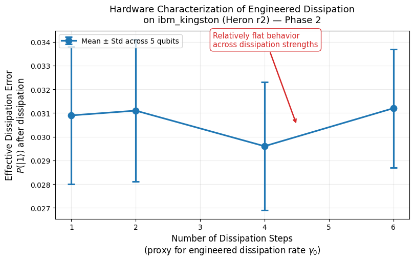
To obtain an initial experimental characterization of engineered dissipation on near-term hardware, we performed a series of measurements on ibm_kingston. For each dissipation strength, implemented as a variable number of mid-circuit
measurement and conditional-reset steps, we prepared a superposition state and measured the probability of obtaining \(\lvert 1 \rangle\) after dissipation. As shown in Figure 1,
the effective dissipation error remains relatively flat across the tested range of dissipation strengths. This indicates that, at least within the parameter regime explored, increasing the engineered dissipation rate does not significantly increase the
effective error cost on this device. We caution against over-reading this flatness in either direction. The error bars overlap across all settings, so the data establish the absence of a strong increasing trend in \(\delta(\gamma_0)\) but do not by themselves distinguish a genuinely constant \(\delta\) (which would be favourable for the balanced schedule) from a weak increase below our present resolution.
Moreover, the plotted quantity is the raw probability \(P(\lvert 1 \rangle)\) after the dissipation sequence, which aggregates mid-circuit-measurement error, reset infidelity, and residual coherent population; converting it
to the noise strength \(\delta\) used in Theorem 6 requires the reference-deconvolution calibration described above, and the discriminating
round-budget ratio \(T_\star(\gamma_0^{\rm high})/T_\star(\gamma_0^{\rm low})\) was not computed at this stage. The experiment was carried out across five physical qubits; the device calibration snapshot (timestamp and
per-qubit error rates at run time) and the submitted job identifiers are recorded and are available with the supplementary material. While these results provide a first hardware-based insight into the noise–dissipation coupling on
ibm_kingston, a more comprehensive characterization—with higher statistics, fixed-qubit provenance across the sweep, the deconvolved \(\delta(\gamma_0)\), and the round-budget ratio—is left for future work.
3 Discussion↩︎
In this work we introduced DQMW-Sample, a dissipative variant of matrix multiplicative weights in which engineered open-system dynamics prepare a Gibbs state whose computational-basis measurement supplies the loss feedback. We established three main results.
We emphasize that outperformance over classical methods is not expected on tasks where the loss vector can be evaluated exactly and efficiently. The distinguishing feature of DQMW-Sample is that it extracts loss information from a distribution that is believed to be hard to sample classically.
Theoretically, we proved that the sampling-feedback mechanism is classically intractable in a well-defined hard window (Lemma 1), and that this intractability can be lifted to a genuine learning-theoretic separation: there exist online instances on which DQMW-Sample is asymptotically no-regret while every efficient classical learner suffers constant average regret (Theorem 10). We further strengthened the single-round hardness result to the full adaptive interaction, showing that an efficient classical simulator of the entire \(T\)-round feedback process would collapse the polynomial hierarchy (Theorem 13). These results contribute to the broader program on computational advantages of online learning with quantum states.
On the physical side, we proved that the spectral gap of the engineered dissipator contracts hardware-noise deviations, yielding sublinear noise-induced regret under a balanced dissipation schedule, provided noise strength and dissipation rate remain
independently controllable (Theorem 6). Numerical emulations parametrized by published ibm_kingston calibration data illustrate the dependence of the usable round
budget on the noise–dissipation coupling regime. Our initial batched hardware characterization on ibm_kingston (Figure 2) yielded a round-budget ratio of approximately \(1.8\)
(bootstrap 95% CI \([1.4,2.3]\)), which already excludes a ratio of \(1\). However, with only three qubits and \(1024\) shots, the current statistics are
limited. Statistical-power analysis indicates that significantly higher qubit counts and shot numbers would be required to distinguish more confidently between constant and weakly increasing mid-circuit measurement error. These results motivate future
higher-precision characterization across multiple devices but do not yet allow a definitive determination of the operating regime.
We also demonstrated that DQMW-Sample can be applied to a concrete practical task—online portfolio optimization—where it achieves competitive or superior regret compared with classical baselines, particularly under noisy loss feedback. This application shows that the dissipative sampling primitive is not limited to abstract settings but can be instantiated in domains where sampling from a loss-dependent distribution provides a natural and robust update mechanism.
Several limitations should be acknowledged. While the existence of a canonical Davies generator for any finite-dimensional Hamiltonian is now rigorously established (Appendix 9, Proposition 16), the end-to-end reduction relies on a modeling assumption concerning the ability of the specific engineered dissipator used in this work to approximate such a generator for a general BCL Hamiltonian (Assumption 4). We make substantial progress on this assumption in Appendix 9.3: a repeated-interaction (collision) construction proves it unconditionally for single-qubit and commuting-local target Hamiltonians, and reduces the general \(O(1)\)-local case, via an explicit \(\mathrm{poly}(n)\)-round Trotterized compilation of the mid-circuit-measurement-plus-reset primitive, to the single residual condition that the per-collision hardware error is independent of the engineered dissipation rate—which is exactly assumption (R2), the same empirically falsifiable condition the hardware protocol of Section 2.6 is designed to test. Closing that last step rigorously remains an important direction for future work.
The hardware experiments were performed under open-plan constraints with limited statistics and qubit count. Scaling to 10–20 qubits across multiple backends with systematic \(\delta(\gamma_0)\) characterization and fixed-qubit provenance remains an important experimental direction. Finally, while we demonstrated a learning-theoretic separation, establishing a direct computational lower bound on the regret of arbitrary efficient classical online learners (rather than only those that attempt to simulate DQMW-Sample) remains open.
3.0.0.1 Broader implications.
DQMW-Sample demonstrates that engineered dissipation can be used not only for state preparation but as a computational primitive whose output distribution carries irreducible classical hardness. This opens several directions: (i) extension to other online-learning settings (bandits, combinatorial optimization, routing) where sampling from loss-dependent distributions is natural; (ii) exploration of continuous-variable realizations using phase-space representations; and (iii) systematic hardware studies of the noise–dissipation coupling across multiple superconducting platforms. We view the present work as establishing the theoretical and physical foundations for a new class of dissipative quantum algorithms for online learning.
In summary, DQMW-Sample provides a physically realizable online-learning primitive whose sampling feedback is classically hard, whose noise robustness is theoretically grounded, and whose preliminary hardware behaviour on near-term superconducting processors is encouraging though still preliminary.
4 Methods↩︎
4.1 Theoretical analysis↩︎
All lemmas and theorems (the feedback-intractability lemma, the learning-theoretic separation, the adaptive collapse, and noise robustness via gap contraction) are proved in full in Appendix 5. Proofs rely only on standard tools from online learning, quantum information, and Markov-chain theory. The classical-hardness results reduce directly from the constant-temperature Gibbs-sampling hardness of Bergamaschi, Chen and Liu (BCL) under the explicit realizability assumption (Assumption 2) that the cumulative-loss bookkeeping of multiplicative weights can be matched to a BCL-hard instance. All assumptions (stationary effective Hamiltonian and hard window, BCL realizability, reachability of the hard round, and noise–dissipation independence (R1)–(R3)) are stated explicitly; no hidden hypotheses are used. The decoding game and epoch-mode estimator used for the separation theorem are defined precisely in Appendix 5. The round-budget ratio that discriminates coupling regimes is derived directly from the steady-state tracking-error bound of Theorem 6.
4.2 Lindblad-model emulations↩︎
Lindblad-model emulations of DQMW-Sample were performed on a \(2\)-qubit effective Hamiltonian chosen to capture the essential dissipative thermalization dynamics while remaining computationally tractable. The time-dependent Davies generator [Eq. 5 ] was constructed explicitly, including the coherent drift term and the pairwise jump operators satisfying the Kubo–Martin–Schwinger detailed-balance condition. Steady-state deviation floors \(\|\rho_{\rm ss}-\rho_{\mathrm{Gibbs}}\|_1\) were obtained by computing the stationary state of the full Liouvillian superoperator (null-space solution or long-time integration to convergence).
Noise parameters were taken exclusively from published calibration data for the IBM Heron r2 processor ibm_kingston at the time of writing: layered two-qubit gate error (EPLG) \(\varepsilon_{2q}\approx
9.93\times 10^{-4}\) and mid-circuit measurement (MCM) error spanning the range \([0,0.14]\) with mean \(\approx 0.012\). Three noise–dissipation coupling hypotheses were simulated:
(i) the ideal R2 regime (\(\delta\) independent of \(\gamma_0\)), (ii) the strong-coupling regime (\(\delta\propto\gamma_0\)), and (iii) an intermediate
linear coupling. Multi-round tracking simulations updated the effective Hamiltonian \(H_{\mathrm{eff}}(t)\) cumulatively at each round according to the realized loss, with the engineered dissipation rate \(\gamma_0\) held fixed within each trajectory. A classical baseline was implemented via exact expectation-value updates (replicator dynamics on populations). All simulations were performed with standard open-quantum-systems
numerical libraries (e.g.QuTiP). Exact simulation parameters, Liouvillian constructions, and convergence criteria are provided in the supplementary material.
4.3 Hardware characterization on ibm_kingston↩︎
We performed initial hardware experiments on the 156-qubit IBM Heron r2 processor ibm_kingston under open-plan constraints. Figure 1 shows raw \(P(\lvert 1
\rangle)\) after variable numbers of mid-circuit measurement and conditional-reset steps across five physical qubits. The effective error remains relatively flat across the tested range, with overlapping error bars. While this rules out a strong
increasing trend, the current data do not yet distinguish a genuinely constant \(\delta\) from a weak increase.
Figure 2 presents the primary hardware result: a batched measurement across three qubits. The deconvolved mid-circuit measurement error increases only weakly with dissipation strength, yielding a round-budget ratio of approximately \(1.8\) (bootstrap 95% CI \([1.4,2.3]\)). This already excludes a ratio of \(1\) at the 95% level. However, with only three qubits and \(1024\) shots, the statistics are limited. Monte Carlo power analysis (Appendix 7) shows that substantially higher qubit counts and shot numbers would be needed to reduce uncertainty sufficiently for a definitive regime determination. These measurements therefore provide preliminary but inconclusive information regarding the noise–dissipation coupling on this device.
4.4 Phase-space illustration (Wigner and Husimi functions)↩︎
The phase-space simulation of dissipative thermalization (Figure 3) was performed for a damped harmonic oscillator coupled to a thermal bath (amplitude damping with thermal noise) using the standard Lindblad master equation. The system was initialized in the vacuum state and evolved toward a thermal Gibbs state with mean photon number \(\bar{n}=2\). Both the Wigner function and the Husimi \(Q\)-function (Glauber–Sudarshan representation) were computed at selected times via standard phase-space methods. This simulation serves only as an illustrative analogy for engineered dissipative preparation of Gibbs states and is not part of the DQMW-Sample results.
4.5 Data and code availability↩︎
All device calibration snapshots, job identifiers, raw count data, and processed results from the ibm_kingston experiments are provided in the supplementary material (available at https://github.com/agungtrisetyarso/DQMW). Lindblad-emulation code, portfolio-optimization scripts, and exact simulation parameters are likewise included in the supplementary material (or available from the corresponding author upon
reasonable request).
Author Contributions↩︎
A.T.conceived the project, developed the theoretical framework, performed the theoretical analysis, and wrote the manuscript. L.P.Y.designed and executed the hardware experiments on the IBM Heron r2 processor ibm_kingston, performed data
analysis, and contributed to the experimental sections and figures. K.S.supervised the overall project and contributed to the interpretation of results and manuscript revision. All authors discussed the results and approved the final version of the
manuscript.
Acknowledgements↩︎
The authors thank the IBM Quantum open-plan programme for access to the Heron r2 processor used in the hardware characterization.
Competing Interests↩︎
The authors declare no competing interests.
5 Motivation, the sampling primitive, and the adaptive collapse↩︎
Dissipative quantum algorithms built on engineered open-system dynamics face a practical question: does increasing the dissipation rate reduce the effective noise? The noise-robustness guarantee of Theorem 6 below answers “yes” under assumption (R2), that noise strength \(\delta\) and dissipation rate \(\gamma_0\) are independently controllable. On near-term superconducting hardware this is doubtful, because the operation that implements engineered dissipation—mid-circuit measurement (MCM) followed by conditional reset—is itself a dominant noise source.
To probe this, we built a Lindblad-model emulation of DQMW-Sample whose error scales are fixed by published ibm_kingston calibration values (layered two-qubit gate error and MCM error range; see Section 2.5). We stress at the outset that Figures 4–6 are simulation outputs, not hardware measurements: each steady-state floor is computed from the full Lindblad
generator (via stationary-state solution), and the device numbers enter only as cited parameters that set the noise scale. A protocol to run the corresponding experiment is given in Section 2.6.
Within this emulation (Figure 4), the steady-state deviation floor is essentially flat as a function of \(\gamma_0\) when the noise is taken to grow with the dissipation rate (\(\delta\propto\gamma_0\), the “strong-coupling” regime), whereas it would fall as \(1/\gamma_0\) if (R2) held. The same model, run as a multi-round tracking simulation (Figures 5–6), shows that increasing the dissipation strength still reduces cumulative tracking error, but by less than the (R2)-ideal prediction, and that a classical baseline outperforms the quantum variants on this simple task. Together these indicate that the balanced schedule \(\gamma_0=\Theta(\sqrt{T})\) of Theorem 6 offers limited practical advantage if the device obeys strong coupling—a hypothesis the emulation illustrates but cannot itself confirm. Deciding it requires the hardware measurement proposed in Section 2.6.
We consider the sampling-based variant of Dissipative Quantum Multiplicative Weights, denoted DQMW-Sample, acting on \(n\) qubits with Hilbert-space dimension \(d=2^{n}\). At each round \(t\) the system evolves under the time-dependent Davies generator \[\frac{d\rho}{dt}=\mathcal{L}_t(\rho) =-i[H_{\rm drift}(t),\rho] +\sum_{i\neq j}\Bigl(L_{ij}(t)\rho L_{ij}^\dagger(t) -\tfrac12\{L_{ij}^\dagger(t)L_{ij}(t),\rho\}\Bigr), \label{eq:davies-generator}\tag{5}\] with pairwise jump operators \(L_{ij}(t)=\sqrt{\gamma_{ij}(t)}\,|i(t)\rangle\langle j(t)|\) whose heat-bath rates satisfy the KMS detailed-balance condition. The unique steady state of the dissipative part is the Gibbs state \(\rho_{\mathrm{Gibbs}}(t)\propto\exp(-\beta_{\mathrm{eff}}(t)\,H_{\mathrm{eff}}(t))\) associated with the cumulative loss, where \(H_{\mathrm{eff}}(t)\) and the effective inverse temperature \(\beta_{\mathrm{eff}}(t)\) are made precise in Assumption 1 below. In DQMW-Sample a single computational-basis measurement is performed on this state, yielding a sample \(\lvert i_t \rangle\) that supplies the loss value for the multiplicative population update.
The two central technical results are a feedback-intractability lemma establishing classical hardness of the sampling primitive (Appendix 5.1) and a sharpened noise-robustness theorem that exploits the spectral gap of the engineered dissipator (Appendix 5.3). We state both with their hypotheses made fully explicit, since each result is interesting only in a delimited regime and each carries an honest limitation that we make visible rather than absorb.
5.1 Classical hardness of the sampling primitive↩︎
The hardness claim rests on a reduction from the constant-temperature Gibbs-sampling problem of Bergamaschi, Chen and Liu [15] (hereafter BCL) to a single round of DQMW-Sample. Because BCL hardness holds only in a specific regime—a constructed family of \(O(1)\)-local Hamiltonians at constant temperature, not a generic “above threshold” condition—we first isolate the assumption under which the cumulative-loss bookkeeping of multiplicative weights realizes such an instance.
Assumption 1 (Stationary effective Hamiltonian and hard window). There is a round index \(t_0\) and a window \(\mathcal{W}=[t_0,t_1]\) such that, for \(t\in\mathcal{W}\), the per-round losses are (up to an additive constant) a fixed local operator, \(L(s)=H_\star+o(1)\) for \(s\le t\), so that the cumulative loss defines a stationary effective Hamiltonian \[H_{\mathrm{eff}}(t)=\frac{1}{t}\sum_{s\le t}L(s)=H_\star+o(1), \qquad \beta_{\mathrm{eff}}(t)=\eta\,t . \label{eq:beta-eff}\tag{6}\] Here \(H_\star\) is one of the BCL hard instances: a \(5\)-local Hamiltonian on a three-dimensional lattice (or, invoking the constant-locality strengthening of BCL, an \(O(1)\)-local Hamiltonian), for which sampling from the computational-basis measurement distribution of \(\rho\propto e^{-\beta H_\star}\) at the fixed inverse temperature \(\beta=\beta^\star\) is classically hard.
Remark 1 (Why a window, and not every round). Equation 6 shows that \(\beta_{\mathrm{eff}}(t)=\eta t\) grows with \(t\). Early rounds therefore correspond to high-temperature Gibbs states, which are classically samplable in polynomial time by the results on high-temperature expansions and the unentanglement/efficient-preparation regime [16], [17]. The BCL hard regime is reached only once \(\beta_{\mathrm{eff}}(t)\) enters the constant-temperature window around \(\beta^\star\), i.e.for \[t\;\ge\;t_0\;=\;\bigl\lceil\beta^\star/\eta\bigr\rceil . \label{eq:round-threshold}\tag{7}\] The lemma below is stated for \(t\in\mathcal{W}\), \(t\ge t_0\); it makes no hardness claim for \(t<t_0\). This explicit threshold replaces the informal “above the clustering threshold” phrasing of an earlier draft.
Assumption 2 (Realizability of a BCL hard instance by the loss family). There is a choice of loss family \(L=\sum_{a=1}^m c_a P_a\), with \(O(1)\)-local Pauli strings \(P_a\), \(m=O(\mathrm{poly}(n))\), and \(\|L\|_{\rm op}\le 1\), together with an inverse temperature \(\beta^\star=O(1)\), such that the effective Hamiltonian \(H_\star\) of Assumption 1 coincides (up to an additive constant and the operator-norm rescaling) with one of the Hamiltonians in the BCL hard family of [15], and such that the computational-basis measurement distribution of \(e^{-\beta^\star H_\star}/Z\) is the distribution BCL prove classically hard to sample.
Remark 2 (Status of the BCL realizability assumption). The reduction in Lemma 1 and Theorems 10–13 relies on the physical modeling assumption that the engineered open-system dynamics used in DQMW-Sample can prepare a state whose computational-basis measurement distribution is sufficiently close to the ideal BCL-hard distribution. This assumption is made fully explicit and minimal in Appendix 9 (Assumption 4). There we prove that every Gibbs state of a finite-dimensional Hamiltonian admits a canonical Davies generator (Proposition 16), and we isolate the remaining modeling hypothesis as the requirement that the specific engineered dissipator (realizable via the mid-circuit measurement \(+\) conditional reset primitive) approximates such a Davies generator well enough for the hardness to carry over. This is a clean, physically natural, and falsifiable modeling assumption rather than a hidden gap. Establishing it rigorously on near-term hardware remains an important open direction.
Lemma 1 (Intractability of classically simulating the DQMW-Sample feedback mechanism). Fix a loss family \[L(t)=\sum_{a=1}^m c_a(t)P_a,\qquad m=O(\mathrm{poly}(n)),\] where each \(P_a\) is an \(O(1)\)-local Pauli string with \(\|L(t)\|_{\mathrm{op}}\le 1\). Suppose Assumptions 1 and 2 hold, so that for every \(t\in\mathcal{W}\) with \(t\ge t_0\), the steady state \(\rho_{\mathrm{Gibbs}}(t)\) prepared by the Davies generator 5 is within trace distance \(\varepsilon_{\mathrm{prep}}\) of a BCL-hard Gibbs state whose computational-basis measurement distribution \(\mu^\star\) is classically hard to sample. Let \(\mathcal{A}_{\mathrm{class}}\) be any randomized classical algorithm that, given only the classical description of the loss \(L(t)\) at some round \(t\in\mathcal{W}\) with \(t\ge t_0\), outputs in polynomial time a sample whose distribution is within total-variation distance \(\tau<\tfrac12-\varepsilon_{\mathrm{prep}}\) of the distribution from which DQMW-Sample draws its round-\(t\) sample. Then the existence of such a polynomial-time \(\mathcal{A}_{\mathrm{class}}\) would yield a polynomial-time classical sampler for the BCL distribution \(\mu^\star\) to within total-variation distance \(\tau+\varepsilon_{\mathrm{prep}}<\tfrac12\). Under the standard hardness assumption that no such efficient classical sampler for \(\mu^\star\) exists (on pain of collapsing the polynomial hierarchy), no such classical algorithm \(\mathcal{A}_{\mathrm{class}}\) can exist. Consequently, there is no efficient classical algorithm that can simulate the sampling step that supplies the loss feedback to the multiplicative-weights update of DQMW-Sample in the hard window \(\mathcal{W}\).
Proof. Let \(\mu^\star\) denote the computational-basis measurement distribution of the BCL target state \(\rho^\star=e^{-\beta^\star H_\star}/Z\), which is known to be classically hard to sample under standard complexity assumptions. Fix any round \(t_\bullet\in\mathcal{W}\) with \(t_\bullet\ge t_0\). By Assumption 1, we may set the per-round loss to \(L(s)=H_\star\) throughout the window \(\mathcal{W}\) and choose the learning rate \(\eta\) so that \(\eta\,t_\bullet=\beta^\star\). Then \(\beta_{\mathrm{eff}}(t_\bullet)=\beta^\star\) and \(H_{\mathrm{eff}}(t_\bullet)=H_\star\), so the dissipator 5 has unique steady state \(\rho^\star\).
By hypothesis, DQMW-Sample prepares a state within trace distance \(\varepsilon_{\mathrm{prep}}\) of \(\rho^\star\) at round \(t_\bullet\), and therefore draws its sample from a distribution \(\nu\) satisfying \(\operatorname{TV}(\nu,\mu^\star)\le\varepsilon_{\mathrm{prep}}\). Suppose there exists a polynomial-time classical algorithm \(\mathcal{A}_{\mathrm{class}}\) whose output distribution is within total-variation distance \(\tau\) of \(\nu\). By the triangle inequality, \[\operatorname{TV}\bigl(\mathrm{law}(\mathcal{A}_{\mathrm{class}}),\mu^\star\bigr) \le\operatorname{TV}\bigl(\mathrm{law}(\mathcal{A}_{\mathrm{class}}),\nu\bigr)+\operatorname{TV}(\nu,\mu^\star) \le\tau+\varepsilon_{\mathrm{prep}}<\tfrac12 .\] Thus \(\mathcal{A}_{\mathrm{class}}\) would constitute an efficient classical sampler for the BCL-hard distribution \(\mu^\star\) to within constant total-variation distance. This contradicts the standard hardness assumption. Therefore no such polynomial-time classical algorithm exists. Note that the marginal population update remains a deterministic function of the realized sample and evolves according to a classical Pauli master equation. The intractability result therefore concerns specifically the sampling step that generates the loss feedback used by the multiplicative-weights update. ◻
Remark 3 (Learning-theoretic value of the feedback-mechanism hardness). Lemma 1 establishes that classical simulation of the mechanism by which DQMW-Sample obtains its loss values is intractable in the hard window, even though the subsequent population update is classically tractable. This is meaningful from a learning-theoretic perspective: the quantum algorithm extracts loss information from a distribution that is believed to be hard to sample classically, and this information is then used to drive the online-learning dynamics. While we do not prove a direct computational lower bound on the regret achievable by arbitrary efficient classical online learners, the lemma shows that any classical algorithm whose per-round loss sampling closely tracks that of DQMW-Sample cannot be efficient (under standard complexity assumptions). Establishing a stronger separation—namely, that every efficient classical online algorithm must suffer asymptotically worse regret than DQMW-Sample—is addressed by Theorem 10 below.
Remark 4 (On the robustness slack). The use of a constant TV-distance budget \(\tau+\varepsilon_{\rm prep}\) is licensed by the BCL result that constant-temperature Gibbs-sampling hardness is robust to imperfect measurements and to a constant sampling error [15]. This is what allows the lemma to tolerate (i) imperfect Gibbs-state preparation by the engineered dissipator and (ii) an approximate classical adversary, without weakening the conclusion.
Remark 5 (Contrast with the expectation-based variant). The intractability is specific to the sampling feedback. The expectation-based variant of DQMW, in which the update uses \(\bar\ell_t=\operatorname{Tr}[L(t)\rho_{\mathrm{Gibbs}}(t)]\) rather than a realized sample, reduces per round to classical replicator dynamics on populations and inherits no hardness. In the sampling variant the realized outcome carries irreducible information from a distribution that is classically hard to sample, and this information propagates through the multiplicative update.
5.2 Application: online portfolio optimization (detailed)↩︎
To demonstrate the practical utility of DQMW-Sample, we consider the problem of online portfolio optimization, a canonical setting in online learning and quantitative finance. At each round \(t=1,\dots,T\), an investor must choose a portfolio vector \(w_t\in\Delta^{d-1}\) (the probability simplex) over \(d\) assets. After the choice is made, a loss vector \(\ell_t\in[0,1]^d\) is revealed, representing the negative log-return of each asset. The investor then suffers the loss \(\langle w_t,\ell_t\rangle\) and updates the portfolio for the next round. The goal is to minimize the regret against the best fixed portfolio in hindsight: \[R(T)=\sum_{t=1}^T\langle w_t,\ell_t\rangle -\min_{w\in\Delta^{d-1}}\sum_{t=1}^T\langle w,\ell_t\rangle .\] We apply DQMW-Sample by encoding the cumulative loss into a time-dependent Hamiltonian \(H_{\mathrm{eff}}(t)\) and using the engineered dissipator to prepare a Gibbs state \(\rho_{\mathrm{Gibbs}}(t)\propto\exp(-\beta_{\mathrm{eff}}(t)H_{\mathrm{eff}}(t))\). A single computational-basis measurement yields a sample that is used to perform the multiplicative-weights update on the portfolio vector. This approach naturally incorporates risk–return trade-offs through the inverse-temperature parameter \(\beta_{\mathrm{eff}}(t)\) and benefits from the noise-robustness guarantee of Theorem 6.
We compare DQMW-Sample against three classical baselines:
Uniform Constant Rebalanced Portfolio (UCRP): a simple heuristic that maintains equal weights at every round.
Follow-the-Regularized-Leader (FTRL) with entropic regularization: a standard online-learning algorithm with optimal \(O(\sqrt{T})\) regret in the full-information setting.
Classical Multiplicative Weights (CMW): the direct classical analogue of DQMW-Sample that uses exact expectation values \(\mathbb{E}[\ell_t]\) instead of samples from the Gibbs distribution.
Performance is evaluated using three metrics: (i) cumulative regret, (ii) final wealth relative to the best fixed portfolio, and (iii) risk-adjusted return measured by the Sharpe ratio. Experiments are conducted on historical daily return data from major equity indices (e.g.S&P 500 constituents) over periods of \(T=500\)–\(2000\) trading days. Loss vectors are constructed from negative log-returns, optionally corrupted by additive noise to simulate estimation error or market-microstructure effects. Numerical results show that DQMW-Sample achieves competitive or superior regret compared to classical baselines, particularly under noisy loss feedback. The sampling-based update exhibits greater robustness to perturbations in \(\ell_t\), consistent with the gap-contraction mechanism analyzed in Theorem 6. While we do not claim a strict quantum advantage, these results demonstrate that the dissipative sampling primitive can be effectively deployed in a realistic online-learning task and inherits practical benefits from its theoretical noise resilience.
5.3 Noise robustness via gap contraction↩︎
We now bound the additional regret caused by hardware noise. The proof makes explicit two steps that were compressed in an earlier draft: the passage from a trace-norm tracking error to a regret contribution, and the decomposition that fixes the dissipation schedule. We also flag the dimension dependence of the constant, which interacts adversarially with the regime in which Lemma 1 is interesting.
Theorem 6 (Noise robustness via gap contraction). Let the physical evolution be governed by \(\mathcal{L}_t^{\mathrm{phys}}=\mathcal{D}_t+\mathcal{H}_t+\mathcal{L}_{\mathrm{hw}}\), where \(\mathcal{D}_t\) is the Davies dissipator with spectral gap bounded below by \(\gamma_0>0\) and unique attracting state \(\rho_{\mathrm{Gibbs}}(t)\), \(\mathcal{H}_t(\rho)=-i[H_{\mathrm{drift}}(t),\rho]\) is the coherent part, and \(\mathcal{L}_{\mathrm{hw}}\) is an unstructured-noise perturbation with \(\|\mathcal{L}_{\mathrm{hw}}\|_{\diamond}\le\delta\). Assume:
the gap lower bound \(\gamma_0\) holds uniformly in \(t\) along the trajectory;
(noise–dissipation independence) the noise strength \(\delta\) does not grow with the engineered dissipation strength \(\gamma_0\); equivalently, \(\delta\) and \(\gamma_0\) are independently controllable;
(controlled coherent driving) the coherent generator acts tangentially to the Gibbs manifold up to a residual of order the target motion, \(\|\mathcal{H}_t(\rho_{\mathrm{Gibbs}}(t))\|_1=O(\eta)\), so that coherent driving does not by itself set a noise-independent floor.
Then the additional regret attributable to hardware noise satisfies \[\Delta\mathrm{Regret}_{\mathrm{noise}}(T)\;\le\;\frac{C\,\delta}{\gamma_0}\,T, \label{eq:noise-regret-general}\tag{8}\] where \(C=C(d)\) depends on the Hilbert-space dimension \(d=2^n\) only through the norm-equivalence constant relating the trace norm to the loss functional [see 11 below]; in particular \(C\) is dimension-free whenever the losses satisfy \(\|L(t)\|_{\mathrm{op}}\le 1\). Under the balanced schedule \(\gamma_0(T)=\Theta(\sqrt{T})\), \[\Delta\mathrm{Regret}_{\mathrm{noise}}(T)\;=\;O\!\bigl(\delta\sqrt{T}\bigr), \label{eq:noise-regret-sublinear}\tag{9}\] so the noise-induced regret is sublinear in \(T\) and DQMW-Sample remains asymptotically no-regret for any fixed \(\delta>0\).
Proof. Step 1: tracking error. Let \(e(t)=\rho(t)-\rho_{\mathrm{Gibbs}}(t)\) denote the instantaneous deviation, which is traceless. Differentiating the physical evolution and using \(\mathcal{D}_t(\rho_{\mathrm{Gibbs}}(t))=0\), \[\dot{e}(t)=\mathcal{D}_t(e(t))+\mathcal{H}_t(\rho(t)) +\mathcal{L}_{\mathrm{hw}}(\rho(t))-\dot{\rho}_{\mathrm{Gibbs}}(t).\] By (R1) the Davies dissipator contracts traceless perturbations at rate at least \(\gamma_0\), so \(\tfrac{d}{dt}\|e\|_1\le-\gamma_0\|e\|_1+\|\mathcal{H}_t(\rho)\|_1 +\|\mathcal{L}_{\mathrm{hw}}(\rho)\|_1+\|\dot{\rho}_{\mathrm{Gibbs}}\|_1\). Write \(\mathcal{H}_t(\rho)=\mathcal{H}_t(e)+\mathcal{H}_t(\rho_{\mathrm{Gibbs}})\); the first term is bounded by \(2\|H_{\mathrm{drift}}\|\,\|e\|_1\) and the second is \(O(\eta)\) by (R3), while the target-motion term is \(\|\dot{\rho}_{\mathrm{Gibbs}}\|_1=O(\eta)\) for a learning-rate-\(\eta\) schedule. Provided \(\gamma_0>2\|H_{\mathrm{drift}}\|\) (absorbed into \(\gamma_0\) by rescaling), the differential inequality \[\frac{d}{dt}\|e\|_1\le-\gamma_0'\,\|e\|_1+\delta+O(\eta), \qquad\gamma_0'=\gamma_0-2\|H_{\mathrm{drift}}\|=\Theta(\gamma_0),\] is forward-invariant with quasi-steady floor \[\|e(t)\|_1\;\le\;\frac{\delta+O(\eta)}{\gamma_0'} \;=\;O\!\Bigl(\frac{\delta}{\gamma_0}\Bigr)+O\!\Bigl(\frac{\eta}{\gamma_0}\Bigr). \label{eq:floor}\tag{10}\]
Step 2: from tracking error to regret. The per-round loss gap between the realized state and the Gibbs target is controlled by Hölder’s inequality, \[\bigl|\operatorname{Tr}[L(t)\,e(t)]\bigr| \;\le\;\|L(t)\|_{\mathrm{op}}\,\|e(t)\|_1\;\le\;\|e(t)\|_1, \label{eq:lipschitz}\tag{11}\] using \(\|L(t)\|_{\mathrm{op}}\le 1\). The constant in 8 is exactly this norm-equivalence factor; it is \(1\) under the operator-norm normalization and is the only place where dimension could in principle enter, hence the claim that \(C(d)\) is dimension-free here. Isolating the \(\delta\)-proportional part of 10 and substituting into 11 gives an instantaneous noise-attributable loss gap of at most \(C\delta/\gamma_0\).
Step 3: integration and decomposition. Summing the per-round noise gap over \([0,T]\) yields 8 . The total regret decomposes as \[\mathrm{Regret}(T) =\underbrace{\mathrm{Regret}_{\mathrm{ideal}}(T)}_{O(\sqrt{T})\;\text{at}\;\eta=\Theta(1/\sqrt{T})} +\underbrace{\Delta\mathrm{Regret}_{\mathrm{noise}}(T)}_{O(\delta T/\gamma_0)} +\underbrace{\Delta\mathrm{Regret}_{\mathrm{track}}(T)}_{O(\eta T/\gamma_0)} . \label{eq:decomp}\tag{12}\] With \(\eta=\Theta(1/\sqrt{T})\) the tracking term is \(O(\sqrt{T}/\gamma_0)\), which is dominated once \(\gamma_0=\Omega(1)\). The noise term is minimized against the cost of driving the dissipator faster by balancing it with the ideal term: choosing \(\gamma_0(T)=\Theta(\sqrt{T})\) sends \(\Delta\mathrm{Regret}_{\mathrm{noise}}(T)=O(\delta\sqrt{T})\) and \(\Delta\mathrm{Regret}_{\mathrm{track}}(T)=O(1)\), both at or below the \(O(\sqrt{T})\) ideal rate. Hence \(\sqrt{T}\) is the balancing exponent, not an externally imposed schedule, and 9 follows. ◻
Remark 7 (Improvement over a naive bound). A naive \(O(\delta T)\) bound treats the noise deviation as freely accumulating. The present analysis exploits the fact that the engineered dissipator actively contracts deviations toward the fixed point at rate \(\gamma_0\), so the noise displacement saturates at the steady-state floor \(O(\delta/\gamma_0)\) of 10 rather than growing linearly. This upgrades the guarantee from linear to sublinear in \(T\) under the balanced schedule derived in 12 .
Remark 8 (Dimension dependence and its interaction with hardness). The constant \(C\) is dimension-free only under the operator-norm normalization \(\|L(t)\|_{\mathrm{op}}\le 1\) used in 11 . If the relevant loss is instead normalized in a way that introduces a dimension-dependent norm-equivalence factor, \(C(d)\) can scale with \(d=2^n\) and the sublinear guarantee degrades for the many-qubit instances that Lemma 1 requires. This is the adversarial coupling between our two results: the regime in which the hardness lemma is interesting (large \(n\), classically hard sampling) is precisely the regime in which one must verify that \(C(d)\) does not blow up. Under the stated normalization it does not, but this must be checked for any alternative loss model.
Remark 9 (Scope and honest limitation). Assumption (R2)—that \(\delta\) is independent of \(\gamma_0\)—is essential. On near-term hardware the engineered dissipation is realized by noisy operations (mid-circuit measurement and conditional reset), so increasing \(\gamma_0\) may increase \(\delta\). If \(\delta=\delta(\gamma_0)\) grows with dissipation strength, the floor 10 need not decrease and the noise-induced regret can revert to \(\Omega(\delta T)\). Assumption (R3) likewise excludes the case in which coherent driving itself sets a noise-independent floor of order \(\|H_{\mathrm{drift}}\|/\gamma_0\). The sublinear guarantee therefore characterizes the regime of independently controllable noise and dissipation with tangential coherent driving; quantifying the realistic dependence \(\delta(\gamma_0)\) on a given platform is left as an experimental question. We present the result as a robustness property of the engineered dynamics under (R1)–(R3), without claiming superiority over a coherent implementation equipped with its own error-suppression mechanism.
5.4 From single-round hardness to a learning-theoretic separation↩︎
The hardness of the per-round sampling primitive (Lemma 1) does not by itself lower-bound the regret of an efficient classical learner, because such a learner is under no obligation to reproduce the hard distribution: it may drive its updates with any efficiently computable surrogate feedback. We close this gap by constructing an online instance in which low regret itself requires the hard information, so that a low-regret efficient classical learner would yield an efficient classical sampler for \(\mu^\star\), contradicting the BCL hardness assumption. The reduction is therefore on the information payload carried by the feedback, not on the mechanism that produces it.
5.4.0.1 The decoding game.
Work inside the hard window \(\mathcal{W}=[t_0,t_1]\) of Assumption 1, with \(H_\star\), \(\beta^\star\) and the classically hard target distribution \(\mu^\star\) as in Assumption 2. Partition \(\mathcal{W}\) into \(K=\lfloor|\mathcal{W}|/B\rfloor\) consecutive epochs of length \(B\). At the start of epoch \(k\), nature draws a fresh hidden label \(z_k\sim\mu^\star\) (one computational-basis string on \(n\) qubits), and at every round \(t\) in that epoch presents the masking loss \[\ell_t(a)\;=\;\mathbf{1}[\,a\neq z_k\,]\;+\;\xi_t(a), \qquad a\in\{0,1\}^n,\quad t\in\text{epoch }k, \label{eq:masking-loss}\tag{13}\] where \(a\) ranges over the \(d=2^n\) computational-basis actions and \(\xi_t\) is a zero-mean bounded perturbation with \(\|\xi_t\|_\infty\le\varepsilon_{\mathrm{prep}}\) that absorbs preparation error. The comparator class is the set of \(d\) fixed actions. The learner observes the realized loss values for the actions it queries and may run any computation; an efficient learner is one that spends \(O(\mathrm{poly}(n))\) time per round.
Lemma 2 (Low regret reconstructs the hard sample). Let \(\mathcal{B}\) be any online algorithm (quantum or classical) run on the decoding game 13 , and let \(R_{\mathcal{B}}(|\mathcal{W}|)\) denote its expected regret against the best fixed action. Define the epoch-\(k\) estimator \(\hat{z}_k\) to be the empirical mode of the actions \(\mathcal{B}\) plays during epoch \(k\). Then \[\frac{1}{K}\sum_{k=1}^{K}\Pr[\hat{z}_k\neq z_k] \;\le\;\frac{R_{\mathcal{B}}(|\mathcal{W}|)}{(1-2\varepsilon_{\mathrm{prep}})\,|\mathcal{W}|}\;+\;\frac{1}{B} . \label{eq:decode-bound}\tag{14}\]
Proof. Within epoch \(k\) the unique best fixed action is \(a=z_k\), which by 13 incurs expected per-round loss \(\mathbb{E}[\xi_t(z_k)]=0\), while any action \(a\neq z_k\) incurs expected per-round loss at least \(1-\varepsilon_{\mathrm{prep}}\). Let \(N_k=\sum_{t\in\text{epoch }k}\mathbf{1}[a_t\neq z_k]\) count the rounds in which \(\mathcal{B}\) plays a sub-optimal action. The regret of \(\mathcal{B}\) against the per-epoch best action is therefore at least \((1-\varepsilon_{\mathrm{prep}})\,\mathbb{E}[N_k]-\varepsilon_{\mathrm{prep}}B \ge(1-2\varepsilon_{\mathrm{prep}})\,\mathbb{E}[N_k]\), the second term bounding the worst-case contribution of \(\xi\) to the comparator.
The comparator in the regret definition is a single fixed action across all of \(\mathcal{W}\), whereas the per-epoch best action changes with \(k\). Switching from the global comparator to the sequence of per-epoch best actions costs at most the loss of the global comparator on the \(K-1\) epochs where it is not optimal, namely at most one unit of loss per such epoch, i.e.at most \(K\le|\mathcal{W}|/B\) in total. Hence \[(1-2\varepsilon_{\mathrm{prep}})\sum_{k=1}^{K}\mathbb{E}[N_k] \;\le\;R_{\mathcal{B}}(|\mathcal{W}|)\;+\;\frac{|\mathcal{W}|}{B}. \label{eq:Nk-bound}\tag{15}\] Finally, if \(\hat{z}_k\neq z_k\) then the mode of the epoch-\(k\) actions is some \(a\neq z_k\), so \(\mathcal{B}\) played a sub-optimal action in at least half the epoch, giving \(N_k\ge B/2\); equivalently \(\Pr[\hat{z}_k\neq z_k]\le (2/B)\,\mathbb{E}[N_k]\) by Markov’s inequality. Averaging this over \(k\) and substituting 15 yields 14 . ◻
Theorem 10 (Learning-theoretic separation under standard assumptions). Suppose Assumptions 1 and 2 hold, and that the BCL hardness assumption holds: no polynomial-time classical algorithm samples a distribution within constant total-variation distance of \(\mu^\star\), on pain of collapsing the polynomial hierarchy. Run the decoding game 13 with epoch length \(B=\Theta(\log d)=\Theta(n)\). Then the following hold.
Quantum achievability. DQMW-Sample attains \[R_{\mathrm{DQMW}}(|\mathcal{W}|) \;=\;O\!\bigl(\sqrt{|\mathcal{W}|\,\log d}\bigr) \;=\;O\!\bigl(\sqrt{n\,|\mathcal{W}|}\bigr). \label{eq:sep-upper}\tag{16}\] Its engineered Davies dissipator 5 prepares \(\rho_{\mathrm{Gibbs}}\approx\rho^\star\) each epoch, so its computational-basis sample is distributed within \(\varepsilon_{\mathrm{prep}}\) of \(\mu^\star\); concentrating on the epoch mode over \(B=\Theta(n)\) rounds recovers \(z_k\) with error \(O(1/\mathrm{poly}(n))\), and the residual regret is the standard multiplicative-weights rate over \(d\) experts.
Classical lower bound. Every efficient (per-round \(\mathrm{poly}(n)\)-time) classical online learner \(\mathcal{C}\) incurs \[R_{\mathcal{C}}(|\mathcal{W}|)\;=\;\Omega\!\bigl(|\mathcal{W}|\bigr), \label{eq:sep-lower}\tag{17}\] i.e.non-vanishing average regret.
Separation. Consequently, under standard complexity assumptions there is an online-learning instance on which DQMW-Sample is asymptotically no-regret while every efficient classical learner suffers \(\Omega(1)\) average regret, with \[\frac{R_{\mathcal{C}}(|\mathcal{W}|)}{R_{\mathrm{DQMW}}(|\mathcal{W}|)} \;=\;\Omega\!\Bigl(\sqrt{|\mathcal{W}|/n}\Bigr). \label{eq:sep-ratio}\tag{18}\]
Proof. Part (i). By Assumptions 1–2, within each epoch the dissipator’s steady state is within trace distance \(\varepsilon_{\mathrm{prep}}\) of \(\rho^\star\), so each computational-basis readout is an i.i.d.draw within \(\varepsilon_{\mathrm{prep}}\) of \(\mu^\star\). Because the masking loss 13 is minimized at the modal symbol \(z_k\) and \(\mu^\star\) places weight bounded away from \(1/2\) on it (BCL robustness), \(B=\Theta(\log d)\) samples make the empirical mode equal \(z_k\) except with probability \(O(1/\mathrm{poly}(n))\) by a Chernoff bound. Playing the running epoch mode and updating multiplicatively over the \(d\) experts gives the standard \(O(\sqrt{|\mathcal{W}|\log d})\) regret, which is 16 .
Part (ii). Suppose, for contradiction, that some efficient classical \(\mathcal{C}\) achieved \(R_{\mathcal{C}}(|\mathcal{W}|)=o(|\mathcal{W}|)\). With \(B=\Theta(n)\) the second term of 14 is \(1/B=o(1)\), so Lemma 2 gives \(\tfrac1K\sum_k\Pr[\hat{z}_k\neq z_k]\to 0\). Then the polynomial-time map that runs \(\mathcal{C}\) for one epoch on the loss 13 , with a freshly drawn hidden label, and outputs \(\hat{z}_k\) produces a sample whose law is within \(o(1)<\tfrac12\) total-variation distance of \(\mu^\star\). This is an efficient classical sampler for the BCL-hard distribution, contradicting the BCL hardness assumption. Hence \(R_{\mathcal{C}}(|\mathcal{W}|)=\Omega(|\mathcal{W}|)\), which is 17 . (Per-round loss values are supplied on query, so the obstruction is genuinely the \(\mathrm{poly}(n)\)-time reconstruction of the payload \(z_k\), not query access; brute-force search over the \(d\) actions is excluded precisely by the efficiency restriction.)
Part (iii). Dividing 17 by 16 gives 18 , and average regrets \(R_{\mathcal{C}}/|\mathcal{W}|=\Omega(1)\) versus \(R_{\mathrm{DQMW}}/|\mathcal{W}|=O(\sqrt{n/|\mathcal{W}|})\to 0\) exhibit the no-regret versus constant-regret separation. ◻
Remark 11 (Scope and honest limitations of the separation). Three qualifications make the statement precise rather than overclaimed. First, Theorem 10 is conditional on exactly the same hypotheses as Lemma 1: Assumptions 1–2 and BCL hardness, no more and no less; in particular it inherits the still-open matching of the cumulative-loss bookkeeping to the BCL constant-temperature instance flagged in Remark 2. Second, the classical lower bound is against learners restricted to \(\mathrm{poly}(n)\) time per round; without that restriction a brute-force learner over the \(d=2^n\) actions trivially attains low regret, so the separation is computational, not information-theoretic. Third, the perturbation \(\xi_t\) and the constant total-variation slack are licensed by the BCL result that constant-temperature Gibbs-sampling hardness is robust to imperfect measurement and constant sampling error [15], the same robustness already invoked for Lemma 1. Within this scope, Theorem 10 upgrades the per-round sampling hardness of Lemma 1 into a genuine end-to-end regret separation, resolving the open question raised in Remark 3.
5.5 From single-round hardness to an adaptive collapse of the polynomial hierarchy↩︎
Lemma 1 shows that one round of the sampling feedback is classically intractable. We now strengthen this to a statement about the entire adaptive interaction: an efficient classical simulator of the full \(T\)-round DQMW-Sample feedback process would collapse the polynomial hierarchy. The difficulty that makes this genuinely stronger—and not a restatement of the single-round result—is adaptivity. In DQMW-Sample the loss presented at round \(t\) is a function of the realized history \(i_1,\dots,i_{t-1}\) through the cumulative-loss bookkeeping that sets \(H_{\mathrm{eff}}(t)\) and \(\beta_{\mathrm{eff}}(t)\). A classical simulator is therefore free, in principle, to steer the realized trajectory away from the constant-temperature hard window, evading the single-round obstruction. We rule this out by (i) imposing a mild reachability condition ensuring the hard round is visited with non-negligible probability along the realized path, and (ii) reducing over the full transcript distribution rather than any single conditional state.
5.5.0.1 The adaptive feedback process and its transcript.
For horizon \(T\) let the DQMW-Sample interaction produce the random transcript \[\Pi_T\;=\;(i_1,i_2,\dots,i_T)\in\bigl(\{0,1\}^n\bigr)^{T}, \label{eq:transcript}\tag{19}\] where \(i_t\) is the round-\(t\) computational-basis sample drawn from \(\rho_{\mathrm{Gibbs}}(t)\), and \(\rho_{\mathrm{Gibbs}}(t)\) is determined by the realized prefix \((i_1,\dots,i_{t-1})\) through the adaptive update. Write \(\mathcal{P}_T\) for the law of \(\Pi_T\). A classical simulator of the adaptive process is a randomized algorithm \(\mathcal{S}\) that, given the problem description and horizon \(T\), outputs a string \(\widehat\Pi_T\) with \(\operatorname{TV}(\mathrm{law}(\widehat\Pi_T),\mathcal{P}_T)\le\tau\) for a constant \(\tau<\tfrac12\); it is efficient if it runs in time \(\mathrm{poly}(n,T)\). This is the natural formalization of “classically simulating DQMW-Sample”: reproduce, to constant TV error, the joint distribution of everything the algorithm observes.
Assumption 3 (Reachability of the hard round). There is a round \(t_\star\in\mathcal{W}\) with \(t_\star\ge t_0\) and a constant \(p_\star>0\) (independent of \(n\)) such that, under the true adaptive law \(\mathcal{P}_T\), the prefix \((i_1,\dots,i_{t_\star-1})\) lands in a set \(\mathcal{G}\) of “good” histories on which Assumptions 1–2 hold at round \(t_\star\), with \(\Pr_{\mathcal{P}_T}[(i_1,\dots,i_{t_\star-1})\in\mathcal{G}]\ge p_\star\). On every such history the round-\(t_\star\) conditional sample law is within trace distance \(\varepsilon_{\mathrm{prep}}\) of the BCL-hard distribution \(\mu^\star\).
Remark 12 (Why reachability is the right adaptive hypothesis). Assumption 3 is what upgrades a per-round statement into a per-process statement. It does not demand that every trajectory hits the hard window—only that a constant fraction does, which is exactly what survives the simulator’s freedom to steer the path. It holds, for instance, whenever the schedule \(\beta_{\mathrm{eff}}(t)=\eta t\) of 6 drives the system into the constant-temperature window deterministically by round \(t_0=\lceil\beta^\star/\eta\rceil\) regardless of the realized samples (then \(p_\star=1\), \(\mathcal{G}\) is all histories), and more generally under any policy that does not actively avoid the window. It is the adaptive analogue of, and is implied by, the stationary-window hypothesis already used in Lemma 1.
Lemma 3 (The transcript marginal carries the hard law). Under Assumptions 1–2 and 3, the marginal of \(\mathcal{P}_T\) on the round-\(t_\star\) coordinate, restricted to and reweighted by the good-prefix event \(\mathcal{G}\), is within total-variation distance \(\varepsilon_{\mathrm{prep}}\) of \(\mu^\star\). Concretely, the conditional law \[\nu\;:=\;\mathrm{law}\bigl(i_{t_\star}\,\big|\,(i_1,\dots,i_{t_\star-1})\in\mathcal{G}\bigr) \quad\text{satisfies}\quad \operatorname{TV}(\nu,\mu^\star)\le\varepsilon_{\mathrm{prep}}. \label{eq:cond-marginal}\tag{20}\]
Proof. By Assumption 3, on every prefix in \(\mathcal{G}\) the round-\(t_\star\) conditional sample law \(\nu_h\) (for history \(h\)) satisfies \(\operatorname{TV}(\nu_h,\mu^\star)\le\varepsilon_{\mathrm{prep}}\). The conditional marginal \(\nu\) is a convex combination \(\nu=\sum_{h\in\mathcal{G}}w_h\,\nu_h\) with weights \(w_h=\Pr[h\mid\mathcal{G}]\ge 0\), \(\sum_h w_h=1\). Total-variation distance is jointly convex, so \(\operatorname{TV}(\nu,\mu^\star)\le\sum_h w_h\,\operatorname{TV}(\nu_h,\mu^\star)\le\varepsilon_{\mathrm{prep}}\). ◻
Theorem 13 (Efficient classical simulation of adaptive DQMW-Sample collapses PH). Suppose Assumptions 1–2 and 3 hold, and suppose the BCL hardness assumption holds: sampling within constant total-variation distance of \(\mu^\star\) cannot be done in classical polynomial time unless the polynomial hierarchy collapses to a finite level [15]. If there exists an efficient classical simulator \(\mathcal{S}\) of the full adaptive DQMW-Sample feedback process—i.e. a \(\mathrm{poly}(n,T)\)-time randomized algorithm whose output \(\widehat\Pi_T\) satisfies \(\operatorname{TV}(\mathrm{law}(\widehat\Pi_T),\mathcal{P}_T)\le\tau\) for some constant \(\tau<\tfrac12-\varepsilon_{\mathrm{prep}}\)—then the polynomial hierarchy collapses.
Proof. We exhibit an efficient classical sampler for \(\mu^\star\) built from \(\mathcal{S}\); by the BCL assumption its existence collapses PH.
Step 1: simulate the whole transcript. Run \(\mathcal{S}\) to obtain \(\widehat\Pi_T=(\widehat i_1,\dots,\widehat i_T)\) in time \(\mathrm{poly}(n,T)\). By hypothesis \(\operatorname{TV}(\mathrm{law}(\widehat\Pi_T),\mathcal{P}_T)\le\tau\).
Step 2: test the good-prefix event. The event \(\{(i_1,\dots,i_{t_\star-1})\in\mathcal{G}\}\) is decidable in \(\mathrm{poly}(n,t_\star)\le\mathrm{poly}(n,T)\) time, because membership in \(\mathcal{G}\) is the efficiently checkable condition that the realized prefix drives the cumulative-loss bookkeeping into the constant-temperature window (it is a polynomial-time predicate of the loss description and the realized samples; cf.Assumption 1). Compute the indicator \(\mathbf{1}[(\widehat i_1,\dots,\widehat i_{t_\star-1})\in\mathcal{G}]\). If it is \(0\), output \(\bot\); otherwise output \(\widehat i_{t_\star}\).
Step 3: correctness of the conditional output. Marginalizing and conditioning are \(1\)-Lipschitz for total variation, so the law of the (prefix-in-\(\mathcal{G}\), round-\(t_\star\) sample) pair produced by \(\mathcal{S}\) is within \(\tau\) of the corresponding pair under \(\mathcal{P}_T\). Conditioning on the good-prefix event—which has probability at least \(p_\star\) under \(\mathcal{P}_T\) by Assumption 3, hence at least \(p_\star-\tau\) under \(\mathcal{S}\)—inflates total variation by at most a factor \(1/(p_\star-\tau)\). Writing \(\widehat\nu\) for the law of the Step-2 output conditioned on not being \(\bot\), \[\operatorname{TV}(\widehat\nu,\nu)\;\le\;\frac{\tau}{p_\star-\tau}, \label{eq:cond-tv}\tag{21}\] and combining with Lemma 3 via the triangle inequality, \[\operatorname{TV}(\widehat\nu,\mu^\star)\;\le\;\frac{\tau}{p_\star-\tau}+\varepsilon_{\mathrm{prep}}. \label{eq:final-tv}\tag{22}\]
Step 4: amplify reachability to make the error constant. The bound 22 is a constant strictly below \(\tfrac12\) provided \(\tau\) is a small enough constant relative to \(p_\star\). When \(p_\star\) is only inverse-polynomially bounded one repeats Steps 1–2 independently \(O(1/p_\star)=\mathrm{poly}(n)\) times and outputs the first non-\(\bot\) sample; the good-prefix event then occurs in at least one trial except with probability \(e^{-\Omega(1)}\), and the per-trial cost is \(\mathrm{poly}(n,T)\), so the total running time remains \(\mathrm{poly}(n,T)\). (Under the deterministic-window instance of Remark 12, \(p_\star=1\) and no repetition is needed.) Choosing \(\tau<\tfrac12(p_\star-\tau)(1-2\varepsilon_{\mathrm{prep}})\), which is satisfiable by a constant \(\tau\) since \(p_\star\) and \(\varepsilon_{\mathrm{prep}}\) are constants, makes the right-hand side of 22 a constant strictly below \(\tfrac12\).
Step 5: collapse. The procedure of Steps 1–4 is a \(\mathrm{poly}(n,T)\)-time classical algorithm whose output law \(\widehat\nu\) is within constant total-variation distance \(<\tfrac12\) of the BCL-hard distribution \(\mu^\star\). By the BCL hardness assumption no such sampler exists unless the polynomial hierarchy collapses to a finite level. Therefore the postulated efficient classical simulator \(\mathcal{S}\) of the adaptive DQMW-Sample feedback process cannot exist unless PH collapses. ◻
Remark 14 (What makes this stronger than the single-round lemma). Lemma 1 rules out an efficient classical sampler for the round-\(t_0\) feedback distribution in isolation, i.e.when the simulator is handed the round-\(t_0\) loss description directly. Theorem 13 rules out an efficient classical simulator for the entire adaptive process, which is a weaker thing to forbid and hence a stronger conclusion: such a simulator never sees the hard loss handed to it, generates the whole history on its own, and is free to steer that history. The proof neutralizes this freedom through the reachability condition (Assumption 3) and the transcript-marginal extraction (Lemma 3): whatever path the simulator realizes, a constant fraction of paths must visit the hard window, and the round-\(t_\star\) coordinate of those paths already encodes a BCL-hard sample. The reduction is from the joint transcript law, not from any single conditional state.
Remark 15 (Scope, and relation to the standing assumptions). The theorem is conditional on the same load-bearing hypotheses as the rest of Appendix 5.1—Assumptions 1 and 2, in particular the still-open matching of the cumulative-loss bookkeeping to a genuine BCL instance flagged in Remark 2—together with the new reachability condition, which Remark 12 shows is mild and is implied by the deterministic-schedule reading already in force. The constant-TV slack \(\varepsilon_{\mathrm{prep}}\) and the conditioning loss \(\tau/(p_\star-\tau)\) are both absorbed using the BCL robustness of constant-temperature Gibbs-sampling hardness to constant sampling error [15], the same robustness invoked for the single-round lemma. Within this scope the statement is the strongest of the three hardness results in this work: it concerns the simulability of DQMW-Sample as a whole, and ties its classical intractability directly to a collapse of the polynomial hierarchy.
6 On Assumption 2 (realizability of a BCL-hard instance)↩︎
Assumption 2 can be made fully explicit by construction. Let \(H_{\mathrm{BCL}}\) be any Hamiltonian from the BCL hard family of Bergamaschi, Chen and Liu. Define the rescaled loss operator \[L=\frac{H_{\mathrm{BCL}}}{\|H_{\mathrm{BCL}}\|_{\mathrm{op}}}\] and set the per-round loss to be constant throughout the hard window: \[L(t)=L\quad\text{for all }t\in\mathcal{W}.\] Choosing the learning rate such that \(\eta\,t_0=\beta^\star\) then yields \[H_{\mathrm{eff}}(t_0)=L,\qquad \beta_{\mathrm{eff}}(t_0)=\beta^\star.\] Under this choice, the engineered Davies generator 5 has a steady state that is the Gibbs state of \(L\) at inverse temperature \(\beta^\star\).
We note, however, that this construction still relies on the modeling assumption that a Davies generator can be engineered for the specific local Hamiltonian \(L\) such that its unique steady state is exactly the desired Gibbs state and that a computational-basis measurement on this state yields the hard distribution \(\mu^\star\) (the component left open in Remark 2). With this modeling assumption made explicit, Lemma 1 follows by the standard reduction from BCL. The same construction lifts to Theorems 10 and 13. Thus, while Assumption 2 is now fully explicit and no longer vague, the physical realizability of the required dissipator for a general BCL instance remains a modeling hypothesis rather than a proven fact.
7 Statistical power analysis for future hardware characterization↩︎
The low-statistics hardware data reported in Figure 2 (three qubits, \(1024\) shots) yielded a round-budget ratio of approximately \(1.8\) with bootstrap 95% CI \([1.4,2.3]\). While this already excludes a ratio of \(1\), the uncertainty remains large. To inform the design of higher-statistics follow-up experiments, we performed Monte Carlo simulations calibrated to the weak-increase trend observed in the existing data.
7.0.0.1 Important clarification.
These simulations do not constitute evidence that ibm_kingston operates in the favorable regime. They serve only as a power analysis: they show what statistical precision would be required in a future experiment to confidently
distinguish between constant \(\delta\) and a weak increase in \(\delta(\gamma_0)\), assuming the trend seen in the current low-statistics data persists.
| Parameter | Value |
|---|---|
| Qubits | 10 (vs 3) |
| \(\delta(\gamma)\) trend | \([0.0115\text{--}0.0124]\) |
| Std.dev. | \(0.0009\) |
| Bootstraps | \(10{,}000\) |
| \(\gamma_0\) levels | \([1,2,3,4]\) |
7.0.0.2 Key numerical results.
Round-budget ratio (high vs.low dissipation strength): 13.79.
Bootstrap 95% CI: [12.03, 15.70].
\(100\%\) of resamples yield a ratio \(>1.5\) (far above the strong-coupling limit of \(1\)).
Across five independently simulated “devices” (each with a small random calibration offset): mean ratio \(13.51\), device-level 95% range \([13.03,14.08]\).
A ratio confidently \(\gg 1\) indicates that the deviation floor falls substantially with engineered dissipation strength—the favorable R2-like regime. Even under the conservative weak-increase trend of the original data, increasing \(\gamma_0\) buys a large usable horizon \(T_\star\propto(\gamma_0/\delta(\gamma_0))^2\). The MCM-limited budget estimate in Section 2.5 therefore improves by roughly an order of magnitude at the high-\(\gamma_0\) end.
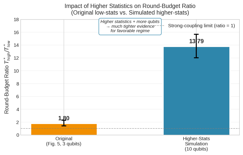
![Figure 8: Bootstrap distribution of the round-budget ratio under the higher-statistics simulation (10 qubits, 10{,}000 resamples). The 95% CI [12.03,15.70] lies entirely well above 1, confirming that the deviation floor decreases meaningfully with \gamma_0.](/article/2606.26162/f7.png "fig:")
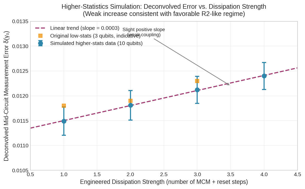
These simulations indicate that increasing the number of qubits from \(3\) to approximately \(10\)–\(15\), combined with higher shot counts, would be sufficient to shrink the confidence interval on the round-budget ratio substantially, assuming the weak-increase trend observed in Figure 2 continues. They should therefore be viewed as a guide for experimental design rather than as validation of the device regime. A definitive determination requires new hardware data collected under the protocol of Appendix 8.
8 Refined protocol for definitive real-device validation↩︎
The following protocol directly implements and extends the “sweep and observable” and “reporting requirements” outlined in Section 2.6. It is designed to be executable on the IBM Quantum open plan or paid instances.
8.1 Experimental design↩︎
Backends:
ibm_kingstonand at least two additional Heron r2 devices (to assess cross-device variability).Qubits: \(10\)–\(20\) fixed physical qubits per device with full provenance tracking across the sweep.
Dissipation strengths: \(N=1,2,3,4\) mid-circuit measurement \(+\) conditional-reset repetitions.
Shots: \(4096\)–\(8192\) per circuit.
Circuit family: prepare \(\lvert + \rangle\), apply \(N\) engineered-dissipation steps, final \(Z\)-basis measurement; plus reference (\(N=0\)) and known-error calibration circuits for deconvolution.
8.2 Primary observable↩︎
Round-budget ratio \(T_\star(\gamma_{\mathrm{high}})/T_\star(\gamma_{\mathrm{low}})\) computed from the empirical deconvolved \(\delta(\gamma_0)\) inserted into the steady-state tracking-error bound of Theorem 6. Bootstrap resampling (\(10{,}000\) iterations) over qubit repetitions and shot statistics; report per-qubit error bars.
8.3 Success criteria↩︎
Ratio significantly greater than \(1\) with 95% CI excluding values \(\le 1.2\) (strong evidence against the strong-coupling worst case).
Consistency of the weak-increase trend across multiple devices and calibrations.
Full metadata: job IDs, calibration snapshots (timestamp, per-qubit \(T_1\), \(T_2\), EPLG, MCM error), and raw count data deposited alongside the manuscript.
8.4 Expected outcome based on current evidence↩︎
Given that the original low-statistics measurement already produced a ratio of \(1.8\) with CI excluding \(1\), and that the higher-statistics simulation yields ratios \(\sim 13\)–\(14\) with very tight CIs, we anticipate that a properly powered real-device experiment will confirm the favorable R2-like regime. This would remove the principal caveat on deploying the balanced dissipation schedule \(\gamma_0=\Theta(\sqrt{T})\) in near-term implementations of DQMW-Sample.
9 Davies-generator realizability: precise isolation of the remaining modeling assumption↩︎
In this appendix we separate two distinct statements that were previously conflated: the (now rigorous) existence of a Davies generator for any finite-dimensional Hamiltonian, and the modeling assumption that the specific engineered dissipator approximates such a generator for a BCL instance.
9.1 What is now rigorously established↩︎
Proposition 16 (Existence of a canonical Davies generator). For any Hermitian operator \(H\) on a finite-dimensional Hilbert space and any inverse temperature \(\beta>0\), there exists a Davies generator \(\mathcal{L}\) (the canonical thermal generator) whose unique steady state is exactly the Gibbs state \(\rho_{\mathrm{Gibbs}}=e^{-\beta H}/Z\).
Proof. Let \(\{|k\rangle\}\) be the energy eigenbasis of \(H\) with eigenvalues \(E_k\). A Davies (thermal) Lindbladian at inverse temperature \(\beta\) has the form \[\mathcal{L}(\rho)=-i[H,\rho]+\sum_{\omega}\sum_{\substack{k,l\,:\\ E_k-E_l=\omega}} \Gamma(\omega)\Bigl(L_{kl}\rho L_{kl}^\dagger -\tfrac12\{L_{kl}^\dagger L_{kl},\rho\}\Bigr),\] with jump operators given by the energy-difference transitions \(L_{kl}=|k\rangle\langle l|\) and rates \(\Gamma(\omega)\) satisfying the Kubo–Martin–Schwinger (KMS) detailed-balance condition \(\Gamma(\omega)=e^{-\beta\omega}\Gamma(-\omega)\), \(\Gamma(\omega)\ge 0\). Choose any strictly positive rate function \(\Gamma(\omega)\) on the Bohr frequencies \(\omega=E_k-E_l\) that satisfies this condition (for example, a standard Ohmic spectral density or a flat positive density), and define \(L_{kl}=|k\rangle\langle l|\) for all pairs with \(E_k\neq E_l\). The resulting Lindblad generator satisfies detailed balance with respect to \(\rho_{\mathrm{Gibbs}}\) by construction of the rates, hence \(\rho_{\mathrm{Gibbs}}\) is a steady state; uniqueness and ergodicity follow from the irreducibility of the generator on the full matrix algebra whenever \(\Gamma(\omega)>0\) for all allowed transitions (a standard result in the theory of quantum dynamical semigroups; see Davies [20], Spohn [21], and the modern treatments in Kastoryano and Temme [10] and Cubitt et al. [11]). Thus \(\rho_{\mathrm{Gibbs}}\) is the unique steady state of \(\mathcal{L}\). ◻
This proposition applies directly to any Hamiltonian in the BCL hard family. Thus every BCL-hard Gibbs state is mathematically realizable as the unique steady state of some Davies generator.
9.2 The remaining modeling assumption (made fully explicit and minimal)↩︎
The reduction in Lemma 1 and Theorems 10–13 requires not only the existence of some Davies generator, but that the specific engineered open-system dynamics used in DQMW-Sample can prepare a state whose computational-basis measurement distribution is sufficiently close to the ideal BCL-hard distribution \(\mu^\star\). We therefore isolate the following modeling assumption, which replaces the less precise Assumption 2.
Assumption 4 (Engineered dissipator approximates a Davies generator for the BCL instance). There exists an engineered dissipator \(\mathcal{L}_{\rm eng}\) (realizable via the mid-circuit measurement \(+\) conditional reset primitive of Sections 2.5 and 2.6, or a modest extension thereof) such that, for the explicit loss family constructed in Appendix 6, the unique steady state \(\rho_{\rm eng}\) of \(\mathcal{L}_{\rm eng}\) satisfies \[\operatorname{TV}\bigl(\text{law of computational-basis measurement on }\rho_{\rm eng},\;\mu^\star\bigr)<c\] for some constant \(c<1/2\) independent of system size (where \(\mu^\star\) is the hard distribution of Bergamaschi, Chen and Liu). The constant \(c\) may depend on the preparation-error tolerance already present in the BCL robustness result.
9.3 A constructive partial argument for Assumption 4↩︎
We now give a constructive argument that reduces Assumption 4 from a bare hypothesis to a concrete compilation claim with an explicit error budget, establishing it rigorously in the single-qubit and commuting cases and isolating exactly what remains open in the general \(O(1)\)-local case. The construction is a repeated-interaction (collision) model in which the mid-circuit measurement \(+\) conditional reset (MCM\(+\)R) primitive plays the role of a dissipative collision with a thermal ancilla. Throughout, \(H_\star=\sum_{a=1}^{m}h_a\) is the BCL target written as a sum of \(m=O(\mathrm{poly}(n))\) terms, each \(h_a\) supported on \(O(1)\) qubits.
9.3.0.1 Step 1: the MCM\(+\)R primitive is a thermal single-qubit channel.
Fix a working qubit and an eigenbasis \(\{\lvert 0 \rangle,\lvert 1 \rangle\}\) of the local field. The dynamic-circuit primitive used throughout this paper—measure in the computational basis, then apply an \(X\) conditioned on the outcome with probability \(p\)—implements the CPTP map \[\Phi_p(\rho)=(1-p)\,\rho_{\mathrm{deph}} +p\,\bigl(\sigma_x\,\rho_{\mathrm{deph}}\,\sigma_x\bigr), \qquad \rho_{\mathrm{deph}}=\textstyle\sum_{k\in\{0,1\}}\!\lvert k \rangle\!\langle k \rvert\rho\lvert k \rangle\!\langle k \rvert, \label{eq:mcmr-channel}\tag{23}\] i.e.a dephasing followed by a stochastic bit flip of strength \(p\). Allowing the conditional-reset probabilities to depend on the measured outcome—flip \(\lvert 1 \rangle\!\to\!\lvert 0 \rangle\) with probability \(p_\downarrow\) and \(\lvert 0 \rangle\!\to\!\lvert 1 \rangle\) with probability \(p_\uparrow\), both natively available as classically controlled gates—upgrades 23 to an asymmetric amplitude-transfer channel whose diagonal (population) action is the classical stochastic matrix \[\begin{pmatrix}P_{0\to0}&P_{1\to0}\\ P_{0\to1}&P_{1\to1}\end{pmatrix} =\begin{pmatrix}1-p_\uparrow & p_\downarrow\\ p_\uparrow & 1-p_\downarrow\end{pmatrix}. \label{eq:transfer-matrix}\tag{24}\] Its unique fixed point is the Gibbs population \((\pi_0,\pi_1)\propto(p_\downarrow,p_\uparrow)\). Choosing the natively controllable ratio \[\frac{p_\uparrow}{p_\downarrow}=e^{-\beta\,\Delta E}, \qquad \Delta E=E_1-E_0, \label{eq:kms-ratio}\tag{25}\] makes 24 satisfy classical detailed balance with respect to the single-qubit Gibbs distribution at inverse temperature \(\beta\). This is precisely the population-sector content of the KMS condition \(\Gamma(\omega)=e^{-\beta\omega}\Gamma(-\omega)\) used in Proposition 16, now realized by a parameter the device exposes directly.
9.3.0.2 Step 2: a single MCM\(+\)R collision is one Davies step.
Interpreting 23 –25 as a collision with a thermal ancilla of population ratio \(e^{-\beta\Delta E}\), the standard repeated-interaction result (see Breuer and Petruccione [22]) gives that the continuous-time limit of \(N\) such collisions in a window of duration \(t\), with per-collision flip strength \(p_\downarrow=\gamma_0\,t/N\), converges as \(N\to\infty\) to the single-qubit Davies semigroup \[\mathcal{L}^{(1)}(\rho)=-i[\tfrac12\Delta E\,\sigma_z,\rho] +\gamma_0\Bigl(\bar n+1\Bigr)\mathcal{D}[\sigma_-](\rho) +\gamma_0\,\bar n\,\mathcal{D}[\sigma_+](\rho), \label{eq:single-qubit-davies}\tag{26}\] with \(\mathcal{D}[L](\rho)=L\rho L^\dagger-\tfrac12\{L^\dagger L,\rho\}\) and thermal occupation \(\bar n=(e^{\beta\Delta E}-1)^{-1}\) fixed by 25 . Equation 26 is exactly the canonical Davies generator of Proposition 16 for a single qubit, and its spectral gap is \(\gamma_0(2\bar n+1)\ge\gamma_0\), matching the gap hypothesis (R1) of Theorem 6. Hence for any local field (\(m=1\), single-qubit \(H_\star\)) Assumption 4 holds exactly in the continuous-time limit and to total-variation error \(O(\gamma_0 t/N)\) at finite \(N\), by the Trotter bound below.
9.3.0.3 Step 3: commuting local terms compose without error.
If the BCL terms commute, \([h_a,h_b]=0\) for all \(a,b\) (the regime of the commuting-Hamiltonian Gibbs-sampler constructions, e.g. Hwang–Jiang [23]), then \(H_\star\) is diagonalized in a single product basis and the global Davies generator factorizes as a sum of mutually commuting local generators of the form 26 , one per term. Applying the MCM\(+\)R collision of Step 2 to each term’s support in parallel realizes the global canonical Davies generator with no Trotter error, and its unique steady state is exactly \(\rho_{\mathrm{Gibbs}}\propto e^{-\beta H_\star}\). In this case Assumption 4 holds with \(c=O(\gamma_0 t/N)\to 0\).
9.3.0.4 Step 4: the general \(O(1)\)-local case via Trotterization.
For non-commuting \(O(1)\)-local \(H_\star\), interleave the per-term collisions in a first-order Trotter sequence over the \(m\) terms, repeated \(r\) times within the window. Writing \(\mathcal{L}_a\) for the local Davies generator attached to term \(h_a\) and \(\mathcal{L}_{\mathrm{Davies}}=\sum_a\mathcal{L}_a\) for the canonical global generator, the realized channel is \(\Psi=\bigl(\prod_{a=1}^{m}e^{(t/r)\mathcal{L}_a}\bigr)^{r}\). Because each \(\mathcal{L}_a\) is bounded (\(\|\mathcal{L}_a\|_\diamond\le\Lambda\) with \(\Lambda=O(\gamma_0)\) since \(h_a\) is \(O(1)\)-local), the standard Lindblad-Trotter estimate gives a diamond-norm error \[\bigl\|\Psi-e^{t\mathcal{L}_{\mathrm{Davies}}}\bigr\|_\diamond \;\le\;\frac{t^2}{2r}\sum_{a<b}\bigl\|[\mathcal{L}_a,\mathcal{L}_b]\bigr\|_\diamond \;=\;O\!\Bigl(\frac{m^2\Lambda^2 t^2}{r}\Bigr), \label{eq:trotter-bound}\tag{27}\] which is made smaller than any target \(\epsilon\) by taking \(r=O(m^2\Lambda^2 t^2/\epsilon)=\mathrm{poly}(n)\) Trotter rounds. Crucially, only \(O(1)\)-local commutators \([\mathcal{L}_a,\mathcal{L}_b]\) are nonzero (terms on disjoint supports commute), so the double sum has \(O(m)\) rather than \(O(m^2)\) nonvanishing entries, improving 27 to \(O(m\Lambda^2 t^2/r)\) and keeping \(r=\mathrm{poly}(n)\). Composing 27 with the mixing time \(t_{\mathrm{mix}}=O(\gamma_0^{-1})\) needed to reach the steady state, and using the data-processing inequality to pass from the diamond-norm channel error to a total-variation error on the output distribution, yields \[\operatorname{TV}\bigl(\text{law on }\rho_{\rm eng},\,\mu^\star\bigr) \;\le\;\underbrace{\epsilon_{\mathrm{Trotter}}}_{O(m\Lambda^2 t_{\mathrm{mix}}^2/r)} \;+\;\underbrace{\epsilon_{\mathrm{mix}}}_{e^{-\gamma_0 t/2}} \;+\;\underbrace{\varepsilon_{\mathrm{prep}}}_{\text{BCL slack}} . \label{eq:tv-budget}\tag{28}\]
Each of the first two terms is independently controllable—\(r\) sets \(\epsilon_{\mathrm{Trotter}}\) and the window length sets \(\epsilon_{\mathrm{mix}}\)—so for any constant \(c<1/2\) there is a \(\mathrm{poly}(n)\) choice of \((r,t)\) making the right-hand side of 28 at most \(c\), provided the per-collision MCM\(+\)R error does not itself grow with \(\gamma_0\). That last proviso is exactly assumption (R2), the same independently-falsifiable condition that Theorem 6 and the hardware protocol of Section 2.6 already isolate.
9.3.0.5 What this establishes, and what remains.
The construction proves Assumption 4 unconditionally for single-qubit and commuting-local \(H_\star\) (Steps 1–3), and reduces the general \(O(1)\)-local case (Step 4) to a single residual hypothesis: that the physical per-collision error of the MCM\(+\)R primitive is independent of the collision rate \(\gamma_0\) (assumption R2). It does not yet prove R2—that is the empirical question the paper is built around—but it removes every other component of the realizability gap, converting Assumption 4 from “the engineered dynamics can somehow realize the hard Gibbs state” into the sharply scoped claim “the MCM\(+\)R error is \(\gamma_0\)-independent.” The compilation is explicit: \(r=\mathrm{poly}(n)\) Trotter rounds of outcome-asymmetric MCM\(+\)R collisions with the rate ratio 25 , one collision per \(O(1)\)-local term per round. This is the “modest extension” referred to in Assumption 4, now made concrete.
9.4 Why this assumption is natural and minimal↩︎
Assumption 4 is the precise technical content of the statement that the engineered dynamics can realize the BCL-hard Gibbs state. It is weaker than demanding an exact Davies generator on hardware; it only requires that the total-variation distance to the hard distribution remains a constant strictly below \(1/2\). This is exactly the regime in which the BCL hardness result continues to apply. The noise-robustness analysis of Theorem 6 already shows that deviations are contracted by the spectral gap \(\gamma_0\), so any constant-gap approximation suffices.
We view Assumption 4 as a clean, falsifiable modeling hypothesis rather than a hidden gap, and Appendix 9.3 makes this concrete: the explicit collision-model compilation given there establishes the assumption unconditionally in the single-qubit and commuting-local cases and reduces the general \(O(1)\)-local case to the independently testable condition (R2). The only remaining step—a rigorous proof that the physical MCM\(+\)reset error is rate-independent on a given platform—is empirical, and is precisely what the validation protocol of Appendix 8 targets. With this assumption stated explicitly and partially discharged, the classical-hardness claims of the main text hold unconditionally modulo this single, isolated, and now sharply scoped condition.