Determining the Structure of Dynamic Factor Models
January 01, 1970
Abstract
We propose two procedures for determining the number of dynamic factors, extending [1] and [2] to dynamic factor models where lagged factors may directly influence the observed variables. As an intermediate step, we develop a simple and computationally efficient alternating least squares algorithm that directly estimates the dynamic factors, rather than their static representations. By working with these direct estimates, our approach enables joint determination of the number of factors and the filter length. Our test is shown to be consistent under weaker conditions than those in [3] and [4]. We apply our procedures to estimate the number of primitive shocks in a large panel of US macroeconomic time series.
JEL classification: C10, C38, C51, C55
Key words and phrases: Dynamic Factor Model, Number of Factors, Filter Length, Alternating Least Squares
1 Introduction↩︎
Factor models are a central tool in empirical macroeconomics and finance for summarizing co-movements in large-dimensional time series. Their appeal lies in the idea that a small number of latent factors can explain the dynamics of many observed variables.
A fundamental distinction is between static and dynamic factor models. In a static factor model, the observables \(x_t\) depend only contemporaneously on a low-dimensional vector of factors \(f_t\), e.g., \(x_t = \lambda f_t + \varepsilon_t\), whereas a dynamic factor model allows lags of the factors to affect the observables, e.g., \(x_t = \sum_{k=0}^{m-1} \lambda_k f_{t-k} + \varepsilon_t\). The dynamic specification is more general and economically informative, as it captures delayed responses and propagation mechanisms that are central to macroeconomic and financial dynamics.2
While a large body of work has developed methods for estimating the number of static factors—see, for example, [1], [6], and [2]—the literature on estimating the number of dynamic factors remains relatively limited. Notable exceptions are [3] and [4]. These papers approach the problem by constructing a static representation of the dynamic factor model. Under the assumption that the static representations of the dynamic factors follow a VAR process with a lower-dimensional innovation, [3] and [4] develop consistent procedures for estimating the number of dynamic factors. Although VAR models provide a flexible and widely used framework for capturing time series dynamics, the literature on the study of the static factor models shows that a VAR specification for the static factors is not necessary for either estimating the factors or determining their number. This raises the question of whether it is possible to consistently estimate the number of dynamic factors without imposing a VAR model on the factors.
This paper proposes a new approach to estimating the number of dynamic factors that does not rely on the assumption that the factors follow a VAR process. Instead, our method requires that the second moment matrix of the static representations of the dynamic factors be positive definite, a substantially weaker condition than imposing a parametric VAR structure. Our approach is enabled by directly estimating the dynamic factors using an alternating least squares algorithm. The procedure iteratively updates factors and loadings via simple least squares steps, making it computationally efficient and scalable to large datasets. When applied to static factor models, the alternating least squares estimator reduces to the principal components estimator commonly used in static factor models. We establish consistency under double asymptotics when both the number of samples and the dimension of the observed variable diverge, obtaining the standard convergence rates typically associated with the estimation of static factors. By leveraging consistent estimators of the dynamic factors, we propose two procedures that jointly estimate the number of dynamic factors and the filter length, defined as the length of the horizon over which current and lagged factors exert a direct effect on the observed variables.
Our approach extends the criteria of [2] and [1] to dynamic factor models. Under general Assumptions to be introduced in Sections 2 and 4, the number of dynamic factors and the filter length of the dynamic factor model are jointly identified asymptotically independently of any parametric specification for the stochastic process governing the dynamic factors. In particular, if the dynamic factors follow a VAR\((p)\) process, the identification of the filter length is invariant to the choice of the lag order \(p\). We show in Section 4.3 that when the dynamic factors follow a VAR process, the lag order selection can be done using the standard BIC criterion with the unobserved factors replaced with their estimates.
The eigenvalue ratio test of [2] identifies the number of factors by detecting the point at which the ratio of consecutive singular values of the data matrix diverges. We extend this idea to dynamic factor models by introducing a notion of ‘dynamic’ singular values, defined as the spectral norm of the residual matrix after removing a given number of estimated dynamic factors. Building on this concept, we propose the dynamic singular value ratio test, which generalizes the eigenvalue ratio test of [2] and coincides with it when applied to a static factor model. Moreover, the proposed framework can be used to determine the filter length of the dynamic factor model by examining the behavior of ratios of consecutive dynamic singular values as the filter length varies for a fixed number of dynamic factors.
The information criterion of [1] selects the number of static factors by augmenting the residual variance with a penalty term that increases with the number of static factors. Our second procedure extends this approach to dynamic factor models by employing a penalty term that depends on both the number of dynamic factors and the filter length. When we restrict the filter length to one, the proposed criterion reduces to that of [1], up to a constant factor of two in the penalty term.
1.1 Related literature and contributions of this paper↩︎
There is a large literature on dynamic factor models, which can be broadly divided into two classes. The first class comprises generalized dynamic factor models with infinite filter length, which do not admit a finite-dimensional static representation. The second class consists of models with a finite filter length, for which a static representation exists. Our work falls into the second category: the dynamic factor models with a finite filter length. What distinguishes our work from many existing ones is that we work directly with the dynamic factors themselves, rather than the static representations.
The generalized dynamic factor model with infinite filter length was introduced by [5], who proposed estimation based on frequency-domain principal components. Subsequent work has developed one-sided representations, estimation methods, and asymptotic theory for these models: [7], [8], and [9]. Tests for the number of dynamic factors in the generalized dynamic factor framework have also been proposed by [10] and [6]. However, the greater generality afforded by infinite-length filters typically requires the dynamic factors to be serially uncorrelated processes for identification. We focus our attention on dynamic factor models with finite length filter in this paper.
A separate strand of the literature studies the static representations of dynamic factor models. [11] and [12] provide inferential theory for static factors estimated by principal components and quasi–maximum likelihood, respectively. Procedures for determining the number of static factors include information criteria [1] and eigenvalue-ratio tests [2], among others. Despite this extensive literature, comparatively little attention has been paid to the direct estimation of dynamic factors. An exception is [13], who studies Bayesian estimation of dynamic factor models. This paper is most closely related to [3] and [4], who study the estimation of the number of dynamic factors in models with finite filter length.
To summarize, our contributions are as follows.
First, we generalize the procedures of [1] and [2] to estimate the number of dynamic factors in dynamic factor models. Our approach is more robust than those of [3] and [4], as it does not require imposing a VAR structure on the static factors.
Second, our procedure provides a consistent estimator of the filter length, jointly with the number of dynamic factors, which, to the best of our knowledge, is the first in the literature. Identifying the extent to which primitive shocks directly affect the economy is of independent interest. For instance, using the FRED–MD dataset of [14] over the sample period March 1973 to July 2025, the filter length is estimated to be two.3
Third, we examine the finite-sample performance of our testing procedure and show that they outperform those of [3] and [4] across a range of designs in determining \(q\).
Finally, we establish the consistency of the proposed alternating least squares estimator in estimating the dynamic factors. Furthermore, when the dynamic factors follow a VAR\((p)\) process, we show that the lag order selection can be done using the standard BIC criterion with the unobserved factors replaced with their estimates.
We denote by \(\|\cdot\|\) the Euclidean norm when applied to vectors and the associated spectral (operator) norm when applied to matrices. The Frobenius norm is denoted by \({\left\vert\kern-0.3ex\left\vert\kern-0.3ex\left\vert \cdot \right\vert\kern-0.3ex\right\vert\kern-0.3ex\right\vert}\). The row-major vectorization operator is denoted by \(\mathop{\mathrm{vec}}(\cdot)\). For a symmetric matrix \(A\), the notation \(A>0\) and \(A\geq0\) indicates that \(A\) is positive definite and positive semi-definite, respectively. We denote \(P_A=A(A'A)^{-1}A'\) and \(M_A=I-P_A\) for any matrices \(A\). We write \(\lceil x \rceil\) for the smallest integer greater than or equal to \(x\) and \(\lfloor x\rfloor\) for the largest integer greater than or equal to \(x\). Throughout, \(q\) denotes the number of dynamic factors, \(m\) the filter length, and \(r = qm\) the corresponding number of static factors. Finally, we denote \(\mathbb{Z}\) and \(\mathbb{R}\) the set of nonnegative integers and real numbers, respectively.
The remainder of the paper is organized as follows. Section 2 presents the model and discusses representations of the dynamic factors. Section 3 describes the alternating least squares estimation procedure and the consistency of the proposed method. Section 4 develops two methods for determining the number of dynamic factors and the filter length. Section 5 reports simulation evidence on the finite-sample performance of the proposed procedures. Section 6 provides an empirical application. Section 7 concludes. All technical proofs are collected in the Appendix.
2 Model, Assumptions, and Representations↩︎
2.1 Model↩︎
We consider the dynamic factor model \[x_{it} = \sum_{k=0}^{m-1} \lambda_{ik}' f_{t-k} + \varepsilon_{it}, \qquad i=1,\ldots,N,\; t=1,\ldots,T,\] where \(f_t \in \mathbb{R}^q\) are the dynamic factors and \(\lambda_{ik} \in \mathbb{R}^q\) are factor loadings. When \(m=1\), the model reduces to a static factor model. When \(m=\infty\), it corresponds to the generalized dynamic factor model of [5]. However, we restrict attention to the finite-filter case \(m<\infty\), which can be viewed either as a finite-dimensional specialization of [5] or as a dynamic generalization of the conventional static factor model of [11] and [15]. The model admits a static representation, \[x_{it} = \gamma_i' g_t + \varepsilon_{it}, \qquad g_t = \begin{pmatrix} f_{t} \\ \vdots \\ f_{t-m+1} \end{pmatrix}, \qquad \gamma_i = \begin{pmatrix} \lambda_{i,0} \\ \vdots \\ \lambda_{i,m-1} \end{pmatrix},\] where \(g_t \in \mathbb{R}^{qm}\) is the static factors constructed using the current and lags of the dynamic factors. Define \[x_t = (x_{1t},\ldots,x_{Nt})', \qquad \varepsilon_t = (\varepsilon_{1t},\ldots,\varepsilon_{Nt})',\] and stack observations over time as \[X = (x_1,\ldots,x_T)', \qquad E = (\varepsilon_1,\ldots,\varepsilon_T)', \qquad G = (g_1,\ldots,g_T)'.\] The model can then be written compactly as \[x_t = \Gamma g_t + \varepsilon_t, \qquad X = G \Gamma' + E,\] where \(\Gamma = (\lambda_{0},\ldots,\lambda_{m-1})\) is the \(N \times qm\) matrix of factor loadings. Let \(F_{-k} = (f_{1-k},\ldots,f_{T-k})'\) collect the \(k\)-th lag of the factors so that \(G = \big( F_{0}, \ldots, F_{-m+1} \big)\). Then, we may write the model in its dynamic form \[X = \sum_{k=0}^{m-1} F_{-k} \lambda_k' + E.\] We let \(F = F_0\) for the \(T \times q\) matrix collecting \((f_t)_{t=1}^T\).
The dynamic factor model can be regarded as a static factor model with the restrictions that \(m\) blocks of the static factors are given as leads and lags of themselves. Thus, direct estimation of dynamic factors is always more parsimonious than estimation based on static representations.
2.2 Assumptions↩︎
We impose the following two assumptions, which are required to establish the consistency of the estimated factors and factor loadings. We’ll introduce two additional assumptions in Section 4, which are needed to establish consistency for tests of the number of dynamic factors and filter length.
Assumption 1. The factors and factor loadings satisfy \[\frac{1}{T} G'G \to_p M_g > 0, \quad \frac{1}{N} \Gamma' \Gamma \to_p M_\gamma > 0\] as \(T \to \infty\) and \(N \to \infty\), where \(M_g\) and \(M_\gamma\) are \(qm \times qm\) positive definite matrices.
Assumption 2. The idiosyncratic errors satisfy \[\|E\| = O_p(\sqrt{\max(N,T)}).\]
Assumption 1 requires that the static representations \(g_t\) of the dynamic factors \(f_t\) are strong factors. Assumption 1 holds whenever the dynamic factors \((f_t)\) are stationary with a spectral density matrix that is positive definite on a set of frequencies with positive measure, which includes any stationary and invertible VARMA processes with non-degenerate innovation as a special case. In fact, non-degenerate VAR processes have strictly positive definite spectral density matrix for all frequencies, so that Assumption 1 is a strictly weaker condition.4 Note that both [3] and [4] also impose Assumption 1 so that the number of static factors \(r\) can be consistently estimated. In contrast, imposing a simple VMA(\(1\)) model for \((f_t)\) will invalidate both [3] and [4] because a VMA(\(1\)) model cannot be written as finite lag VAR model.5
Assumption 2 is standard in the factor models literature and used to limit the amount of cross-sectional and serial correlations in the errors, e.g., [6], [2], [16], and [17].
2.3 Dynamic Representations↩︎
Let \((q_0, m_0)\) denote the unknown true structure, i.e., the number of dynamic factors and filter length, of the dynamic factor model, and let \((q, m)\) be a general notation used to denote the number of dynamic factors and the filter length. It is well known that the dynamic factor model with structure \((q_0,m_0)\) has an observationally equivalent static representation with \((q,m)=(q_0m_0,1)\). Dynamic factor model may also admit multiple dynamic representations other than the fully static representation. In other words, there may exist multiple dynamic factor models with different structures \((q, m)\) whose common components are observationally equivalent.
For example, consider a model with \((q,m)=(2,3)\) given by \[x_t = \sum_{k=0}^{2} \lambda_k f_{t-k} + \varepsilon_t, \quad f_t \in \mathbb{R}^2.\] It is well known that this model has a static representation given as \[\begin{align} \label{example2} x_t &= \begin{pmatrix} \lambda_1 & \lambda_2 & \lambda_3 \end{pmatrix}g_{t} + \varepsilon_t, \end{align}\tag{1}\] and \(g_{t} = \begin{pmatrix} f_{t} \\ f_{t-1} \\ f_{t-2} \end{pmatrix}\in\mathbb{R}^6\). This model can also equivalently be written as \[\begin{align} \label{example1} x_t &= \begin{pmatrix} \lambda_{1,1} & \lambda_{1,2} & \lambda_{2,2}-\lambda_{3,1} \end{pmatrix} g_{t} + \begin{pmatrix} \lambda_{2,1}-\lambda_{1,2} & \lambda_{3,1} & \lambda_{3,2} \end{pmatrix} g_{t-1} + \varepsilon_t \end{align}\tag{2}\] where \(g_{t} = \begin{pmatrix} f_{t,1} \\ f_{t,2} + f_{t-1,1} \\ f_{t-1,2} \end{pmatrix}\in\mathbb{R}^3\). Here, \(f_{t-k,j}\) and \(\lambda_{k,j}\) denote the \(j\)-th element of \(f_{t-k}\) and the \(j\)-th column of \(\lambda_k\), respectively. The model 1 with the structure \((q,m) = (6,1)\) and the model 2 with the structure \((q,m) = (3,2)\) are observationally equivalent to the original model with structure \((q,m)=(2,3)\).
Since there may be multiple pairs \((q,m)\) with the correct specification, we denote the pair \((q,m)\) with the smallest \(q\) as the true structure \((q_0, m_0)\). If \(m < m_0\), more factors are needed to achieve correct specification, and if \(q>q_0\), a smaller filter length may suffice to preserve correct specification. The following proposition shows that such representations are always possible and gives the minimal number of additional factors required, given \(m<m_0\), and the smallest \(m\) attainable when \(q>q_0\).
Let \((q_0, m_0)\) denote the true number of dynamic factors and the filter length in the model \[x_t = \sum_{k=0}^{m_0-1}\lambda_kf_{t-k},\quad f_t\in \mathbb{R}^{q_0}\] for the common component with \(q_0\geq1\) and \(m_0\geq1\). Then, the common component admits alternative dynamic factor representations of the form \[x_t = \sum_{k=0}^{m-1}\Gamma_kg_{t-k},\quad g_t \in\mathbb{R}^q\] with the following properties:
Shorter filters require more factors, i.e., \[\left\{(q,m):q\geq \left\lceil \frac{q_0 m_0}{m} \right\rceil, \quad 1 \le m < m_0\right\}.\]
More factors allow shorter filters, i.e., \[\left\{(q,m):q>q_0,\quad m\geq\left\lceil \frac{q_0 m_0}{q} \right\rceil\right\}.\]
Moreover, given Assumption 1, the lower bound for \(q\) and \(m\), i.e., \(\left\lceil \frac{q_0 m_0}{m} \right\rceil\) and \(\left\lceil \frac{q_0 m_0}{q} \right\rceil\), are sharp in that representations with the structures given by \[(q, m) = \left( \left\lceil \frac{q_0 m_0}{m} \right\rceil-1, \, m \right), \quad 1 \le m < m_0,\] or \[(q, m) = \left( q, \, \left\lceil \frac{q_0 m_0}{q} \right\rceil-1 \right), \quad q > q_0,\] does not lead to an observationally equivalent model.
Let \(q_0\geq0,\) \(m_0\geq0\) be given, and consider disjoint partition of \(\mathbb{Z}^2\) given by \[\begin{align}\label{partition95set} S_1&=\left\{(q,m)\in \mathbb{Z}^2 : q_0\le q,\;\left\lceil \frac{q_0 m_0}{q} \right\rceil \le m \right\}\\ S_2&=\left\{(q,m)\in \mathbb{Z}^2 : m=0 \right\} \cup \left\{(q,m)\in \mathbb{Z}^2 : 1\le m<m_0,\;q<\left\lceil \frac{q_0 m_0}{m} \right\rceil \right\},\\ S_3&=\left\{(q,m)\in \mathbb{Z}^2 : m\ge m_0,\;q<q_0 \right\}, \end{align}\tag{3}\] where under \(q_0=0\) or \(m_0=0\) we let \(S_1=\mathbb{Z}^2\) and \(S_2=S_3=\emptyset\). Proposition [alt95spec] implies that \(S_1\) is the set of structures \((q,m)\) that yield models observationally equivalent to the true model with \((q_0,m_0)\). Furthermore, structures in \(S_2\) lead to mis-specification. We introduce Assumption 4 in Section 4 so that structures in \(S_3\) also lead to mis-specification as long as \(m\) is finite.
3 Estimation↩︎
In the dynamic factor model, \[x_t = \sum_{k=0}^{m-1} \lambda_k f_{t-k} + \varepsilon_t, \quad t=1,\ldots,T,\] the dynamic factors \((f_t)\) are indexed from \(t = 2-m\) to \(t = T\) to account for the lagged factors entering the measurement equation. We jointly estimate \((f_t)_{t=2-m}^{T}\) and \((\lambda_k)_{k=0}^{m-1}\) by minimizing the least squares objective \[\begin{align} \label{obj95fn} \frac{1}{NT} {\left\vert\kern-0.3ex\left\vert\kern-0.3ex\left\vert X - \sum_{k=0}^{m-1} F_{-k} \lambda_k' \right\vert\kern-0.3ex\right\vert\kern-0.3ex\right\vert}^2 = \frac{1}{NT}\sum_{t=1}^T\left\|x_t-\sum_{k=0}^{m-1} \lambda_k f_{t-k}\right\|^2 \end{align}\tag{4}\] over \((f_t)\) and \((\lambda_k)\). The first-order conditions for the factor loadings \((\lambda_j)\) are \[\begin{align} \label{foc95lambda} \sum_{k=0}^{m-1} \hat{\lambda}_k \hat{F}_{-k}' \hat{F}_{-j} = X' \hat{F}_{-j}, \quad j=0,\ldots,m-1. \end{align}\tag{5}\] The first-order conditions for \((f_t)\) are \[\begin{align} \label{foc95f} \sum_{j=\max(0,1-t)}^{\min(m-1,T-t)}\lambda_j'\left(x_{t+j}-\sum_{k=0}^{m-1}\lambda_kf_{t+j-k}\right) = 0 \end{align}\tag{6}\] for \(t=2-m,\ldots,T\).
We minimize 4 using an alternating least squares procedure. We start with an initial guess for \((\hat{\lambda}_k)\). Given \((\hat{\lambda}_k)\), we may update \((f_t)\) by solving 6 . Given \((\hat{f}_t)\), we may update \((\lambda_k)\) by solving 5 . We repeat the updating steps until convergence. The first-order conditions 5 defines a multivariate regression with rank \(qm\), which has a closed-form solution. The first-order condition 6 can be efficiently solved using the discrete Fourier transform, requiring inversion of only \(q \times q\) matrices.6 Since each step minimizes a least squares objective, the algorithm guarantees a monotone decrease of the objective function. The minimization problem is not convex, and the alternating least squares algorithm generally does not converge to the global minimum. We try multiple initial values and choose the solution that obtains the smallest objective function value in practice.
3.1 Consistency↩︎
Before introducing the test for the structure \((q,m)\) of the dynamic factor models, we first show that the estimated dynamic factors are consistent.
Let Assumptions 1 and 2 hold. Let \(S_1\) be as defined in 3 and \(\hat{G}\) be a minimizer of the squared error 4 with structure \((q,m)\in S_1\). We have \[\begin{align} \frac{1}{\sqrt{T}}{\left\vert\kern-0.3ex\left\vert\kern-0.3ex\left\vert M_{\hat{G}}G_0 \right\vert\kern-0.3ex\right\vert\kern-0.3ex\right\vert} = O_p\left(\frac{1}{\sqrt{N}}+\frac{1}{\sqrt{T}}\right). \end{align}\]
Proposition [consistency951] shows that the factors \(g_t\) estimated via the alternating least squares applied to the dynamic factors \(f_t\) are consistent as long as \((q,m)\in S_1\). Theorem 1 of [1] implies \(g_t\) estimated using the structure \((q,m)\) in the set \(\{(q,m):qm\geq q_0m_0,\:m=1\}\), i.e., the set of structures associated with the correct or over-specified static representations with \(m=1\), is consistent. Proposition [consistency951] extends this result to all the structures \((q,m)\in S_1\) that can lead to observationally equivalent common components by directly estimating models with \(m>1\). The alternating least squares estimator for \(f_t\) imposes a specific structure on \(g_t\), whereby its \(m\) blocks correspond to leads and lags of the same underlying dynamic factors. That is, \[\hat{g}_t = \begin{pmatrix} \hat{f}_t \\ \vdots \\ \hat{f}_{t-m+1} \end{pmatrix}.\] In contrast, when \(g_t\) is estimated directly via principal components, this temporal structure is not imposed, and the above relation need not hold. This distinction is crucial when determining the structural dimensions \((q_0, m_0)\) of the dynamic factor model.
4 Testing for Number of Dynamic Factors and Filter Length↩︎
4.1 Test Based on Dynamic Singular Value Ratio↩︎
To construct a test for the true model \((q_0,m_0)\), we employ a notion of dynamic singular values, which generalizes the classical singular value decomposition to incorporate temporal structure. Formally, let \(\delta_{q+1,m}(X)\) denote the \((q+1)\)-th dynamic singular value of a matrix \(X\) with filter length \(m\), defined as \[\delta_{q+1,m}(X) = \min_{(f_t) \in \mathbb{R}^{q}, \, (\lambda_k) \in \mathbb{R}^{q}} \Big\| X - \sum_{k=0}^{m-1} F_{-k} \lambda_k' \Big\|,\] where \(q \ge 0\) and \(m \ge 0\) with the convention that \(\delta_{1,m}(X)\) or \(\delta_{q+1,0}(X)\) denotes spectral norm of \(X\). Note that we let \((f_t)\) and \((\lambda_k)\) be optimization arguments, not the true factors and factor loadings, whenever they appear as arguments within a minimization problem. Dynamic singular value generalizes the notion of the standard singular values; When \(m=1\), \(\delta_{q+1,1}(X)\) coincides with the usual \((q+1)\)-th singular value of \(X\): \[\delta_{q+1,1}(X) = \min_{F \in \mathbb{R}^{T \times q}, \, \lambda \in \mathbb{R}^{N \times q}} \| X - F \lambda' \|.\] Note that \(\delta_{q+1,m}(X)\) can be interpreted as the minimization problem \[\begin{align} \delta_{qm+1,1}(X) = \min_{G\in\mathbb{R}^{T\times qm},\Gamma\in\mathbb{R}^{T\times qm}}\left\|X-G\Gamma'\right\| \end{align}\] with the additional constraints that \(m\) blocks of \(G\in\mathbb{R}^{T\times qm}\) with \(q\) columns are given as leads and lags of each other. This implies that we have \(\delta_{q_0m_0+1,1}(X)\leq \delta_{q_0+1,m_0}(X)\) for any \((q_0,m_0)\). More generally, we have \[\begin{align} \delta_{q+1,m}(X) \leq \delta_{q_0+1,m_0}(X) \end{align}\] for any integer \((q,m)\in S_1\) because \(\delta_{q+1,m}(X)\) minimizes the objective function over a larger space due to Proposition [alt95spec].
Assumption 3. For any \(\epsilon>0\), there exists a constant \(c_0>0\) such that \[\mathbb{P}\!\left( \frac{1}{\sqrt{N+T}} \, \delta_{k+1,1}(E) < c_0 \right) \le \epsilon\] for all \(k=0,\ldots,k_{\max}\) and for all sufficiently large \(N\) and \(T\), where \(k_{\max}\) is a fixed integer.
Assumption 4. For any \(\epsilon>0\), there exists a constant \(c_2>0\) such that \[\mathbb{P}\!\left( \frac{1}{\sqrt{NT}} \, \delta_{q+1,m}\!\left(\sum_{k=0}^{m_0-1} F_{-k}\lambda_k'\right) < c_2 \right) \le \epsilon\] for all \(q=0,\ldots,q_0-1\) and \(m=1,\ldots,m_{\max}\), and for all sufficiently large \(N\) and \(T\), where \(m_{max}\) is a fixed integer.
Assumption 3 requires that the leading singular values of \(\frac{1}{\sqrt{\max(N,T)}}E\) be bounded away from zero in probability. Under general conditions, the number of singular values that remain bounded away from zero can be shown to grow at the rate \(\min(N,T)\); see, for example, [2]. As a direct implication of Assumption 3, for any \(\epsilon>0\) there exists \(c_0>0\) such that \[\mathbb{P}\!\left( \frac{1}{\sqrt{N+T}} \, \delta_{q+1,m}(E) < c_0 \right) \le \epsilon\] for all pairs \((q,m)\) satisfying \(qm \le k_{\max}\), and for all sufficiently large \(N,T\).
Assumption 4 imposes a lower bound on the dynamic singular values of the common component. Note that \[\begin{align} \frac{1}{\sqrt{NT}} \delta_{q_0,m_0}\!\left(\sum_{k=0}^{m_0-1} F_{-k}\lambda_k'\right) &\ge \frac{1}{\sqrt{NT}} \delta_{(q_0-1)m_0+1,1}\!\left(\sum_{k=0}^{m_0-1} F_{-k}\lambda_k'\right) \\ &= \frac{1}{\sqrt{NT}} \delta_{q_0 m_0 - m_0 + 1,1}(G\Gamma'), \end{align}\] where the inequality follows from the additional restrictions imposed on the minimization problem on the left hand side. The term \(\frac{1}{\sqrt{NT}} \delta_{q_0 m_0 - m_0 + 1,1}(G\Gamma')\) is strictly positive in the limit provided that \(m_0\ge1\). Indeed, the \(k\)-th singular value of \((NT)^{-1/2}G\Gamma'\) equals the square root of the \(k\)-th eigenvalue of \[\left(\frac{1}{N}G'G\right)\left(\frac{1}{T}\Gamma'\Gamma\right),\] which is bounded away from zero for all \(k=1,\ldots,q_0m_0\) by Assumption 1. Consequently, \[\frac{1}{\sqrt{NT}} \delta_{q,m}\!\left(\sum_{k=0}^{m_0-1}F_{-k}\lambda_k'\right)\] is bounded away from zero in probability for all \(q=1,\ldots,q_0\) and \(m=1,\ldots,m_0\).
Assumption 4 further requires this lower bound to persist for \(m=m_0+1,\ldots,m_{\max}\). This restriction rules out the possibility that omitted dynamic factors can be fully recovered by increasing the filter length of the remaining factors. In other words, when fewer than \(q_0\) dynamic factors are extracted, enlarging the lag polynomial alone is insufficient to span the factor space associated with the omitted components.
This requirement is satisfied whenever the \(q_0\) largest eigenvalues of the spectral density matrix of the common component diverge at the rate \(N\) on a set of frequencies with positive measure, which is more lenient than the standard assumption of divergence almost everywhere (see, e.g., [5], [7], [8]). If \((f_t)\) is given by a stationary and invertible VARMA process with non-degenerate innovation, \(q_0\) largest eigenvalues diverge at the rate \(N\) for all frequencies so that Assumption 4 is satisfied.
Assumption 4 is imposed so that the structures in the set \(S_3\) defined in 3 are mis-specified as long as \(m\leq m_{max}\). This implies that given \(q_{max}\) and \(m_{max}\) satisfying \(q_0\leq q_{max}, m_0\leq m_{max}\), the set of correctly specified structures \((q,m)\) are given by \[\mathcal{C}=\left\{(q,m)\in \mathbb{Z}^2 : q_0\le q\leq q_{max},\;\left\lceil \frac{q_0 m_0}{q} \right\rceil \le m \leq m_{max}\right\}.\] We construct a test based on estimated dynamic singular values. Let \(\hat{\delta}_{q+1,m}(X)\) denote the estimated \((q+1)\)-th dynamic singular value, defined as the spectral norm of the residual matrix obtained after fitting a dynamic factor model with \(q\) factors and filter length \(m\). Specifically, \[\begin{align} \hat{\delta}_{q+1,m}(X) = \left\| X-\sum_{k=0}^{m-1}\hat{F}_{-k}^{(q)}\hat{\lambda}_k^{(q)\prime} \right\|, \end{align}\] where \((\hat{F}_{-k}^{(q)},\hat{\lambda}_k^{(q)})_{k=1}^m\) are the least-squares estimators obtained by minimizing the squared error under \(q\) dynamic factors with \(m\) filter length, i.e., the objective function 4 .
It is important to note that the alternating least squares algorithm yields the minimizer of the Frobenius norm, whereas the dynamic singular value is defined as the minimum of the spectral norm. The two minimization problems coincide in the static case (\(m=1\)), in which case \(\hat{\delta}_{q+1,1}(X)\) reduces to the usual \((q+1)\)-th singular value of \(X\). For \(m>1\), the two minimizers generally differ. While dynamic singular values can in principle be computed by directly minimizing the spectral norm, we rely on the Frobenius-norm solution for computational tractability. This approximation does not affect the asymptotic validity of the proposed test, as seen in Theorems 1 and 2.
As can be seen from the proofs of Theorems 1 and 2, we may characterize the asymptotic behavior of \(\hat{\delta}_{q+1,m}(X)\) under Assumptions 1, 2, and 4. In other words, we may show that there exists \(q_{max}\) and \(m_{max}\) such that for all \(0\leq q\leq q_{max}\) and \(0\leq m\leq m_{max}\), we have \[\begin{align} \hat{\delta}_{q+1,m}(X) = \begin{cases} O_p(\sqrt{NT}) & (q,m)\notin\mathcal{C}\\ O_p(\sqrt{N+T}) &(q,m)\in\mathcal{C} \end{cases}. \end{align}\] This behavior of the estimated dynamic singular values \(\hat{\delta}_{q+1,m}(X)\) motivates the dynamic singular value ratio tests given in Theorem 1 and 2 below.
In Theorem 1, we fix \(m\) and estimate the number of dynamic factors using a ratio-type statistic based on adjacent estimated dynamic singular values.
Theorem 1. Suppose Assumptions 1, 2, 3, and 4 hold with \(q_0\geq1\) and \(m_0\geq1\). Let \(k_{max}\) and \(m_{max}\) be integers given in Assumptions 3 and 4 and let \(q_{\max}\) be an integer satisfying \(q_0m_0+q_{max}m_{max}\leq k_{max}\). Fix \(m\ge1\) and define \[\begin{align} \hat{q} = \mathop{\rm argmax}\limits_{1\le q\le q_{\max}} \frac{\hat{\delta}_{q,m}(X)}{\hat{\delta}_{q+1,m}(X)}, \end{align}\] If \(m_0\le m\le m_{\max}\), then \[\begin{align} \mathbb{P}\{\hat{q}=q_0\}\to1 \quad\text{as } N,T\to\infty. \end{align}\] If instead \(m<m_0\), then \[\begin{align} \mathbb{P}\!\left\{\hat{q}=\left\lceil\frac{q_0m_0}{m}\right\rceil\right\}\to1, \end{align}\] where \(\lceil\cdot\rceil\) denotes the ceiling function.
Theorem 1 shows that, when the filter length is at least as large as \(m_0\), the ratio statistic consistently identifies the true number of dynamic factors. When the filter length smaller than \(m_0\), the procedure selects the minimal number of factors required to span the true common component, reflecting the observational equivalence between \((q_0,m_0)\) and alternative \((q,m)\) representations discussed in Proposition [alt95spec]. When \(m=1\), the test statistic coincides with the eigenvalue ratio (ER) test of [2] and consistently estimates the number of static factors, \(r=q_0m_0\). Theorem 1 thus generalizes the ER test to dynamic factor models by allowing the filter length \(m\) to exceed one.
In Theorem 2, we fix \(q\) and estimate the filter length using a similar ratio-type statistic.
Theorem 2. Suppose Assumptions 1, 2, 3, and 4 hold with \(q_0\geq1\) and \(m_0\geq1\). Let \(k_{max}\) and \(m_{max}\) be integers given in Assumptions 3 and 4 and let \(q_{\max}\) be an integer satisfying \(q_0m_0+q_{max}m_{max}\leq k_{max}\). Fix \(q\geq1\) and define \[\begin{align} \hat{m} = \mathop{\rm argmax}\limits_{1\le m\le m_{\max}} \frac{\hat{\delta}_{q+1,m-1}(X)}{\hat{\delta}_{q+1,m}(X)}, \end{align}\] where \(\hat{q}_{q+1,0}(X)\) denotes the spectral norm of \(X\). If \(q=q_0\ge1\), then \[\begin{align} \mathbb{P}\{\hat{m}=m_0\}\to1 \end{align}\] as \(N,T\to\infty\). If \(q>q_0\), then \[\begin{align} \mathbb{P}\!\left\{ \hat{m}=\left\lceil \frac{q_0m_0}{q}\right\rceil \right\} \to1, \end{align}\] where \(\lceil\cdot\rceil\) denotes the ceiling operator.
Theorem 2 provides a consistent estimator of the true filter length \(m\) in dynamic factor models. If \(q=q_0\), the test uncovers the true filter length. If \(q>q_0\), the test select the smallest filter length required to span the true common component. The case \(q<q_0\) is excluded. Under Assumption [lower95bound95common], \(\delta_{q+1,m}(X)=O_p(\sqrt{NT})\) for all \(m\le m_{\max}\) when \(q<q_0\). As a result, \(DR_{q,m}(X)\) may not diverge at \(m=m_0\), and ratio-based tests for the filter length fail when not enough dynamic factors are included.
To recover \((q_0,m_0)\) using Theorem 1 and 2, we may start with any \(m\) sufficiently large so that \(m\geq m_0\). Using \(m\geq m_0\), we may recover \(q_0\) using Theorem 1. Then, using Theorem 2, we may recover \(m_0\) using \(q=q_0\).
4.2 Test Based on Information Criteria↩︎
Let \(V(q,m)\) denote the mean squared errors when the structure \((q,m)\) is used to estimate a dynamic factor model, i.e., \[\begin{align} V(q,m) = \frac{1}{NT} {\left\vert\kern-0.3ex\left\vert\kern-0.3ex\left\vert X - \sum_{k=0}^{m-1} \hat{F}_{-k}^{(q)} \hat{\lambda}_k^{(q)\prime} \right\vert\kern-0.3ex\right\vert\kern-0.3ex\right\vert}^2, \end{align}\] where \((\hat{F}_{-k}^{(q)},\hat{\lambda}_k^{(q)})_{k=0}^{m-1}\) is the least squares estimator obtained under the structure \((q,m)\).
Following [1], we augment the residual variance with a penalty term. The key is to construct a penalty sequence that vanishes asymptotically, yet dominates the difference in the residual sum of squares between the true model and any overparameterized alternative. In this spirit, we define the following two information criteria: \[\begin{align} PC(q,m) &= V(q,m) + (r+q) g(N,T),\\ DC(q,m) &= \frac{1}{NT} \hat{\delta}_{q+1,m}^2(X) + (r+q) g(N,T), \end{align}\] where \(r=qm\) and \(g(N,T)\) is a vanishing penalty function. Compared to [1], the main differences are: (i) model fit is evaluated after estimating the dynamic factor model, not its static representation, and (ii) the penalty accounts for both the number of static factors \(r=qm\), and the number of dynamic factors \(q\).
The \(DC\) criterion is motivated naturally from the static case. For static models, the estimated factors and loadings minimize both the Frobenius norm and the spectral norm of the residuals. Hence, the squared spectral norm can serve as an alternative objective used to estimate the factors and factor loadings. While this argument does not trivially extend to dynamic factors, the \(DC\) criterion also succeeds in finding the correct number of dynamic factors.
Theorem 3. Suppose Assumptions 1, 2, and 4 hold. Let \(q_{max}\) be a fixed integer and let \(m_{max}\) be given as in Assumption 4. Let \(\hat{q}\) and \(\hat{m}\) be given by \[\hat{q},\hat{m} = \mathop{\rm argmin}\limits_{0\leq q\leq q_{max},0\leq m\leq m_{max}}PC(q,m)\] or \[\hat{q},\hat{m} = \mathop{\rm argmin}\limits_{0\leq q\leq q_{max},0\leq m\leq m_{max}}DC(q,m).\] If \(g(N,T)\to0\) and \(\left(\frac{NT}{N+T}\right)g(N,T)\to\infty\) as \(N,T\to\infty\), we have \[\mathbb{P}\{\hat{q}= q_0\} \to 1,\quad \text{and}\quad \mathbb{P}\{\hat{m}= m_0\}\to 1\] as \(N,T\to\infty\).
The key to determining the true structure \((q,m)\) in \(\mathcal{C}\), i.e., the structure \((q,m)\) with the smallest \(q_0\), is penalizing both the number of static factors \(r=qm\) and the number of dynamic factors \(q\). Penalizing only the number of static factors would select the static representation of the dynamic factor model, since among the structures \((q,m)\) with the same static factors, the structure \((qm,1)\) has the smallest squared error. Including \(q\) as a separate term in the penalty ensures recovery of the most parsimonious dynamic structure. In fact, we may use any penalty function of the form \(\varphi(q,m)g(N,T)\) as long as \(g(N,T)\to0\), \(\left(\frac{NT}{N+T}\right)g(N,T)\to\infty\) as \(N,T\to\infty\), and \[\begin{align} \varphi(q_0,m_0) \leq \varphi(q,m) \end{align}\] for all \((q,m)\in\mathcal{C}\) with strict inequality when \((q,m)\neq (q_0,m_0)\). For example, \(\varphi(q,m) = q+m\) can also be used to consistently recover \((q_0,m_0)\).
Theorem 3 shows that Assumptions 1, 2, and 4 suffices to asymptotically identify \((q,m)\) regardless of parametric specification of \((f_t)\). Assumptions 1 and 2 are commonly used to identify the number of static factors, e.g., [18], [1], [17]. To recover the number of dynamic factors, along with the corresponding filter length, the only additional assumption required is the Assumption 4.
Note that when \(q_0=0\) or \(m_0=0\), so that there does not exist a common component with factor structure, the information criterion test consistently recovers \((q_0,m_0)=(0,0)\).
Corollary 1. Suppose Assumptions 1, 2, and 4 hold. Let \(q_{max}\) be a fixed integer and let \(m_{max}\) be given as in Assumption 4. Let \[(\hat{q}, \hat{m}) = \mathop{\rm argmin}\limits_{0 \le q \le q_{\max}, 0 \le m \le m_{\max}} IC(q,m),\] where \[IC(q,m) = \log V(q,m) + (r+q) g(N,T).\] If \(g(N,T) \to 0\) and \(\left(\frac{NT}{N+T}\right)g(N,T)\to\infty\), then \[\mathbb{P}\{\hat{q} = q_0\} \to 1, \quad \mathbb{P}\{\hat{m} = m_0\} \to 1.\]
The proof is omitted, as it follows directly from Corollary 1 of [1]. The \(IC\) criterion is convenient because it does not require scaling the penalty term, so that the test becomes independent of \(q_{\max}\) or \(m_{\max}\). As in [1], we use three candidate penalty terms: \[\begin{align} g_1(N,T) &= \left(\frac{N+T}{NT}\right)\log\left(\frac{NT}{N+T}\right)\\ g_2(N,T) &= \left(\frac{N+T}{NT}\right)\log\left(\min(N,T)\right)\\ g_3(N,T) &= \left(\frac{1}{\min(N,T)}\right)\log\left(\min(N,T)\right). \end{align}\] We also scale the penalty term with \(\hat{\sigma}^2 = V(q_{max},m_{max})\) for PC criterion and \(\hat{\sigma}^2 = \frac{1}{NT}\hat{\delta}_{q_{max}+1,m_{max}}^2(X)\) for DC criterion.
Both \(PC\) and \(IC\) can be viewed as dynamic extensions of the original criteria in [1]: if \(m=1\), they reduce numerically to the criteria in [1], up to a multiplicative factor of two in the penalty term.
4.3 Determining the Lag Order of the VAR Model↩︎
Although our method does not require the dynamic factors \((f_t)\) to follow a VAR process, it may still be useful in practice to model their dynamics using a VAR model. For instance, one may be interested in estimating the dynamic responses of macroeconomic variables to structural shocks identified using residuals of a VAR model for \((f_t)\), as in [19].
In this context, modeling \((f_t)\) directly using a VAR is substantially more parsimonious than working with the static representation \((g_t)\). As shown by [3] and [19], if the dynamic factors \((f_t)\) follow a VAR\((p)\) process, then the associated static factors \((g_t)\) follow a VAR\((\tilde{p})\) process, where \(\tilde{p} = 1\) if \(m \ge p\) and \(\tilde{p} = p - m + 1\) if \(m < p\).
When \(m \ge p\), estimation based on the static representation requires fitting a VAR\((1)\) in dimension \(qm\), involving \(q^2 m^2\) parameters. In contrast, direct estimation of \((f_t)\) requires fitting a VAR\((p)\) in dimension \(q\), involving only \(q^2p\) parameters. Since \(m \ge p\), and \(m > 1\) in genuine dynamic factor models, the reduction in dimensionality can be substantial. When \(m < p\), the estimation of the static representation requires \((p - m + 1) q^2 m^2\) parameters, which again strictly exceed \(p q^2\) whenever \(m > 1\). This highlights the efficiency gains from directly modeling the dynamic factors.
In this section, we assume \((f_t)\) follows a VAR\((p)\) process, and show that the lag order \(p\) can be selected consistently by replacing the unobserved factors with their estimates in the standard BIC criterion.
Assumption 5. Let \(G^{(m+1)}\in\mathbb{R}^{T \times q(m+1)}\) denote the matrix \[\begin{align} G^{(m+1)} = \begin{pmatrix} F & \ldots & F_{m-1} & F_{m} \end{pmatrix}, \end{align}\] i.e., \(G\) augmented with an additional lag term. Then, \(\frac{1}{T} {G^{(m+1)}}' G^{(m+1)}\) is positive definite in the limit.
Proposition [consistency951] only gives consistency of static representations \(g_t\) of dynamic factors \(f_t\), i.e., consistency up to a \(qm\times qm\) dimensional invertible matrix. Assumption 5 is used to identify and consistently estimate the dynamic factors \(f_t\) up to a \(q\times q\) dimensional matrix. [20] uses a similar assumption for identification. After establishing consistency of the dynamic factors \(f_t\), we use the result to establish consistency of the BIC lag order selection in the following Proposition [test95var].
Suppose the true structure \((q_0,m_0)\) is known and we estimate the dynamic factors under Assumptions 1, 2, and 5 by minimizing 4 . Then, we have \[\begin{align} \frac{1}{\sqrt{T}}{\left\vert\kern-0.3ex\left\vert\kern-0.3ex\left\vert \hat{F}-FH_f' \right\vert\kern-0.3ex\right\vert\kern-0.3ex\right\vert} &= O_p\left(\frac{1}{\sqrt{T}}+\frac{1}{\sqrt{N}}\right), \end{align}\] where \(H_f \in \mathbb{R}^{q \times q}\) is defined as \[\begin{align} H_f = \left(\sum_{k=0}^{m-1}\lambda_k'\hat{\lambda}_k\right)\left(\sum_{k=0}^{m-1}\hat{\lambda}_k'\hat{\lambda}_k\right)^{-1}. \end{align}\] Furthermore, if \((f_t)\) follows a VAR\((p)\) model, the BIC criterion constructed using the estimated factors \((\hat{f}_t)\) consistently selects the true lag order \(p\) as \(N,T\to\infty\).
Proposition [test95var] shows that lag order selection in a VAR model for \((f_t)\) can be done in the standard way, with the penalty term only a function of \(T\), not both \(N\) and \(T\) as in Theorem 3.
5 Simulations↩︎
We conduct Monte Carlo simulations of dynamic factor models to evaluate the finite-sample performance of tests for the number of dynamic factors and the filter length. Specifically, we simulate the model \[x_{t} = \sum_{k=0}^{m-1} \lambda_k f_{t-k} + \varepsilon_t,\] where the idiosyncratic errors satisfy \[\varepsilon_{it} = \sqrt{\frac{\theta(1-\rho^2)}{1+2J\beta^2}}\, e_{it}, \qquad e_{it} = \rho e_{i,t-1} + v_{it} + \sum_{1 \le |j| \le J} \beta v_{i-j,t}.\] The innovations \(v_{it}\) and the factor loadings \(\lambda_k\) are drawn independently from a standard normal distribution. This data-generating process is similar to those considered in [1] and [2], except that we allow the filter length \(m\) to exceed one. The common factors \(f_t\) follow a VARMA\((1,1)\) process, \[f_t = A f_{t-1} + u_t + \Theta u_{t-1},\] under the following four specifications:
\(\rho = \beta = J = 0\) and \(A = \Theta = 0\).
\(\rho = 0.3\), \(\beta = 0.1\), \(J = 10\), and \(A = \Theta = 0\).
\(\rho = \beta = J = 0\), \(A = \mathrm{Diag}(0.7, 0.5, 0.3)\), and \(\Theta = 0\).
\(\rho = \beta = J = 0\), \(A = 0\), and \(\Theta = \mathrm{Diag}(0.7, 0.5, 0.3)\).
By construction, the variance of \(\varepsilon_{it}\) equals \(\theta\). The variance of the common component \(\sum_{k=0}^{m-1} \lambda_k f_{t-k}\) is given by \(m \cdot \mathrm{tr}(\Sigma_f)\), where \(\Sigma_f = \mathbb{E}[f_t f_t']\). We therefore set \(\theta = m \cdot \mathrm{tr}(\Sigma_f)\), ensuring that the signal-to-noise ratio equals one in all specifications.
The first specification corresponds to an exact dynamic factor model, in which both the dynamic factors and idiosyncratic errors are serially uncorrelated. The second specification represents an approximate dynamic factor model, allowing for heteroskedasticity as well as serial and cross-sectional dependence in the idiosyncratic errors. The third and fourth specifications examine settings in which the dynamic factors follow VAR\((1)\) and VMA\((1)\) processes, respectively.
5.1 Test Based on Dynamic Singular Value Ratio↩︎
We use the four specifications described in the previous section with \(q_0=3\) and \(m_0=3\).
| DGP1 | DGP2 | DGP3 | DGP4 | ||||||||||
|---|---|---|---|---|---|---|---|---|---|---|---|---|---|
| N | T | \(m=2\) | \(m=3\) | \(m=4\) | \(m=2\) | \(m=3\) | \(m=4\) | \(m=2\) | \(m=3\) | \(m=4\) | \(m=2\) | \(m=3\) | \(m=4\) |
| \(100\) | \(100\) | 0.92 | 0.99 | 0.96 | 0.17 | 0.28 | 0.23 | 0.00 | 0.79 | 0.47 | 0.12 | 0.93 | 0.81 |
| \(100\) | \(200\) | 0.99 | 0.98 | 1.00 | 0.17 | 0.40 | 0.24 | 0.04 | 0.98 | 0.86 | 0.36 | 1.00 | 1.00 |
| \(100\) | \(300\) | 1.00 | 1.00 | 1.00 | 0.20 | 0.55 | 0.29 | 0.09 | 1.00 | 0.98 | 0.58 | 1.00 | 1.00 |
| \(200\) | \(100\) | 1.00 | 1.00 | 1.00 | 0.52 | 0.88 | 0.61 | 0.10 | 0.88 | 0.66 | 0.43 | 1.00 | 0.88 |
| \(200\) | \(200\) | 1.00 | 1.00 | 1.00 | 0.89 | 0.99 | 0.93 | 0.43 | 1.00 | 0.99 | 0.90 | 1.00 | 1.00 |
| \(200\) | \(300\) | 1.00 | 1.00 | 1.00 | 0.93 | 1.00 | 0.95 | 0.82 | 1.00 | 1.00 | 0.98 | 1.00 | 1.00 |
| \(300\) | \(100\) | 1.00 | 0.99 | 1.00 | 0.85 | 0.99 | 0.86 | 0.18 | 1.00 | 0.89 | 0.72 | 1.00 | 0.98 |
| \(300\) | \(200\) | 1.00 | 1.00 | 1.00 | 0.99 | 0.99 | 1.00 | 0.81 | 1.00 | 1.00 | 0.99 | 1.00 | 1.00 |
| \(300\) | \(300\) | 1.00 | 1.00 | 1.00 | 1.00 | 1.00 | 1.00 | 0.93 | 1.00 | 1.00 | 1.00 | 1.00 | 1.00 |
2pt
In Table 1, we use DR test to estimate the number \(q\) given \(m\). For \(m=2\), the correct number of factors are \(\lceil\frac{q_0m_0}{m}\rceil = 5\). For \(m=3,4\), the correct number of factors are \(q_0=3\). We find that all the tests perform well in finding the true number of factors given \(m\).
| DGP1 | DGP2 | DGP3 | DGP4 | ||||||||||
|---|---|---|---|---|---|---|---|---|---|---|---|---|---|
| N | T | \(q=3\) | \(q=4\) | \(q=5\) | \(q=3\) | \(q=4\) | \(q=5\) | \(q=3\) | \(q=4\) | \(q=5\) | \(q=3\) | \(q=4\) | \(q=5\) |
| \(100\) | \(100\) | 0.99 | 0.54 | 0.97 | 0.16 | 0.05 | 0.30 | 0.02 | 0.00 | 0.02 | 0.49 | 0.00 | 0.41 |
| \(100\) | \(200\) | 0.98 | 0.94 | 1.00 | 0.17 | 0.07 | 0.28 | 0.10 | 0.00 | 0.04 | 0.88 | 0.01 | 0.76 |
| \(100\) | \(300\) | 1.00 | 0.99 | 1.00 | 0.29 | 0.06 | 0.38 | 0.26 | 0.00 | 0.07 | 0.97 | 0.14 | 0.95 |
| \(200\) | \(100\) | 1.00 | 0.98 | 1.00 | 0.73 | 0.20 | 0.81 | 0.21 | 0.00 | 0.13 | 0.91 | 0.05 | 0.79 |
| \(200\) | \(200\) | 1.00 | 1.00 | 1.00 | 1.00 | 0.77 | 0.99 | 0.49 | 0.00 | 0.26 | 1.00 | 0.39 | 0.98 |
| \(200\) | \(300\) | 1.00 | 1.00 | 1.00 | 1.00 | 0.89 | 1.00 | 0.76 | 0.00 | 0.56 | 1.00 | 0.79 | 1.00 |
| \(300\) | \(100\) | 0.98 | 1.00 | 1.00 | 0.97 | 0.69 | 0.95 | 0.29 | 0.00 | 0.15 | 0.97 | 0.15 | 0.94 |
| \(300\) | \(200\) | 1.00 | 1.00 | 1.00 | 0.99 | 0.98 | 1.00 | 0.83 | 0.02 | 0.61 | 1.00 | 0.70 | 1.00 |
| \(300\) | \(300\) | 1.00 | 1.00 | 1.00 | 1.00 | 1.00 | 1.00 | 0.95 | 0.12 | 0.90 | 1.00 | 0.91 | 1.00 |
3pt
In Table 2, we use DR test to estimate the filter length \(m\) given \(q\). For \(q=3,4\), the implied correct filter length is \(\lceil\frac{q_0m_0}{q}\rceil = 3\), whereas for \(q=5\), it is \(\lceil\frac{q_0m_0}{q}\rceil = 2\).
For DGP3, in which the factors follow a VAR\((1)\) process, the DR test for \(m\) performs poorly in finite samples when \(m=4\). To understand the source of this behavior, consider the dynamic factor model with true filter length \(m_0=3\): \[x_t = \lambda_0 f_t + \lambda_1 f_{t-1} + \lambda_2 f_{t-2} + \varepsilon_t.\] If the factors satisfy the VAR\((1)\) representation \[f_t = A f_{t-1} + u_t,\] then we can rewrite \(x_t\) as \[x_t = (\lambda_0 A^2 + \lambda_1 A + \lambda_2) f_{t-2} + (\lambda_0 A + \lambda_1) u_{t-1} + \lambda_0 u_t + \varepsilon_t.\]
This representation shows that a model with true filter length \(m_0=3\) can effectively mimic a specification with \(m=2\), particularly when \(q>q_0\) and the model is overparameterized. In finite samples, the additional flexibility in the factor dimension allows the shorter filter to mimic the dynamics generated by the VAR structure. This phenomenon does not contradict the asymptotic validity of the test. Although not reported here, the simulation result shows that \(\lceil\frac{q_0m_0}{q}\rceil = 3\) is correctly recovered when larger \(N\) and \(T\) are used.
5.2 Test Based on Information Criteria↩︎
We see finite sample performance of the \(PC\), \(DC\), \(IC\) criteria in estimating \((q,m)\). We compare the results with the two existing methods given by [3] and [4]7. All the specifications use the second specifications for the penalty term, i.e., \(g(N,T) = \left(\frac{N+T}{NT}\right)\log\left(\min(N,T)\right)\). In Table 3 and 4, PC, DC, and IC denote the information criterion tests proposed in this paper. BN and AW denotes tests proposed in [3] and [4] respectively. Results for testing filter length are missing in BN and AW, as they only test for the number of dynamic factors.
| \(DGP1\) | \(DGP2\) | ||||||||||||||||
|---|---|---|---|---|---|---|---|---|---|---|---|---|---|---|---|---|---|
| \(PC\) | \(DC\) | \(IC\) | \(BN\) | \(AW\) | \(PC\) | \(DC\) | \(IC\) | \(BN\) | \(AW\) | ||||||||
| N | T | \(q\) | \(m\) | \(q\) | \(m\) | \(q\) | \(m\) | \(q\) | \(q\) | \(q\) | \(m\) | \(q\) | \(m\) | \(q\) | \(m\) | \(q\) | \(q\) |
| \(100\) | \(100\) | 0.80 | 0.99 | 0.98 | 0.97 | 0.00 | 0.00 | 0.34 | 0.50 | 0.93 | 0.94 | 0.00 | 0.75 | 0.00 | 0.00 | 0.04 | 0.41 |
| \(100\) | \(200\) | 0.98 | 0.99 | 0.97 | 0.97 | 0.00 | 0.00 | 0.55 | 0.79 | 0.97 | 0.97 | 0.00 | 0.88 | 0.00 | 0.00 | 0.00 | 0.03 |
| \(100\) | \(300\) | 1.00 | 1.00 | 1.00 | 1.00 | 0.13 | 0.22 | 0.89 | 0.95 | 1.00 | 1.00 | 0.00 | 0.82 | 0.18 | 0.27 | 0.00 | 0.00 |
| \(200\) | \(100\) | 1.00 | 1.00 | 1.00 | 1.00 | 0.00 | 0.06 | 0.82 | 0.95 | 0.98 | 0.98 | 0.04 | 0.56 | 0.02 | 0.13 | 0.45 | 0.84 |
| \(200\) | \(200\) | 1.00 | 1.00 | 1.00 | 1.00 | 0.97 | 0.98 | 1.00 | 1.00 | 1.00 | 1.00 | 0.04 | 0.54 | 0.98 | 1.00 | 0.33 | 0.85 |
| \(200\) | \(300\) | 1.00 | 1.00 | 1.00 | 1.00 | 1.00 | 1.00 | 1.00 | 1.00 | 1.00 | 1.00 | 0.04 | 0.57 | 1.00 | 1.00 | 0.01 | 0.64 |
| \(300\) | \(100\) | 0.99 | 1.00 | 0.98 | 0.98 | 0.38 | 0.64 | 0.97 | 0.96 | 1.00 | 0.99 | 0.12 | 0.45 | 0.37 | 0.64 | 0.98 | 0.99 |
| \(300\) | \(200\) | 1.00 | 1.00 | 1.00 | 1.00 | 1.00 | 1.00 | 1.00 | 1.00 | 0.99 | 0.99 | 0.11 | 0.41 | 0.99 | 1.00 | 0.93 | 0.97 |
| \(300\) | \(300\) | 1.00 | 1.00 | 1.00 | 1.00 | 1.00 | 1.00 | 1.00 | 1.00 | 1.00 | 1.00 | 0.16 | 0.56 | 1.00 | 1.00 | 0.79 | 0.97 |
3pt
In Table 3, we see that all the tests perform well in DGP1. The PC and DC test outperforms both BN and AW significantly, especially when sample size is small. Performance deteriorates in the DGP2, where error terms are allowed serial correlation and heteroskedasticity. However, the PC test still performs well in finding the correct structure \((q_0,m_0)\).
| \(DGP3\) | \(DGP4\) | ||||||||||||||||
|---|---|---|---|---|---|---|---|---|---|---|---|---|---|---|---|---|---|
| \(PC\) | \(DC\) | \(IC\) | \(BN\) | \(AW\) | \(PC\) | \(DC\) | \(IC\) | \(BN\) | \(AW\) | ||||||||
| N | T | \(q\) | \(m\) | \(q\) | \(m\) | \(q\) | \(m\) | \(q\) | \(q\) | \(q\) | \(m\) | \(q\) | \(m\) | \(q\) | \(m\) | \(q\) | \(q\) |
| \(100\) | \(100\) | 0.61 | 0.16 | 0.97 | 0.97 | 0.00 | 0.00 | 0.51 | 0.10 | 0.77 | 0.38 | 0.99 | 0.99 | 0.00 | 0.00 | 0.62 | 0.07 |
| \(100\) | \(200\) | 0.92 | 0.03 | 1.00 | 1.00 | 0.00 | 0.00 | 0.10 | 0.66 | 0.96 | 0.33 | 1.00 | 1.00 | 0.01 | 0.00 | 0.67 | 0.81 |
| \(100\) | \(300\) | 0.98 | 0.00 | 1.00 | 1.00 | 0.04 | 0.00 | 0.08 | 0.87 | 1.00 | 0.41 | 0.99 | 0.99 | 0.19 | 0.00 | 0.84 | 1.00 |
| \(200\) | \(100\) | 0.89 | 0.61 | 0.98 | 0.98 | 0.00 | 0.00 | 0.60 | 0.52 | 0.97 | 0.93 | 0.98 | 0.98 | 0.00 | 0.00 | 0.96 | 0.77 |
| \(200\) | \(200\) | 1.00 | 0.61 | 0.99 | 0.99 | 0.32 | 0.00 | 0.32 | 0.96 | 1.00 | 0.99 | 1.00 | 1.00 | 0.58 | 0.06 | 0.99 | 0.99 |
| \(200\) | \(300\) | 1.00 | 0.95 | 0.99 | 0.99 | 0.94 | 0.21 | 0.54 | 0.93 | 1.00 | 1.00 | 1.00 | 1.00 | 1.00 | 0.82 | 1.00 | 1.00 |
| \(300\) | \(100\) | 0.98 | 0.93 | 0.99 | 0.99 | 0.02 | 0.01 | 0.86 | 0.86 | 1.00 | 1.00 | 0.99 | 0.99 | 0.10 | 0.04 | 1.00 | 0.96 |
| \(300\) | \(200\) | 1.00 | 1.00 | 1.00 | 1.00 | 0.87 | 0.35 | 0.87 | 0.95 | 1.00 | 1.00 | 0.98 | 0.98 | 1.00 | 0.93 | 1.00 | 1.00 |
| \(300\) | \(300\) | 1.00 | 1.00 | 1.00 | 1.00 | 1.00 | 0.93 | 0.82 | 0.99 | 1.00 | 1.00 | 1.00 | 1.00 | 1.00 | 1.00 | 1.00 | 1.00 |
3pt
In Table 4, we see that PC and DC criteria outperform both BN and AW in DGP3 and DGP4. In summary, PC test outperforms both BN and AW in all specifications considered. DC test outperforms both BN and AW in DGP1, DGP3, and DGP4.
6 Empirical Analysis: Shocks in the United States↩︎
In this section, we estimate the factor structure \((q,m)\) of dynamic factor models estimated using a large panel of U.S. macroeconomic variables. The Supplemental Materials 9.5 additionally reports the estimated impulse responses of these variables to monetary policy shocks identified within the dynamic factor model framework.
The empirical analysis is based on the FRED–MD dataset of [14], covering the period from March 1959 to March 2025. The sample comprises \(T = 797\) observations on \(N = 126\) macroeconomic time series. All variables are transformed in accordance with the procedures recommended by [14].
To determine the factor structure, we implement the PC2, DC2, and IC2 criteria using a rolling window of fixed length equal to 10 years. The evaluation period begins in March 1969 and extends through March 2025. For the March of each year in this period, the criteria are computed using the information set consisting of the preceding 10 years of observations.
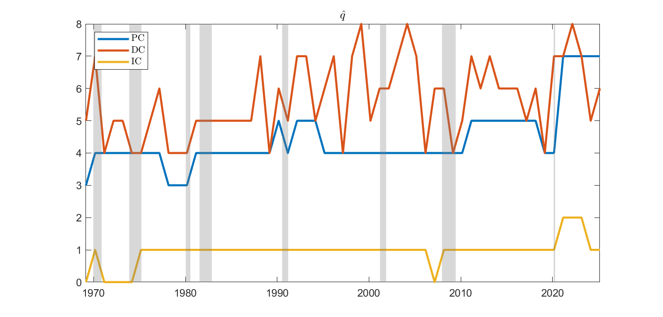
The DC2 criterion tends to select a larger number of factors, whereas the IC2 criterion typically yields a more parsimonious specification relative to the PC2 criterion. Based on the PC2 results, we find evidence in favor of four dynamic factors prior to the COVID-19 period. In contrast, the post-COVID-19 period is characterized by an increase in the estimated number of factors, with the criterion indicating the presence of seven dynamic factors.
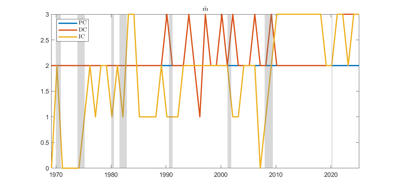
The PC2 criterion consistently selects \(m = 2\) across the sample. The DC2 criterion likewise predominantly indicates \(m = 2\) in the pre-COVID-19 period, but points to an increase to \(m = 3\) in the post-COVID-19 period. In contrast, the IC2 criterion generally favors a more parsimonious specification, selecting shorter filter lengths.
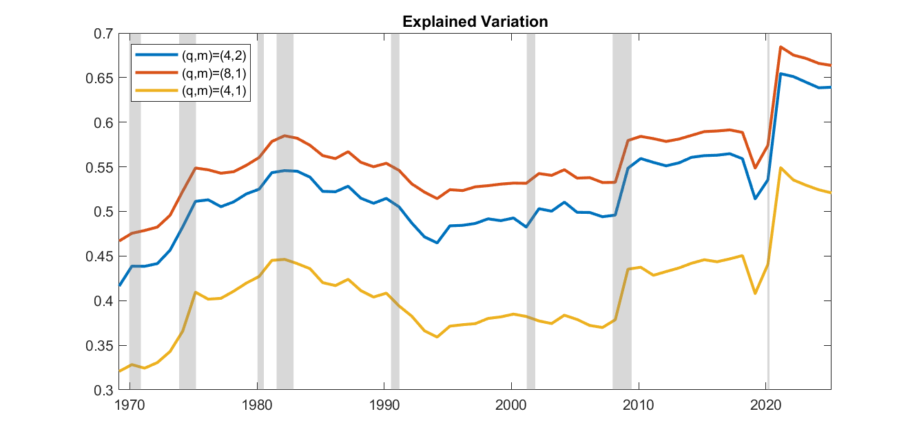
Based on the PC2 criterion, we find evidence supporting the specification \((q,m) = (4,2)\) for the majority of the sample period. The corresponding common component explains approximately 52% of the total variation in average, with this share increasing to about 65% in the post-COVID-19 period. A similar, but less drastic, increase in explained variation is also observed during the 2008 global financial crisis.
When adopting the static specification, \((q,m) = (8,1)\), the explained variation increases by approximately 3.6 percentage points. This gain can be interpreted as reflecting improved in-sample fit due to the greater flexibility of the model.
In contrast, holding the number of factors fixed while reducing the filter length to \((q,m) = (4,1)\) leads to a substantial decline in explained variation, on the order of 11.1 percentage points. This deterioration can be interpreted as evidence of misspecification.
7 Conclusion↩︎
This paper develops methods for determining the structure of dynamic factor models with finite filter length. As an intermediate step, we propose a computationally efficient alternating least squares (ALS) estimator that directly targets the dynamic factors and establish its consistency.
We introduce two procedures for jointly selecting the number of dynamic factors and filter length: a dynamic singular value ratio (DR) test extending [2], and an information criterion method similar to [1] that penalizes both the number of dynamic factors and its implied static dimensions. Both procedures are shown to be consistent.
Empirical results using the FRED-MD dataset indicate evidence of filter length \(m=2\) with four dynamic factors prior to COVID-19 period, which increase to seven post-COVID-19.
8 Appendix↩︎
Proof of Proposition [alt95spec] and Proposition [test95var] are in Supplemental Materials.
8.1 Proof of Proposition [consistency951]↩︎
Lemma 1. Let \(A,B \in \mathbb{R}^{n\times m}\). Then \[|\operatorname{tr}(A'B)|\le \operatorname{rank}(A)\,\|A\|\,\|B\|,\] where \(\|\cdot\|\) denotes the spectral norm.
Proof. Let the singular value decomposition of \(A\) be \[A = U D V',\] where \(D=\operatorname{diag}(d_1,\dots,d_r)\) with \(r=\operatorname{rank}(A)\) and \(d_i>0\). Then \[\begin{align} \operatorname{tr}(A'B)= \operatorname{tr}(V D U' B) = \operatorname{tr}(D U' B V) = \sum_{i=1}^{r} d_i\, u_i' B v_i . \end{align}\] Hence, \[|\operatorname{tr}(A'B)| \le \sum_{i=1}^{r} d_i\, |u_i' B v_i|.\] Since \(u_i\) and \(v_i\) are unit vectors and \(\|B\|\) is the spectral norm, \[|u_i' B v_i| \le \|B\|.\] Therefore, \[|\operatorname{tr}(A'B)| \le \|B\| \sum_{i=1}^{r} d_i = \|B\|\,\|A\|_*.\] Finally, since \(d_i \le \|A\|\) for all \(i\), \[\sum_{i=1}^{r} d_i \le r \|A\|,\] which yields \[|\operatorname{tr}(A'B)| \le \operatorname{rank}(A)\,\|A\|\,\|B\|.\] ◻
Proof of Proposition [consistency951]
Proof. Here, we denote \(G_0\) and \(\Gamma_0\) as the true values, e.g., \(X=G_0\Gamma_0'+E\), to distinguish them from the argument of the objective function. Consider the concentrated problem \[\begin{align} \min_{(G,\Gamma)}\frac{1}{NT}{\left\vert\kern-0.3ex\left\vert\kern-0.3ex\left\vert X-G\Gamma' \right\vert\kern-0.3ex\right\vert\kern-0.3ex\right\vert}^2 &= \min_{G}\frac{1}{NT}{\left\vert\kern-0.3ex\left\vert\kern-0.3ex\left\vert X- G(G'G)^{-1}G'X \right\vert\kern-0.3ex\right\vert\kern-0.3ex\right\vert}^2\\ &= \min_{G}\frac{1}{NT}{\left\vert\kern-0.3ex\left\vert\kern-0.3ex\left\vert (I_T- G(G'G)^{-1}G')X \right\vert\kern-0.3ex\right\vert\kern-0.3ex\right\vert}^2 \end{align}\] The objective function can be written as \[\begin{align} \frac{1}{NT}{\left\vert\kern-0.3ex\left\vert\kern-0.3ex\left\vert (I_T- G(G'G)^{-1}G')X \right\vert\kern-0.3ex\right\vert\kern-0.3ex\right\vert}^2 &= \frac{1}{NT}{\left\vert\kern-0.3ex\left\vert\kern-0.3ex\left\vert (I_T- G(G'G)^{-1}G')(G_0\Gamma_0'+E) \right\vert\kern-0.3ex\right\vert\kern-0.3ex\right\vert}^2\\ &= \frac{1}{NT}{\left\vert\kern-0.3ex\left\vert\kern-0.3ex\left\vert (I_T- G(G'G)^{-1}G')G_0\Gamma_0' \right\vert\kern-0.3ex\right\vert\kern-0.3ex\right\vert}^2\\ &+ \frac{1}{NT}{\left\vert\kern-0.3ex\left\vert\kern-0.3ex\left\vert (I_T- G(G'G)^{-1}G')E \right\vert\kern-0.3ex\right\vert\kern-0.3ex\right\vert}^2\\ &+ \frac{2}{NT}\text{tr}\left((I_T- G(G'G)^{-1}G')G_0\Gamma_0'E'\right) \end{align}\] Since \(\hat{G}\) is the minimizer of the concentrated objective function, \[\begin{align} \frac{1}{NT}{\left\vert\kern-0.3ex\left\vert\kern-0.3ex\left\vert (I_T- G_0(G_0'G_0)^{-1}G_0')X \right\vert\kern-0.3ex\right\vert\kern-0.3ex\right\vert}^2\geq\frac{1}{NT}{\left\vert\kern-0.3ex\left\vert\kern-0.3ex\left\vert (I_T- \hat{G}(\hat{G}'\hat{G})^{-1}\hat{G}')X \right\vert\kern-0.3ex\right\vert\kern-0.3ex\right\vert}^2 \end{align}\] as long as \((q,m)\in\mathcal{C}\) due to Proposition [alt95spec]. Thus, we have \[\begin{align}\label{lem0} 0&\leq\frac{1}{NT}{\left\vert\kern-0.3ex\left\vert\kern-0.3ex\left\vert (I_T- G_0(G_0'G_0)^{-1}G_0')X \right\vert\kern-0.3ex\right\vert\kern-0.3ex\right\vert}^2 -\frac{1}{NT}{\left\vert\kern-0.3ex\left\vert\kern-0.3ex\left\vert (I_T- \hat{G}(\hat{G}'\hat{G})^{-1}\hat{G}')X \right\vert\kern-0.3ex\right\vert\kern-0.3ex\right\vert}^2 \\ &=-\frac{1}{NT}{\left\vert\kern-0.3ex\left\vert\kern-0.3ex\left\vert (I_T- \hat{G}(\hat{G}'\hat{G})^{-1}\hat{G}')G_0\Gamma_0' \right\vert\kern-0.3ex\right\vert\kern-0.3ex\right\vert}^2+ \frac{1}{NT}\text{tr}\left(E'(P_{G_0}-P_{\hat{G}})E\right)\\ &-\frac{2}{NT}\text{tr}\left((I_T- \hat{G}(\hat{G}'\hat{G})^{-1}\hat{G}')G_0\Gamma_0'E'\right) \end{align}\tag{7}\] where we’ve used \[\begin{align} \frac{1}{NT}{\left\vert\kern-0.3ex\left\vert\kern-0.3ex\left\vert (I_T- G_0(G_0'G_0)^{-1}G_0')G_0\Gamma_0' \right\vert\kern-0.3ex\right\vert\kern-0.3ex\right\vert}^2&=0\\ \frac{2}{NT}\text{tr}\left((I_T- G_0(G_0'G_0)^{-1}G_0')G_0\Gamma_0'E'\right)&=0 \end{align}\] and \[\begin{align} &\frac{1}{NT}{\left\vert\kern-0.3ex\left\vert\kern-0.3ex\left\vert (I_T- G_0(G_0'G_0)^{-1}G_0')E \right\vert\kern-0.3ex\right\vert\kern-0.3ex\right\vert}^2- \frac{1}{NT}{\left\vert\kern-0.3ex\left\vert\kern-0.3ex\left\vert (I_T- G(G'G)^{-1}G')E \right\vert\kern-0.3ex\right\vert\kern-0.3ex\right\vert}^2\\ &=\frac{1}{NT}\text{tr}\left(E'(P_{G_0}-P_{\hat{G}})E\right). \end{align}\] The second term on the RHS of 7 is bounded by \[\begin{align} \left|\frac{1}{NT}\text{tr}\left(E'(P_{G_0}-P_{\hat{G}})E\right)\right| \leq \frac{1}{NT}\text{rank}(P_{G_0}-P_{\hat{G}}){\left\vert\kern-0.3ex\left\vert\kern-0.3ex\left\vert P_{G_0}-P_{\hat{G}} \right\vert\kern-0.3ex\right\vert\kern-0.3ex\right\vert}\|E\|^2, \end{align}\] due to Lemma 1. Here, \[\begin{align} {\left\vert\kern-0.3ex\left\vert\kern-0.3ex\left\vert P_{G_0}-P_{\hat{G}} \right\vert\kern-0.3ex\right\vert\kern-0.3ex\right\vert}^2 &=\text{tr}\left((P_{G_0}-P_{\hat{G}})'(P_{G_0}-P_{\hat{G}})\right)\\ &= 2\text{tr}\left(M_{\hat{G}}G_0(G_0'G_0)^{-1}G_0'\right)\\ &= 2\text{tr}\left((M_{\hat{G}}G_0)'(M_{\hat{G}}G_0)(G_0'G_0)^{-1}\right)\\ &= 2{\left\vert\kern-0.3ex\left\vert\kern-0.3ex\left\vert M_{\hat{G}}G_0 \right\vert\kern-0.3ex\right\vert\kern-0.3ex\right\vert}^2{\left\vert\kern-0.3ex\left\vert\kern-0.3ex\left\vert (G_0'G_0)^{-1} \right\vert\kern-0.3ex\right\vert\kern-0.3ex\right\vert} \end{align}\] so that \[\begin{align} {\left\vert\kern-0.3ex\left\vert\kern-0.3ex\left\vert P_{G_0}-P_{\hat{G}} \right\vert\kern-0.3ex\right\vert\kern-0.3ex\right\vert} = O_p\left(\frac{1}{\sqrt{T}}\right){\left\vert\kern-0.3ex\left\vert\kern-0.3ex\left\vert M_{\hat{G}}G_0 \right\vert\kern-0.3ex\right\vert\kern-0.3ex\right\vert}. \end{align}\] The third term on the RHS of 7 is bounded by \[\begin{align}\label{lem3} \left|\frac{2}{NT}\text{tr}\left((I_T- \hat{G}(\hat{G}'\hat{G})^{-1}\hat{G}')G_0\Gamma_0'E'\right)\right|&\leq \frac{2}{NT}{\left\vert\kern-0.3ex\left\vert\kern-0.3ex\left\vert (I_T- \hat{G}(\hat{G}'\hat{G})^{-1}\hat{G}')G_0 \right\vert\kern-0.3ex\right\vert\kern-0.3ex\right\vert}{\left\vert\kern-0.3ex\left\vert\kern-0.3ex\left\vert \Gamma_0'E' \right\vert\kern-0.3ex\right\vert\kern-0.3ex\right\vert}\\ &\leq \frac{2}{NT}{\left\vert\kern-0.3ex\left\vert\kern-0.3ex\left\vert (I_T- \hat{G}(\hat{G}'\hat{G})^{-1}\hat{G}')G_0 \right\vert\kern-0.3ex\right\vert\kern-0.3ex\right\vert}{\left\vert\kern-0.3ex\left\vert\kern-0.3ex\left\vert \Gamma_0 \right\vert\kern-0.3ex\right\vert\kern-0.3ex\right\vert}\|E\|\\ &=O_p\left(\frac{1}{\sqrt{N}}+\frac{1}{\sqrt{T}}\right)\frac{1}{\sqrt{T}}{\left\vert\kern-0.3ex\left\vert\kern-0.3ex\left\vert M_{\hat{G}}G_0 \right\vert\kern-0.3ex\right\vert\kern-0.3ex\right\vert}, \end{align}\tag{8}\] due to Assumption 2. Finally, the third term on the RHS of 7 is \[\begin{align} \frac{1}{NT}{\left\vert\kern-0.3ex\left\vert\kern-0.3ex\left\vert (I_T- \hat{G}(\hat{G}'\hat{G})^{-1}\hat{G}')G_0\Gamma_0' \right\vert\kern-0.3ex\right\vert\kern-0.3ex\right\vert}^2 &= \text{tr}\left(\left(\frac{1}{N}\Gamma_0'\Gamma_0\right)\left(\frac{1}{T}G_0'(I_T- \hat{G}(\hat{G}'\hat{G})^{-1}\hat{G}')G_0\right)\right)\\ &\geq \lambda_{min}\left(\frac{1}{N}\Gamma_0'\Gamma_0\right)\text{tr}\left(\frac{1}{T}G_0'(I_T- \hat{G}(\hat{G}'\hat{G})^{-1}\hat{G}')G_0\right)\\ &=\lambda_{min}\left(\frac{1}{N}\Gamma_0'\Gamma_0\right)\left(\frac{1}{\sqrt{T}}{\left\vert\kern-0.3ex\left\vert\kern-0.3ex\left\vert M_{\hat{G}}G_0 \right\vert\kern-0.3ex\right\vert\kern-0.3ex\right\vert}\right)^2 \end{align}\] This implies 7 can be written as \[\begin{align} 0&\leq -\text{tr}\left(\left(\frac{1}{N}\Gamma_0'\Gamma_0\right)\left(\frac{1}{T}G_0'(I_T- \hat{G}(\hat{G}'\hat{G})^{-1}\hat{G}')G_0\right)\right)\\ &+\frac{1}{NT}\text{tr}\left(E'(P_{G_0}-P_{\hat{G}})E\right)-\frac{2}{NT}\text{tr}\left((I_T- \hat{G}(\hat{G}'\hat{G})^{-1}\hat{G}')G_0\Gamma_0'E'\right)\\ &\leq -\lambda_{min}\left(\frac{1}{N}\Gamma_0'\Gamma_0\right)\left(\frac{1}{\sqrt{T}}{\left\vert\kern-0.3ex\left\vert\kern-0.3ex\left\vert M_{\hat{G}}G_0 \right\vert\kern-0.3ex\right\vert\kern-0.3ex\right\vert}\right)^2\\ &+ O_p\left(\frac{1}{N}+\frac{1}{T}\right)\frac{1}{\sqrt{T}}{\left\vert\kern-0.3ex\left\vert\kern-0.3ex\left\vert M_{\hat{G}}G_0 \right\vert\kern-0.3ex\right\vert\kern-0.3ex\right\vert}+O_p\left(\frac{1}{\sqrt{N}}+\frac{1}{\sqrt{T}}\right)\frac{1}{\sqrt{T}}{\left\vert\kern-0.3ex\left\vert\kern-0.3ex\left\vert M_{\hat{G}}G_0 \right\vert\kern-0.3ex\right\vert\kern-0.3ex\right\vert}\\ &= -\lambda_{min}\left(\frac{1}{N}\Gamma_0'\Gamma_0\right)\left(\frac{1}{\sqrt{T}}{\left\vert\kern-0.3ex\left\vert\kern-0.3ex\left\vert M_{\hat{G}}G_0 \right\vert\kern-0.3ex\right\vert\kern-0.3ex\right\vert}\right)^2+ O_p\left(\frac{1}{\sqrt{N}}+\frac{1}{\sqrt{T}}\right)\frac{1}{\sqrt{T}}{\left\vert\kern-0.3ex\left\vert\kern-0.3ex\left\vert M_{\hat{G}}G_0 \right\vert\kern-0.3ex\right\vert\kern-0.3ex\right\vert} \end{align}\] Let \(x = \frac{1}{\sqrt{T}}{\left\vert\kern-0.3ex\left\vert\kern-0.3ex\left\vert M_{\hat{G}}G_0 \right\vert\kern-0.3ex\right\vert\kern-0.3ex\right\vert}\). Since \(\lambda_{min}\left(\frac{1}{N}\Gamma_0'\Gamma_0\right)\) is strictly positive, the above equation implies \[\begin{align} x^2-O_p\left(\frac{1}{\sqrt{N}}+\frac{1}{\sqrt{T}}\right)x\leq 0 \end{align}\] Consider the second order polynomial \(f(x) = x^2-bx\). This is made negative only if \(0\leq x\leq b\). This implies that \[\begin{align} \frac{1}{\sqrt{T}}{\left\vert\kern-0.3ex\left\vert\kern-0.3ex\left\vert M_{\hat{G}}G_0 \right\vert\kern-0.3ex\right\vert\kern-0.3ex\right\vert} =\frac{1}{\sqrt{T}}{\left\vert\kern-0.3ex\left\vert\kern-0.3ex\left\vert G_0-\hat{G}(\hat{G}'\hat{G})^{-1}\hat{G}'G_0 \right\vert\kern-0.3ex\right\vert\kern-0.3ex\right\vert} = O_p\left(\frac{1}{\sqrt{N}}+\frac{1}{\sqrt{T}}\right) \end{align}\] ◻
8.2 Proof of Theorem 1 and 2↩︎
In the following Lemmas, we let \(\hat{X}_{q,m}\) be defined as \[\begin{align} \label{common95hat} \hat{X}_{q,m} = \sum_{k=0}^{m-1}\hat{F}_{-k}^{(q)}\hat{\lambda}_k^{(q)\prime} \end{align}\tag{9}\] where \((\hat{F}_{-k}^{(q)}, \hat{\lambda}_k^{(q)})_{k=0}^{m-1}\) is a minimizer of the least squares objective function given a structure \((q,m)\).
Let \(q_0\geq0,\) \(m_0\geq0\) be given, and consider disjoint partition of \(\{(q,m):0\leq q\leq q_{max}, 0\leq m\leq m_{max}\}\) given by \[\begin{align}\label{partition95set95finite} S_1&=\left\{(q,m)\in \mathbb{Z}^2 : q_0\le q\leq q_{max},\;\left\lceil \frac{q_0 m_0}{q} \right\rceil \le m \leq m_{max}\right\}\\ S_2&=\left\{(q,m)\in \mathbb{Z}^2 : m=0 \right\} \cup \left\{(q,m)\in \mathbb{Z}^2 : 1\le m<m_0,\;q<\left\lceil \frac{q_0 m_0}{m} \right\rceil \right\},\\ S_3&=\left\{(q,m)\in \mathbb{Z}^2 :m_0\leq m\le m_{max},\;q<q_0 \right\}, \end{align}\tag{10}\] where under \(q_0=0\) or \(m_0=0\) we let \(S_1=\{(q,m):0\leq q\leq q_{max}, 0\leq m\leq m_{max}\}\) and \(S_2=S_3=\emptyset\). Also, let \(\mathcal{C}=S_1\) and \(\mathcal{I}=S_2\cup S_3\).
Lemma 2. We have \[\begin{align} \hat{\delta}_{q+1,m}(X) \geq \delta_{q_0m_0+qm+1,1}(E) \end{align}\] for any \((q,m)\).
Proof. Note that we have \[\begin{align} \delta_{q+1,m}(E) \leq \left\|E-\sum_{k=0}^{m-1} F_{-k}^{(q)}\lambda_k^{(q)\prime}\right\| \end{align}\] for any matrices \((F_{-k}^{(q)},\lambda_k^{(q)})\) of conformable dimensions with \(q\) number of columns. Let \(\hat{X}_{q,m}\) be defined as in 9 . We have \[\begin{align} \hat{\delta}_{q+1,m}(X):=\|X-\hat{X}_{q,m}\| &= \left\|X-\sum_{k=0}^{m-1}\hat{F}_{-k}^{(q)}\hat{\lambda}_k^{(q)\prime}\right\|\\ &=\left\|E+\sum_{k=0}^{m_0-1}F_{-k}\lambda_k-\sum_{k=0}^{m-1}\hat{F}_{-k}^{(q)}\hat{\lambda}_k^{(q)\prime}\right\|\\ &\geq \delta_{q_0m_0+qm+1,1}(E), \end{align}\] as desired. ◻
Lemma 3. Let \(\hat{X}_{q,m}\) be defined as in 9 . Let Assumptions 1 and 2 hold. We have \[\begin{align} \frac{1}{\sqrt{NT}}{\left\vert\kern-0.3ex\left\vert\kern-0.3ex\left\vert \hat{X}_{q,m}-\sum_{k=0}^{m_0-1}F_{-k}\lambda_{-k}' \right\vert\kern-0.3ex\right\vert\kern-0.3ex\right\vert} = O_p\left(\sqrt{\frac{N+T}{NT}}\right) \end{align}\] as long as \((q,m)\in\mathcal{C}\).
Proof. Here, we denote \(G_0\) and \(\Gamma_0\) as the true values, e.g., \(X=G_0\Gamma_0'+E\), to distinguish them from the argument of the objective function. Note that we have \[\begin{align}\label{common95dev} \frac{1}{\sqrt{NT}}{\left\vert\kern-0.3ex\left\vert\kern-0.3ex\left\vert \sum_{k=0}^{m-1}\hat{F}_{-k}^{(q)}\hat{\lambda}_k^{(q)\prime}-\sum_{k=0}^{m_0-1}F_{-k}\lambda_{-k}' \right\vert\kern-0.3ex\right\vert\kern-0.3ex\right\vert} &= \frac{1}{\sqrt{NT}}{\left\vert\kern-0.3ex\left\vert\kern-0.3ex\left\vert \hat{G}\hat{\Gamma}'-G_0\Gamma_0' \right\vert\kern-0.3ex\right\vert\kern-0.3ex\right\vert}\\ &= \frac{1}{\sqrt{NT}}{\left\vert\kern-0.3ex\left\vert\kern-0.3ex\left\vert \hat{G}(\hat{G}'\hat{G})^{-1}\hat{G}'X-G_0\Gamma_0' \right\vert\kern-0.3ex\right\vert\kern-0.3ex\right\vert}\\ &= \frac{1}{\sqrt{NT}}{\left\vert\kern-0.3ex\left\vert\kern-0.3ex\left\vert \hat{G}(\hat{G}'\hat{G})^{-1}\hat{G}'G_0\Gamma_0'-G_0\Gamma_0'+\hat{G}(\hat{G}'\hat{G})^{-1}\hat{G}'E \right\vert\kern-0.3ex\right\vert\kern-0.3ex\right\vert}\\ &\leq \frac{1}{\sqrt{NT}}{\left\vert\kern-0.3ex\left\vert\kern-0.3ex\left\vert (I_T-\hat{G}(\hat{G}'\hat{G})^{-1}\hat{G}')G_0\Gamma_0' \right\vert\kern-0.3ex\right\vert\kern-0.3ex\right\vert}+\frac{1}{\sqrt{NT}}{\left\vert\kern-0.3ex\left\vert\kern-0.3ex\left\vert \hat{G}(\hat{G}'\hat{G})^{-1}\hat{G}'E \right\vert\kern-0.3ex\right\vert\kern-0.3ex\right\vert} \end{align}\tag{11}\] Here, we have \[\begin{align} \frac{1}{\sqrt{NT}}{\left\vert\kern-0.3ex\left\vert\kern-0.3ex\left\vert \hat{G}(\hat{G}'\hat{G})^{-1}\hat{G}'E \right\vert\kern-0.3ex\right\vert\kern-0.3ex\right\vert}\leq \frac{1}{\sqrt{NT}}{\left\vert\kern-0.3ex\left\vert\kern-0.3ex\left\vert \hat{G}(\hat{G}'\hat{G})^{-1}\hat{G}' \right\vert\kern-0.3ex\right\vert\kern-0.3ex\right\vert}\|E\| = O_p\left(\sqrt{\frac{N+T}{NT}}\right) \end{align}\] and \[\begin{align} \frac{1}{\sqrt{NT}}{\left\vert\kern-0.3ex\left\vert\kern-0.3ex\left\vert (I_T-\hat{G}(\hat{G}'\hat{G})^{-1}\hat{G}')G_0\Gamma_0' \right\vert\kern-0.3ex\right\vert\kern-0.3ex\right\vert} \leq \left(\frac{1}{\sqrt{T}}{\left\vert\kern-0.3ex\left\vert\kern-0.3ex\left\vert (I_T-\hat{G}(\hat{G}'\hat{G})^{-1}\hat{G}')G_0 \right\vert\kern-0.3ex\right\vert\kern-0.3ex\right\vert}\right)\left(\frac{1}{\sqrt{N}}{\left\vert\kern-0.3ex\left\vert\kern-0.3ex\left\vert \Gamma_0' \right\vert\kern-0.3ex\right\vert\kern-0.3ex\right\vert}\right) \end{align}\] so that it suffices to show \[\begin{align} \frac{1}{\sqrt{T}}{\left\vert\kern-0.3ex\left\vert\kern-0.3ex\left\vert (I_T-\hat{G}(\hat{G}'\hat{G})^{-1}\hat{G}')G_0 \right\vert\kern-0.3ex\right\vert\kern-0.3ex\right\vert} = O_p\left(\sqrt{\frac{N+T}{NT}}\right), \end{align}\] when \((q,m)\in\mathcal{C}\), which follows from Proposition [consistency951]. ◻
Lemma 4. Suppose Assumptions 1 and 2 hold. We have \[\begin{align} \frac{1}{\sqrt{NT}}\hat{\delta}_{q+1,m}(X)= O_p\left(\sqrt{\frac{N+T}{NT}}\right) \end{align}\] when \((q,m)\in\mathcal{C}\).
Proof. Let \(\hat{X}_{q,m}\) be defined as in 9 . We have \[\begin{align} \frac{1}{\sqrt{NT}}\hat{\delta}_{q+1,m}(X)&:=\frac{1}{\sqrt{NT}}\|X-\hat{X}_{q,m}\|\\ &= \frac{1}{\sqrt{NT}}\left\|E+\sum_{k=0}^{m_0-1}F_{-k}\lambda_{-k}'-\sum_{k=0}^{m-1}\hat{F}_{-k}^{(q)}\hat{\lambda}_k^{(q)\prime}\right\|\\ &\leq \frac{1}{\sqrt{NT}}\left(\|E\|+\left\|\sum_{k=0}^{m_0-1}F_{-k}\lambda_{-k}'-\sum_{k=0}^{m-1}\hat{F}_{-k}^{(q)}\hat{\lambda}_k^{(q)\prime}\right\|\right) \end{align}\] Due to Assumption 2, it suffices to show \[\begin{align} \frac{1}{\sqrt{NT}}{\left\vert\kern-0.3ex\left\vert\kern-0.3ex\left\vert \sum_{k=0}^{m_0-1}F_{-k}\lambda_{-k}'-\sum_{k=0}^{m-1}\hat{F}_{-k}^{(q)}\hat{\lambda}_k^{(q)\prime} \right\vert\kern-0.3ex\right\vert\kern-0.3ex\right\vert} = O_p\left(\sqrt{\frac{N+T}{NT}}\right), \end{align}\] which follows from Lemma 3. ◻
Lemma 5. Suppose Assumptions 1, 2, and Assumption 3 hold with \(q_0m_0+q_{max}m_{max}\leq k_{max}\). Let \((q,m)\in\mathcal{C}\). Then, for all \(\epsilon>0\), there exists \(c_0,c_1>0\) such that \[\begin{align} \mathbb{P}\left\{c_0\leq\frac{1}{\sqrt{N+T}}\hat{\delta}_{q+1,m}(X)\leq c_1\right\}\geq1-\epsilon \end{align}\] for all \(N, T\) large.
Proof. Let \(\hat{X}_{q,m}\) be defined as in 9 . Using Lemma 4, we have \(\hat{\delta}_{q+1,m}(X) = O_p(\sqrt{N+T})\) for \((q,m)\in\mathcal{C}\). Thus, for all \(\epsilon>0\), there exists \(c_1>0\) such that \[\begin{align} \mathbb{P}\left\{\frac{1}{\sqrt{N+T}}\hat{\delta}_{q+1,m}(X)> c_1\right\}\leq \epsilon/2 \end{align}\] for all \(N, T\) large and for \((q,m)\in\mathcal{C}\). Now, using Lemma 2 and Assumption 3, for all \(\epsilon>0\), there exists \(c_0>0\) such that \[\begin{align} \mathbb{P}\left\{c_0>\frac{1}{\sqrt{N+T}}\hat{\delta}_{q+1,m}(X)\right\}\leq\epsilon/2 \end{align}\] for all \(q\leq q_{max},m\leq m_{max}\) and for all \(N,T\) large. This implies \[\begin{align} \mathbb{P}\left\{c_0\leq\frac{1}{\sqrt{N+T}}\hat{\delta}_{q+1,m}(X)\leq c_1\right\}\geq 1-\epsilon, \end{align}\] for all \(N,T\) large with \((q,m)\in\mathcal{C}\). ◻
Lemma 6. Suppose Assumption 1, 2, and 4 hold. Suppose \((q,m)\in \mathcal{I}\). Then, for all \(\epsilon>0\), there exists \(c_2,c_3>0\) such that \[\begin{align} \mathbb{P}\left\{c_2 \leq \frac{1}{\sqrt{NT}}\hat{\delta}_{q+1,m}(X) \leq c_3\right\}\geq1-\epsilon \end{align}\] for all \(N,T\) large.
Proof. Let \(\hat{X}_{q,m}\) be defined as in 9 . Note that \[\begin{align} \frac{1}{\sqrt{NT}}\hat{\delta}_{q+1,m}(X):=\frac{1}{\sqrt{NT}}\|X-\hat{X}_{q,m}\| &= \frac{1}{\sqrt{NT}}\left\|E+\sum_{k=0}^{m_0-1}F_{-k}\lambda_k'-\sum_{k=0}^{m-1}\hat{F}_{-k}^{(q)}\hat{\lambda}_k^{(q)'}\right\|\\ &\leq \frac{1}{\sqrt{NT}}\left(\|E\|+\left\|\sum_{k=0}^{m_0-1}F_{-k}\lambda_k'-\sum_{k=0}^{m-1}\hat{F}_{-k}^{(q)}\hat{\lambda}_k^{(q)'}\right\|\right) \end{align}\] Here, \(\frac{1}{\sqrt{NT}}\|E\|=O_p\left(\sqrt{\frac{N+T}{NT}}\right)\) due to Assumption 2. Also, note that \[\begin{align} \frac{1}{\sqrt{NT}}\left\|\sum_{k=0}^{m_0-1}F_{-k}\lambda_k'-\sum_{k=0}^{m-1}\hat{F}_{-k}^{(q)}\hat{\lambda}_k^{(q)'}\right\|&\leq \frac{1}{\sqrt{NT}}{\left\vert\kern-0.3ex\left\vert\kern-0.3ex\left\vert \sum_{k=0}^{m_0-1}F_{-k}\lambda_k'-\sum_{k=0}^{m-1}\hat{F}_{-k}^{(q)}\hat{\lambda}_k^{(q)'} \right\vert\kern-0.3ex\right\vert\kern-0.3ex\right\vert}\\ &\leq\frac{1}{\sqrt{NT}}{\left\vert\kern-0.3ex\left\vert\kern-0.3ex\left\vert (I_T-\hat{G}(\hat{G}'\hat{G})^{-1}\hat{G}')G_0\Gamma_0' \right\vert\kern-0.3ex\right\vert\kern-0.3ex\right\vert}+\frac{1}{\sqrt{NT}}{\left\vert\kern-0.3ex\left\vert\kern-0.3ex\left\vert \hat{G}(\hat{G}'\hat{G})^{-1}\hat{G}'E \right\vert\kern-0.3ex\right\vert\kern-0.3ex\right\vert} \end{align}\] from 11 . The second term on the right hand side is bounded by \(\frac{1}{\sqrt{NT}}{\left\vert\kern-0.3ex\left\vert\kern-0.3ex\left\vert \hat{G}(\hat{G}'\hat{G})^{-1}\hat{G}' \right\vert\kern-0.3ex\right\vert\kern-0.3ex\right\vert}\|E\|=O_p\left(\sqrt{\frac{N+T}{NT}}\right)\), and the first term is bounded by \[\begin{align} \frac{1}{\sqrt{NT}}{\left\vert\kern-0.3ex\left\vert\kern-0.3ex\left\vert (I_T-\hat{G}(\hat{G}'\hat{G})^{-1}\hat{G}')G_0\Gamma_0' \right\vert\kern-0.3ex\right\vert\kern-0.3ex\right\vert} &\leq \left(\frac{1}{\sqrt{N}}{\left\vert\kern-0.3ex\left\vert\kern-0.3ex\left\vert M_{\hat{G}}G_0 \right\vert\kern-0.3ex\right\vert\kern-0.3ex\right\vert}\right)\left(\frac{1}{\sqrt{T}}{\left\vert\kern-0.3ex\left\vert\kern-0.3ex\left\vert \Gamma_0 \right\vert\kern-0.3ex\right\vert\kern-0.3ex\right\vert}\right) = O_p(1) \end{align}\] because \(\frac{1}{\sqrt{N}}{\left\vert\kern-0.3ex\left\vert\kern-0.3ex\left\vert M_{\hat{G}}G_0 \right\vert\kern-0.3ex\right\vert\kern-0.3ex\right\vert}\leq\frac{1}{\sqrt{N}}{\left\vert\kern-0.3ex\left\vert\kern-0.3ex\left\vert G_0 \right\vert\kern-0.3ex\right\vert\kern-0.3ex\right\vert}=O_p(1)\). This implies \(\frac{1}{\sqrt{NT}}\hat{\delta}_{q+1,m}(X)=O_p(1)\) so that for all \(\epsilon>0\), there exists \(c_3>0\) such that \[\begin{align} \mathbb{P}\left\{\frac{1}{\sqrt{NT}}\hat{\delta}_{q+1,m}(X) > c_3\right\}\leq\epsilon/2 \end{align}\] for all \(N,T\) large. Also, note that we have \[\begin{align}\label{lem6} \frac{1}{\sqrt{NT}}\hat{\delta}_{q+1,m}(X):=\frac{1}{\sqrt{NT}}\|X-\hat{X}_{q,m}\| &= \frac{1}{\sqrt{NT}}\left\|X-\sum_{k=0}^{m-1}\hat{F}_{-k}^{(q)}\hat{\lambda}_k^{(q)'}\right\|\\ &\geq\frac{1}{\sqrt{NT}}\left\|\sum_{k=0}^{m_0-1}F_{-k}\lambda_k'-\sum_{k=0}^{m-1}\hat{F}_{-k}^{(q)}\hat{\lambda}_k^{(q)'}\right\|-\frac{1}{\sqrt{NT}}\|E\|\\ &\geq \frac{1}{\sqrt{NT}}\delta_{q+1,m}\left(\sum_{k=0}^{m_0-1}F_{-k}\lambda_k'\right)+O_p\left(\sqrt{\frac{N+T}{NT}}\right) \end{align}\tag{12}\] Here, we’ve used reverse triangle inequality on the first inequality. The second inequality follows from the definition of \(\delta_{q+1,m}(\cdot)\) and Assumption 2. Since both \(N,T\to\infty\), we have \(O_p\left(\sqrt{\frac{N+T}{NT}}\right) = o_p(1)\). From Assumption 4, for all \(\epsilon>0\), we have \[\begin{align} \mathbb{P}\left\{c_2> \frac{1}{\sqrt{NT}}\hat{\delta}_{q+1,m}(X) \right\}\leq\epsilon/2 \end{align}\] for all \((q,m)\in S_3\) for all \(N,T\) large. For \((q,m)\in S_2\), suppose \(q_0\geq1\) and \(m_0\geq1\) because otherwise \(S_2\) is a null set. Note that we have from 12 , \[\begin{align} \frac{1}{\sqrt{NT}}\hat{\delta}_{q+1,m}(X) &\geq\frac{1}{\sqrt{NT}}\delta_{qm+1,1}(G\Gamma')+O_p\left(\sqrt{\frac{N+T}{NT}}\right), \end{align}\] and \(\frac{1}{\sqrt{NT}}\delta_{q_0m_0,1}(G\Gamma')>c\geq0\) in the limit due to Assumption 1 so that it suffices to show \(qm+1\leq q_0m_0\) for \((q,m)\in S_2\). If \(m=0\), we trivially have \(qm+1\leq q_0m_0\) because \(q_0m_0\geq 1\). If \(m>1\), we have \[qm <\left\lceil \frac{q_0 m_0}{m} \right\rceil m\leq m_0q_0,\] as desired. Thus, we have \[\begin{align} \mathbb{P}\left\{c_2\leq \frac{1}{\sqrt{NT}}\hat{\delta}_{q+1,m}(X) \leq c_3\right\}\geq1-\epsilon \end{align}\] for all \((q,m)\in \mathcal{I}\) and for all \(N,T\) large. ◻
Proof of Theorem 1
Proof. Let \(DR_{q,m}(X) = \frac{\hat{\delta}_{q,m}(X)}{\hat{\delta}_{q+1,m}(X)}\). We first consider the case where \(m_0\leq m\leq m_{max}\). For all \(\epsilon>0\), there exists \(c_4>0\) such that \[\begin{align} \mathbb{P}\left\{\frac{\frac{1}{\sqrt{NT}}\hat{\delta}_{q_0,m}(X)}{\frac{1}{\sqrt{N+T}}\hat{\delta}_{q_0+1,m}(X)}\leq c_4\right\} \leq \epsilon \end{align}\] for all \(N, T\) large. To see this, note that \[\begin{align} \mathbb{P}\left\{\frac{\frac{1}{\sqrt{NT}}\hat{\delta}_{q_0,m}(X)}{\frac{1}{\sqrt{N+T}}\hat{\delta}_{q_0+1,m}(X)}\leq \frac{c_2}{c_1}\right\} \leq \mathbb{P}\left\{\frac{1}{\sqrt{NT}}\hat{\delta}_{q_0,m}(X)\leq c_2\right\} + \mathbb{P}\left\{\frac{1}{\sqrt{N+T}}\hat{\delta}_{q_0+1,m}(X)\geq c_1\right\} \end{align}\] because \[\begin{align} \left\{\frac{1}{\sqrt{NT}}\hat{\delta}_{q_0,m}(X)>c_2\right\} \cap\left\{\frac{1}{\sqrt{N+T}}\hat{\delta}_{q_0+1,m}(X)<c_1\right\}\subset \left\{\frac{\frac{1}{\sqrt{NT}}\hat{\delta}_{q_0,m}(X)}{\frac{1}{\sqrt{N+T}}\hat{\delta}_{q_0+1,m}(X)}>\frac{c_2}{c_1}\right\}. \end{align}\] We use Lemma 5 and Lemma 6 with \(\epsilon/2\) and take \(c_4=\frac{c_2}{c_1}\) to finish. This implies \(\frac{\frac{1}{\sqrt{NT}}\hat{\delta}_{q_0,m}(X)}{\frac{1}{\sqrt{N+T}}\hat{\delta}_{q_0+1,m}(X)}\) is strictly positive with probability approaching one as \(N,T\to\infty\). Note that \[\begin{align} DR_{q_0,m}(X) &= \frac{\hat{\delta}_{q_0,m}(X)}{\hat{\delta}_{q_0+1,m}(X)}\\ &= \left(\frac{\sqrt{NT}}{\sqrt{N+T}}\right)\frac{\hat{\delta}_{q_0,m}(X)}{\frac{1}{\sqrt{N+T}}\hat{\delta}_{q_0+1,m}(X)} \end{align}\] Thus, for all \(\epsilon>0\), there exists \(c_4>0\) such that \[\begin{align} \mathbb{P}\left\{DR_{q_0,m}(X)>\left(\frac{\sqrt{NT}}{\sqrt{N+T}}\right)c_4\right\}\geq 1-\epsilon \end{align}\] for all \(N,T\) large. This implies that \(DR_{q_0,m}(X)\) is stochastically unbounded as \(N,T\to\infty\). Also, using Lemma 5, for all \(q=q_0+1,\ldots,q_{max}\) and for all \(\epsilon>0\), there exists \(c_0\) and \(c_1\) such that \[\begin{align} \mathbb{P}\left\{DR_{q,m}(X) \geq \frac{c_1}{c_0}\right\} \leq \epsilon \end{align}\] for all \(N+T\) large. To see this, note that \[\begin{align} \left\{\frac{1}{\sqrt{N+T}}\hat{\delta}_{q,m}(X)< c_1\right\}\cap \left\{\frac{1}{\sqrt{N+T}}\hat{\delta}_{q+1,m}(X) > c_0\right\}\subset\left\{\frac{\frac{1}{\sqrt{N+T}}\hat{\delta}_{q,m}(X)}{\frac{1}{\sqrt{N+T}}\hat{\delta}_{q+1,m}(X)} < \frac{c_1}{c_0}\right\} \end{align}\] This implies \(DR_{q,m}(X)\) is stochastically bounded for all \(q=q_0+1,\ldots,q_{max}\) as \(N,T\to\infty\). Similarly, using Lemma 6, we may show that \(DR_{q,m}(X)\) is stocastically bounded for all \(q=1,\ldots,q_0-1\) as \(N,T\to\infty\). This implies that \[\begin{align} \mathbb{P}\left\{\hat{q} = q_0\right\} \to1 \end{align}\] as \(N,T\to\infty\).
The proof for the case \(m<m_0\) follows similarly. Using Lemma 5 and Lemma 6, \(\frac{1}{\sqrt{N+T}}\hat{\delta}_{q+1,m}(X)\) is asymptotically strictly positive and bounded for \(q=\left\lceil \frac{q_0m_0}{m}\right\rceil,\ldots,q_{max}\) and \(\frac{1}{\sqrt{NT}}\hat{\delta}_{q+1,m}(X)\) is asymptotically strictly positive and bounded for \(q=1,\ldots,\left\lceil \frac{q_0m_0}{m}\right\rceil-1\). These imply that the ratio \(DR_{q,m}(X)=\frac{\hat{\delta}_{q,m}(X)}{\hat{\delta}_{q+1,m}(X)}\) is stochastically bounded for all \(q=1,\ldots,\left\lceil \frac{q_0m_0}{m}\right\rceil-1\) and \(q=\left\lceil \frac{q_0m_0}{m}\right\rceil+1,\ldots,q_{max}\). The ratio \(DR_{q,m}(X)=\frac{\hat{\delta}_{q,m}(X)}{\hat{\delta}_{q+1,m}(X)}\) diverges with probability approaching one only at \(q=\left\lceil \frac{q_0m_0}{m}\right\rceil\). ◻
Proof of Theorem 2
Proof. We let \(DR_{q,m}(X) = \frac{\hat{\delta}_{q+1,m-1}(X)}{\hat{\delta}_{q+1,m}(X)}\). Suppose \(q=q_0\). Using Lemma 5 and Lemma 6, \(\frac{1}{\sqrt{N+T}}\hat{\delta}_{q_0+1,m}(X)\) is asymptotically strictly positive and bounded for all \(m_0\leq m\leq m_{max}\) and \(\frac{1}{\sqrt{NT}}\hat{\delta}_{q_0+1,m}(X)\) is strictly positive for \(m\leq m_0-1\). Thus, \(DR_{q_0,m}(X)\) diverges with probability approaching one only when \(m=m_0\) and stays stochastically bounded otherwise.
Now suppose \(q>q_0\). Note that \(\frac{1}{\sqrt{N+T}}\hat{\delta}_{q+1,m}(X)\) is asymptotically strictly positive and bounded for \(m=\left\lceil\frac{q_0m_0}{q}\right\rceil,\ldots,m_{max}\) due to Lemma 5. Also, \(\frac{1}{\sqrt{NT}}\hat{\delta}_{q+1,m}(X)\) is asymptotically strictly positive and bounded for \(m=1,\ldots,\left\lceil\frac{q_0m_0}{q}\right\rceil-1\) due to Lemma 6. Thus, \(DR_{q,m}(X)\) diverges with probability approaching one only when \(m=\left\lceil\frac{q_0m_0}{q}\right\rceil\) and stays stochastically bounded otherwise. ◻
8.3 Proof of Theorem 3↩︎
Lemma 7. Suppose Assumptions 1, 2, and 4 hold. We have \[V(q_0,m_0)-V(q,m) = O_p\left(\frac{N+T}{NT}\right)\] when \((q,m)\in\mathcal{C}\). Also, for all \(\epsilon>0\), there exists \(c>0\) such that \[\mathbb{P}\left\{V(q,m)-V(q_0,m_0) \geq c\right\}\geq 1-\epsilon\] for all \(N,T\) large when \((q,m)\in\mathcal{I}\).
Proof. From \[\begin{align} V(q,m) &= \frac{1}{NT}{\left\vert\kern-0.3ex\left\vert\kern-0.3ex\left\vert \sum_{k=0}^{m-1}\hat{F}_{-k}^{(q)}\hat{\lambda}_k^{(q)\prime}-\sum_{k=0}^{m_0-1}F_{-k}\lambda_{-k}' \right\vert\kern-0.3ex\right\vert\kern-0.3ex\right\vert}^2 + \frac{1}{NT}{\left\vert\kern-0.3ex\left\vert\kern-0.3ex\left\vert E \right\vert\kern-0.3ex\right\vert\kern-0.3ex\right\vert}^2\\ &- \frac{2}{NT}\text{tr}\left(\left(\sum_{k=0}^{m-1}\hat{F}_{-k}^{(q)}\hat{\lambda}_k^{(q)\prime}-\sum_{k=0}^{m_0-1}F_{-k}\lambda_{-k}'\right)'E\right), \end{align}\] we have \[\begin{align}\label{V95diff} V(q_0,m_0)-V(q,m) &= \frac{1}{NT}{\left\vert\kern-0.3ex\left\vert\kern-0.3ex\left\vert \sum_{k=0}^{m_0-1}\hat{F}_{-k}^{(q_0)}\hat{\lambda}_k^{(q_0)}-\sum_{k=0}^{m_0-1}F_{-k}\lambda_{-k}' \right\vert\kern-0.3ex\right\vert\kern-0.3ex\right\vert}^2-\frac{1}{NT}{\left\vert\kern-0.3ex\left\vert\kern-0.3ex\left\vert \sum_{k=0}^{m-1}\hat{F}_{-k}^{(q)}\hat{\lambda}_k^{(q)\prime}-\sum_{k=0}^{m_0-1}F_{-k}\lambda_{-k}' \right\vert\kern-0.3ex\right\vert\kern-0.3ex\right\vert}^2\\ &-\frac{2}{NT}\text{tr}\left(\left(\sum_{k=0}^{m_0-1}\hat{F}_{-k}^{(q_0)}\hat{\lambda}_k^{(q_0)}-\sum_{k=0}^{m_0-1}F_{-k}\lambda_{-k}'\right)'E\right)\\ &+\frac{2}{NT}\text{tr}\left(\left(\sum_{k=0}^{m-1}\hat{F}_{-k}^{(q)}\hat{\lambda}_k^{(q)\prime}-\sum_{k=0}^{m_0-1}F_{-k}\lambda_{-k}'\right)'E\right). \end{align}\tag{13}\] Also, we have \[\begin{align} \label{cross95diff} \frac{1}{NT}\text{tr}\left(\left(\sum_{k=0}^{m-1}\hat{F}_{-k}^{(q)}\hat{\lambda}_k^{(q)\prime}-\sum_{k=0}^{m_0-1}F_{-k}\lambda_{-k}'\right)'E\right) \leq \frac{mq+m_0q_0}{NT}{\left\vert\kern-0.3ex\left\vert\kern-0.3ex\left\vert \sum_{k=0}^{m-1}\hat{F}_{-k}^{(q)}\hat{\lambda}_k^{(q)\prime}-\sum_{k=0}^{m_0-1}F_{-k}\lambda_{-k}' \right\vert\kern-0.3ex\right\vert\kern-0.3ex\right\vert}\|E\|. \end{align}\tag{14}\] If \((q,m)\in\mathcal{C}\), the right hand side of equation 13 is \(O_p\left(\frac{N+T}{NT}\right)\) due to Lemma 3, equation 14 , and Assumption 2.
Now, if \((q,m)\in\mathcal{I}\), we have \(\frac{1}{NT}{\left\vert\kern-0.3ex\left\vert\kern-0.3ex\left\vert \sum_{k=0}^{m-1}\hat{F}_{-k}^{(q)}\hat{\lambda}_k^{(q)\prime}-\sum_{k=0}^{m_0-1}F_{-k}\lambda_{-k}' \right\vert\kern-0.3ex\right\vert\kern-0.3ex\right\vert}^2\) strictly positive in the limit. To see this, \[\begin{align} \frac{1}{\sqrt{NT}}{\left\vert\kern-0.3ex\left\vert\kern-0.3ex\left\vert \sum_{k=0}^{m-1}\hat{F}_{-k}^{(q)}\hat{\lambda}_k^{(q)\prime}-\sum_{k=0}^{m_0-1}F_{-k}\lambda_{-k}' \right\vert\kern-0.3ex\right\vert\kern-0.3ex\right\vert} &\geq \frac{1}{\sqrt{NT}}\left\|\sum_{k=0}^{m-1}\hat{F}_{-k}^{(q)}\hat{\lambda}_k^{(q)\prime}-\sum_{k=0}^{m_0-1}F_{-k}\lambda_{-k}'\right\|\\ &=\frac{1}{\sqrt{NT}}\delta_{q+1,m}\left(\sum_{k=0}^{m_0-1}F_{-k}\lambda_{-k}'\right), \end{align}\] which is strictly positive in the limit as shown in Lemma 6. ◻
Proof of Theorem 3
Proof. We show that \[\mathbb{P}\{PC(q,m)<PC(q_0,m_0)\}\to 0\] as \(N,T\to\infty\) for all \(q\leq q_{max}\) and \(m\leq m_{max}\) such that both \(q\neq q_0\) and \(m\neq m_0\). Using Lemma 7, for all \(\epsilon>0\), there exists \(c>0\) such that \[\mathbb{P}\left\{V(q,m)-V(q_0,m_0) \geq c\right\}\geq 1-\epsilon\] for all \(N,T\) large when \((q,m)\in\mathcal{I}\). Note that we have \[PC(q,m)-PC(q_0,m_0) = V(q,m)-V(q_0,m_0) -(r_0+q_0-(r+q))g(N,T),\] where the first term \(V(q,m)-V(q_0,m_0)\) is strictly positive in the limit, whereas the second term \((r_0+q_0-(r+q))g(N,T)\) vanishes. Thus, we have \(\mathbb{P}\{PC(q,m)<PC(q_0,m_0)\}\to 0\) when \((q,m)\in\mathcal{I}\).
Also, using Lemma 7, we have \[V(q_0,m_0)-V(q,m) = O_p\left(\frac{N+T}{NT}\right)\] when \((q,m)\in\mathcal{C}\). Note that we may write \[\mathbb{P}\{PC(q,m)<PC(q_0,m_0)\}=\mathbb{P}\{V(q_0,m_0)-V(q,m) >(r+q-(r_0+q_0))g(N,T)\},\] where the left hand side vanishes at the order \(O_p\left(\frac{N+T}{NT}\right)\) and the right hand side vanishes at a slower rate. Note that any \((q,m)\in\mathcal{C}\) such that \((q,m)\neq (q_0,m_0)\) gives \(r+q>r_0+q_0\) so that \(\mathbb{P}\{PC(q,m)<PC(q_0,m_0)\}\to 0\) when \((q,m)\in\mathcal{C}\) but \((q,m)\neq(q_0,m_0)\).
For \(DC(q,m)\), note that we have \[\frac{1}{NT}\hat{\delta}^2_{q+1,m}(X) = O_p\left(\frac{N+T}{NT}\right)\] when \((q,m)\in\mathcal{C}\) due to Lemma 5. Note that in using Lemma 5, we only use the stochastic boundedness so that Assumption 3 is not needed. Also, for all \(\epsilon>0\), there exists \(c>0\) such that \[\begin{align} \mathbb{P}\left\{\frac{1}{\sqrt{NT}}\hat{\delta}^2_{q+1,m}(X) \geq c\right\}\geq1-\epsilon \end{align}\] when \((q,m)\in\mathcal{I}\) due to Lemma 6. Since \(\frac{1}{NT}\hat{\delta}^2_{q_0+1,m_0}(X)=O_p\left(\frac{N+T}{NT}\right)\), we may use the same argument as in the case of \(PC(q,m)\) to finish. ◻
9 Supplemental Materials for "Determining the Structure of Dynamic Factor Models"↩︎
by Sangmyung Ha
9.1 Proof of Proposition [alt95spec]↩︎
Proof. We give a proof by construction. We first consider the representations with the number of factors and filter length given by \((\left\lceil\frac{q_0m_0}{m}\right\rceil,m)\) for \(1\leq m< m_0\).
Suppose \(\frac{q}{q_0}\) is an integer. The common component of the original representation is given by \(\sum_{k=0}^{m_0-1}\lambda_kf_{t-k}\). Let \(\sum_{k=0}^{m-1}\Gamma_kg_{t-k}\) be a candidate representation with \(\Gamma_k\in\mathbb{R}^{N\times q}\) and \(g_t\in\mathbb{R}^{q}\) where \(q=\lceil\frac{q_0m_0}{m}\rceil\). We may construct \(g_t\) and \(\Gamma_k\) as \[g_t = \begin{pmatrix} f_t\\ f_{t-m}\\ \vdots\\ f_{t-(\frac{q}{q_0}-1)m} \end{pmatrix}, \Gamma_k = \begin{pmatrix} \lambda_{k} & \lambda_{k+m} & \ldots &\lambda_{k+(\frac{q}{q_0}-1)m} \end{pmatrix},\] where we define \(\lambda_{k}=0\) for \(k> m_0\). The vector \(g_t\) collects \(\frac{q}{q_0}\) number of \(f_t\) so that \(g_t\in\mathbb{R}^{q}\). By constructing \(g_t\) and \(\Gamma_k\) in this way, we see that \[\begin{align} \sum_{k=0}^{m-1}\Gamma_kg_{t-k} &= \sum_{k=0}^{m-1}\left(\lambda_kf_{t-k} + \lambda_{k+m}f_{t-k-m} + \ldots +\lambda_{k+(\frac{q}{q_0}-1)m}f_{t-k-(\frac{q}{q_0}-1)m}\right). \end{align}\] The first term on the right hand side accounts for \(\lambda_kf_{t-k},\) with \(k=0,\ldots m-1\). The second term accounts for \(k=m,\ldots,2m-1\) and so on. The final term accounts for \(k=(\frac{q}{q_0}-1)m,\ldots,m-1+(\frac{q}{q_0}-1)m\). Here, we see that the index for the final term satisfies \[\begin{align} m-1+(\frac{q}{q_0}-1)m = \frac{qm}{q_0}-1\geq m_0-1, \end{align}\] since \(\frac{q_0m_0}{m}\leq q\). Thus, \(\sum_{k=0}^{m-1}\Gamma_kg_{t-k} = \sum_{k=0}^{m_0-1}\lambda_kf_{t-k}\).
Now, we consider the case where \(\frac{q}{q_0}\) is not an integer. Let \(\sum_{k=0}^{m-1}\Gamma_kg_{t-k}\) be a candidate representation with \(\Gamma_k\in\mathbb{R}^{N\times q}\) and \(g_t\in\mathbb{R}^{q}\) where \(q=\left\lceil\frac{q_0m_0}{m}\right\rceil\). We first consider \(g_t\) constructed as \[g_t = \begin{pmatrix} f_t\\ f_{t-m}\\ \vdots\\ f_{t-(\lceil\frac{q}{q_0}\rceil-2)m}\\ 0_{(q-(\lceil\frac{q}{q_0}\rceil-1) q_0)\times 1} \end{pmatrix} + \begin{pmatrix} 0_{(q-q_0)\times 1}\\ f_{t-m_0+m} \end{pmatrix}\] Note that \(g_t\in\mathbb{R}^q\) because \(q_0(\lceil\frac{q}{q_0}\rceil-1)+(q-(\lceil\frac{q}{q_0}\rceil-1) q_0) = q\) and \(q>(\lceil\frac{q}{q_0}\rceil-1) q_0\). Also, we have \(\lceil\frac{q}{q_0}\rceil = \lceil\frac{m_0}{m}\rceil\). To see this, by definition of the ceiling, we have \(\frac{q_0m_0}{m}\leq q_0\lceil\frac{m_0}{m}\rceil\), which implies \[\begin{align} q\leq q_0\lceil\frac{m_0}{m}\rceil \end{align}\] because \(q_0\lceil\frac{m_0}{m}\rceil\) is an integer. Thus, \(\frac{q}{q_0}\leq \lceil\frac{m_0}{m}\rceil\), combined with \(\frac{q_0m_0}{m}\leq q\) implies \[\begin{align} \frac{m_0}{m}\leq \frac{q}{q_0} \leq \lceil\frac{m_0}{m}\rceil. \end{align}\] Given the definition of \(g_t\), we may show that all the elements in \(f_{t-k},k=0,\ldots,m_0-1\) appear in \(g_{t-k},k=0,\ldots,m-1\) either alone, or as a sum. Note that first term of the right-hand side accounts for \(f_{t-k},k=0,\ldots,(\lceil\frac{m_0}{m}\rceil-1)m-1\). The second term accounts for \(f_{t-k},k=m_0-m,\ldots,m_0-1\). Here, we have \((\lceil\frac{m_0}{m}\rceil-1)m > m_0-m\) so that all of \(f_{t-k},k=1,\ldots,m_0\) are accounted for. Also, \(q-(\lceil\frac{q}{q_0}\rceil-1) q_0=q-\lfloor\frac{q}{q_0}\rfloor q_0<q_0\) because the left hand side of the inequality is the remainder when dividing \(q\) by \(q_0\). This means that some elements of \(g_{t-k}\) consists of sum of two elements in \((f_{t-k})\). We first consider the top \((\lceil\frac{q}{q_0}\rceil-2)\) blocks of \(g_t\), i.e, \((f_{t-k}),k=0,m,\ldots,(\lceil\frac{q}{q_0}\rceil-3)\). These elements do not appear as a sum and do not appear as elements in other \((g_{t-k}),k=1,\ldots,m-1\). This implies that we may construct the left \((\lceil\frac{q}{q_0}\rceil-2)\) block of \(\Gamma_k\) as \(\begin{pmatrix} \lambda_{k} & \lambda_{k+m} & \ldots &\lambda_{k+(\lceil\frac{q}{q_0}\rceil-3)m} \end{pmatrix}\) for \(k=0,\ldots,m-1\) so that the top \((\lceil\frac{q}{q_0}\rceil-2)\) blocks of \((g_{t-k})\), together with the given construction of \((\Gamma_k)\), accounts for \((\lambda_kf_{t-k})_{k=0}^{(\lceil\frac{q}{q_0}\rceil-2)m-1}\). By constructing the top \((\lceil\frac{q}{q_0}\rceil-2)\) block of \(g_t\) in this way, we see that it suffices to show that the alternative dynamic factor representation \((\left\lceil\frac{q_0m_0}{m}\right\rceil,m)\) holds for \((q_0,m_0)\) where \(\lceil \frac{q}{q_0}\rceil=2\). We first consider the case with \(q-q_0=m_0-m\). Suppose \(q-q_0=m_0-m\). We may construct \(g_t\) as \[g_{t-k} = \begin{pmatrix} f_{t-k}\\ 0_{(q-q_0)\times 1}\\ \end{pmatrix}+\begin{pmatrix} 0\\ f_{t-(k+1)}\\ 0_{(q-q_0-1)\times 1}\\ \end{pmatrix}+\ldots\begin{pmatrix} 0_{(q-q_0)\times 1}\\ f_{t-(m_0-m)} \end{pmatrix},\] where we sum over \(q-q_0\) number of \((f_{t-k})\) while performing cyclic permutation and adding lags. For example, suppose we want to represent a dynamic factor model with \((q_0,m_0)=(3,5)\) as a model with \((q,m) = (5,3)\). We can define \(g_{t-k}\) as \[g_{t-k} = \begin{pmatrix} f_{t-k,1}\\ f_{t-k,2}\\ f_{t-k,3}\\ 0\\ 0\\ \end{pmatrix}+\begin{pmatrix} 0\\ f_{t-(k+1),1}\\ f_{t-(k+1),2}\\ f_{t-(k+1),3}\\ 0\\ \end{pmatrix}+\begin{pmatrix} 0\\ 0\\ f_{t-(k+2),1}\\ f_{t-(k+2),2}\\ f_{t-(k+2),3}\\ \end{pmatrix}\] Note that all of \((f_{t-k}),k=0,\ldots,m_0-1\) are included in \((g_{t-k}),k=0,\ldots,m-1\). Also, each elements in \((f_{t-k}),k=0,\ldots,m_0-1\) exists in \((g_{t-k})\) either alone, e.g., \(f_{t-k,1}\) and \(f_{t-(k+2),3}\), or as a sum over other elements in \((f_{t-k})\). The key observation here is that each element in \((f_{t-k}),k=0,\ldots,m_0-1\) appears in \((g_{t-k})\) as a collection of groups whose number of unique elements match the number of groups in each collection. This implies that we may solve for \((\Gamma_k)\) such that \(\sum_{k=0}^{m-1}\Gamma_kg_{t-k} =\sum_{k=0}^{m_0-1}\lambda_kf_{t-k}\). This can be done for any \((q_0,m_0)\) and \((q,m)\) as long as \(q-q_0 = m_0-m\).
Now, consider the general case where \(q-q_0\) may not equal \(m_0-m\). For this general case, the way that we can solve for \((\Gamma_k)\) given \((g_{t-k})\) to satisfy \(\sum_{k=0}^{m-1}\Gamma_kg_{t-k} =\sum_{k=0}^{m_0-1}\lambda_kf_{t-k}\) is the same. The solution exists whenever elements in \((g_{t-k})\) can be formed into collections whose number of groups is larger than the number of unique elements of \((f_{t-k})\) appearing in the collection. We may always construct \((g_{t-k})\) in a way such that we only have one collection, whose number of groups are given by \(qm\), which is greater than or equal to the number of unique elements in \((f_{t-k})\), i.e., \(q_0m_0\).
Now, it is left to show that Assumption 1 ensures that the bounds are sharp. When \(m<m_0\), the dynamic model cannot be written with the structure \[(q, m) = \left( \left\lceil \frac{q_0 m_0}{m} \right\rceil-1, m \right),\] because positive definiteness of \(\frac{1}{T}G'G\) and \(\frac{1}{N}\Gamma'\Gamma\) requires at least \(r=q_0m_0\) vectors to match \(G\Gamma'\), where \(G\) and \(\Gamma\) are defined as in Assumption 1. Note that the structure \((q, m) = \left( \left\lceil \frac{q_0 m_0}{m} \right\rceil-1, m \right)\) implies using \[\begin{align} \left( \left\lceil \frac{q_0 m_0}{m} \right\rceil-1\right)m = \begin{cases} q_0m_0-m & \text{if \frac{q_0m_0}{m} is an integer}\\ \left\lfloor \frac{q_0 m_0}{m} \right\rfloor m<q_0m_0 & \text{if \frac{q_0m_0}{m} is not an integer} \end{cases} \end{align}\] number of vectors to match \(G\Gamma'\), which is strictly less than \(q_0m_0\) as long as \(m\geq1\).
The representations with the number of factors and filter length given by \((q,\lceil \frac{q_0m_0}{q}\rceil)\) for \(q>q_0\) can be shown in the same way as in the case with \((\left\lceil\frac{q_0m_0}{m}\right\rceil,m)\) for \(1\leq m< m_0\). ◻
9.2 Proof of Proposition [test95var]↩︎
Before proving Proposition [test95var], we first prove that the estimated dynamic factors \((f_t)\) are consistent up to a \(q\times q\) dimensional invertible matrix.
Lemma 8. Let Assumption 1 hold. Then, we have \[\begin{align} \left\|\left(\sum_{j,k=0}^{m-1}(P_{j-k}\otimes \frac{1}{N}\lambda_j'\lambda_k)\right)^{-1}\right\| = O_p(1) \end{align}\]
Proof. It suffices to show that the smallest eigenvalue of the matrix \(S\) defined as \[\begin{align} S = \sum_{j,k=0}^{m-1}\left(P_{j-k}\otimes \frac{1}{N}\lambda_j'\lambda_k\right) \end{align}\] is bounded away from zero. Defining the lag-\(h\) block as \[\begin{align} B_h = \frac{1}{N}\sum_{k=0}^{m-1}\lambda_{k+h}'\lambda_k, \quad h=j-k, \end{align}\] we may write \[\begin{align} S = \sum_{h=-(m-1)}^{m-1}(P_h\otimes B_h) \end{align}\] with the convention that \(\lambda_k = 0\) for \(k<0\) and \(k>m-1\). Let \(a=(a_1',\ldots,a_{T+m-1}')'\) be \((T+m-1)q\) dimensional vector with \(q\) dimensional blocks given by \((a_t)\). Consider the \(t\)-th block of the product \(Sa\). For a single Kronecker term, we have \[\begin{align} ((P_h\otimes B_h)a)_t = \sum_{s=1}^{T+m-1}(P_h)_{t,s}B_ha_s. \end{align}\] Here, \(P_h\) is the cyclic shift by \(-h\), meaning \((P_h)_{t,s}=1\) if and only if \(s=t+h\) modulo \(T+m-1\). Therefore, \[\begin{align} ((P_h\otimes B_h)a)_t = B_ha_{t+h} \end{align}\] Here and after, the time indices on \((a_t)\) are defined with modulo \(T+m-1\). Summing over \(h\) gives \[\begin{align} (Sa)_t = \sum_{h=-(m-1)}^{m-1}B_ha_{t+h} \end{align}\] This is a convolution in the time index \(t\), where each output block at time \(t\) is given by a convolution of the sequence \((B_{-h})\) with the sequence \((a_t)\).
We may define the blockwise discrete Fourier transform for frequencies \(\omega_\ell = 2\pi l/(T+m-1),l=1,\ldots,T+m-1\), \[\begin{align} a(\omega_\ell) = \sum_{t=1}^{T+m-1}a_t e^{-i\omega_{\ell}t}, \end{align}\] which give a \(q\)-vector for each \(l=1,\ldots,T+m-1\). Applying the same transform to the output sequence \(b_t=(Sa)_t\), we obtain \[\begin{align} b(\omega_{\ell}) = \sum_{t=1}^{T+m-1}b_te^{-i\omega_{\ell}t} = \sum_{t=1}^{T+m-1}\left(\sum_{h=-(m-1)}^{m-1}B_ha_{t+h}\right)e^{-i\omega_{\ell}t}. \end{align}\] Changing the summation order and the time index \(s=t+h\), we obtain \[\begin{align} b(\omega_{\ell}) &= \sum_{h=-(m-1)}^{m-1}B_h\sum_{s=1}^{T+m-1}a_se^{-i\omega_{\ell}(s-h)} = \left(\sum_{h=-(m-1)}^{m-1}B_he^{i\omega_{\ell} h}\right)a(\omega_{\ell}) \end{align}\] Thus, \[\begin{align} b(\omega_{\ell}) = B(e^{i\omega_{\ell}})a(\omega_{\ell}) \end{align}\] with \[\begin{align} B(e^{i\omega}) = \sum_{h=-(m-1)}^{m-1}B_he^{i\omega h} \end{align}\] This implies that the DFT diagonalizes the matrix multiplications where the action of \(S\) is reduced to frequency-by-frequency multiplication by a \(q\times q\) matrix \(B(e^{i\omega})\). Let a phase vector \(v(\omega)\) be defined as \[\begin{align} v(\omega) := (e^{-i\omega 0},\dots,e^{-i\omega (m-1)})' \in \mathbb{C}^{m}. \end{align}\] Note that we have \[\begin{align} B(e^{i\omega}) &= \sum_{h=-(m-1)}^{m-1}B_he^{i\omega h}= \frac{1}{N}\sum_{h=-(m-1)}^{m-1}\sum_{k=0}^{m-1}\lambda_{k+h}'\lambda_ke^{i\omega h}= \frac{1}{N}\sum_{j,k=0}^{m-1}\lambda_{j}'\lambda_ke^{i\omega (j-k)}\\ &= (v(\omega)\otimes I_q)'\left(\frac{1}{N}\Gamma'\Gamma\right)(v(\omega)\otimes I_q) \end{align}\] By Assumption 1, \[\begin{align} \frac{1}{N}\Gamma'\Gamma &\to_p M_\gamma >0 \end{align}\] Let the smallest eigenvalue of \(M_\gamma\) be given by \(c_0>0\). For every \(\omega\), we have \[\begin{align} B(e^{i\omega}) = (v(\omega)\otimes I_q)' \Big(\frac{1}{N} \Gamma'\Gamma \Big) (v(\omega)\otimes I_q) \geq c_0(v(\omega)\otimes I_q)' (v(\omega)\otimes I_q). \end{align}\] for \(N,T\) large, where \(E\geq F\) is used to denote \(E-F\) is positive semi-definite. Since each entry of \(v(\omega)\) has modulus \(1\) and there are \(m\) entries, \[(v(\omega)\otimes I_q)'(v(\omega)\otimes I_q) = mI_q.\] Therefore, \[B(e^{i\omega}) \geq c_0 m \, I_q > 0 \quad \text{for all } \omega.\] Finally, because the DFT is unitary, the smallest eigenvalue of \(S\) is bounded below by \(c_0m\). To see this, note that \[\begin{align} \|Sa\|^2 = \sum_{\ell=1}^{T+m-1}\|b(\omega_{\ell})\|^2&= \sum_{\ell=1}^{T+m-1}\|B(e^{i\omega_{\ell}})a(\omega_{\ell})\|^2\\ &\geq c_0m\sum_{\ell=1}^{T+m-1}\|a(\omega_{\ell})\|^2= c_0m\|a\|^2. \end{align}\] ◻
Let Assumptions 1, 2, and 5 hold. Let \(\hat{F}\) and \((\hat{\lambda}_k)\) be a minimizer the objective function 4 . Then, we have \[\begin{align} \frac{1}{\sqrt{T}}{\left\vert\kern-0.3ex\left\vert\kern-0.3ex\left\vert \hat{F}-FH_f' \right\vert\kern-0.3ex\right\vert\kern-0.3ex\right\vert} &= O_p\left(\frac{1}{\sqrt{T}}+\frac{1}{\sqrt{N}}\right)\\ \frac{1}{\sqrt{N}}{\left\vert\kern-0.3ex\left\vert\kern-0.3ex\left\vert \hat{\lambda}_k-\lambda_kH_f^{-1} \right\vert\kern-0.3ex\right\vert\kern-0.3ex\right\vert} &= O_p\left(\frac{1}{\sqrt{T}}+\frac{1}{\sqrt{N}}\right),\quad k=0,\ldots,m-1 \end{align}\] where \(H_f \in \mathbb{R}^{q \times q}\) is defined as \[\begin{align} H_f = \left(\sum_{k=0}^{m-1}\lambda_k'\hat{\lambda}_k\right)\left(\sum_{k=0}^{m-1}\hat{\lambda}_k'\hat{\lambda}_k\right)^{-1}. \end{align}\]
Proof. Proposition [consistency951] implies that \[\begin{align} \frac{1}{\sqrt{N}}{\left\vert\kern-0.3ex\left\vert\kern-0.3ex\left\vert \hat{\Gamma} - \Gamma H_\gamma' \right\vert\kern-0.3ex\right\vert\kern-0.3ex\right\vert} &= O_p\Big(\frac{1}{\sqrt{N}} + \frac{1}{\sqrt{T}}\Big),\\ \frac{1}{\sqrt{T}}{\left\vert\kern-0.3ex\left\vert\kern-0.3ex\left\vert \hat{G} - GH_\gamma^{-1} \right\vert\kern-0.3ex\right\vert\kern-0.3ex\right\vert} &= O_p\Big(\frac{1}{\sqrt{N}} + \frac{1}{\sqrt{T}}\Big), \end{align}\] where \(H_\gamma \in \mathbb{R}^{mq \times mq}\) is defined by \[H_\gamma = (\hat{G}' \hat{G})^{-1} \hat{G}' G.\] To see this, we first show that \(H_\gamma^{-1}=O_p(1)\). Since \(\frac{1}{T}G'G\to_p M_g\), we have \(\frac{1}{T}G'\hat{G}(\hat{G}'\hat{G})^{-1}\hat{G}'G\to_p M_g\). Using the first order condition for \(\hat{\Gamma}\), \(\hat{\Gamma} = X'\hat{G}(\hat{G}'\hat{G})^{-1}\), we have \[\begin{align} \hat{\Gamma} &= \Gamma G'\hat{G}(\hat{G}'\hat{G})^{-1} +E'\hat{G}(\hat{G}'\hat{G})^{-1} \end{align}\] This implies \[\begin{align} \frac{1}{NT}\Gamma'\hat{\Gamma}\hat{G}'G &= \frac{1}{NT}\Gamma'\Gamma G'\hat{G}(\hat{G}'\hat{G})^{-1}\hat{G}'G +\frac{1}{NT}\Gamma'E'\hat{G}(\hat{G}'\hat{G})^{-1}\hat{G}'G \end{align}\] Here, the first term on the right hand side converges in probability to \(M_\gamma M_g\). The second term is \(o_p(1)\) because \[\begin{align} \frac{1}{NT}{\left\vert\kern-0.3ex\left\vert\kern-0.3ex\left\vert \Gamma'E'\hat{G}(\hat{G}'\hat{G})^{-1}\hat{G}'G \right\vert\kern-0.3ex\right\vert\kern-0.3ex\right\vert} &\leq \frac{1}{NT}{\left\vert\kern-0.3ex\left\vert\kern-0.3ex\left\vert \Gamma'E' \right\vert\kern-0.3ex\right\vert\kern-0.3ex\right\vert}{\left\vert\kern-0.3ex\left\vert\kern-0.3ex\left\vert \hat{G}(\hat{G}'\hat{G})^{-1}\hat{G}' \right\vert\kern-0.3ex\right\vert\kern-0.3ex\right\vert}{\left\vert\kern-0.3ex\left\vert\kern-0.3ex\left\vert G \right\vert\kern-0.3ex\right\vert\kern-0.3ex\right\vert}\\ &\leq \frac{1}{NT}{\left\vert\kern-0.3ex\left\vert\kern-0.3ex\left\vert \Gamma' \right\vert\kern-0.3ex\right\vert\kern-0.3ex\right\vert}\|E'\|{\left\vert\kern-0.3ex\left\vert\kern-0.3ex\left\vert \hat{G}(\hat{G}'\hat{G})^{-1}\hat{G}' \right\vert\kern-0.3ex\right\vert\kern-0.3ex\right\vert}{\left\vert\kern-0.3ex\left\vert\kern-0.3ex\left\vert G \right\vert\kern-0.3ex\right\vert\kern-0.3ex\right\vert}\\ &=O_p\left(\frac{1}{\sqrt{T}}+\frac{1}{\sqrt{N}}\right) \end{align}\] Thus, \[\begin{align} \label{lem95eq2} \frac{1}{NT}\Gamma'\hat{\Gamma}\hat{G}'G\to_p M_\gamma M_g \end{align}\tag{15}\] Also, due to indeterminacy of factors and factor loadings in dynamic factor models, we may always rotate or rescale the factors so that the largest singular value of \(\frac{1}{\sqrt{N}}\hat{\Gamma}\) is stochastically bounded. Using continuity of singular values and 15 , we see that \((\frac{1}{T}\hat{G}'\hat{G})^{-1}=O_p(1)\), from which \(H_\gamma^{-1}=O_p(1)\).
Now, we have \(\frac{1}{\sqrt{T}}{\left\vert\kern-0.3ex\left\vert\kern-0.3ex\left\vert \hat{G} - GH_\gamma^{-1} \right\vert\kern-0.3ex\right\vert\kern-0.3ex\right\vert} = O_p\Big(\frac{1}{\sqrt{N}} + \frac{1}{\sqrt{T}}\Big)\) from \(H_\gamma^{-1} = O_p(1)\). Also, considering the first order condition for \(\hat{\Gamma}\), we have \[\begin{align} \hat{\Gamma} - \Gamma H_\gamma' = E'\hat{G}(\hat{G}'\hat{G})^{-1} \end{align}\] and thus, \[\begin{align} \frac{1}{\sqrt{N}}{\left\vert\kern-0.3ex\left\vert\kern-0.3ex\left\vert \hat{\Gamma} - \Gamma H_\gamma' \right\vert\kern-0.3ex\right\vert\kern-0.3ex\right\vert} &=\frac{1}{\sqrt{N}}{\left\vert\kern-0.3ex\left\vert\kern-0.3ex\left\vert E\hat{G}(\hat{G}'\hat{G})^{-1} \right\vert\kern-0.3ex\right\vert\kern-0.3ex\right\vert}\\ &\leq \frac{1}{\sqrt{N}}\|E\|{\left\vert\kern-0.3ex\left\vert\kern-0.3ex\left\vert \hat{G}(\hat{G}'\hat{G})^{-1} \right\vert\kern-0.3ex\right\vert\kern-0.3ex\right\vert}\\ &\leq O_p\left(\frac{1}{\sqrt{N}}+\frac{1}{\sqrt{T}}\right). \end{align}\] We first show that \(H_\gamma^{-1}\) is a block diagonal matrix in the limit. Note that \[\begin{align} \frac{1}{T}{\left\vert\kern-0.3ex\left\vert\kern-0.3ex\left\vert F_j'(\hat{G}-GH_\gamma^{-1}) \right\vert\kern-0.3ex\right\vert\kern-0.3ex\right\vert} &\leq \left(\frac{1}{\sqrt{T}}{\left\vert\kern-0.3ex\left\vert\kern-0.3ex\left\vert F_j \right\vert\kern-0.3ex\right\vert\kern-0.3ex\right\vert}\right)\left(\frac{1}{\sqrt{T}}{\left\vert\kern-0.3ex\left\vert\kern-0.3ex\left\vert \hat{G}-GH_\gamma^{-1} \right\vert\kern-0.3ex\right\vert\kern-0.3ex\right\vert}\right)\\ &= O_p\left(\frac{1}{\sqrt{T}}+\frac{1}{\sqrt{N}}\right) \end{align}\] for \(j=-m,\ldots,1\). Let \(q\times q\) blocks of \(H_\gamma^{-1}\) be denoted by \[\begin{align} H_\gamma^{-1} = \begin{pmatrix} H_{1,1} & \ldots &H_{1,m}\\ \vdots & \ddots &\vdots\\ H_{m,1} & \ldots &H_{m,m} \end{pmatrix} \end{align}\] Subtracting the first block of \(\frac{1}{T}F_{j+1}'(\hat{G}-GH_\gamma^{-1})\) from the second block of \(\frac{1}{T}F_{j}'(\hat{G}-GH_\gamma^{-1})\), we have \[\begin{align} &\frac{1}{T}F_{j}'(\hat{G}-GH_\gamma^{-1})\begin{pmatrix} 0\\I_q\\\vdots\\0 \end{pmatrix}-\frac{1}{T}F_{j+1}'(\hat{G}-GH_\gamma^{-1})\begin{pmatrix} I_q\\0\\\vdots\\0 \end{pmatrix}\\ &= \frac{1}{T}F_{j+1}'GH_\gamma^{-1}\begin{pmatrix} I_q\\0\\\vdots\\0 \end{pmatrix}-\frac{1}{T}F_{j}'GH_\gamma^{-1}\begin{pmatrix} 0\\I_q\\\vdots\\0 \end{pmatrix}\\ &=\frac{1}{T}F_{j+1}'\sum_{k=0}^{m-1}F_{-k}H_{1+k,1}-\frac{1}{T}F_{j}'\sum_{k=0}^{m-1}F_{-k}H_{1+k,2}\\ &= -M_{j}H_{1,2} + \sum_{k=0}^{m-1}M_{j+1+k}(H_{1+k,1}-H_{2+k,2})+M_{j+m}H_{m,1}, \end{align}\] where both terms on the LHS are \(O_p\left(\frac{1}{\sqrt{T}}+\frac{1}{\sqrt{N}}\right)\). Collecting the above expression for \(j=0,\ldots,-m\) in a matrix, we may write \[\begin{align} O_p\left(\frac{1}{\sqrt{T}}+\frac{1}{\sqrt{N}}\right)=\begin{pmatrix} M_0 & \ldots &M_{m}\\ \vdots & \ddots &\vdots\\ M_{-m} & \ldots &M_0 \end{pmatrix} \begin{pmatrix} -H_{1,2}\\ H_{1,1}-H_{2,2}\\ \vdots\\ H_{m-1,1}-H_{m,2}\\ H_{m,1} \end{pmatrix} \end{align}\] Similarly, considering the \((k-1)\)-th block of \(\frac{1}{T}F_{j}'(\hat{G}-GH_\gamma^{-1})\) minus the \(k\)-th block of \(\frac{1}{T}F_{j+1}'(\hat{G}-GH_\gamma^{-1})\) for \(j=0,\ldots,-m\) and for \(k=2,\ldots,m\), we have \[\begin{align} \begin{pmatrix} M_0 & \ldots &M_{m}\\ \vdots & \ddots &\vdots\\ M_{-m} & \ldots &M_0 \end{pmatrix} \begin{pmatrix} -H_{1,2} & -H_{1,3}&\ldots&-H_{1,m}\\ H_{1,1}-H_{2,2} & H_{1,2}-H_{2,3}&\ldots &H_{1,m-1}-H_{2,m}\\ \vdots&\vdots&\ddots&\vdots\\ H_{m-1,1}-H_{m,2}&H_{m-1,2}-H_{m,3}&\ldots &H_{m-1,m-1}-H_{m,m}\\ H_{m,1}&H_{m,2}&\ldots &H_{m,m-1} \end{pmatrix} = O_p\left(\frac{1}{\sqrt{T}}+\frac{1}{\sqrt{N}}\right) \end{align}\] Since \(\begin{pmatrix} M_0 & \ldots &M_{m}\\ \vdots & \ddots &\vdots\\ M_{-m} & \ldots &M_0 \end{pmatrix}\) is positive definite in the limit, we have \[\begin{align} \begin{pmatrix} -H_{1,2} & -H_{1,3}&\ldots&-H_{1,m}\\ H_{1,1}-H_{2,2} & H_{1,2}-H_{2,3}&\ldots &H_{1,m-1}-H_{2,m}\\ \vdots&\vdots&\ddots&\vdots\\ H_{m-1,1}-H_{m,2}&H_{m-1,2}-H_{m,3}&\ldots &H_{m-1,m-1}-H_{m,m}\\ H_{m,1}&H_{m,2}&\ldots &H_{m,m-1} \end{pmatrix} = O_p\left(\frac{1}{\sqrt{T}}+\frac{1}{\sqrt{N}}\right) \end{align}\] This implies \[\begin{align} H_{j,k} = O_p\left(\frac{1}{\sqrt{T}}+\frac{1}{\sqrt{N}}\right),\quad H_{j,j} - H_{k,k} = O_p\left(\frac{1}{\sqrt{T}}+\frac{1}{\sqrt{N}}\right) \end{align}\] for all \(j\neq k\). Thus, there exists a sequence of \(q\times q\) dimensional matrices \((H_{NT})\) such that \[\begin{align} {\left\vert\kern-0.3ex\left\vert\kern-0.3ex\left\vert H_\gamma^{-1}-(I_m\otimes H_{NT}') \right\vert\kern-0.3ex\right\vert\kern-0.3ex\right\vert} =O_p\left(\frac{1}{\sqrt{T}}+\frac{1}{\sqrt{N}}\right) \end{align}\] or equivalently, \[\begin{align} {\left\vert\kern-0.3ex\left\vert\kern-0.3ex\left\vert H_\gamma'-(I_m\otimes H_{NT}^{-1}) \right\vert\kern-0.3ex\right\vert\kern-0.3ex\right\vert} =O_p\left(\frac{1}{\sqrt{T}}+\frac{1}{\sqrt{N}}\right) \end{align}\] because \(H_\gamma'\) is positive definite in the limit. This implies \[\begin{align} \frac{1}{\sqrt{N}}{\left\vert\kern-0.3ex\left\vert\kern-0.3ex\left\vert \hat{\Gamma} - \Gamma (I_m\otimes H_{NT}^{-1}) \right\vert\kern-0.3ex\right\vert\kern-0.3ex\right\vert} &= \frac{1}{\sqrt{N}}{\left\vert\kern-0.3ex\left\vert\kern-0.3ex\left\vert (\hat{\Gamma} - \Gamma H_\gamma') - \Gamma((I_m\otimes H_{NT}^{-1})-H_\gamma') \right\vert\kern-0.3ex\right\vert\kern-0.3ex\right\vert}\\ &\leq \frac{1}{\sqrt{N}}{\left\vert\kern-0.3ex\left\vert\kern-0.3ex\left\vert \hat{\Gamma} - \Gamma H_\gamma' \right\vert\kern-0.3ex\right\vert\kern-0.3ex\right\vert} + \frac{1}{\sqrt{N}}{\left\vert\kern-0.3ex\left\vert\kern-0.3ex\left\vert \Gamma((I_m\otimes H_{NT}^{-1})-H_\gamma') \right\vert\kern-0.3ex\right\vert\kern-0.3ex\right\vert} \end{align}\] so that we have \[\begin{align} \label{Lambda95rate} \frac{1}{\sqrt{N}}{\left\vert\kern-0.3ex\left\vert\kern-0.3ex\left\vert \hat{\Gamma} - \Gamma (I_m\otimes H_{NT}^{-1}) \right\vert\kern-0.3ex\right\vert\kern-0.3ex\right\vert} &= O_p\left(\frac{1}{\sqrt{T}}+\frac{1}{\sqrt{N}}\right) \end{align}\tag{16}\] Now, using the first order condition for \((f_t)\), we have \[\begin{align} \sum_{j,k=0}^{m-1}P_{j}\left(\hat{\tilde{F}}_{-k}\hat{\lambda}_k' -\tilde{F}_{-k}\lambda_k'\right)\hat{\lambda}_j &= \sum_{j=0}^{m-1}P_{j}\tilde{E}\hat{\lambda}_j \end{align}\] This can be written as \[\begin{align} \sum_{j,k=0}^{m-1}P_{j}\left(\hat{\tilde{F}}_{-k}(\lambda_kH_{NT}^{-1})' - \tilde{F}_{-k}H_{NT}'(\lambda_kH_{NT}^{-1})' +\hat{\tilde{F}}_{-k}(\hat{\lambda}_k-\lambda_kH_{NT}^{-1})'\right)\hat{\lambda}_j &= \sum_{j=0}^{m-1}P_{j}\tilde{E}\hat{\lambda}_j \end{align}\] so that we have \[\begin{align} \sum_{j,k=0}^{m-1}P_{j}\left(\hat{\tilde{F}}_{-k} - \tilde{F}_{-k}H_{NT}'\right)H_{NT}^{-1'}\lambda_k'\hat{\lambda}_j &=-\sum_{j,k=0}^{m-1}P_{j}\hat{\tilde{F}}_{-k}(\hat{\lambda}_k-\lambda_kH_{NT}^{-1})'\hat{\lambda}_j+ \sum_{j=0}^{m-1}P_{j}\tilde{E}\hat{\lambda}_j \end{align}\] Here, note that the matrix \(\hat{\tilde{F}}_0\) permuted by \(P_{-k}, k=0,\ldots,m-1\) and the matrix \(\hat{\tilde{F}}_{-k}\) shares the same element on the interior. Specifically, we have \[\begin{align} \hat{\tilde{F}}_{-k}-P_{-k}\hat{\tilde{F}}_0 &=\begin{pmatrix} 0_{(m-1)\times q}\\ \hat{F}_{-k} \end{pmatrix}- P_{-k}\begin{pmatrix} 0_{(m-1)\times q}\\ \hat{F}_{0} \end{pmatrix}= \begin{pmatrix} -\hat{f}_{T-k+1}'\\ \vdots\\ -\hat{f}_{T}'\\ 0_{(m-1-k)\times q}\\ \hat{f}_{1-k}'\\ \vdots\\ \hat{f}_{0}'\\ 0_{(T-k)\times q} \end{pmatrix} \end{align}\] so that \(\hat{\tilde{F}}_{-k}-P_{-k}\hat{\tilde{F}}_0\) only has \(2k\) number of nonzero rows. Similarly, \(\tilde{F}_{-k}-P_{-k}\tilde{F}_0\) only has \(2k\) number of nonzero rows. Based on this observation, we may write \[\begin{align} \hat{\tilde{F}}_{-k} - \tilde{F}_{-k}H_{NT}' = (P_{-k}\hat{\tilde{F}}_{0} - P_{-k}\tilde{F}_{0}H_{NT}') + (\hat{\tilde{F}}_{-k}-P_{-k}\hat{\tilde{F}}_{0}) -(\tilde{F}_{-k}H_{NT}'-P_{-k}\tilde{F}_{0}H_{NT}'), \end{align}\] so that we have \[\begin{align} \sum_{j,k=0}^{m-1}P_{j-k}\left(\hat{\tilde{F}}_{0} - \tilde{F}_{0}H_{NT}'\right)H_{NT}^{-1'}\lambda_k'\hat{\lambda}_j &=-\sum_{j,k=0}^{m-1}P_{j}(\hat{\tilde{F}}_{-k}-P_{-k}\hat{\tilde{F}}_{0})H_{NT}^{-1'}\lambda_k'\hat{\lambda}_j\\ &+\sum_{j,k=0}^{m-1}P_{j}(\tilde{F}_{-k}-P_{-k}\tilde{F}_{0})\lambda_k'\hat{\lambda}_j\\ &-\sum_{j,k=0}^{m-1}P_{j}\hat{\tilde{F}}_{-k}(\hat{\lambda}_k-\lambda_kH_{NT}^{-1})'\hat{\lambda}_j+ \sum_{j=0}^{m-1}P_{j}\tilde{E}\hat{\lambda}_j \end{align}\] Vectorizing, we have \[\begin{align} \sum_{j,k=0}^{m-1}\left(P_{j-k}\otimes \hat{\lambda}_j'\lambda_kH_{NT}^{-1}\right)\mathop{\mathrm{vec}}(\hat{\tilde{F}}_0 -\tilde{F}_0H_{NT}') &= -\text{vec}\left(\sum_{j,k=0}^{m-1}P_{j}(\hat{\tilde{F}}_{-k}-P_{-k}\hat{\tilde{F}}_{0})H_{NT}^{-1'}\lambda_k'\hat{\lambda}_j\right)\\ &+\text{vec}\left(\sum_{j,k=0}^{m-1}P_{j}(\tilde{F}_{-k}-P_{-k}\tilde{F}_{0})\lambda_k'\hat{\lambda}_j\right)\\ &-\mathop{\mathrm{vec}}\left(\sum_{j,k=0}^{m-1}P_{j}\hat{\tilde{F}}_{-k}(\hat{\lambda}_k-\lambda_kH_{NT}^{-1})'\hat{\lambda}_j\right) \\ &+ \mathop{\mathrm{vec}}\left(\sum_{j=0}^{m-1}P_{j}\tilde{E}\hat{\lambda}_j\right) \end{align}\] so that we have \[\begin{align} \mathop{\mathrm{vec}}(\hat{\tilde{F}}_0-\tilde{F}_0H_{NT}') &= -\left(\sum_{j,k=0}^{m-1}\left(P_{j-k}\otimes \hat{\lambda}_j'\lambda_kH_{NT}^{-1}\right)\right)^{-1}\text{vec}\left(\sum_{j,k=0}^{m-1}P_{j}(\hat{\tilde{F}}_{-k}-P_{-k}\hat{\tilde{F}}_{0})H_{NT}^{-1'}\lambda_k'\hat{\lambda}_j\right)\\ &+\left(\sum_{j,k=0}^{m-1}\left(P_{j-k}\otimes \hat{\lambda}_j'\lambda_kH_{NT}^{-1}\right)\right)^{-1}\text{vec}\left(\sum_{j,k=0}^{m-1}P_{j}(\tilde{F}_{-k}-P_{-k}\tilde{F}_{0})\lambda_k'\hat{\lambda}_j\right)\\ &-\left(\sum_{j,k=0}^{m-1}\left(P_{j-k}\otimes \hat{\lambda}_j'\lambda_kH_{NT}^{-1}\right)\right)^{-1}\mathop{\mathrm{vec}}\left(\sum_{j,k=0}^{m-1}P_{j}\hat{\tilde{F}}_{-k}(\hat{\lambda}_k-\lambda_kH_{NT}^{-1})'\hat{\lambda}_j\right)\\ &+ \left(\sum_{j,k=0}^{m-1}\left(P_{j-k}\otimes \hat{\lambda}_j'\lambda_kH_{NT}^{-1}\right)\right)^{-1}\mathop{\mathrm{vec}}\left(\sum_{j=0}^{m-1}P_{j}\tilde{E}\hat{\lambda}_j\right) \end{align}\] This implies \[\begin{align} \frac{1}{\sqrt{T}}{\left\vert\kern-0.3ex\left\vert\kern-0.3ex\left\vert \hat{\tilde{F}}_0 -\tilde{F}_0H_{NT}' \right\vert\kern-0.3ex\right\vert\kern-0.3ex\right\vert} &\leq \left\|\left(\sum_{j,k=0}^{m-1}\left(P_{j-k}\otimes \frac{1}{N}\hat{\lambda}_j'\lambda_kH_{NT}^{-1}\right)\right)^{-1}\right\|\frac{1}{N\sqrt{T}}{\left\vert\kern-0.3ex\left\vert\kern-0.3ex\left\vert \sum_{j,k=0}^{m-1}P_{j}(\hat{\tilde{F}}_{-k}-P_{-k}\hat{\tilde{F}}_{0})H_{NT}^{-1'}\lambda_k'\hat{\lambda}_j \right\vert\kern-0.3ex\right\vert\kern-0.3ex\right\vert}\\ &+\left\|\left(\sum_{j,k=0}^{m-1}\left(P_{j-k}\otimes \frac{1}{N}\hat{\lambda}_j'\lambda_kH_{NT}^{-1}\right)\right)^{-1}\right\|\frac{1}{N\sqrt{T}}{\left\vert\kern-0.3ex\left\vert\kern-0.3ex\left\vert \sum_{j,k=0}^{m-1}P_{j}(\tilde{F}_{-k}-P_{-k}\tilde{F}_{0})\lambda_k'\hat{\lambda}_j \right\vert\kern-0.3ex\right\vert\kern-0.3ex\right\vert}\\ &+\left\|\left(\sum_{j,k=0}^{m-1}\left(P_{j-k}\otimes \frac{1}{N}\hat{\lambda}_j'\lambda_kH_{NT}^{-1}\right)\right)^{-1}\right\|\frac{1}{N\sqrt{T}}{\left\vert\kern-0.3ex\left\vert\kern-0.3ex\left\vert \sum_{j,k=0}^{m-1}P_{j}\hat{F}_{-k}(\hat{\lambda}_k-\lambda_kH_{NT}^{-1})'\hat{\lambda}_j \right\vert\kern-0.3ex\right\vert\kern-0.3ex\right\vert}\\ &+ \left\|\left(\sum_{j,k=0}^{m-1}\left(P_{j-k}\otimes \frac{1}{N}\hat{\lambda}_j'\lambda_kH_{NT}^{-1}\right)\right)^{-1}\right\|\frac{1}{N\sqrt{T}}{\left\vert\kern-0.3ex\left\vert\kern-0.3ex\left\vert \sum_{j=0}^{m-1}P_{j}E\hat{\lambda}_j \right\vert\kern-0.3ex\right\vert\kern-0.3ex\right\vert} \end{align}\] so that we have \[\begin{align} \label{F95rate} \frac{1}{\sqrt{T}}{\left\vert\kern-0.3ex\left\vert\kern-0.3ex\left\vert \hat{F}-FH_{NT}' \right\vert\kern-0.3ex\right\vert\kern-0.3ex\right\vert} = O_p\left(\frac{1}{\sqrt{T}}+\frac{1}{\sqrt{N}}\right) \end{align}\tag{17}\] as long as \[\begin{align} \left\|\left(\sum_{j,k=0}^{m-1}\left(P_{j-k}\otimes \frac{1}{N}\hat{\lambda}_j'\lambda_kH_{NT}^{-1}\right)\right)^{-1}\right\| = O_p(1). \end{align}\] We may use Lemma 8 to show that the above rate is satisfied because \(\frac{1}{N}\hat{\Gamma}'\Gamma\) is strictly positive definite in the limit. The two equations 16 and 17 implies \[\begin{align} \label{F95lambda95rate} \frac{1}{\sqrt{NT}}{\left\vert\kern-0.3ex\left\vert\kern-0.3ex\left\vert F_{-k}\lambda_k'-\hat{F}_{-k}\hat{\lambda}_k' \right\vert\kern-0.3ex\right\vert\kern-0.3ex\right\vert} = O_p\left(\frac{1}{\sqrt{T}}+\frac{1}{\sqrt{N}}\right) \end{align}\tag{18}\] for all \(k=0,\ldots,m-1\). Note that the first order condition for \((f_t)\) can be rewritten as \[\begin{align} \sum_{k,j=0}^{m-1}P_{j-k}\hat{\tilde{F}}_{0}\hat{\lambda}_k'\hat{\lambda}_j-\sum_{k,j=0}^{m-1}P_{j-k}\tilde{F}_{0}\lambda_k'\hat{\lambda}_j &=-\sum_{j=0}^{m-1}P_j\sum_{k=0}^{m-1}\left(\hat{\tilde{F}}_{-k}-P_{-k}\hat{\tilde{F}}_0\right)\hat{\lambda}_k'\hat{\lambda}_j\\ &+ \sum_{j=0}^{m-1}P_j\sum_{k=0}^{m-1}\left(\tilde{F}_{-k}-P_{-k}\tilde{F}_{0}\right)\lambda_k'\hat{\lambda}_j+ \sum_{j=0}^{m-1}P_j\tilde{E}\hat{\lambda}_j \end{align}\] Subtracting terms on the left hand side with \(k\neq j\) on both sides, we have \[\begin{align} \hat{\tilde{F}}_{0}\left(\sum_{k=0}^{m-1}\hat{\lambda}_k'\hat{\lambda}_k\right)-\tilde{F}_{0}\left(\sum_{k=0}^{m-1}\lambda_k'\hat{\lambda}_k\right) &=-\sum_{k\neq j}P_{j}\left(\hat{\tilde{F}}_{-k}\hat{\lambda}_k'-\tilde{F}_{-k}\lambda_k'\right)\hat{\lambda}_j-\sum_{j=0}^{m-1}P_j\sum_{k=0}^{m-1}\left(\hat{\tilde{F}}_{-k}-P_{-k}\hat{\tilde{F}}_0\right)\hat{\lambda}_k'\hat{\lambda}_j\\ &+ \sum_{j=0}^{m-1}P_j\sum_{k=0}^{m-1}\left(\tilde{F}_{-k}-P_{-k}\tilde{F}_{0}\right)\lambda_k'\hat{\lambda}_j+ \sum_{j=0}^{m-1}P_j\tilde{E}\hat{\lambda}_j \end{align}\] Defining \(H_f = \left(\sum_{k=0}^{m-1}\hat{\lambda}_k'\hat{\lambda}_k\right)^{-1}\left(\sum_{k=0}^{m-1}\hat{\lambda}_k'\lambda_k\right)\), we have \[\begin{align} \hat{\tilde{F}}_0 - \tilde{F}_0H_f' &= -\left(\sum_{k\neq j}P_{j}\left(\hat{\tilde{F}}_{-k}\hat{\lambda}_k'-\tilde{F}_{-k}\lambda_k'\right)\hat{\lambda}_j\right)\left(\sum_{k=0}^{m-1}\hat{\lambda}_k'\hat{\lambda}_k\right)^{-1}\\ &-\left(\sum_{j=0}^{m-1}P_j\sum_{k=0}^{m-1}\left(\hat{\tilde{F}}_{-k}-P_{-k}\hat{\tilde{F}}_0\right)\hat{\lambda}_k'\hat{\lambda}_j\right)\left(\sum_{k=0}^{m-1}\hat{\lambda}_k'\hat{\lambda}_k\right)^{-1}\\ &-\left(\sum_{k\neq j}P_{j}\left(\hat{\tilde{F}}_{-k}\hat{\lambda}_k'-\tilde{F}_{-k}\lambda_k'\right)\hat{\lambda}_j\right)\left(\sum_{k=0}^{m-1}\hat{\lambda}_k'\hat{\lambda}_k\right)^{-1}+\left(\sum_{j=0}^{m-1}P_{j}\tilde{E}\hat{\lambda}_j\right)\left(\sum_{k=0}^{m-1}\hat{\lambda}_k'\hat{\lambda}_k\right)^{-1} \end{align}\] so that \[\begin{align}\label{F95rate2} \frac{1}{\sqrt{T}}{\left\vert\kern-0.3ex\left\vert\kern-0.3ex\left\vert \hat{F}-F H_f' \right\vert\kern-0.3ex\right\vert\kern-0.3ex\right\vert} &\leq O_p\left(\frac{1}{\sqrt{T}}\right)+ O_p(1)\frac{1}{\sqrt{NT}}\sum_{k\neq j}P_j{\left\vert\kern-0.3ex\left\vert\kern-0.3ex\left\vert F_{-k}\lambda_k'-\hat{F}_{-k}\hat{\lambda}_k' \right\vert\kern-0.3ex\right\vert\kern-0.3ex\right\vert} + O_p\left(\frac{1}{\sqrt{T}}+\frac{1}{\sqrt{N}}\right)\\ &= O_p\left(\frac{1}{\sqrt{T}}+\frac{1}{\sqrt{N}}\right) \end{align}\tag{19}\] where we’ve used equation 18 . From 17 and 19 , we may deduce that \[\begin{align} H_f-H_{NT} = O_p\left(\frac{1}{\sqrt{T}}+\frac{1}{\sqrt{N}}\right) \end{align}\] so that we have \[\begin{align} \frac{1}{\sqrt{N}}{\left\vert\kern-0.3ex\left\vert\kern-0.3ex\left\vert \hat{\Gamma} - \Gamma (I_m\otimes H_f^{-1}) \right\vert\kern-0.3ex\right\vert\kern-0.3ex\right\vert} &= O_p\left(\frac{1}{\sqrt{T}}+\frac{1}{\sqrt{N}}\right), \end{align}\] from which we may easily deduce \[\begin{align} \frac{1}{\sqrt{N}}{\left\vert\kern-0.3ex\left\vert\kern-0.3ex\left\vert \hat{\lambda}_k-\lambda_kH_\lambda^{-1} \right\vert\kern-0.3ex\right\vert\kern-0.3ex\right\vert} &= O_p\left(\frac{1}{\sqrt{T}}+\frac{1}{\sqrt{N}}\right) \end{align}\] for \(k=0,\ldots,m-1\). ◻
Proof of Proposition [test95var]
Proof. It suffices to show that the difference of mean-squared residual from the regression of \(f_t\) on its lags and the regression of \(\hat{f}_t\) on its lags vanishes faster than the BIC penalty term \(\frac{\log(T)}{T}\) as \(N,T\to\infty\).
Let the VAR model for \(f_t\) be given as \[f_t = \sum_{\ell=1}^pA_\ell f_{t-\ell} + u_t\] with the corresponding matrix form \[F = ZB' +U,\] where \(Z=(F_{-1},\ldots,F_{-p})\) and \(B = (A_1,\ldots,A_p)\in\mathbb{R}^{q\times pq}\). Using Proposition [consistency952], the estimated \(B\) is given by \[\label{BB950} \hat{B}' = (\hat{Z}'\hat{Z})^{-1}\hat{Z}'\hat{F} = (I_p\otimes H_f')^{-1}(Z'Z)^{-1}Z'FH_f' + O_p\left(\frac{1}{\sqrt{N}}+\frac{1}{\sqrt{T}}\right).\tag{20}\] The mean-squared residual from \(\hat{f}_t\) can be written as \[\begin{align} &\frac{1}{T}\sum_{t=1}^T\left\|\hat{f}_t - \sum_{\ell=1}^p\hat{A}_{\ell}\hat{f}_{t-\ell}\right\|^2= \frac{1}{T}{\left\vert\kern-0.3ex\left\vert\kern-0.3ex\left\vert \hat{F}-\hat{Z}\hat{B}' \right\vert\kern-0.3ex\right\vert\kern-0.3ex\right\vert}^2\\ &= \frac{1}{T}{\left\vert\kern-0.3ex\left\vert\kern-0.3ex\left\vert (\hat{F}-FH_f')-(\hat{Z}-Z(I_p\otimes H_f'))\hat{B}' + (F-Z\hat{B}_0)H_f' - Z((I_p\otimes H_f')\hat{B}-\hat{B}_0'H_f') \right\vert\kern-0.3ex\right\vert\kern-0.3ex\right\vert}^2, \end{align}\] where \(\hat{B}_0' = (Z'Z)^{-1}Z'F\). Here, we have \[\begin{align} \frac{1}{T}{\left\vert\kern-0.3ex\left\vert\kern-0.3ex\left\vert \hat{F}-FH_f' \right\vert\kern-0.3ex\right\vert\kern-0.3ex\right\vert}^2 &=O_p\left(\frac{1}{N}+\frac{1}{T}\right)\\ \frac{1}{T}{\left\vert\kern-0.3ex\left\vert\kern-0.3ex\left\vert (\hat{Z}-Z(I_p\otimes H_f'))\hat{B}' \right\vert\kern-0.3ex\right\vert\kern-0.3ex\right\vert}^2 &= O_p\left(\frac{1}{N}+\frac{1}{T}\right) \end{align}\] due to Proposition [consistency952]. Also, \[\begin{align} \frac{1}{T}{\left\vert\kern-0.3ex\left\vert\kern-0.3ex\left\vert Z((I_p\otimes H_f')\hat{B}-\hat{B}_0'H_f') \right\vert\kern-0.3ex\right\vert\kern-0.3ex\right\vert}^2 &= O_p\left(\frac{1}{T}{\left\vert\kern-0.3ex\left\vert\kern-0.3ex\left\vert Z \right\vert\kern-0.3ex\right\vert\kern-0.3ex\right\vert}^2\right){\left\vert\kern-0.3ex\left\vert\kern-0.3ex\left\vert ((I_p\otimes H_f')\hat{B}-\hat{B}_0'H_f') \right\vert\kern-0.3ex\right\vert\kern-0.3ex\right\vert}^2 = O_p\left(\frac{1}{N}+\frac{1}{T}\right) \end{align}\] from 20 . Thus, \[\begin{align} &\frac{1}{T}{\left\vert\kern-0.3ex\left\vert\kern-0.3ex\left\vert (\hat{F}-FH_f')-(\hat{Z}-Z(I_p\otimes H_f'))\hat{B}' + (F-Z\hat{B}_0)H_f' - Z((I_p\otimes H_f')\hat{B}-\hat{B}_0'H_f') \right\vert\kern-0.3ex\right\vert\kern-0.3ex\right\vert}^2\\ &=\frac{1}{T}{\left\vert\kern-0.3ex\left\vert\kern-0.3ex\left\vert F-Z\hat{B}_0 \right\vert\kern-0.3ex\right\vert\kern-0.3ex\right\vert}^2 + O_p\left(\frac{1}{N}+\frac{1}{T}\right), \end{align}\] where \(\frac{1}{T}{\left\vert\kern-0.3ex\left\vert\kern-0.3ex\left\vert F-Z\hat{B}_0 \right\vert\kern-0.3ex\right\vert\kern-0.3ex\right\vert}^2\) is the mean-squared residual where \(f_t\) is regressed on its lags. Since \(O_p\left(\frac{1}{N}+\frac{1}{T}\right)\) is dominated by \(\frac{\log(T)}{T}\) as \(N,T\to\infty\), BIC using estimated factors consistently finds the true lag order. ◻
9.3 Discussions on the Assumptions 1 and 4↩︎
Assumption 1 holds whenever the factor process \((f_t)\) is stationary with spectral density matrix \(f(\omega)\) that is positive definite on a set of frequencies with positive measure, and a law of large numbers applies to the sample second moments. Indeed, by the law of large numbers, it suffices to show that \[\mathbb{E}(g_t g_t') > 0,\] that is, the population covariance matrix of \(g_t\) is positive definite. Let \[a = (a_0', \ldots, a_{m-1}')' \in \mathbb{R}^{qm}\] be any nonzero vector. To establish positive definiteness, it suffices to show that \[\operatorname{Var}(a' g_t) > 0 \quad \text{for all } a \neq 0.\] Note that \[a' g_t = \sum_{k=0}^{m-1} a_k' f_{t-k}.\] By the spectral representation theorem, \[\operatorname{Var}(a' g_t) = \frac{1}{2\pi} \int_{-\pi}^{\pi} A(\omega)' f(\omega) A(\omega)\, d\omega,\] where \[A(\omega) = \sum_{k=0}^{m-1} a_k e^{i\omega k}.\] If \(a \neq 0\), then \(A(\omega)\) is not identically zero. Since \(A(\omega)\) is a trigonometric polynomial, it can vanish only on a set of Lebesgue measure zero. Because \(f(\omega)\) is positive definite on a set of positive measure, it follows that \[A(\omega)' f(\omega) A(\omega) > 0\] on a set of positive measure. Consequently, \[\operatorname{Var}(a' g_t) > 0,\] which establishes that \(\mathbb{E}(g_t g_t')\) is positive definite. In particular, any stationary and invertible VARMA process with innovation covariance matrix \(\Sigma > 0\) has a spectral density matrix that is positive definite for all \(\omega \in [-\pi,\pi]\). Hence, such processes satisfy Assumption 1.
Now, we show that Assumption 4 is satisfied whenever the \(q_0\) largest eigenvalues of the spectral density matrix of the common component diverges at the rate \(N\) on a set of frequencies with positive measure and the sample mean squared error converges to its population counterpart. To see the connection, let \((\tilde{F}_{-k},\tilde{\lambda}_k)\) denote the minimizer in the definition of dynamic singular values, i.e, \[\frac{1}{NT}\delta_{q,m}^2\!\left(\sum_{k=0}^{m_0-1}F_{-k}\lambda_k'\right)= \frac{1}{NT}\left\| \sum_{k=0}^{m_0-1}F_{-k}\lambda_k' - \sum_{k=0}^{m-1} \tilde{F}_{-k} \tilde{\lambda}_k' \right\|^2, \qquad q<q_0,\] where \((F_{-k})\in\mathbb{R}^{T\times q_0}\) and \((\tilde{F}_{-k})\in\mathbb{R}^{T\times q}\) are true factors and the minimizer to the dynamic singular value problem, respectively. The squared spectral norm of the approximation error is bounded below by the squared Frobenius norm divided by the finite rank \((q_0m_0+qm)\) so that \[\begin{align} \frac{1}{NT}\delta_{q,m}^2\!\left(\sum_{k=0}^{m_0-1}F_{-k}\lambda_k'\right)\geq\frac{1}{(q_0m_0+qm)NT}{\left\vert\kern-0.3ex\left\vert\kern-0.3ex\left\vert \sum_{k=0}^{m_0-1}F_{-k}\lambda_k' - \sum_{k=0}^{m-1}\tilde{F}_{-k}\tilde{\lambda}_k' \right\vert\kern-0.3ex\right\vert\kern-0.3ex\right\vert}^2. \end{align}\] The population counterpart to the Frobenius norm corresponds to the population mean-squared error of a rank-\(q\), finite-degree lag-polynomial approximation to the common component. Under the assumption that the spectral density of the common component has rank \(q_0\) on a set of frequencies of positive measure, this population approximation error is bounded below by \[\frac{1}{q_0m_0+qm}\int_{-\pi}^{\pi} \frac{1}{N}\mu_{q_0}(\omega)\, d\omega,\] where \(\mu_{q_0}(\omega)\) denotes the \(q_0\)-th largest eigenvalue of the spectral density matrix of the common component at frequency \(\omega\). Since this integral is strictly positive, the dynamic singular values remain bounded away from zero even when \(m>m_0\), thereby establishing Assumption 4.
9.4 Estimation using Discrete (Fast) Fourier Transform↩︎
The objective function is given by \[\begin{align} \frac{1}{NT} {\left\vert\kern-0.3ex\left\vert\kern-0.3ex\left\vert X - \sum_{k=0}^{m-1} F_{-k} \lambda_k' \right\vert\kern-0.3ex\right\vert\kern-0.3ex\right\vert}^2 = \frac{1}{NT}\sum_{t=1}^T\left(x_t-\sum_{k=0}^{m-1} \lambda_k f_{t-k}\right)'\left(x_t-\sum_{k=0}^{m-1} \lambda_k f_{t-k}\right) \end{align}\] The first order conditions for \(f_t\) are given by \[\begin{align} \sum_{j=\max(0,1-t)}^{\min(m-1,T-t)}\lambda_j'\left(x_{t+j}-\sum_{k=0}^{m-1}\lambda_kf_{t+j-k}\right) = 0 \end{align}\] for \(t=2-m,\ldots,T\).
Let \((T+m-1)\times N\) dimensional matrix \(\tilde{X}\) and \((T+m-1)\times q\) matrix \(\tilde{F}_{-k}\) be given as \[\begin{align} \tilde{X} = \begin{pmatrix} 0_{(m-1)\times N}\\ X \end{pmatrix}, \tilde{F}_{-k} = \begin{pmatrix} 0_{(m-1)\times q}\\ F_{-k} \end{pmatrix}, \end{align}\] i.e., matrices \(X\) and \(F_{-k}\) that have been augmented with \(m-1\) zero vectors on top.
Given \(a = (a_1,\ldots,a_{T+m-1})'\in\mathbb{R}^{T+m-1}\), we define \(P\) as the one-step upward cyclic permutation that acts as \[\begin{align} (Pa)_t = a_{t+1(\text{mod }T+m-1)}, \end{align}\] i.e., \(P\) sends \((a_1,\ldots,a_{T+m-1})\) to \((a_2,\ldots,a_{T+m-2},a_1)\). Let \(P_j=P^{j}\), i.e., \(j\)-step upward cyclic permutation. Then, the first order conditions for \((f_t)\) may be summarized as \[\begin{align} \sum_{j=0}^{m-1}P_j\left(\sum_{k=0}^{m-1}\hat{\tilde{F}}_{-k}\hat{\lambda}_k'\right)\hat{\lambda}_j &= \sum_{j=0}^{m-1}P_j\tilde{X}\hat{\lambda}_j, \end{align}\] where \(\hat{\tilde{F}}_{-k}\) is defined using \(\hat{F}_{-k}\). We restrict the boundary values of \(f_t\) to zero, i.e., \(f_t = 0\) for \(t=2-m,\ldots,0\) and \(t=T-m+2,\ldots,T\), with the convention that when \(m=1\), \(t=1,\ldots,0\) and \(t=T+1,\ldots,T\) defines an empty set. Then, we have \[\begin{align} \sum_{k,j=0}^{m-1}P_{j-k}\hat{\tilde{F}}\hat{\lambda}_k'\hat{\lambda}_j &= \sum_{j=0}^{m-1}P_j\tilde{X}\hat{\lambda}_j. \end{align}\] Estimation proceeds by iterating between \[\begin{align} \label{foc95lambda2} \sum_{k=0}^{m-1} \hat{\lambda}_k \hat{F}_{-k}' \hat{F}_{-j} = X' \hat{F}_{-j}, \quad j=0,\ldots,m-1. \end{align}\tag{21}\] and \[\begin{align} \label{foc95f2} \sum_{k,j=0}^{m-1} P_{j-k} \hat{\tilde{F}} \hat{\lambda}_k' \hat{\lambda}_j = \sum_{j=0}^{m-1} P_j \tilde{X} \hat{\lambda}_j. \end{align}\tag{22}\] Given \(\hat{G}\), the equation 21 updates \(\hat{\Gamma}\) using \[\begin{align} \hat{\Gamma} = X'\hat{G}(\hat{G}'\hat{G})^{-1} \end{align}\] Given \(\hat{\Gamma}\), the equation 22 updates \(\hat{\tilde{F}}\) by \[\begin{align} \mathop{\mathrm{vec}}(\hat{\tilde{F}}) = \left(\sum_{k,j=0}^{m-1}\left(P_{j-k} \otimes \hat{\lambda}_j' \hat{\lambda}_k\right)\right)^{-1}\sum_{j=0}^{m-1}\left(P_j\otimes \hat{\lambda}_j'\right)\mathop{\mathrm{vec}}(\tilde{X}) \end{align}\] so that naive update step for \(\hat{\tilde{F}}\) involves inverse of \((T+m_1+m_2)q\times (T+m_1+m_2)q\) dimensional matrix. However, the structure in the Toeplitz matrix \(\left(\sum_{k,j=0}^{m-1}\left(P_{j-k} \otimes \hat{\lambda}_j' \hat{\lambda}_k\right)\right)\) reduces this step into computing inverse of \(q\times q\) dimensional matrices \(T+m-1\) times.
We define the matrix \(S\) as \[\begin{align} S = \sum_{j,k=0}^{m-1}\left(P_{j-k}\otimes \frac{1}{N}\hat{\lambda}_j'\hat{\lambda}_k\right)=\sum_{h=-(m-1)}^{m-1}(P_h\otimes B_h). \end{align}\] where \[\begin{align} B_h = \frac{1}{N}\sum_{k=0}^{m-1}\hat{\lambda}_{k+h}'\hat{\lambda}_k, \quad h=j-k, \end{align}\] with the convention that \(\hat{\lambda}_k = 0\) for \(k<0\) and \(k>m-1\). Let \(a=(a_1',\ldots,a_{T+m-1}')'\) be \((T+m-1)q\) dimensional vector with \(q\) dimensional blocks given by \((a_t)\) and \(b=(b_{1}',\ldots,b_{T+m-1}')'\) be \((T+m-1)q\) dimensional vector given by \[\begin{align} b = Sa \end{align}\] We may define the blockwise discrete Fourier transform for frequencies \(\omega_\ell = 2\pi \ell/(T+m-1), \ell=1,\ldots,T+m-1\) to both input and output sequence \[\begin{align} a(\omega_\ell) = \sum_{t=1}^{T+m-1}a_t e^{-i\omega_\ell t},\quad b(\omega_\ell) = \sum_{t=1}^{T+m-1}b_t e^{-i\omega_\ell t} \end{align}\] which give a \(q\)-vector for each \(\ell=1,\ldots,T+m-1\). We have \[\begin{align} b(\omega_\ell) = B(e^{i\omega_\ell})a(\omega_\ell) \end{align}\] with \[\begin{align} B(e^{i\omega}) = \sum_{h=-(m-1)}^{m-1}B_he^{i\omega h}. \end{align}\] Thus, solving for \(a\) given \(S\) and \(b\) in \(b=Sa\) reduces to computing \[\begin{align} a(\omega_\ell) = B(e^{i\omega_\ell})^{-1}b(\omega_\ell) \end{align}\] for each \(\ell=1,\ldots,T+m-1\). After we obtain \(a(\omega_\ell)\), we may obtain \((a_t)\) using inverse Fourier transform.
9.5 Monetary Policy Shock Identification using Dynamic Factor Model↩︎
Let \((x_t)\) denote an \(N\)-dimensional time series of macroeconomic variables generated by the dynamic factor model \[\begin{align} \label{dfm-shock} x_t = \sum_{k=0}^{m-1}\lambda_k f_{t-k} + \varepsilon_t, \end{align}\tag{23}\] where \(q\)-dimensional factor process \((f_t)\) follows a VAR(\(p\)) \[f_t = \sum_{l=1}^p A_l f_{t-l} + u_t, \qquad u_t = f_t - \mathbb{E}[f_t \mid (f_s)_{s<t}],\] with innovation covariance matrix \(\Sigma_u = \mathbb{E}(u_t u_t')\). Let \(\Sigma_u = QQ'\) be a Cholesky decomposition. Then, for any invertible \(q\times q\) matrix \(H\), the factor dynamics can be written as \[f_t = \sum_{l=1}^p A_l f_{t-l} + QH e_t, \qquad e_t = H^{-1} Q^{-1} u_t .\] Substituting into the measurement equation yields the structural moving-average representation \[x_t = \sum_{k=0}^{m-1} \lambda_k L^k \left(I - \sum_{l=1}^p A_l L^l \right)^{-1} QH e_t + \varepsilon_t ,\] where \(L\) is a lag operator so that the impulse response of \(x_t\) to the lagged structural shocks \(e_{t-h}\) is given by \[\sum_{k=0}^{m-1} \lambda_k L^k \left(I - \sum_{l=1}^p A_l L^l \right)^{-1} QH .\] The matrix \(H\) can be identified using standard identification schemes from the SVAR literature.
For comparison, we also estimate the model as in [21]. In this approach, we first estimate the static representation \[x_t = \Gamma g_t + \varepsilon_t ,\] where \(g_t\in\mathbb{R}^{qm}\) and then fit a VAR(\(\tilde{p}\)) to the static factors, \[g_t = \sum_{l=1}^{\tilde{p}} \tilde{A}_l g_{t-l} + \tilde{u}_t, \qquad \tilde{u}_t = g_t - \mathbb{E}[g_t \mid (g_s)_{s<t}].\] Given the true model in 23 , the projection residual \(\tilde{u}_t\) is given by \(\tilde{u}_t = \begin{pmatrix} u_t',0,\ldots,0 \end{pmatrix}'\) and the innovation covariance matrix \(\tilde{\Sigma}_u = \mathbb{E}(\tilde{u}_t\tilde{u}_t')\) is \(r\) dimensional with rank \(q\). Let \(R\) be \(r\times q\) dimensional matrix satisfying \(\tilde{\Sigma}_u = RR'\). As before, for any invertible \(q\times q\) matrix \(H\), the factor dynamics can be written as \[g_t = \sum_{l=1}^{\tilde{p}} \tilde{A}_l g_{t-l} + RH e_t, \qquad e_t = H^{-1} (R'R)^{-1}R'\tilde{u}_t .\] Structural shocks \(e_t\) are again identified through restrictions on \(H\). The low rank representation \(R\) of \(\tilde{\Sigma}_u\) is estimated using the leading eigenvectors of the residual sample covariance matrix as in [21].
We estimate the dynamic effects of monetary policy shocks using both approaches, where identification follows [22]. In particular, industrial production and CPI are assumed not to respond contemporaneously to a monetary policy shock. All other variables, including exchange rates, are allowed to respond contemporaneously to innovations in the federal funds rate8.
We use the FRED–MD data set of [14]. We perform estimation using the sample period from March 1973 to November 2007. The sample excludes the fixed exchange rate regime and the global financial crisis, following [21]. The sample contains \(T=417\) observations on \(N=124\) macroeconomic variables. Stationary transformations are kept minimal: prices enter in log differences, while interest rates are in levels.
The estimated dynamic structure \((q,m)\) equals \((6,2)\), \((4,2)\), and \((2,2)\) under \(DC_2\), \(PC_2\), and \(IC_2\), respectively. We set \((q,m)=(4,2)\) for the subsequent analysis. VAR lag orders are selected by BIC for both the estimated dynamic factors \((\hat{f}_t)\) and static factors \((\hat{g}_t)\), yielding \((p,\tilde{p})=(3,1)\).
The fraction of variance explained by the model with \((q,m)=(4,2)\) is \(0.56\). This exceeds the \(0.46\) obtained from a static factor model with the same number of factors, \((q,m)=(4,1)\), but is below the \(0.59\) achieved by the static representation of the original model with \((q,m)=(8,1)\). This is to be expected because the model with \((qm,1)\) is the most flexible, while the model with \((q,1)\) is the least flexible among the three. The estimation of the VAR\((\tilde{p})\) for \((g_t)\) requires a second-step dimension reduction of the residuals \((\tilde{u}_t)\), reducing the dimension from \(r=8\) to \(q=4\). The explained variation in this second step is \(0.85\). Accounting for this loss, the effective explained variation of the model \((q,m)=(8,1)\) is \(0.50\), which is substantially lower than the explained variation \(0.59\) of the model \((q,m) = (4,2)\).
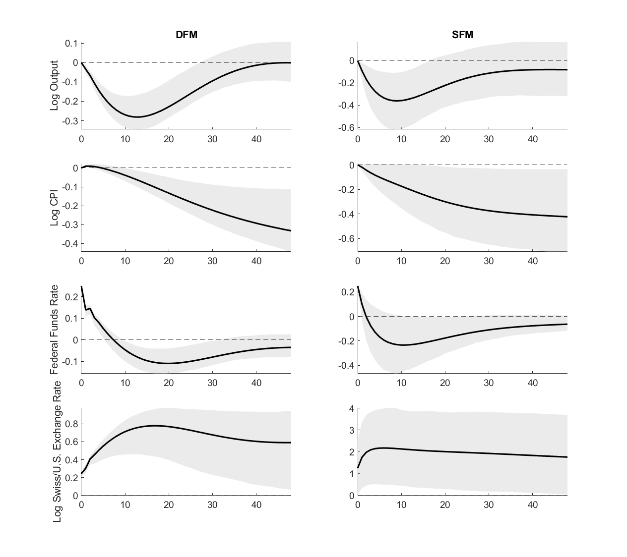
Figure 4 reports impulse responses of log output, log inflation, the federal funds rate, and the log exchange rate. Confidence bands are constructed using a residual bootstrap at the 90% level. The point estimates are qualitatively similar across the two methods. However, confidence bands based on the dynamic factor model (left) are narrower, indicating efficiency gains from direct estimation of dynamic factors.
References↩︎
Department of Economics, Indiana University (Email: ha1@iu.edu). I am grateful to Joon Y. Park, Yoosoon Chang, Keli Xu, and Laura Liu for excellent advice and suggestions. I also thank the participants of the 2023 MEG Meeting, especially Bin Chen, who gave numerous useful suggestions, and the participants of 2024 SETA. All errors are my own.↩︎
The dynamic factor model studied in this paper allows the factor process \((f_t)\) is allowed to exhibit arbitrary serial dynamics, provided that it satisfies the Assumption 1 to be introduced in Section 2. This is in contrast to the generalized dynamic factor model of [5].↩︎
The associated number of dynamic factors were found to be four, which increases to seven after the onset of COVID.↩︎
Assumption 1 is discuss in more detail in the Supplemental Materials 9.3.↩︎
[3] mentions but does not pursue the possibility of extending their theory to infinite-order VAR processes with rapidly decaying coefficients.↩︎
Derivation of the discrete Fourier transform needed to solve the first order condition is given in the Supplemental Materials 9.4.↩︎
In both [3] and [4], we used IC test whenever it was needed to test for the number of static factors. When the lag order of the VAR(\(p\)) model needed to be specified, we used \(p=1\) for the first three specifications and \(p=2\) for the fourth specification. For [3], we used the default parameters \((\delta,m)=(0.1,1)\) with covariance matrix method. For [4], we used the residuals from direct regression, i.e., \(\hat{Y}_t^B\) in [4].↩︎
Additional zero restrictions, other than on contemporaneous response of industrial production and CPI, can be imposed. In that case, the restrictions become over-identifying and must be enforced during estimation. This is straightforward in our alternating least squares framework. For example, in the factor loading update step, one may impose zero restrictions via constrained least squares on \((\hat{f}_t)\).↩︎