Bayesian Predictive Synthesis for Dynamic Networks: Forecasting and Identifying Structural Mechanisms
June 18, 2026
Abstract
Networks are shaped by competing structural mechanisms, such as communities, geometry, or hubs. In a dynamic network the most predictive mechanism can change, and a model tied to one mechanism, or to fixed weights, cannot adapt as the dominant structure shifts. We develop dynamic Bayesian predictive synthesis for networks, in which a mechanism is an agent forecasting the next snapshot’s edges and a synthesis layer combines them with time-varying weights. At each step the method returns a calibrated edge forecast and inference on the mechanism weights, with intervals valid given the fitted agents, so it also reports which mechanism is most informative. Inference of this kind requires a sparse-safe parametrization and an identification theory, under which a single graph identifies and estimates the weights. A sharp threshold separates distinguishable from indistinguishable mechanisms, a change in the active mechanism is tracked at an optimal per-switch cost, and for a single snapshot the method reduces to calibrated link prediction. On real networks, simulations, and benchmarks, the synthesis gives accurate, calibrated forecasts and recovers the leading mechanism when agents are well separated.
Keywords: dynamic networks; Bayesian predictive synthesis; forecast combination; calibration; link prediction.
0.0.1 Introduction↩︎
A network observed at a single time is often modeled as a draw from a generative mechanism. Three families are standard: stochastic block models for community structure [1], [2], latent-position and random dot product graphs for geometry [3], [4], and configuration or Chung–Lu models for degree heterogeneity [5]. Two difficulties arise in practice. First, the practitioner rarely knows which mechanism generated the data. Second, when the network changes over time, the mechanism that best explains it changes as well. Contact networks alternate between community structure during class and hub structure during breaks within a single day, and co-authorship and online social networks reorganize as communities form and dissolve. A model committed to one mechanism cannot follow such a change. Combining several mechanisms with weights set in advance does not help. Once the most predictive mechanism changes, those weights still favor the mechanism that was dominant before, and the combination misrepresents the current structure. We instead let the weights change with the network and estimate them from data. The weights become the object of inference: we estimate them, with uncertainty, from a single network snapshot, and we track their change over time. The weight on an agent is a residualized log-odds projection coefficient: a positive value means that agent carries predictive structure beyond the others, not that the network was generated by that mechanism, so the leading mechanism is a pool-dependent statement and adding or removing an agent can move the lead. Forecast combination for time series learns such weights from a long history.
The changing balance of mechanisms raises three questions. Can the weights on competing mechanisms be learned from data, not fixed in advance? At what rate can they be learned from a single network? And can the resulting forecast be trusted as a calibrated probability? Existing work does not answer them. Forecast combination is developed for time series, not for graph-valued outcomes with single-snapshot inference. Network estimation treats a single fixed graph, not weights that follow a changing mechanism.
We extend dynamic Bayesian predictive synthesis to networks. Predictive synthesis [6], [7] specifies how a set of agent forecasts relates to the outcome, and updates that specification as agents and outcomes are observed. Each mechanism is fit to the history and forecasts the edge probabilities of the next network snapshot. A synthesis layer combines these forecasts on the logit scale through time-varying coefficients. The coefficients are the state of a dynamic linear model [8]: they drift as a random walk and are updated against the observed edges. At each step the method returns two things: a calibrated forecast of the next edges, and an estimate of the weights with its uncertainty. With a single time point, it reduces to calibrated link prediction.
A network on \(n\) nodes has of order \(n^2\) node pairs. Under a conditionally independent edge model, each pair is a Bernoulli observation, and the Fisher information for the weights is of order \(n^2\rho_n\), where \(\rho_n\) is the edge density. The weights are therefore estimable from one network snapshot, at rate \((n^2\rho_n)^{-1/2}\), a rate set by the size of the network, not the length of the series. In a large network \(n^2\rho_n\) is in the thousands even at low density, while a change in the most predictive mechanism takes a few snapshots, so the weights are estimated faster than they change. The same quantity \(n^2\rho_n\) also determines the contrast two mechanisms need to be distinguished from one network snapshot, and the rate at which a change in mechanism is tracked.
Bayesian predictive synthesis grew out of the reconciliation of probability assessments [9], [10] and the modeling of probabilistic agent opinion [6], [11], in which a decision maker updates a prior over an outcome by treating the agents’ predictive distributions as data through a conditional synthesis density. [7] made the synthesis dynamic for time series by letting the synthesis coefficients follow a dynamic linear model, and [12] carried it to multivariate macroeconomic forecasting; [13] developed agent-specific calibration, [14] introduced decision-guided synthesis, and [15] replaced the linear synthesis function with a nonparametric tree ensemble. The construction generalizes Bayesian model averaging [16] and the stacking of predictive distributions [17]–[19], and is related to opinion pools [20] and optimal prediction pools [21]. Every paper in this lineage operates on scalar or vector time series: the outcome is a number or a low-dimensional vector and the agents forecast it. None acts on a graph, where the outcome is an adjacency matrix, the agents are generative network mechanisms, and the unit of information is the dyad. We extend the dynamic synthesis of [7] to networks. Incorporating the network structure into the synthesis yields results with no time-series counterpart: the combination weights are identified and estimated from a single graph, which requires a sparse-safe parametrization and an identification theory the time-series literature does not need.
The work nearest to ours combines several network predictors for one prediction task. [22] stack a large collection of link-prediction algorithms into a near-optimal meta-learner on static networks, [23] extend feature-based stacking to temporal networks, and [24] average latent-space models of differing latent dimension by \(K\)-fold edge cross-validation [25], with asymptotic optimality for link prediction. These are combination methods for networks, and we benchmark against them, but they differ from the present construction in what they return and what they justify: they stack non-mechanistic predictor scores or average models within a single family by a frequentist criterion, so in the convex-pooling form used here they produce a ranking, not a calibrated predictive distribution, carry no calibration intercept, and stay within the convex hull of their inputs, and they provide no inference on the contribution of any mechanism, no single-snapshot identification theory, no separation rate, and no tracking guarantee. [26] combine network mechanisms at the population graphon; they use no dynamic state and give no inference on a finite graph. [27] study, for one fixed graph, when two mechanisms are distinguishable, and [28] model time-varying spillovers on a network in state-space form. The present paper differs in three ways. It estimates the combination weights, with uncertainty, from a finite graph. It tracks a change in the active mechanism at an optimal per-switch cost. And it shows when model averaging fails under misspecification.
The agents instantiate the standard families. The community agent is the stochastic block model [1] in its mixed-membership [29] and spectral [30] forms; the latent-geometry agent is the latent space model [3] and the random dot product and generalized random dot product graphs [4], [31]; the degree agent is the Chung–Lu model [5]; and the local agent is the Adamic–Adar index [32]. We treat each as a one-step-ahead predictive distribution and combine them, not selecting one [33], [34] or merging their parameters into a single hybrid model.
A parallel response to dynamic networks fits a single dynamic generative model: dynamic latent space models [35], [36], dynamic stochastic block models [37], [38], and temporal exponential random graph models [39], [40], surveyed alongside the static families by [41]. Each commits to one mechanism for the entire series. The present method instead holds several mechanisms at once and lets a dynamic synthesis layer reweight them as their relative fit changes, the regime-switching behavior the experiments target.
Two further threads fix the scale of the theory. [42] show that a graph carries between \(O(n)\) and \(O(n^2)\) units of information about a tie propensity according to its density, and the dyadic-inference literature [43], [44] treats the dyad count as the unit of information; we use this to set the rate at which combination weights, not model parameters, are learned from a single snapshot. Detection thresholds for a fixed graph, community recovery at the Kesten–Stigum boundary [45]–[47], latent-geometry detection [48], and global structure tests [49], [50], have as their snapshot-wise, mechanism-against-mechanism analogue our separation rate inside a tracking problem, with graphon estimation rates [51], [52] entering through the agents. Dynamic model averaging [53] tracks which model is active over time but, as an averaging rule, inherits the misspecification collapse [54], [55] that Theorem 4 formalizes and the experiments expose, while the link-prediction problem itself [56], [57] is the \(T=1\) task that our construction calibrates.
We develop dynamic Bayesian predictive synthesis for dynamic networks: each candidate mechanism is used as an agent that forecasts the next snapshot’s edges, and a synthesis layer combines these forecasts with weights that drift over time, so the method is at once a calibrated one-step-ahead edge forecaster, in the Bayesian predictive synthesis tradition of [7], [12] and scored sequentially by a proper scoring rule, and a reading of which mechanism is currently active. A sparse-safe parametrization keeps it valid on sparse graphs, and with a single snapshot it reduces to calibrated link prediction. The main contribution is a theory for these combination weights, built on one fact: a graph on \(n\) nodes at sparsity \(\rho_n\) contains on the order of \(n^2\rho_n\) edges, so the weights are learned from a single snapshot, not from a long series. The theory establishes five properties of these weights. First, the weights are identified and estimable from one snapshot, with a normal limit; their intervals are valid conditional on the fitted agents, and remain valid unconditionally for finite-dimensional mechanisms through a cross-fold orthogonal correction that accounts for refitting the agents on the same graph. Second, two mechanisms are distinguishable from one snapshot precisely when their edge probabilities differ by more than a threshold that no test can improve upon. Third, a change in the active mechanism is tracked at a cost incurred only at the changes, at a rate matching a minimax lower bound. Fourth, when no agent is correct, the weights converge to a well-defined projection, the forecast remains calibrated, and the synthesis improves on Bayesian model averaging, which under misspecification collapses onto one agent. Fifth, the static link-prediction case carries a case-control correction.
We evaluate the method on five real dynamic networks, controlled simulations, and link-prediction benchmarks, comparing against model averaging, stacking, and purpose-built dynamic network models. The real networks are a financial correlation network, high-school and hospital-ward contact networks with known group labels, and two timestamped networks in the tens of thousands of nodes. Two findings stand out. The synthesis produces calibrated forecasts together with interpretable, time-varying weights that carry valid intervals; a recalibrated latent-space competitor matches the probabilities only after a separate recalibration step and returns no weights, so the contribution is calibrated forecasting with mechanism inference.
0.0.2 Dynamic networks and mechanism agents↩︎
We observe a sequence of undirected networks on a fixed node set \(V=\{1,\dots,n\}\), recorded as symmetric adjacency matrices \(A_1,\dots,A_T \in \{0,1\}^{n\times n}\) with zero diagonal. Conditionally on a symmetric edge-probability matrix \(P_t \in [0,1]^{n\times n}\), the upper-triangular entries of \(A_t\) are independent Bernoulli draws, \(A_{t,ij}\sim \mathrm{Bernoulli}(P_{t,ij})\) for \(i<j\). We work in the sparse regime \[\label{eq:sparse} P_t = \rho_n\, M_t, \qquad \rho_n \to 0, \qquad n\rho_n \ge c\log n,\tag{1}\] where \(\rho_n\) is a global sparsity factor and \(M_t\) is a bounded structural matrix; the condition \(n\rho_n\ge c\log n\) keeps the average degree above the connectivity threshold [58].
A mechanism agent is a forecaster that maps the history \(A_{1:t-1}\) to a one-step predictive edge-probability matrix \(\widehat{P}^{(j)}_t\). We use three model-based agents.
SBM (community). A degree-corrected stochastic block model [2] fit by regularized spectral clustering [30], [59], yielding block assignments and Laplace-smoothed block connection probabilities; \(\widehat{P}^{\mathrm{SBM}}_{t,ij}\) is the estimated probability for the blocks of \(i\) and \(j\).
GRDPG (geometry). A generalized random dot product graph fit by adjacency spectral embedding with magnitude-truncated eigenvalues [4]; \(\widehat{P}^{\mathrm{GRDPG}}_{t,ij}= x_i^{\!\top}I_{p,q}\, x_j\) for embedded positions \(x_i\) and signature \((p,q)\).
Chung–Lu (degree). A sparse degree model \(\widehat{P}^{\mathrm{CL}}_{t,ij}= d_i d_j / (2m)\) with degrees \(d_i\) and edge count \(m\) [5], truncated to the sparse scale by the two-sided clip of Section 0.0.3 so that high-degree pairs do not exceed it; this is closely related to the preferential-attachment per-dyad score.
For link prediction we additionally include a local per-dyad agent, Adamic–Adar [32], [56], \(\mathrm{AA}(i,j)=\sum_{z\in N(i)\cap N(j)} 1/\log d_z\), mapped to a probability by the fixed, label-free squashing \(\widehat{P}^{\mathrm{AA}}_{t,ij}=1-e^{-\mathrm{AA}(i,j)/\tau}\), with \(\tau\) the mean Adamic–Adar score over the scored dyads. The three model-based agents are those for which Theorem 1 supplies explicit rates; the local agent is a nonparametric predictor that the oracle inequality covers without a parametric rate.
0.0.3 Dynamic Bayesian predictive synthesis↩︎
Let \(\sigma(\cdot)\) denote the logistic function and \(\mathrm{logit}\) its inverse. Stack the agent predictives for a dyad \((i,j)\) at time \(t\) into a feature vector \(z_{t,ij} = (1,\, \mathrm{logit}\widehat{P}^{(1)}_{t,ij},\dots,\mathrm{logit}\widehat{P}^{(J)}_{t,ij})^{\!\top}\). The synthesis predictive is the affine-logit pool \[\label{eq:synthesis} \widetilde{P}_{t,ij} = \sigma\!\big(\boldsymbol{\beta}_t^{\!\top}z_{t,ij}\big), \qquad \boldsymbol{\beta}_t = (\beta_{t0},\beta_{t1},\dots,\beta_{tJ})^{\!\top}\in \mathbb{R}^{J+1},\tag{2}\] where \(\beta_{t0}\) is a calibration intercept and \(\beta_{tj}\) is the time-\(t\) weight on agent \(j\). Each \(\beta_{tj}\) is a log-odds weight, not a mixture share: a positive value indicates that agent \(j\) aligns with the edge structure left unexplained by the other agents, and a negative value that it is anti-aligned (Table 1). The individual weights are interpretable when the agents are not aliased, a condition made precise in Section 0.0.4.
| Weight pattern | Reading |
|---|---|
| Large positive standardized contribution | agent supplies residual predictive structure beyond the others |
| Near zero | agent is redundant given the others |
| Negative | agent is anti-aligned with the edges, a sign of misspecified or opposite structure |
| Ill-conditioned \(H_t\) (large \(\kappa\)) | individual weights are not separately interpretable |
The coefficient vector is the latent state of a dynamic linear model [8]: \[\label{eq:dlm} \boldsymbol{\beta}_t = \boldsymbol{\beta}_{t-1} + \omega_t, \quad \omega_t \sim \mathcal{N}(\boldsymbol{0}, W_t), \qquad A_{t,ij} \mid \boldsymbol{\beta}_t \sim \mathrm{Bernoulli}\!\big(\sigma(\boldsymbol{\beta}_t^{\!\top}z_{t,ij})\big).\tag{3}\] The evolution variance \(W_t\) is set by a single discount factor \(\delta\in(0,1]\), which controls how quickly weights may move: \(\delta=1\) holds the weights fixed (suited to \(T=1\)), while \(\delta<1\) permits tracking. A single discount controls the whole filter, and the results below are insensitive to its value: sweeping \(\delta\in[0.7,0.95]\) leaves one-step-ahead switch recovery at a single snapshot, the agent-refit lag, up to \(\delta=0.95\), while the transductive recovery time, which carries no refit lag, scales as \(1/(1-\delta)\) exactly as the tracking bound predicts, so a default near \(0.9\) suffices and no per-network tuning of the discount is needed. The Bernoulli observation gives no closed-form update, so we use a Laplace (extended-Kalman) step. The posterior mode is computed by damped Newton iteration with step-halving, which decreases the negative log posterior monotonically, and the curvature at the mode is propagated as the posterior covariance. The one-step forecast is the plug-in predictive \(\sigma(\widehat\boldsymbol{\beta}_{t\mid t-1}^\top z_{t,e})\) at the filtered mean; the curvature enters the weight intervals but not the point forecast. The agents are fit on a fold of dyads held out from the fold used to update the synthesis, so no dyad is used both to fit an agent and to estimate the weights. The forward pass at each time \(t\) is: fit the agents on \(A_{1:t-1}\) and form the features \(z_t\); compute the one-step-ahead forecast \(\widetilde{P}_t\) from the current state; and, on observing \(A_t\), filter \(\boldsymbol{\beta}_t\) by the discounted Bernoulli update.
0.0.3.0.0.1 Sparse-safe parametrization.
In the sparse regime \(\rho_n\to0\) a fixed affine-logit pool of raw logits need not preserve the global density, so for the analysis (and in the implementation) we separate the density from the structural combination. Writing \(\rho_n\) for an estimate of the global edge density (the observed dyad mean), set the centered agent features and the offset synthesis \[\label{eq:offset} u^{(j)}_{t,ij} = \mathrm{logit}\widehat{P}^{(j)}_{t,ij} - \log\rho_n, \qquad \widetilde{P}_{t,ij} = \sigma\!\Big(\log\rho_n + \alpha_t + \textstyle\sum_{j=1}^J \theta_{tj}\, u^{(j)}_{t,ij}\Big),\tag{4}\] so \(\log\rho_n\) is a fixed offset carrying the density, \(\alpha_t\) is the calibration intercept, and \(\theta_t=(\theta_{t1},\dots,\theta_{tJ})\) are the structural weights; the state is \(\boldsymbol{\beta}_t=(\alpha_t,\theta_t)\). The clipping of \(\widehat{P}^{(j)}\) is at the sparse scale on both sides, \([\rho_n\epsilon,\,\rho_n/\epsilon]\) intersected with \([\rho_n\epsilon,\,1-\epsilon]\), not a fixed \([\epsilon,1-\epsilon]\). The two-sided sparse cap keeps the centered features bounded, \(|u^{(j)}_{t,e}|\le\log(1/\epsilon)+O(\rho_n)\), as Assumption 2 and the design condition of Theorem 1 require; without an upper cap at the sparse scale a high-degree Chung–Lu dyad with \(d_id_j/(2m)=O(1)\) would give \(u^{(j)}_{t,e}\asymp\log(1/\rho_n)\to\infty\), so the cap, not merely the lower clip, is what enforces boundedness, and it does not distort the density as \(\rho_n\to0\). In the implementation the density level is carried entirely by the free intercept \(\alpha_t\), which the filter updates from past snapshots only, so the one-step-ahead forecast uses no information from the snapshot being scored; the fixed offset \(\log\rho_n\) of the theory and the filtered intercept differ only by a constant that \(\alpha_t\) absorbs, leaving the structural-weight inference unchanged. The theory states a single scale \(\rho_n\) for transparency; the statements and rates carry over unchanged to a time-varying \(\rho_{t,n}\) with \(c\rho_n\le\rho_{t,n}\le C\rho_n\) uniformly in \(t\), on replacing \(N_t\asymp n^2\rho_n\) by \(N_t\asymp n^2\rho_{t,n}\). The theory below targets the population weight \(\boldsymbol{\beta}^\circ_t\) in this parametrization.
0.0.3.0.0.2 Computation.
The agents are standard static network models fit to the observed history; the dynamic linear model acts only on the low-dimensional vector of weights that combines them, not on the network itself. Because that weight state is Gaussian and linear, its recursion uses standard Kalman filtering and Rauch–Tung–Striebel smoothing [8], [28].
0.0.4 Theory↩︎
Every result in this section is network-specific and is organized around one quantity, the edge information in a single snapshot. With the sparse-safe synthesis 4 , write the dyad feature \(z_{t,e}=(1,u^{(1)}_{t,e},\dots,u^{(J)}_{t,e})^{\!\top}\) for a dyad \(e=(i,j)\) and let \[\label{eq:info} N_t \;:=\; \sum_{e\in\mathcal{E}_t} q_{t,e}(1-q_{t,e}) \;\asymp\; |\mathcal{E}_t|\,\rho_n \;\asymp\; n^2\rho_n , \qquad H_t \;:=\; N_t^{-1}\!\sum_{e\in\mathcal{E}_t} q_{t,e}(1-q_{t,e})\,z_{t,e}z_{t,e}^{\!\top},\tag{5}\] where \(q_{t,e}=q_{t,e}(\boldsymbol{\beta}^\circ_t)\) and \(\mathcal{E}_t\) is the set of sampled dyads. \(N_t\) is the scalar dyadic information scale and grows as the expected edge count of one graph, never as the series length \(T\); \(H_t\) is the normalized information matrix, so \(N_tH_t\) is the Fisher information for the weights. The central object is the population log-odds projection of the network onto the set of mechanisms, \[\label{eq:popbeta} \boldsymbol{\beta}^\circ_t \;=\; \mathop{\mathrm{arg\,min}}_{\boldsymbol{\beta}\in\Theta}\; R_t(\boldsymbol{\beta}), \qquad R_t(\boldsymbol{\beta}) \;=\; \frac{1}{|\mathcal{E}_t|}\sum_{e\in\mathcal{E}_t} \mathrm{KL}\!\big\{\mathrm{Bern}(p_{t,e}),\,\mathrm{Bern}(q_{t,e}(\boldsymbol{\beta}))\big\},\tag{6}\] and the theory is about estimating, tracking, calibrating, and interpreting \(\boldsymbol{\beta}^\circ_t\). Three results are the headline. First, a single snapshot identifies and estimates the weights at the dyadic-information rate, with an aliasing condition for when individual weights are recoverable (Theorem 1); this single-graph identification has no time-series counterpart and is the conceptual core. Second, two mechanisms separate above a contrast threshold, and a switch in the active mechanism is tracked with a bounded recovery delay that is minimax-optimal up to constants (Theorems 2 and 3, with the matching lower bound in Section 0.0.13 of the Supplement). Third, when no agent equals the truth the weights converge to a log-odds projection and the intercept enforces calibration, separating the synthesis from model averaging and stacking under misspecification in this setting (Theorem 4). A corollary specializes the first result to one snapshot, recovering calibrated link prediction (Corollary 1).
We write \(a_{n,t}\) for the agents’ estimation error on the information-weighted logit (score) scale, \(a_{n,t}^2=N_t^{-1}\sum_e q_{t,e}(1-q_{t,e})\,|\widehat z_{t,e}-z^\circ_{t,e}|^2\), the deviation of the fitted dyad logits from their population targets; the probability-scale graphon rates cited in Assumption 2 convert to this scale through the sparse lower bound \(p_{t,e}\asymp\rho_n\), which amplifies probability error by \(1/\rho_n\) (Supplement S2), and \(r_{\mathrm{Lap}}\) for the Laplace/extended-Kalman linearization error of the filter.
Assumption 1 (Sparsity). The edge probabilities satisfy 1 with the entries of \(M_t\) bounded in \([c_0,C_0]\) on their support scale, and the average degree exceeds the connectivity threshold, \(n\rho_n\ge c\log n\). The number of blocks \(K\) and the embedding dimension \(d=p+q\) are fixed.
Assumption 2 (Agent regularity and rates). After two-sided sparse-scale clipping to \([\rho_n\epsilon,\,\rho_n/\epsilon]\cap[\rho_n\epsilon,\,1-\epsilon]\), each centered agent feature \(u^{(j)}_{t,e}\) is bounded, \(|u^{(j)}_{t,e}|\le\log(1/\epsilon)+O(\rho_n)\); the upper sparse cap is what enforces this, since a Chung–Lu hub with \(\widehat{P}^{(j)}_{t,e}=O(1)\) would otherwise give \(u^{(j)}_{t,e}\asymp\log(1/\rho_n)\). The model-based agents are consistent for their best-fitting parameters. On the probability scale the dyadic mean-squared error of the fitted edge probabilities is of order \(\rho_n(K^2/n^2+\log K/n)\) (SBM, [51], [59]), \(\rho_n d/n\cdot\mathrm{polylog}\,n\) (GRDPG, [4], [58]), and \(\rho_n/n\) (Chung–Lu). Because a centered logit feature equals the relative probability deviation, the score-scale quantity \(a_{n,t}^2\) defined above is larger by \(\rho_n^{-2}\): thus \(a_{n,t}^2\asymp K^2/(n^2\rho_n)\) (SBM, the \(\log K/n\) clustering term a loose worst-case bound that does not bind for fixed separated blocks), \(d/(n\rho_n)\cdot\mathrm{polylog}\,n\) (GRDPG), and \(1/(n\rho_n)\) (Chung–Lu).
Assumption 3 (Design non-degeneracy). The normalized information matrix is well conditioned, \(\lambda_{\min}(H_t)\ge \underline\lambda>0\) uniformly in \(t\). This is a quantitative strengthening of the condition that the agents’ dyad-logit surfaces \((1,u^{(1)}_{t,e},\dots,u^{(J)}_{t,e})\) are not affinely dependent across dyads, and is the identifiability condition for \(\boldsymbol{\beta}^\circ_t\); its failure is the aliasing of Theorem 1.
Assumption 4 (State evolution). The state \(\boldsymbol{\beta}_t=(\alpha_t,\theta_t)\) follows 3 with discount \(\delta\) and evolution scale \(\tau^2=1-\delta\). A comparator sequence \(\boldsymbol{\beta}^\circ_t\) has total movement \(\sum_{t=2}^T\|\boldsymbol{\beta}^\circ_t-\boldsymbol{\beta}^\circ_{t-1}\|^2\le \mathcal{V}\), realized by \(S\) regime switches of jump size at most \(D\) in the piecewise-stable case.
0.0.4.1 Single-snapshot dyadic-rate identification and aliasing
One result separates network synthesis from time-series synthesis. A single graph identifies and estimates the weights, at a rate set by the size of the graph, not the length of the series. The one-snapshot estimator \(\widehat\boldsymbol{\beta}_t\) is the cross-fitted maximum a posteriori (or, with a flat prior, maximum likelihood) logistic fit of the dyads \(A_{t,e}\) on the offset design \(z_{t,e}\).
Theorem 1 (Single-snapshot identification, dyadic rate, and aliasing). Fix \(t\), condition on the sigma-field \(\mathcal{F}_{t,n}\) generated by the history, the cross-fitted agents, the sampled dyad set \(\mathcal{E}_t\) (with \(m_{t,n}=|\mathcal{E}_t|\)), the offset \(\log\rho_n\), and the true conditional edge probabilities \(p_{t,e}\), and assume the dyad set is conditionally non-informative, so that \(A_{t,e}\sim\mathrm{Bernoulli}(p_{t,e})\) are independent given \(\mathcal{F}_{t,n}\). Suppose the basic sparse-scale conditions hold: the parameter space \(\Theta\) is compact and convex, \(\max_e\|z_{t,e}\|\le B\), and there are constants \(0<c_q<C_q\) with \(c_q\rho_n\le q_{t,e}(\beta)\le C_q\rho_n\le\tfrac12\) uniformly on \(\Theta\), \(p_{t,e}\le C_p\rho_n\), and \(m_{t,n}\rho_n\to\infty\) (Supplement S1, conditions B1–B3).
(Identification and aliasing.) Because \(q_{t,e}(1-q_{t,e})>0\), the null space of \(H_t(\beta)\) equals \(\mathcal{N}_t=\{a:a^{\!\top}z_{t,e}=0\;\forall e\in\mathcal{E}_t\}\) for every \(\beta\). Hence the conditional synthesis law \(\beta\mapsto\{q_{t,e}(\beta)\}\) is identified if and only if \(H_t\) is full rank (\(\mathcal{N}_t=\{0\}\)); otherwise \(\beta\) is identified only modulo \(\mathcal{N}_t\), and a linear functional \(a^{\!\top}\beta\) is estimable iff \(a\in\mathrm{Range}(H_t)\). An exact affine dependence among \(1,u^{(1)}_{t,\cdot},\dots, u^{(J)}_{t,\cdot}\) aliases the corresponding separate agent weights.
(Rate and conditional normality.) Adding interior, Gram-nonsingularity, and weak-penalty conditions (Supplement S1, C1–C4), the one-snapshot estimator \(\widehat\boldsymbol{\beta}_t\) satisfies, conditionally on \(\mathcal{F}_{t,n}\), \[\label{eq:t1rate} \|\widehat\boldsymbol{\beta}_t-\boldsymbol{\beta}^\circ_t\| = O_p\!\Big(\sqrt{\tfrac{J+1}{N_t}}\Big), \quad N_t\asymp m_{t,n}\rho_n\asymp n^2\rho_n \;(\text{with } m_{t,n}\asymp n^2 \text{ for full-snapshot synthesis}),\tag{7}\] with the asymptotic linear representation \(\sqrt{N_t}(\widehat\boldsymbol{\beta}_t-\boldsymbol{\beta}^\circ_t)= H_t^{-1}N_t^{-1/2}\sum_e(A_{t,e}-p_{t,e})z_{t,e}+o_p(1)\) and therefore \[\label{eq:t1clt} \sqrt{N_t}\,\big(\widehat\boldsymbol{\beta}_t-\boldsymbol{\beta}^\circ_t\big) \;\Rightarrow\; \mathcal{N}\!\big(0,\;H_t^{-1}V_t H_t^{-1}\big), \quad V_t=H_t \text{ under correct Bernoulli-logit specification.}\tag{8}\] The effective sample size is the edge count: every weight is estimable from one graph at the dyadic rate \((n^2\rho_n)^{-1/2}\), not the series rate. If the fitted-agent population score is within \(O_p(a_{n,t})\) of an oracle score and the implemented filter is within \(O_p(r_{\mathrm{Lap}})\) of \(\widehat\boldsymbol{\beta}_t\), then the oracle-centered error is \(O_p(\sqrt{(J+1)/N_t}+a_{n,t}+r_{\mathrm{Lap}})\), and the oracle-centered limit holds with the same covariance when \(\sqrt{N_t}\{a_{n,t}+r_{\mathrm{Lap}}\}\to0\).
The Fisher information for the weights is of order \(n^2\rho_n\), so they are estimable from a single network, without a time series. The case \(T=1\), a single network on a fixed node set, is the static link-prediction specialization of the same estimator. The rank condition in Assumption 3 is a diagnostic of identifiability: when it fails, two mechanisms are aliased and their individual weights are not separately identified.
The limit of Theorem 1 is conditional on the fitted agents. When a flexible agent is refit on the same snapshot, the conditional intervals can undercover. The following debiased construction removes the bias. Split the synthesis dyads of snapshot \(t\) into \(K\) folds \(I_1,\dots,I_K\), estimate each agent surface on the dyads outside a fold, and replace the synthesis score \(s_e(\boldsymbol{\beta},\xi)=z_e(\xi)\{A_e-q_e(\boldsymbol{\beta},\xi)\}\) by a fold-specific orthogonal score \(\psi^\perp_{k,e}=s_e-c_{k,e}\), where the correction \(c_{k,e}\) is built from the nuisance influence function so that it annihilates the first-order effect of agent-estimation error, \(\partial_\xi\Psi^\perp_{n,k}(\boldsymbol{\beta}^\circ,\xi^\circ)[h]=0\), while preserving the projection target \(\boldsymbol{\beta}^\circ\). Let \(\widetilde{\boldsymbol{\beta}}\) solve the cross-fold orthogonal estimating equation \(\sum_{k}\sum_{e\in I_k}\psi^\perp_{k,e}(\boldsymbol{\beta},\widehat\xi^{-k})=0\), with \(\widehat\xi^{-k}\) measurable with respect to the out-of-fold data.
The synthesis is computed in two passes. The filtering pass of 3 produces the one-step-ahead forecast and the weight point estimates. The cross-fold orthogonal pass produces weight estimates whose confidence intervals remain valid when the agents are refit on the same graph. The forecasts below use the first pass; the weight intervals use the second.
This unconditional validity is the content of the cross-fold orthogonal limit. The orthogonal estimator is asymptotically normal unconditionally over the dyad draw, the random fold split, and the agent refits under a score-scale agent-error rate of \(o(N_t^{-1/4})\), far weaker than the \(o(N_t^{-1/2})\) the conditional limit needs. This second-order rate is met by agents whose parameter count is fixed, so that each parameter is informed by order \(n^2\) dyads: the SBM block probabilities give \(a_{n,t}^2\asymp K^2/(n^2\rho_n)\), hence \(\sqrt{N_t}\,a_{n,t}^2\asymp K^2/(n\sqrt{\rho_n})\to0\). It is not met in the sparse regime by agents whose \(\Theta(n)\) latent parameters are each informed by only \(\Theta(n)\) dyads: the GRDPG positions and Chung–Lu degrees give \(a_{n,t}^2\asymp d/(n\rho_n)\) and \(1/(n\rho_n)\), so \(\sqrt{N_t}\,a_{n,t}^2\asymp d/\sqrt{\rho_n}\) and \(1/\sqrt{\rho_n}\) do not vanish. The unconditional Wald intervals are therefore established for the finite-dimensional community weight; for every agent the conditional limit of Theorem 1, centered at the fitted projection, supplies valid intervals given the fitted features. The construction is dyadic double/debiased machine learning [44] specialized to a structure those methods do not address: the nuisances are network models refit on the same graph on which the weights are estimated, and the target is the vector of interpretable mechanism weights.
0.0.4.2 A separation rate for distinguishing mechanisms
The scale \(n^2\rho_n\) also determines how far apart two mechanisms must be to be distinguished from a single network snapshot. The natural object is a separation rate in graphon log-odds, not a density threshold; a hard \(n^2\rho_n=O(1)\) regime is excluded by Assumption 1 (which forces \(n^2\rho_n\ge cn\log n\to \infty\)), so the boundary lives at vanishing contrast inside the assumed regime.
The argument rests on a perturbation lemma for sparse Bernoulli-logit models: on the sparse scale, the divergence between two edge laws is controlled by the dyadic log-odds gap.
Lemma 1 (Sparse Bernoulli-logit perturbations). Let \(p,q\in(0,1)\) with \(x=\mathrm{logit}q-\mathrm{logit}p\), and suppose \(c_0\rho\le p,q\le C_0\rho\le\tfrac12\) and \(|x|\le\eta_0\) for fixed constants. Then there are \(0<c<C<\infty\), depending only on \(c_0,C_0,\eta_0\), such that the Kullback–Leibler divergence, the negative log Hellinger affinity, and the chi-square divergence between \(\mathrm{Bern}(q)\) and \(\mathrm{Bern}(p)\) are all between \(c\,p(1-p)x^2\) and \(C\,p(1-p)x^2\) (the chi-square only bounded above), with the same bounds when \(p,q\) are interchanged; and the per-dyad log-likelihood-ratio has variance at most \(C\,p(1-p)x^2\).
Theorem 2 (Mechanism separation rate and tracking). Let two mechanism configurations produce sparse edge laws \(p_e,q_e\asymp\rho_n\) over \(m_{t,n}\asymp n^2\) conditionally independent dyads, with bounded dyadic log-odds gap \(x_e=\mathrm{logit}q_e-\mathrm{logit}p_e\), and aggregate Fisher signal \(S_n=\sum_e p_e(1-p_e)x_e^2\asymp n^2\rho_n\Delta_n^2\) under a uniform gap \(|x_e|\asymp\Delta_n\). Let the synthesis track with discount \(\delta\).
(Achievability and tracking.) If \(S_n\to\infty\) (equivalently \(n^2\rho_n\Delta_n^2\to\infty\)), the likelihood-ratio test separates the two configurations from a single snapshot with total error tending to zero, and between switches the filtered synthesis recovers the active weight at the per-snapshot squared rate \(O((n^2\rho_n)^{-1})\), the drift over the horizon contributing the discounted tracking regret \(O(\bar N\,\mathcal{V}/(1-\delta)^2)\) of Theorem 3.
(Impossibility.) If \(S_n=O(1)\) (equivalently \(n^2\rho_n\Delta_n^2=O(1)\)), the two snapshot laws are mutually contiguous and no test, hence no measurable functional of the data, separates them consistently: no test has power tending to one, and the minimax total testing error is bounded below by a positive constant; in the limiting case \(S_n\to0\) the power of every test tends to its size.
The critical separation rate is therefore \(\Delta_n\asymp(n^2\rho_n)^{-1/2}\): two mechanisms are distinguishable from one snapshot precisely when their graphon log-odds differ by more than \((n^2\rho_n)^{-1/2}\), and affinely dependent mechanisms (\(\Delta_n=0\)) are never distinguishable at any density.
Remark 1 (Temporal tracking versus single-graph distinguishability). Theorem 2 concerns tracking a moving target and is distinct from asking whether two mechanisms can be distinguished in one fixed graph, the static question studied by [27]. The two boundaries share the scale \(n^2\rho_n\) for the same elementary reason, that a snapshot’s order-\(n^2\) dyads carry Fisher information of order \(n^2\rho_n\), but the operative quantity here is the discounted accumulated separation \(n^2\rho_n\,\Delta_n^2\,(1-\delta^h)/(1-\delta)\) over an \(h\)-snapshot window, which over the \(O(1)\) snapshots that localization takes reduces to \(\asymp h\,n^2\rho_n\Delta_n^2\) (the \(1/(1-\delta)\) canceling, in agreement with the local rate of Theorem 3) and tends to \(n^2\rho_n\Delta_n^2/(1-\delta)\) in a stable regime; this discount interaction has no counterpart in the static problem.
0.0.4.3 Dynamic tracking, switch recovery, and mechanism localization
Because the weights are learned per snapshot, the filter tracks a switching mechanism by paying only for the switches, and, when the margin condition holds, it identifies the active mechanism once the discounted information exceeds the margin between mechanisms. The following theorem establishes the bounded recovery delay and the margin condition under which the active mechanism is identified, and is tested by the weight-trajectory experiments of Section 0.0.5.
Theorem 3 (Prequential tracking, switch recovery, and localization). Let \(\widehat\boldsymbol{\beta}_{t\mid t-1}\) be the one-step-ahead filtered state. Under Assumptions 1–4 with cross-fitting, \[\label{eq:regret} \begin{align} \sum_{t=1}^{T} |\mathcal{E}_t|\big\{R_t(\widehat\boldsymbol{\beta}_{t\mid t-1})-R_t(\boldsymbol{\beta}^\circ_t)\big\} \;\le\; C\Big[&(J{+}1)\,\lambda_T\big(1+\log T+T(1-\delta)\big)\\ &+ \frac{\bar N}{(1-\delta)^2}\!\sum_{t=2}^T\|\boldsymbol{\beta}^\circ_t-\boldsymbol{\beta}^\circ_{t-1}\|^2 + \bar N\!\sum_{t=1}^T \varepsilon_t^2\Big], \end{align}\tag{9}\] where \(\lambda_T=\log(2(J{+}1)T/\alpha)\), \(\bar N\asymp N_t\asymp n^2\rho_n\) is the per-snapshot information, and the implementation error obeys \(\varepsilon_t\le a_{n,t}+r_{\mathrm{Lap}}\). The left side is the cumulative excess one-step log-loss: \(|\mathcal{E}_t|\{R_t(\cdot)-R_t(\boldsymbol{\beta}^\circ_t)\}\) is the excess expected log-loss of snapshot \(t\) in the per-dyad normalization of 6 . For piecewise-stable comparators with \(S\) switches of size at most \(D\) the movement is \(\sum_{t}\|\boldsymbol{\beta}^\circ_t-\boldsymbol{\beta}^\circ_{t-1}\|^2\le SD^2\), so its contribution is at most \(C\bar N SD^2/(1-\delta)^2\): the synthesis charges for switches, not for every time point. The discounted-filter estimation term \((J{+}1)\lambda_T(1+\log T+T(1-\delta))\) and the agent-and-linearization floor \(\bar N\sum_t\varepsilon_t^2\) are lower order when the agents are well estimated and the Laplace step is accurate. Suppose an active mechanism \(r_t\in\{\mathrm{SBM},\mathrm{GRDPG},\mathrm{CL},\mathrm{AA}\}\) has margin \(\theta^\circ_{t,r_t}-\max_{j\ne r_t}\theta^\circ_{t,j}\ge\kappa>0\), and let \(N_t^\delta=\sum_{s\le t}\delta^{t-s}N_s\) be the discounted effective information. Then \[\label{eq:localize} \|\widehat\boldsymbol{\beta}_{t\mid t}-\boldsymbol{\beta}^\circ_t\|_\infty = O_p\!\Big(\sqrt{\tfrac{\log(JT)}{N_t^\delta}} + \frac{\sum_{s\le t}\delta^{t-s}N_s \|\boldsymbol{\beta}^\circ_s-\boldsymbol{\beta}^\circ_t\|}{N_t^\delta} + a_{n,t}+r_{\mathrm{Lap}}\Big),\tag{10}\] and whenever the right side is below \(\kappa/2\), \(\mathbb{P}\{\mathop{\mathrm{arg\,max}}_j\widehat\theta_{t,j}=r_t\} \to1\). Localization is defined in coefficient space: the agent features \(u^{(j)}_{t,e}\) share the centered-logit scale and are bounded in the same range, so the margin compares commensurable quantities; for a scale-invariant statement one may compare the signed standardized contributions \(\theta_{t,j}\,H_{t,jj}^{1/2}\), to which the same margin argument applies. After a switch the recovery delay is of order \(h=O\big(\log(JT/\alpha)/(N\kappa^2)\;\vee\;\log(D/\kappa)/|\log\delta|\big)\).
Remark 2 (Model averaging has switch inertia). Bayesian model averaging weights by cumulative marginal likelihood, so after a regime of length \(L\) its log-odds for the old mechanism are of order \(L\) and it needs an \(\Omega(L)\)-long window to switch; the discounted filter forgets in \(O(1/(1-\delta))\) steps, independent of \(L\). The wrong-mechanism window of averaging grows with how long the previous mechanism was dominant, whereas the synthesis’s recovery delay does not.
Theorem 3 is an upper bound: the discounted filter localizes the active mechanism within \(O(\log(JT/\alpha)/(N_t^\delta\kappa^2))\) post-switch snapshots and pays \(O(SD^2)\) for \(S\) switches. A matching local minimax lower bound, stated and proved in Section 0.0.13 of the Supplement, shows these rates are minimax-optimal up to constants, not merely attained: on the one-switch sparse family over a uniformly non-aliased design, no procedure, even one told the switch time, the agent arrays, the information level \(N\), and the margin \(\kappa\), localizes the post-switch mechanism in fewer than \(\log J/(n^2\rho_n\kappa^2)\) snapshots, any \(\alpha\)-reliable declaration has expected delay at least \(c\,\log(eJ/\alpha)/(n^2\rho_n\kappa^2)\), and the cumulative reliable delay and switch regret obey matching \(S\log(eJ/\alpha)/(n^2\rho_n\kappa^2)\) and \(S\log J\) floors. The lower-bound constant comes from a two-point/Fano reduction and the upper-bound constant from a Freedman inequality, so the matching is in rate, not in constant.
For \(\delta\) bounded away from \(1\), the discount affects only the constant, since the discounted post-switch information \(N(1-\delta^h)/(1-\delta)\asymp hN\) coincides with the undiscounted \(hN\) over the \(O(1)\) snapshots localization takes, so no \(1/(1-\delta)\) factor enters the rate.
0.0.4.4 Universal misspecification: projection, calibration, and competitor gaps
When no agent equals the truth, the weights converge to a log-odds projection, the intercept enforces calibration through a score equation, and the synthesis improves on model averaging by a computable gap.
Theorem 4 (Projection, calibration, and BMA/stacking gaps). Suppose no agent equals the truth.
(Projection and sparse limit.) The one-snapshot weight converges at \((n^2\rho_n)^{-1/2}\) to \(\boldsymbol{\beta}^\circ_t\), the log-odds projection 6 of the true mechanism onto the set of agents. In the sparse graphon limit \(\rho_n^{-1}\widehat{P}^{(j)}_t\to W^{(j)}_t\) and \(\rho_n^{-1}p_t\to W^\circ_t\), the offset synthesis tends to the log-linear form \(\rho_n^{-1}q_t(\boldsymbol{\beta})\to e^{\alpha_t}\prod_j(W^{(j)}_t)^{\theta_{tj}}=:W_t(\boldsymbol{\beta})\), and \(\boldsymbol{\beta}^\circ_t\) solves the Bernoulli/KL (Poisson-type) variational problem \(\mathop{\mathrm{arg\,min}}_{\boldsymbol{\beta}}\int[W_t(\boldsymbol{\beta})-W^\circ_t\log W_t(\boldsymbol{\beta})]\), not an \(L^2\) projection.
(Calibration.) The score equations \(\sum_e(p_{t,e}-q^\circ_{t,e})=0\) and \(\sum_e(p_{t,e}-q^\circ_{t,e})u^{(j)}_{t,e}=0\) hold: the intercept forces zero average miscalibration and the slopes make the residual orthogonal to the mechanism features. Full reliability additionally requires the approximation error of the set \(\inf_{\boldsymbol{\beta}}\|p_t-q_t(\boldsymbol{\beta})\|_{2,t}\) to be small; the finite-sample bound is \(\mathrm{ECE}_b(\widehat q_t)\le C[\inf_{\boldsymbol{\beta}}\|p_t-q_t(\boldsymbol{\beta})\|_{2,t}+\rho_n(\sqrt{(J{+}1)/N_t} +\sqrt{b/N_t}+a_{n,t}+r_{\mathrm{Lap}})]\), where \(b\) is the number of equal-mass calibration bins (distinct from the block count \(K\)); the estimation, binning, and agent terms enter on the sparse probability scale, hence the factor \(\rho_n\).
(Competitor gaps.) Against Bayesian model averaging, which collapses onto the single Kullback–Leibler-closest agent (or, under ties, the Kullback–Leibler-minimizing set) [54], with \(e_j\) the coefficient vector \((\alpha_t,\theta_t)=(0,\mathbf{1}_j)\) for which the offset gives \(q_t(e_j)=\widehat{P}^{(j)}_t\) exactly, \[\label{eq:gap} R_t(\mathrm{BMA})-R_t(\mathrm{BPS}) \;\to\; \min_j R_t(e_j)-\inf_{\boldsymbol{\beta}\in\Theta}R_t(\boldsymbol{\beta}) \;\ge\;0,\tag{11}\] strict whenever the affine-logit projection strictly improves on every single agent (a Kullback–Leibler/Bregman Pythagorean relation for the affine-natural-parameter family of (a) at an interior projection, and a convexity inequality at the boundary). Against convex stacking we claim no universal dominance, the families differ; but when the truth lies at curvature-distance \(d_t\) outside the convex probability hull of the agents and the affine-logit approximation error \(\epsilon_t\) is at most \(\tfrac12 c\,d_t^2\), the projection improves on convex stacking, \(\inf_{w\in\Delta_J}R_t(\sum_j w_j\widehat{P}^{(j)}_t)-\inf_{\boldsymbol{\beta}} R_t(\boldsymbol{\beta})\ge \tfrac12 c\,d_t^2\).
Remark 3 (What the calibration guarantee gives). Theorem 4(b) gives average calibration, through the intercept score equation, and orthogonality of the residual to the agent features, through the slope equations; the empirical calibration error on held-out dyads is bounded by these plus the approximation error of the set of agents, and after a case-control evaluation the same offset returns population calibration (Corollary 1). None of these is full per-bin reliability, which requires \(\inf_{\boldsymbol{\beta}}\|p_t-q_t(\boldsymbol{\beta})\|_{2,t}\) to be small and is not guaranteed for a fixed set of agents.
0.0.4.5 Static link prediction: case-control correction and graceful failure
The \(T=1\) specialization is static link prediction. Two network-specific points make it precise: the held-out evaluation is a case-control sample, and agents that carry no signal fail gracefully.
Corollary 1 (\(T=1\) oracle, case-control offset, graceful failure). For \(T=1\) with train/validation/test dyad splits and cross-fitted agents, the test risk obeys the oracle inequality \(R_{\mathrm{test}}(\widehat q_{\mathrm{BPS}})\le \inf_{\theta\in\Theta}R_{\mathrm{test}}(q_\theta)+O_p(\sqrt{(J{+}1)/m_{\mathrm{val}}}+a_n)\), and adding an agent cannot raise the oracle risk, strictly lowering it when the new agent carries residual log-score information beyond the existing span. If sampling depends only on the label, \(S\perp X\mid Y\), with positives sampled with probability \(s_1\) and negatives with \(s_0\) (an equal-size negative set is the case \(s_1\gg s_0\)), then \(\mathrm{logit}\mathbb{P}(Y{=}1\mid X,S{=}1)=\mathrm{logit}\mathbb{P}(Y{=}1\mid X)+\log(s_1/s_0)\), so the population-calibrated forecast is \(\widehat p_{\mathrm{pop}}=\sigma(\mathrm{logit}\widehat p_{\mathrm{cc}}-\log(s_1/s_0))\); the intercept \(\alpha\) absorbs this constant, so the synthesis is automatically calibrated to the evaluation sample and a single offset recovers the population scale. Finally, if the agent features carry no ranking signal, \(Y\perp z\), then \(\theta^\circ=0\) and the synthesis reduces to an intercept-only base-rate forecast: no score ranks the dyads better than chance while the expected calibration error tends to zero.
Remark 4 (Identifiability of the predictive; why stacking can out-rank but mis-calibrate). The synthesis acts on edge probabilities, invariant to the SBM permutation and the GRDPG \(O(p,q)\) symmetry, so the predictive and (under Assumption 3) the weight \(\boldsymbol{\beta}^\circ_t\) are identified even when agent parameters are not. Theorem 4(b) decouples ranking from calibration: the ordering of dyads is invariant to the intercept, while calibration is not. A convex combination, which carries no free intercept, can therefore rank well yet remain miscalibrated.
0.0.4.6 Estimation defaults
The procedure below summarizes the estimation: on each snapshot the agents are fit on held-out dyad folds, their forecasts are mapped to centered-logit features, the discounted Laplace filter updates the mechanism weights, and the cross-fold construction returns their intervals. Table 2 lists the defaults used throughout, each paired with the diagnostic that signals when it should be revisited.
| Quantity | Default | Revisit when |
|---|---|---|
| Discount \(\delta\) | \(0.9\) | switches are slower or faster than the \(1/(1-\delta)\) window |
| Logit clip \(\epsilon\) | \(10^{-3}\) | many agent probabilities pile at \(0\) or \(1\) |
| Dyad folds \(K\) | \(5\) | the held-out fold is too small to fit the agents |
| Validation dyads | \(20\%\) held out | the calibration intercept is unstable across folds |
| Weight interpretability | \(\kappa(H_t)\) moderate | \(\kappa(H_t)\) large: report the forecast, not the split of credit |
| Localization | margin \(\kappa\) comfortable | small margin: name no leader; the forecast stays calibrated |
0.0.5 Numerical studies↩︎
We report results on five real dynamic networks in the main text (an S&P 500 correlation network, SocioPatterns high-school and hospital-ward contact networks, and the arXiv HEP-PH and Enron networks at scale) and a sixth, the Bitcoin-OTC trust network, in the Supplement, together with controlled switching simulations. The forecast is evaluated by negative log-likelihood (NLL) and two calibration diagnostics: the Kolmogorov–Smirnov distance of the randomized probability integral transform to uniformity (PIT-KS) and the expected calibration error (ECE). The bootstrap intervals below are descriptive summaries. The competitors are Bayesian model averaging, convex stacking, equal-weight pooling, and each single agent. We report, at each snapshot, the leading structural agent, the one with the largest standardized contribution \(|\theta_{t,j}|H_{t,jj}^{1/2}\); this magnitude is the largest residual predictive contribution, while the signed margin of Theorem 3 controls localization of a positively aligned mechanism. A positive weight means an agent carries predictive structure beyond the others, not that the network was generated by that mechanism, and individual weights are separately interpretable only when the information matrix is well conditioned, its condition number \(\kappa(H_t)\) reported as the aliasing diagnostic (Section 0.0.5.3.0.7).
The studies follow the paper’s results: a financial correlation network for calibration, regime tracking, and localization (Section 0.0.5.1.0.1); two label-carrying contact networks for weight validation (Section 0.0.5.2); controlled simulations that test the single-snapshot theory under known truth (Section 0.0.5.3, Theorems 1–4); and two networks in the tens of thousands of nodes for scale and out-of-sample behavior (Section 0.0.5.4).
Two points frame the comparison. First, the synthesis is evaluated as a calibrated density forecaster that also returns mechanism inference; where a competitor can be recalibrated to match its forecast scores (Section [sec:recalib]), the distinguishing output is the calibrated probabilities delivered jointly with interpretable, uncertainty-quantified mechanism weights in a single pass, not a higher raw score. Second, the time-varying weights do not lower the average forecast score on a stable panel, as the \(\delta=1\) ablation of Section [sec:recalib] shows; their role is switch recovery and mechanism localization, together with the pooling of recent snapshots that sharpens the weights where a single snapshot is too sparse.
0.0.5.1 Dynamic networks: tracking and localization
0.0.5.1.0.1 A financial network from S&P 500 returns.
Asset-return correlation networks change their dominant structure across market regimes. In calm markets, returns cluster by sector, a community structure. In stress, a single market factor dominates and most pairs move together, a low-rank structure. We construct a binary dynamic network from these correlations. From daily closing prices of the \(n=470\) S&P 500 constituents with full history from February 2013 to February 2018, we form log-returns and take non-overlapping quarterly windows. In each window we compute the cross-correlation matrix and threshold \(|\mathrm{corr}|>0.5\) to a binary graph, giving \(T=19\) snapshots on the complete-case panel of constituents with full price histories.
The density of the thresholded graph varies widely, from \(0.018\) with \(1{,}986\) edges in the 2017 calm market to \(0.50\) with \(55{,}214\) edges in the 2015–16 stress episode. The per-snapshot information \(n^2\rho_n\) therefore ranges over a factor of twenty-eight within one dataset. The dense stress snapshots, with density up to \(0.50\), sit outside the sparse regime \(\rho_n\to0\) of 1 ; the sparse-regime guarantees therefore attach to the sparse calm snapshots, while the dense snapshots are a robustness check that the regime tracking persists beyond the theory’s sparsity range. We take the regime label from the data, as the share of the leading eigenvalue of the correlation matrix, which is high in stress and low in calm; this recovers the documented market history from the correlation threshold alone, with no fitting to the volatility series.
| Method | NLL | PIT-KS | ECE |
|---|---|---|---|
| S&P 500 correlation (\(n=470\), \(T=19\)) | |||
| Dynamic BPS | 0.653 | 0.092 | 0.123 |
| Dynamic SBM (smoothed) | 0.829 | 0.245 | 0.284 |
| Dynamic GRDPG (smoothed) | 0.860 | 0.174 | 0.225 |
| BMA | 1.047 | 0.249 | 0.303 |
| DMA (forgetting) | 1.047 | 0.249 | 0.303 |
| Stacking | 0.940 | 0.222 | 0.284 |
| Equal weight | 0.947 | 0.215 | 0.281 |
| SBM agent | 1.053 | 0.251 | 0.305 |
| GRDPG agent | 1.959 | 0.199 | 0.269 |
| Chung–Lu agent | 1.332 | 0.241 | 0.309 |
| High-school contact (\(n=327\), \(T=41\)) | |||
| Dynamic BPS | 0.613 | 0.107 | 0.140 |
| BMA | 2.065 | 0.390 | 0.453 |
| Stacking | 2.015 | 0.394 | 0.454 |
| Equal weight | 2.110 | 0.397 | 0.456 |
| SBM agent | 2.066 | 0.391 | 0.453 |
| GRDPG agent | 3.727 | 0.360 | 0.432 |
| Chung–Lu agent | 3.106 | 0.455 | 0.484 |
| Hospital ward contact (\(n=75\), \(T=44\)) | |||
| Dynamic BPS | 0.558 | 0.119 | 0.139 |
| BMA | 1.604 | 0.359 | 0.411 |
| Stacking | 1.404 | 0.309 | 0.375 |
| Equal weight | 1.419 | 0.292 | 0.356 |
| SBM agent | 1.596 | 0.352 | 0.410 |
| GRDPG agent | 3.126 | 0.269 | 0.316 |
| Chung–Lu agent | 2.420 | 0.290 | 0.349 |
Table 3 reports the forecast scores. The synthesis is among the best-calibrated and lowest-log-score methods compared here (NLL \(0.653\), PIT-KS \(0.092\), ECE \(0.123\)), against NLL \(0.83\) to \(1.96\) and ECE \(0.23\) to \(0.31\) for the classical combiners and the smoothed generative models. The comparison includes two purpose-built dynamic competitors, a discount-smoothed dynamic stochastic block model and a dynamic latent-space forecaster, each fit on the discounted-average adjacency, and a recency-weighted sequential stacking [23] (NLL \(0.94\)). The convex combiners cannot leave the agents’ hull or carry a calibration intercept, so they rank but do not calibrate.
The dynamic latent-space model orders candidate edges somewhat more sharply but is badly miscalibrated (NLL \(0.860\), ECE \(0.225\), against \(0.653\) and \(0.123\)). This is the intended trade-off: a latent-geometry model orders candidate edges well but is overconfident, whereas the synthesis gives up a little ranking for calibrated probabilities. Resampling the eighteen one-step differences, the synthesis improves NLL over the dynamic block model by \(0.176\) (\(95\%\) CI \([0.107,0.240]\)) and over the dynamic latent-space model by \(0.206\) (\([0.101,0.321]\)).
Calibration carries a decision consequence. Under an asymmetric cost, with a missed link costing \(r\) times a false alarm and the threshold set from \(\tau=1/(1+r)\) with no labeled tuning set, the raw latent-space forecasts cost \(16\%\) more at \(r=2\), \(34\%\) at \(r=5\), and \(45\%\) at \(r=10\) than the synthesis, because the sharper ranking is read at the wrong scale; model averaging costs more still. Recalibrating the competitor closes this gap (Section [sec:recalib]).
Figure 1 reports the one-step log-score and the filtered synthesis weights over the five-year window. The upper panel tracks the one-step log-score: the synthesis stays low across the whole five years while BMA and stacking deteriorate, especially in the 2017 calm, where the synthesis NLL falls below \(0.5\) while BMA exceeds \(1.4\). The lower panel shows the filtered weights reorganizing with the regime: in the sparse, sector-structured 2017 calm the synthesis places most weight on the latent-geometry (GRDPG) agent, whose weight rises toward \(0.44\), while in the dense, factor-driven 2014–16 stress it shifts toward the block and degree agents. The weights are learned per quarter, exactly as Theorem 1 permits given the large per-snapshot edge counts, and they move as the market regime moves.
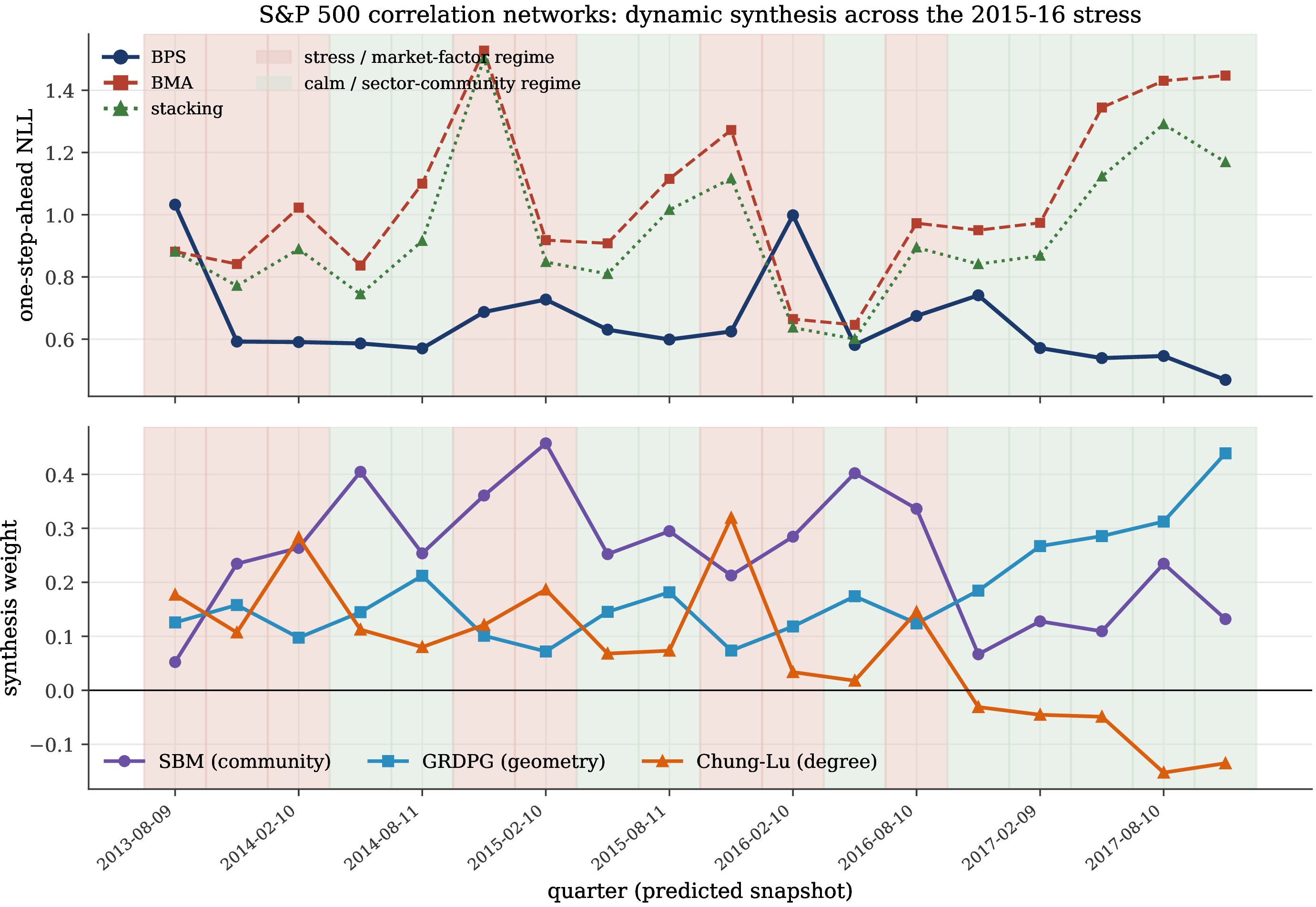
Figure 2 shows the cumulative one-step-ahead log predictive score of the synthesis relative to each combiner, accumulated quarter by quarter [7], [12]. The synthesis has a positive cumulative advantage by the end of the sequence, \(7.1\) nats over model averaging and \(5.2\) over stacking, though individual quarters can favor a competitor.
![Figure 2: Sequential one-step-ahead forecast performance on the S&P network, in the form used to compare density forecasts in Bayesian predictive synthesis [12]: the cumulative log predictive score of the synthesis relative to model averaging and to stacking, accumulated over the eighteen quarterly forecasts. A rising curve means the synthesis places higher predictive density on the realized snapshot at that step; upward segments favor the synthesis and downward segments the comparator.](/article/2606.26136/fig_forecast_lpdr.png "fig:")
We test whether a competitor can match the synthesis by recalibration. Splitting the forecast rounds into a calibration fold (earlier snapshots) and an evaluation fold (later snapshots), we fit isotonic regression on each competitor’s calibration-fold predictions and apply it on the evaluation fold. Recalibration sharply improves the latent-space competitor: its evaluation-fold ECE falls from \(0.244\) to \(0.047\), its NLL from \(0.832\) to \(0.559\), and its \(r=2\) decision cost from \(0.569\) to \(0.401\), while the already-calibrated synthesis improves more modestly (ECE \(0.106\) to \(0.049\)). The recalibrated competitor then matches the synthesis on every forecast score. The synthesis is therefore not uniquely the best forecaster; its advantage is that it delivers calibration together with the mechanism weights, their intervals (Theorem 9), and the localization of Theorem 3, none of which a recalibrated embedding returns.
Refitting the synthesis with the calibration intercept constrained to zero leaves the dense S&P scores essentially unchanged (NLL \(0.653\) to \(0.646\)) but materially degrades the forecast on the sparse Bitcoin-OTC network of the Supplement, so the free calibration layer matters most when the graph is sparse. Fixing the weights (\(\delta=1\)) leaves the average forecast scores unchanged, so the time-varying weights are needed for tracking and localization, not for an average-score gain on a stable panel.
The dynamics also help estimation, in the sparse regime where the single-snapshot theory is weakest. In a stable regime the discounted filter pools recent snapshots to an effective information \(\asymp N_t/(1-\delta)\), lowering the variance of the weight estimate below an independent single-snapshot fit. On a stable three-block model held fixed across snapshots, the filtered community-weight estimate has about half the standard deviation of the single-snapshot fit (Figure 3): at \(N=n^2\rho_n\approx250\) the single-snapshot standard deviation is \(0.25\) and the pooled one \(0.11\), and both shrink as the snapshots densify. The time-varying machinery therefore restores estimable weights where one snapshot is too sparse, and adds little where each snapshot is already dense.

By Theorem 3, the filtered weights localize the active mechanism, which is testable against an external label. From the same daily returns, but independent of the network construction, we compute the realized volatility of the equal-weight market index in each quarter, a standard stress indicator. It agrees with the network’s top-eigenvalue share on the regime (correlation \(0.93\)), and both peak in the 2015–16 stress episode. The volatility series, computed from the returns, is the external validator; the eigenvalue share, read off the correlation matrix itself, is an internal consistency check. The synthesis weights track this regime: the latent-geometry weight is anticorrelated with stress (\(-0.78\) against the external volatility, \(-0.91\) against the internal eigenvalue share) and is largest in the five calm quarters of late 2016–2017; in stress the weight reallocates to the block and degree agents, the block weight leading the most stressed quarters and the degree weight rising most strongly with volatility (\(+0.66\)). The synthesis recovers the regime with no knowledge of the volatility series.
Holding graph density fixed at \(0.10\) in every quarter, by thresholding each correlation matrix at the quantile that yields that density, leaves the synthesis advantage and the weight reallocation intact (NLL \(0.622\) against \(1.14\) for averaging; community weight \(0.40\) in stress against \(0.27\) in calm).
0.0.5.2 Two contact networks with known group labels
We use two dynamic networks that carry known group labels, in different domains. The first is the SocioPatterns high-school face-to-face contact network [60]: wearable sensors recorded close-proximity contacts among \(327\) students of nine classes over five school days in December 2013 at twenty-second resolution. The second is the SocioPatterns hospital-ward network [61]: contacts among \(75\) doctors, nurses, administrative staff, and patients in a Lyon ward over four days, carrying the four role labels. Aggregating each into hourly snapshots on its fixed node set gives \(T=41\) and \(T=44\) snapshots in the sparse regime, on which we run the same one-step-ahead protocol and competitors as above. The class and role labels are held out from every agent and used only for validation.
On both networks the synthesis is the best-calibrated forecaster by a wide margin (Table 3): PIT-KS \(0.107\) and ECE \(0.140\) on the high school and \(0.119\) and \(0.139\) on the hospital, against \(0.29\) to \(0.49\) for the convex combiners, which once again remain badly miscalibrated. Against model averaging the synthesis improves log-score by \(1.45\) on the high school (\(95\%\) CI \([1.31,1.57]\)) and \(1.05\) on the hospital (\([0.90,1.20]\)).
The mechanism weights, which no competitor returns with calibrated uncertainty, are validated against the labels and identify a different mechanism in each domain (Figures 4 and 5). On the high school the community (SBM) weight is largest, near \(0.42\) with an interval that separates from the others at the settled snapshots; the community mechanism is finite-dimensional, so this is the unconditionally valid interval of Theorem 9, and the high school is the case in which the leading mechanism carries the unconditional band. The aggregate contact graph is assortative by class (attribute assortativity \(0.65\) on the held-out labels), with the community agent’s blocks recovering the nine classes almost exactly, adjusted Rand index \(0.993\) and normalized mutual information \(0.994\), computed without the labels; within the school day the community weight rises and falls with the within-class share of contacts (correlation \(0.49\), \(p=0.0015\)), tracking the daily alternation between within-class lessons and between-class mixing. On the hospital the largest weight is instead the degree (Chung–Lu) mechanism, near \(0.50\), whose leading weight is infinite-dimensional and so carries the conditional interval, and the community weight is small. The ward is not assortative by role: its attribute assortativity on the held-out labels is slightly negative (\(-0.12\)), so edges run across roles, not within them and there is no community structure for the SBM to lead on. What organizes the ward is contact volume, and the role labels confirm it, the staff being the hubs (mean aggregate degree \(39\) for nurses and \(36\) for doctors against \(21\) for patients). The synthesis thus reports community structure where it exists and hub structure where that is what dominates, in each case the reading an external label endorses.
These readings, with the S&P regime tracking of Section 0.0.5.1.0.1, are collected in Table 4: the same synthesis names a different mechanism in each network, a held-out signal the agents never see endorses each one, and no competitor returns a comparable mechanism weight with uncertainty.
| Network (\(n\)) | Leading mechanism | Held-out validation |
|---|---|---|
| High school (327) | community / SBM (\(\bar\theta{=}0.42\)) | assortative by the \(9\) classes (\(0.65\)); blocks recover the classes (ARI \(0.993\), NMI \(0.994\)); weight tracks within-class contact share (\(r{=}0.49\), \(p{=}0.0015\)) |
| Hospital ward (75) | degree / Chung–Lu (\(\bar\theta{=}0.50\)) | not assortative by the \(4\) roles (\(-0.12\)); staff are the hubs (mean degree: nurses \(39\), doctors \(36\), vs patients \(21\)) |
| S&P 500 (470) | geometry / GRDPG, regime-tracking | realized volatility (external): geometry weight \(r{=}-0.78\) (\(-0.91\) vs eigenvalue share); block and degree rise in stress, degree \(r{=}+0.66\) |


0.0.5.3 Controlled simulations
We simulate \(T=12\) snapshots on \(n=300\) nodes in three regimes of four snapshots each: a community regime (a three-block SBM), a hub regime (a Chung–Lu power-law degree model), and a geometry regime (a two-dimensional GRDPG). This is a controlled setting in which the data-generating mechanism changes abruptly, and it is the natural test of whether the synthesis can track. Table 5 reports averages over the eleven one-step forecasts.
| Method | NLL | PIT-KS | ECE |
|---|---|---|---|
| Dynamic BPS | 0.742 | 0.074 | 0.108 |
| BMA | 1.443 | 0.401 | 0.433 |
| Stacking | 1.383 | 0.391 | 0.426 |
| Equal weight | 1.378 | 0.389 | 0.426 |
| SBM agent | 1.427 | 0.403 | 0.432 |
| GRDPG agent | 2.338 | 0.365 | 0.417 |
| Chung–Lu agent | 1.430 | 0.400 | 0.431 |
The synthesis roughly halves the NLL of every competitor (NLL \(0.74\) versus \(1.38\)–\(2.34\)) and improves calibration by a factor of five (PIT-KS \(0.074\) versus \(0.39\)–\(0.40\)). The per-regime synthesis log-scores are stable (\(0.83\) community, \(0.70\) hub, \(0.71\) geometry), showing that no single regime is responsible for the gain.
The filtered log-score and weights reflect the regime structure. The one-step log-score spikes at each regime change (snapshots \(t=4\) and \(t=8\)) and re-adapts within the regime, whereas BMA and stacking remain high throughout, and the filtered weights reallocate in step: in the community regime the SBM weight is large (\(\approx 0.9\)); at the switch to the hub regime the Chung–Lu weight rises from \(0.12\) to \(0.75\) while SBM is discounted; and the weights move again at the geometry switch.
Theorem 3 sharpens this into a localization claim: when a mechanism is active with a positive margin, the largest filtered weight should name it. Scoring the argmax of the filtered structural weights against the active regime across the eleven forecasts, the synthesis localizes correctly in \(6\) of \(11\) snapshots, and the pattern is exactly what the margin condition predicts. In the community regime the SBM weight is largest at all three forecasts (\(3/3\)); in the hub regime Chung–Lu is largest at three of four, the single miss being the first snapshot after the switch, which is the recovery delay \(h\) of the theorem made visible. In the geometry regime the GRDPG weight is not the largest in any of the four geometry-regime forecasts. The latent-geometry signal in this simulation is weakly separated from degree heterogeneity, so the margin \(\kappa\) is small and the localization condition of Theorem 3 fails. This is consistent with the theorem, which guarantees localization only above the margin; and the design-conditioning diagnostic of Section 0.0.5.3.0.7 is what tells a practitioner in advance which regimes are separable. Calibration, by contrast, does not depend on the margin and remains strong throughout (PIT-KS \(0.074\)).
Theorem 3 guarantees localization only above the margin, so the geometry failure above should be a small-margin artifact, not a structural limit. We confirm this with the same three-regime design at a large, well-separated per-dyad contrast (\(\kappa=2.2\)), with the three signals made mutually distinct: assortative blocks for community, latent positions on the unit sphere for geometry (unit norm, so the geometry signal carries no degree information and the earlier aliasing is removed), and an expected-degree product for degree. Over thirty replications, at the settled snapshot of each regime the largest synthesis weight lands on the truly active mechanism in every case, a localization hit rate of \(1.00\) for all three mechanisms, geometry included (Figure 6); the only misses fall in the one or two snapshots immediately after a switch, the recovery delay \(h\) of the theorem, which lowers the all-snapshot rate to \(0.58\) and \(0.60\) for the two regimes that follow a switch. Localization therefore succeeds for every mechanism once its margin clears the threshold, exactly as Theorem 3 predicts, and the weak-margin geometry failure is the predicted small-\(\kappa\) regime, not a limitation of the synthesis.

Remark 2 makes the gap over averaging rules quantitative: after a regime of length \(L\), vanilla Bayesian model averaging has accumulated \(\Theta(L)\) log-odds of evidence for the old mechanism and needs an \(\Omega(L)\)-long window to reverse, whereas the discounted synthesis forgets in \(O(1/(1-\delta))\) snapshots independent of \(L\). Dynamic model averaging [53] introduces a forgetting factor to reduce this inertia, so we include it with forgetting matched to the synthesis discount, alongside vanilla averaging. A network switches once from a community regime (an SBM) to a hub regime (a Chung–Lu degree model) after \(L\) snapshots, and we record, for each method, the recovery delay, the number of post-switch snapshots until its largest combination weight points to the new mechanism. Varying \(L\) from \(2\) to \(16\) and averaging over eight replications, Figure 7 (center) reports the recovery delay. The synthesis recovers in a constant single snapshot at every \(L\) (delay slope \(0.00\)). Vanilla averaging takes longer the longer the old regime lasted, its delay rising from near zero at \(L=2\) to nineteen snapshots at \(L=16\) (slope \(1.39\)), one extra snapshot of lag per snapshot of history. Dynamic model averaging falls between the two: its forgetting factor bounds the inertia, so the delay plateaus near six snapshots, not growing without limit (slope \(0.43\)), but it still does not match the synthesis, because it remains an averaging rule that must accumulate \(O(1/(1-\delta))\) snapshots of new-regime evidence to overcome the evidence it has retained, whereas the synthesis carries an unconstrained logit state with an intercept and relocates at once.
Theorem 3 bounds the filter’s cumulative one-step-ahead regret against the per-snapshot oracle by 9 , whose only series-growing term is the comparator movement, itself controlled by the number of switches. At a fixed horizon the cumulative regret rises monotonically with the number of switches, from \(0.68\) at none to \(1.62\) at six (slope \(0.16\) per switch, tracking a movement budget that climbs from \(0.5\) to \(13\)), while holding switches at zero and quadrupling the horizon leaves it essentially flat (\(0.69\) at \(T=10\), \(0.74\) at \(T=44\)): the filter charges per switch, not per time point, exactly as 9 predicts.
0.0.5.3.0.1 The localization threshold.
By Theorem 3, the filter localizes the active mechanism only above a contrast threshold: the localization delay is of order \(\log J/(N_t\kappa^2)\), so a settled regime is identifiable once \(\kappa\) exceeds \(\sqrt{\log J/N_t}\). We confirm this on a synthetic sequence that alternates a community and a degree regime at a controlled contrast \(\kappa\), with the geometry agent present as a distractor. The settled localization hit rate is near the chance level \(1/J\) for small \(\kappa\) and reaches one for \(\kappa\ge0.75\). The crossing lies a constant factor above the information floor \(\sqrt{\log J/(N_t\rho(1-\rho))}\approx0.11\), the one-snapshot agent-estimation term \(a_{n,t}\) of 9 . The per-snapshot average saturates lower, near \(0.63\), because each switch costs a snapshot or two of relocalization.
0.0.5.3.0.2 The dyadic rate.
Theorem 1 predicts that the synthesis weights are estimable from a single snapshot with standard error \((n^2\rho_n)^{-1/2}\). Subsampling induced subgraphs of the densest S&P snapshot (November 2015, \(55{,}214\) edges) and refitting the one-snapshot synthesis on each, the empirical standard error of the fitted weights falls along the dyadic rate (Figure 7, left): a fitted log-log slope of \(-0.535\) against the theoretical \(-1/2\), the weight standard deviation shrinking from \(0.18\) to \(0.018\) as the edge information grows sixty-six-fold. The same decay appears on the full snapshots, where the latent-geometry weight is pinned to standard error \(0.03\) on the stressed November 2015 graph but carries errors five to twenty times larger on the sparse November 2017 graph (\(1{,}986\) edges). The rate is a property of one graph, not of the series.

0.0.5.3.0.3 Coverage and normality of the weights.
The rate is one half of Theorem 1; the other half is the conditional normal limit 8 with the sandwich variance, which is what licenses confidence intervals for the weights. We test it in a controlled design where the population weight is known. Two fixed agent surfaces, a three-block community logit and a degree logit, are combined at a known weight \(\boldsymbol{\beta}^\circ=(\alpha,\theta_{\mathrm{comm}},\theta_{\mathrm{deg}})\) with a \(\log\rho_n\) offset, and we sample many graphs from the resulting edge law, refit the dyadic logistic regression on each, and form the inverse-information Wald intervals. Over \(400\) replications at \(n=300\) (\(N_t\approx3{,}900\)), the empirical coverage of the nominal \(95\%\) intervals is \(96.3\%\) for the intercept, \(95.8\%\) for the community weight, and \(95.8\%\) for the degree weight, and the standardized estimates \((\widehat\beta-\beta^\circ)/\mathrm{se}\) are indistinguishable from a standard normal (Kolmogorov–Smirnov statistics \(0.049\), \(0.022\), \(0.029\)). The standard error of the community weight falls along \(N_t^{-1/2}\) with a fitted log-log slope of \(-0.500\), the dyadic rate exactly. The intercept here is centered at \(\log\rho_n+\alpha\), a direct illustration of the sparsity offset: without it the intercept silently absorbs the density. With the agent surfaces known, the conditional limit of Theorem 1 holds with valid coverage at the predicted rate.
This coverage is conditional on the agents, and Theorem 1 is explicit that the unconditional limit requires \(\sqrt{N_t}\,a_{n,t}\to0\), a condition the SBM agent rate violates in the denser part of the sparsity regime. We measure the cost directly. Refitting the community and degree agents on each sampled graph and forming the same naive inverse-information intervals, the coverage of the community weight falls below nominal and the shortfall grows with the edge information: from \(82\%\) at \(N_t\approx2{,}700\) to \(71\%\) at \(N_t\approx43{,}000\), while the standardized bias rises from \(0.5\) to \(1.1\) standard errors over the same range. The fixed-agent coverage stays at nominal throughout, so the gap is entirely the agent-estimation error entering the weight limit at first order. The naive single-snapshot intervals are thus valid when the agents are known or estimated at a negligible rate and undercover when a flexible agent is refit on the same dense graph; the cross-fold orthogonal estimator of Theorem 9 closes this gap, with an unconditional limit valid under an \(o(N_t^{-1/4})\) agent rate.
0.0.5.3.0.4 The cross-fold orthogonal correction.
Theorem 9 asserts that a cross-fold Neyman-orthogonal score restores an unconditional normal limit, and valid intervals, under a mild agent rate; we confirm this on a design where the orthogonal correction is exactly constructed. A known three-block community surface carries the target weight, while the degree mechanism is the refit nuisance, estimated on each graph by a regularized Fourier sieve in a node-pair covariate, and the blocks carry distinct degree levels, so the target and the nuisance are correlated and a mis-estimated nuisance contaminates the target. The naive plug-in, which treats the fitted sieve as known and inverts the second-stage information, undercovers the community weight: the empirical coverage of the nominal \(95\%\) interval lies between \(82\%\) and \(94\%\), with a standardized bias as large as one standard error where the nuisance bias is strongest. The cross-fold orthogonal estimator, which partials the target against the nuisance basis out of fold and forms the orthogonal sandwich, holds nominal coverage of \(96\%\) to \(98\%\) with a standardized bias below \(0.15\) across the whole range of edge information, from \(N_t\approx2{,}700\) to \(N_t\approx43{,}200\). The orthogonal coverage neither drifts nor degrades as the graph grows, which is the unconditional limit of Theorem 9 made visible: the debiasing yields valid confidence statements for an individual mechanism weight at the price of one cross-fold construction.
0.0.5.3.0.5 The separation rate.
Theorem 2 predicts a separation rate \(\Delta_n\asymp(n^2\rho_n)^{-1/2}\) in graphon log-odds, the boundary between distinguishable and indistinguishable mechanisms. Sweeping the log-odds contrast \(\delta\) and locating the boundary \(n^2\rho_n^\ast\) at which power crosses \(0.9\), the boundary falls from \(683\) to \(39\) as \(\delta\) grows from \(0.10\) to \(0.43\) (Figure 7, right), a fitted log-log slope of \(-1.93\) against the predicted \(-2\). Every real snapshot, the S&P graphs (\(1{,}986\) to \(55{,}214\) edges) and the co-occurrence graphs (\(700\) to \(1{,}000\)), lies well inside the detectable region, the boundary sitting at vanishing contrast within the sparsity regime. The matching impossibility below the rate is Theorem 2 itself, by the sparse-logit lemma and the two-point method.
0.0.5.3.0.6 Dominance over model averaging under misspecification.
Under misspecification a coherent Bayesian model-averaging posterior concentrates on the single Kullback–Leibler-closest agent as edge information accumulates, its weight vector tending to \((1,0,0)\): this is Berk’s collapse, the correct behavior of a posterior but the wrong default for combination, since it discards the other agents instead of reweighting them. The synthesis instead retains and reweights all agents, and Theorem 4 makes the resulting log-score gap 11 strictly positive whenever the truth is not a single agent. In this misspecified setting the gap is positive on every study, ranging from \(0.39\) on the S&P network to \(3.33\) on the power-grid mesh; Figure 9 in the Supplement plots the gap and the entropy collapse.
0.0.5.3.0.7 Mechanism aliasing.
By Theorem 1, two mechanisms are indistinguishable from a snapshot exactly when the dyad-feature information matrix \(H_t\) is singular. Its condition number \(\kappa(H_t)\) is an observable diagnostic of how close two mechanisms are to aliasing. The controls behave as predicted: a degree-corrected block model, whose community and degree agents are distinct, is far better conditioned (\(\kappa\approx340\)) than the near-aliased control, whereas a structureless Erdős–Rényi graph, where both agents collapse to a constant and alias, is roughly six times worse. The real networks span four orders of magnitude, from the dense S&P stress snapshot (\(\kappa\approx6\)), where distinct community, geometry, and degree signals make the weights sharply separable and underwrite the precise estimates of Section 0.0.5.3.0.2, to the extremely sparse ca-GrQc (\(\kappa\approx7.8\times10^4\)), which approaches aliasing, so that individual weights there are only weakly identified even where the pooled forecast is accurate.
0.0.5.4 Large dynamic networks
The networks so far have a few hundred to a few thousand active nodes. To probe scale and out-of-sample behavior we apply the same synthesis model, with the data construction and evaluation adapted for scale (symmetrization, balanced dyad sampling, and recent-history pruning, described below), to two large public timestamped networks [62] on their entire node sets: the arXiv HEP-PH citation network [63] (\(n=28{,}093\), \(T=85\) monthly snapshots), the Enron e-mail network [64] (\(n=86{,}978\), \(T=46\)). The HEP-PH citation and Enron e-mail logs are natively directed; because the model and theory of Section 0.0.2 are defined for undirected graphs, we symmetrize each to fit the undirected observation model, placing an undirected edge between two nodes joined by at least one citation, message, or interaction within a snapshot and discarding the directional signal. The full dyad set is too large to score at these node counts. Each forecast is therefore evaluated on a balanced dyad sample of all edges and an equal number of randomly sampled non-edges. The sparse offset maps the sample probabilities to the population scale as in Corollary 1, and all methods are scored on this common balanced sample. The three mechanism agents are fit on the discounted-average adjacency through \(t-1\), so they are the dynamic block, latent-geometry, and degree predictors used as competitors in the S&P study (Section 0.0.5.1.0.1) and match the history-based agent definition of Section 0.0.2. At this scale the discounted-average adjacency is pruned to its recent-history window so that the largest graph fits in memory.
Two findings carry over to this scale (Table 6, Figure 8). First, the synthesis is the best-calibrated method on both networks, with PIT deviation \(0.031\) to \(0.061\) and calibration error \(0.041\) to \(0.077\), against \(0.41\) to \(0.50\) for every classical combiner and single agent; on the log-score it is lowest among the compared methods on both networks, by \(2.5\) to \(3.5\) nats per dyad. Second, the weights remain tightly estimated at this scale: they favor degree and community on the citation network, with the geometry weight near zero, and are positive across all three mechanisms on the e-mail network. The two networks fall in different regimes: on the citation network the synthesis is calibrated and predictive, whereas the e-mail network sits in the near-base-rate regime of Corollary 1, where the edge probabilities are nearly uniform and the synthesis delivers calibration without discrimination.
| Method | NLL | PIT-KS | ECE |
|---|---|---|---|
| arXiv HEP-PH (\(n=28{,}093\), \(T=85\)) | |||
| Dynamic BPS | 0.413 | 0.031 | 0.041 |
| BMA | 3.032 | 0.457 | 0.486 |
| Stacking | 2.937 | 0.448 | 0.484 |
| Equal weight | 3.081 | 0.449 | 0.487 |
| SBM agent | 3.030 | 0.457 | 0.486 |
| GRDPG agent | 3.855 | 0.424 | 0.479 |
| Chung–Lu agent | 3.945 | 0.470 | 0.495 |
| Enron e-mail (\(n=86{,}978\), \(T=46\)) | |||
| Dynamic BPS | 0.597 | 0.061 | 0.077 |
| BMA | 4.508 | 0.451 | 0.488 |
| Stacking | 4.125 | 0.447 | 0.488 |
| Equal weight | 4.163 | 0.457 | 0.491 |
| SBM agent | 4.672 | 0.495 | 0.499 |
| GRDPG agent | 4.510 | 0.431 | 0.479 |
| Chung–Lu agent | 4.615 | 0.474 | 0.496 |
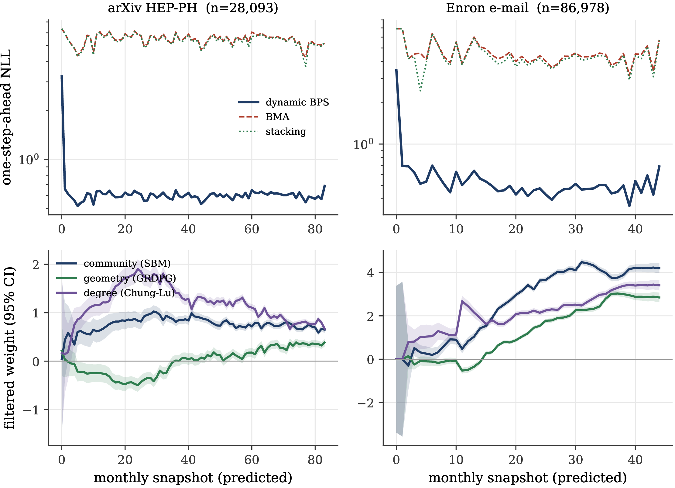
We also evaluate the one-step-ahead point forecasts by mean squared forecast error (MSFE\(_{1:T}\), the Brier score for a binary edge on the balanced evaluation set of all edges and an equal-sized random sample of non-edges). The synthesis attains \(0.112\) and \(0.165\) on the citation and e-mail networks; the classical combiners lie near \(0.47\) to \(0.50\) on both, worse by \(185\%\) to \(345\%\), so the calibration advantage is also a point-forecast advantage.
0.0.6 Discussion and limitations↩︎
We developed dynamic Bayesian predictive synthesis for dynamic networks. Each generative mechanism, such as community structure, latent geometry, or degree heterogeneity, is treated as an agent that forecasts the next snapshot’s edges, and a synthesis layer combines these forecasts with weights that form the state of a dynamic linear model. The weights are the object of inference: the method jointly estimates which mechanism is most informative at each time and produces a calibrated forecast, specializing to calibrated link prediction at a single snapshot. Because a network on \(n\) nodes has of order \(n^2\) node pairs, one snapshot estimates the weights precisely even when the graph is sparse, and faster than the mechanisms change. Conditional on the fitted agents the intervals hold at the dyadic rate; for finite-dimensional agents a cross-fold orthogonal construction removes the refitting bias and makes them unconditional, while for high-dimensional latent-position and degree agents they remain conditional. Two mechanisms separate only above a sharp contrast threshold; a change in the active mechanism is tracked at a cost paid only at the change, at a minimax-optimal rate; and when no agent is correct the weight converges to the projection of the active mechanism onto the set of agents while the forecast stays calibrated, where model averaging collapses onto a single mechanism.
The empirical studies support these results. On real dynamic networks the estimated weights track regime changes identified independently of the model; the synthesis remains calibrated where model averaging collapses and pooling miscalibrates; and its advantage is largest at the regime changes the theory identifies. The contribution is a single model that produces calibrated forecasts without a separate recalibration step, together with interpretable time-varying mechanism weights that carry conditional intervals, unconditional for finite-dimensional mechanisms, and identify mechanism changes. A forecaster that is not mechanism-based can be recalibrated to match the probabilities, but does not provide the weights or their uncertainty.
The results rest on two modeling choices: a finite, fixed set of agents, and an undirected binary observation model with conditionally independent dyads. Enlarging the set of agents leaves the filter unchanged but slows the estimation rate to \(\{(n^2\rho_n)/J_t\}^{-1/2}\) and raises the separation threshold. The conditionally independent dyad assumption holds only approximately for the main-text networks, so the weight inference is validated on matched simulations and reported with a dependence-robust variance.
We propose three extensions. First, weighted or count-valued edges replace the Bernoulli model with a Gaussian or Poisson one. Directed and signed networks require asymmetric observation models and are left to future work: the citation and e-mail networks studied here are natively directed and are symmetrized to fit the undirected model, so a native-directed analysis, which must also model the reciprocity-induced dependence between the two orientations of a dyad, is a genuine extension and not a relabeling. The projection and tracking arguments extend to any observation model with a smooth log-likelihood, but the directed case is not immediate. Second, the Laplace filter can be replaced by particle filtering when a network snapshot is too sparse for the Gaussian approximation. Third, the dynamic block-model and latent-space forecasters used here as benchmarks [35]–[38] can be folded into the set of agents.
Acknowledgments↩︎
The authors thank colleagues for helpful discussions. Code to reproduce all results is provided with this manuscript.
Disclosure Statement↩︎
The authors report there are no competing interests to declare.
Data Availability Statement↩︎
All networks analyzed in this article are publicly available benchmark datasets. The main text uses a financial correlation network built from public daily S&P 500 prices (Section 0.0.5.1.0.1); the SocioPatterns high-school and hospital-ward face-to-face contact networks [60], [61]; and two large public timestamped networks [62], the arXiv HEP-PH citation network [63] and the Enron e-mail network [64]. The Supplement additionally analyzes the Bitcoin-OTC trust network [65], [66] and standard static link-prediction benchmarks, including the ca-GrQc and ca-CondMat collaboration networks [63], the political-blogs network [67], and the Western-states power-grid network [68]. Code reproducing all simulations, tables, and figures, together with the scripts that construct each snapshot set from its public source, is openly available at https://osf.io/fer69/overview?view_only=6f79f15628084adcb253f98b127d4649.
Supplementary Material↩︎
This supplement contains the complete statements and proofs of the results of Section 4 of the main text and of the two further inferential and tracking results. Section 0.0.7 proves the single-snapshot identification, aliasing, and dyadic central limit theorem (Theorem 1). Section 0.0.8 proves the sparse Bernoulli-logit perturbation lemma and the separation rate (Theorem 2). Section 0.0.9 proves the point-prequential tracking, switch-recovery, and localization theorem (Theorem 3). Section 0.0.10 proves the projection, calibration, model-averaging collapse, and stacking-gap theorem (Theorem 4). Section 0.0.11 proves the static cross-fitted synthesis corollary (Corollary 5). Section 0.0.12 proves the cross-fold orthogonal unconditional limit (Theorem 1c), and Section 0.0.13 proves the local minimax lower bound for mechanism tracking (Theorem 3b). Numbering of equations and constants is local to each section; the constant \(C\) may change from line to line.
0.0.6.0.0.1 Notation.
Notation matches the main text. The population log-odds projection of the network onto the set of mechanism agents, written \(\boldsymbol{\beta}^\circ_t\) in the main text, is denoted \(\bar\boldsymbol{\beta}_{t,n}\) here; its oracle, error-free-agent counterpart is \(\boldsymbol{\beta}^{\mathrm{or}}_{t,n}\). The synthesis dimension is \(d=J+1\); coefficient vectors are written in non-bold type; and a subscript \(n\) or \(t,n\) makes the dependence on the snapshot size explicit. The information scale \(N_{t,n}\), the normalized information matrix \(H_{t,n}\), the dyad feature \(z_{t,e}= (1,u^{(1)}_{t,e},\dots,u^{(J)}_{t,e})^{\!\top}\), the sparse offset \(\log\rho_n\), and the four mechanism agents (block, geometry, degree, local) are exactly the objects of Section 4.
0.0.7 Single-snapshot synthesis: identification, aliasing, and dyadic limit↩︎
Theorem 5 (Single-snapshot synthesis: identification, aliasing, and dyadic limit). Fix \(t\) and let \(n\to\infty\). Let \(\mathcal{E}_{t,n}\) be the dyads used in the time-\(t\) synthesis update and write \[m_{t,n}=|\mathcal{E}_{t,n}|.\] For \(e\in\mathcal{E}_{t,n}\), put \[Y_{t,e}=A_{t,e}, \qquad z_{t,e} = (1,u^{(1)}_{t,e},\ldots,u^{(J)}_{t,e})^\top \in\mathbb{R}^d, \qquad d=J+1 .\] For the rate and central limit theorem below, \(d\) is fixed. Let \(\ell_{\rho,n}=\log\rho_n\) and define the sparse-offset synthesis probabilities \[\eta_{t,e}(\boldsymbol{\beta}) = \ell_{\rho,n}+\boldsymbol{\beta}^\top z_{t,e}, \qquad q_{t,e}(\boldsymbol{\beta}) = \sigma\{\eta_{t,e}(\boldsymbol{\beta})\}, \qquad \sigma(x)=\frac{e^x}{1+e^x}.\] Let \(\mathcal{F}_{t,n}\) be the sigma-field generated by the history, the cross-fitted agents, the sampled dyad set \(\mathcal{E}_{t,n}\), the offset \(\ell_{\rho,n}\), and the true conditional edge-probability array \(p_{t,e}=\mathbb{P}(Y_{t,e}=1\mid \mathcal{F}_{t,n})\). Assume that the dyad set is conditionally non-informative for the edge outcomes: conditional on \(\mathcal{F}_{t,n}\), \(Y_{t,e}\sim {\rm Bernoulli}(p_{t,e})\), \(e\in\mathcal{E}_{t,n}\), independently over \(e\). Outcome-dependent case-control sampling is excluded from this theorem unless the corresponding retrospective logit correction is included in the likelihood. Assume the following basic conditions.
The parameter space \(\Theta\subset\mathbb{R}^d\) is compact, convex, and full-dimensional.
The fitted-agent design is uniformly bounded: \(\max_{e\in\mathcal{E}_{t,n}}\|z_{t,e}\|\le B<\infty\).
The sparse scale is preserved uniformly on \(\Theta\): there exist constants \(0<c_q<C_q<\infty\) such that, for all sufficiently large \(n\), \(c_q\rho_n\le q_{t,e}(\boldsymbol{\beta})\le C_q\rho_n\le \tfrac12\) for all \(e\in\mathcal{E}_{t,n},\;\boldsymbol{\beta}\in\Theta\). The true probabilities are on the same sparse scale, \(0\le p_{t,e}\le C_p\rho_n\), and \(m_{t,n}\rho_n\to\infty\).
Define the conditional fitted-agent population risk \[R_{t,n}(\boldsymbol{\beta}) = \sum_{e\in\mathcal{E}_{t,n}} \left[ \log\{1+\exp(\eta_{t,e}(\boldsymbol{\beta}))\} - p_{t,e}\eta_{t,e}(\boldsymbol{\beta}) \right],\] and the pseudo-true set \(\mathcal{B}_{t,n}=\arg\min_{\boldsymbol{\beta}\in\Theta}R_{t,n}(\boldsymbol{\beta})\). For any \(\boldsymbol{\beta}\in\Theta\), let \(w_{t,e}(\boldsymbol{\beta})=q_{t,e}(\boldsymbol{\beta})\{1-q_{t,e}(\boldsymbol{\beta})\}\), \(N_{t,n}(\boldsymbol{\beta})=\sum_{e}w_{t,e}(\boldsymbol{\beta})\), and \(H_{t,n}(\boldsymbol{\beta})=N_{t,n}(\boldsymbol{\beta})^{-1}\sum_{e}w_{t,e}(\boldsymbol{\beta})z_{t,e}z_{t,e}^\top\).
- Let \(\mathcal{N}_{t,n}=\{a\in\mathbb{R}^d: a^\top z_{t,e}=0 \;\forall e\in\mathcal{E}_{t,n}\}\). Because \(w_{t,e}(\boldsymbol{\beta})>0\), \({\rm Null}\{H_{t,n}(\boldsymbol{\beta})\}=\mathcal{N}_{t,n}\) for every \(\boldsymbol{\beta}\in\Theta\). Hence the conditional synthesis law \(\boldsymbol{\beta}\mapsto\{q_{t,e}(\boldsymbol{\beta}):e\in\mathcal{E}_{t,n}\}\) is identified on \(\Theta\) if and only if \(\mathcal{N}_{t,n}=\{0\}\), equivalently if and only if \(H_{t,n}(\boldsymbol{\beta})\) is full rank for one, and hence for every, \(\boldsymbol{\beta}\in\Theta\). If \(\mathcal{N}_{t,n}\neq\{0\}\), then \(\boldsymbol{\beta}\) is identified only modulo \(\mathcal{N}_{t,n}\), and a linear functional \(a^\top\boldsymbol{\beta}\) is identifiable if and only if \(a\in\mathcal{N}_{t,n}^\perp={\rm Range}\{H_{t,n}(\boldsymbol{\beta})\}\). Thus exact affine dependence among \(1,u^{(1)}_{t,\cdot},\ldots,u^{(J)}_{t,\cdot}\) aliases the corresponding separate agent weights.
For the estimation and CLT statements, add:
The pseudo-true set has a uniformly interior representative \(\bar\boldsymbol{\beta}_{t,n}\in\mathcal{B}_{t,n}\) with \({\rm dist}(\bar\boldsymbol{\beta}_{t,n},\partial\Theta)\ge c_\Theta>0\); hence \(\Psi_{t,n}(\bar\boldsymbol{\beta}_{t,n})=0\), where \(\Psi_{t,n}(\boldsymbol{\beta})=\sum_{e}\{p_{t,e}-q_{t,e}(\boldsymbol{\beta})\}z_{t,e}\).
The fixed-design Gram matrix \(G_{t,n}=m_{t,n}^{-1}\sum_e z_{t,e}z_{t,e}^\top\) satisfies \(\lambda_{\min}(G_{t,n})\ge g>0\). Write \(N_{t,n}=N_{t,n}(\bar\boldsymbol{\beta}_{t,n})\), \(H_{t,n}=H_{t,n}(\bar\boldsymbol{\beta}_{t,n})\).
With \(V_{t,n}=N_{t,n}^{-1}\sum_e p_{t,e}(1-p_{t,e})z_{t,e}z_{t,e}^\top\), assume \(H_{t,n}\to H_t\) and \(V_{t,n}\to V_t\) with \(H_t\) nonsingular.
Let \(\hat{\boldsymbol{\beta}}_{t,n}\) minimize \(\ell_{t,n}(\boldsymbol{\beta})+P_{t,n}(\boldsymbol{\beta})\), where \(\ell_{t,n}(\boldsymbol{\beta})=\sum_e[\log\{1+\exp(\eta_{t,e}(\boldsymbol{\beta}))\}-Y_{t,e}\eta_{t,e}(\boldsymbol{\beta})]\) and \(P_{t,n}\) is an \(\mathcal{F}_{t,n}\)-measurable, twice continuously differentiable negative log-prior or penalty. For the MLE, \(P_{t,n}\equiv0\); for a weak MAP estimator, \(\|\nabla P_{t,n}(\bar\boldsymbol{\beta}_{t,n})\|=o(\sqrt{N_{t,n}})\) and \(\sup_{\boldsymbol{\beta}\in\Theta}\|\nabla^2P_{t,n}(\boldsymbol{\beta})\|_{\rm op}=o(N_{t,n})\).
Then, conditionally on \(\mathcal{F}_{t,n}\):
\(\|\hat{\boldsymbol{\beta}}_{t,n}-\bar\boldsymbol{\beta}_{t,n}\|=O_{\mathbb{P}}(\sqrt{(J+1)/N_{t,n}})\). Under (B3), \(N_{t,n}\asymp m_{t,n}\rho_n\); hence for a full undirected snapshot with \(m_{t,n}\asymp n^2\), \(\|\hat{\boldsymbol{\beta}}_{t,n}-\bar\boldsymbol{\beta}_{t,n}\|=O_{\mathbb{P}}(\sqrt{(J+1)/(n^2\rho_n)})\).
The estimator has the conditional asymptotic linear representation \[\sqrt{N_{t,n}}(\hat{\boldsymbol{\beta}}_{t,n}-\bar\boldsymbol{\beta}_{t,n}) = H_{t,n}^{-1}N_{t,n}^{-1/2} \sum_{e\in\mathcal{E}_{t,n}}(Y_{t,e}-p_{t,e})z_{t,e}+o_{\mathbb{P}}(1),\] and consequently \(\sqrt{N_{t,n}}(\hat{\boldsymbol{\beta}}_{t,n}-\bar\boldsymbol{\beta}_{t,n})\Rightarrow N(0,H_t^{-1}V_tH_t^{-1})\). If the Bernoulli-logit model is correctly specified, \(p_{t,e}=q_{t,e}(\bar\boldsymbol{\beta}_{t,n})\) for every \(e\), then \(V_{t,n}=H_{t,n}\), so the limit reduces to \(N(0,H_t^{-1})\).
If the arrays \(\mathcal{F}_{t,n},\{z_{t,e}\},\{p_{t,e}\},\mathcal{E}_{t,n}\) are random, the convergence is quenched: for every deterministic sequence satisfying the assumptions the conditional law converges as stated, and if the assumptions hold with probability tending to one and \(H_{t,n},V_{t,n}\) converge in probability, then the conditional bounded-Lipschitz distance to the stated Gaussian limit converges to zero in probability. Finally, let \(\boldsymbol{\beta}^{\mathrm{or}}_{t,n}\) denote an oracle pseudo-true target based on population, error-free agent surfaces, and suppose \(N_{t,n}^{-1}\sup_{\boldsymbol{\beta}\in\Theta}\|\Psi^{\rm fit}_{t,n}(\boldsymbol{\beta})-\Psi^{\rm or}_{t,n}(\boldsymbol{\beta})\| =O_{\mathbb{P}}(a_{n,t})\) and \(-N_{t,n}^{-1}\dot{\Psi}^{\rm or}_{t,n}(\boldsymbol{\beta})\succeq\lambda_{\rm or}I_d\) on the segment between \(\bar\boldsymbol{\beta}_{t,n}\) and \(\boldsymbol{\beta}^{\mathrm{or}}_{t,n}\). Then \(\|\bar\boldsymbol{\beta}_{t,n}-\boldsymbol{\beta}^{\mathrm{or}}_{t,n}\|=O_{\mathbb{P}}(a_{n,t})\). If \(\|\tilde{\boldsymbol{\beta}}_{t,n}-\hat{\boldsymbol{\beta}}_{t,n}\|=O_{\mathbb{P}}(r_{\rm Lap})\), then \[\|\tilde{\boldsymbol{\beta}}_{t,n}-\boldsymbol{\beta}^{\mathrm{or}}_{t,n}\| = O_{\mathbb{P}}\big(\sqrt{(J+1)/N_{t,n}}+a_{n,t}+r_{\rm Lap}\big).\] An oracle-centered CLT with the same covariance holds under \(\sqrt{N_{t,n}}\{a_{n,t}+r_{\rm Lap}\}\to0\); without it the valid normal approximation is centered at \(\bar\boldsymbol{\beta}_{t,n}\), not \(\boldsymbol{\beta}^{\mathrm{or}}_{t,n}\).
Proof. All probability statements in the main part of the proof are conditional on \(\mathcal{F}_{t,n}\). Thus the dyad set, the fitted-agent features, the sparse offset, and the true probability array are fixed. We suppress \(t\) from the notation when no confusion is possible. Conditional on \(\mathcal{F}_{t,n}\), the variables \(\{Y_e:e\in\mathcal{E}_n\}\) are independent Bernoulli with success probabilities \(p_e\). Since the dyad sample is conditionally non-informative, the ordinary Bernoulli likelihood is the correct conditional likelihood. We first prove identification. Because \(\sigma\) is strictly increasing, \(q_e(\boldsymbol{\beta})=q_e(\boldsymbol{\beta}')\) for every \(e\in\mathcal{E}_n\) if and only if \((\boldsymbol{\beta}-\boldsymbol{\beta}')^\top z_e=0\) for every \(e\). For any \(\boldsymbol{\beta}\in\Theta\) and \(a\in\mathbb{R}^d\), \[a^\top H_n(\boldsymbol{\beta})a = N_n(\boldsymbol{\beta})^{-1}\sum_{e\in\mathcal{E}_n}w_e(\boldsymbol{\beta})(a^\top z_e)^2 .\] Since \(w_e(\boldsymbol{\beta})>0\), this equals zero if and only if \(a^\top z_e=0\) for every \(e\). Therefore \({\rm Null}\{H_n(\boldsymbol{\beta})\}=\mathcal{N}_n\), and the map \(\boldsymbol{\beta}\mapsto\{q_e(\boldsymbol{\beta})\}\) is injective on \(\Theta\) iff \(\mathcal{N}_n=\{0\}\), i.e. iff \(H_n(\boldsymbol{\beta})\) is full rank. If \(a\in\mathcal{N}_n\), then \(q_e(\boldsymbol{\beta}+sa)=q_e(\boldsymbol{\beta})\) for every feasible \(s\) and \(e\), so the likelihood and risk are constant along feasible null-space directions, whence \(\boldsymbol{\beta}\) is identified only modulo \(\mathcal{N}_n\). A linear functional \(b^\top\boldsymbol{\beta}\) is constant on \(\boldsymbol{\beta}+\mathcal{N}_n\) iff \(b\perp\mathcal{N}_n\), i.e. \(b\in\mathcal{N}_n^\perp= {\rm Range}\{H_n(\boldsymbol{\beta})\}\). An affine dependence among the agent dyad-logit surfaces is a nonzero \(c\) with \(c^\top z_e=0\) for every \(e\), i.e. \(c\in\mathcal{N}_n\); the corresponding separate weights are aliased. This proves (a). We now prove the rate and the CLT. By (B3), \(q_e(\boldsymbol{\beta})\{1-q_e(\boldsymbol{\beta})\}\asymp\rho_n\) uniformly over \(e,\boldsymbol{\beta}\), so \(N_n=\sum_e \bar q_e(1-\bar q_e)\asymp m_n\rho_n\) with \(\bar q_e=q_e(\bar\boldsymbol{\beta}_n)\); thus \(N_n\to\infty\), and if \(m_n\asymp n^2\) then \(N_n\asymp n^2\rho_n\). Let \(U_n(\boldsymbol{\beta})=\sum_e\{Y_e-q_e(\boldsymbol{\beta})\}z_e\) be the empirical score, so \(\nabla\ell_n(\boldsymbol{\beta})=-U_n(\boldsymbol{\beta})\). The conditional population score is \(\Psi_n(\boldsymbol{\beta})=\sum_e\{p_e-q_e(\boldsymbol{\beta})\}z_e\), and \(\Psi_n(\bar\boldsymbol{\beta}_n)=0\), so \(U_n(\bar\boldsymbol{\beta}_n)=\sum_e(Y_e-p_e)z_e\) with conditional covariance \(\sum_e p_e(1-p_e)z_ez_e^\top=N_nV_n\). Because \(p_e\le C_p\rho_n\), \(\|z_e\|\le B\), and \(N_n\asymp m_n\rho_n\), the \(V_n\) are uniformly bounded, so for fixed \(d\), \(\|U_n(\bar\boldsymbol{\beta}_n)\|=O_{\mathbb{P}}(\sqrt{N_n})\). The score derivative is \(\dot{U}_n(\boldsymbol{\beta})=-\sum_e q_e(\boldsymbol{\beta})\{1-q_e(\boldsymbol{\beta})\}z_ez_e^\top\), so the information is \(I_n(\boldsymbol{\beta})=\sum_e q_e(\boldsymbol{\beta})\{1-q_e(\boldsymbol{\beta})\}z_ez_e^\top\). By (C2), \(G_n\succeq gI_d\), and by (B3) there is \(c>0\) with \(q_e(\boldsymbol{\beta})\{1-q_e(\boldsymbol{\beta})\}\ge c\rho_n\), so \(I_n(\boldsymbol{\beta})\succeq c\rho_n m_n G_n\succeq cg\,m_n\rho_n I_d\succeq\lambda N_nI_d\) uniformly over \(\boldsymbol{\beta}\in\Theta\), and \(I_n(\bar\boldsymbol{\beta}_n)=N_nH_n\). Let \(Q_n(\boldsymbol{\beta})=\ell_n(\boldsymbol{\beta})+P_n(\boldsymbol{\beta})\). By (C4), \(\nabla^2Q_n(\boldsymbol{\beta})=I_n(\boldsymbol{\beta})+\nabla^2P_n(\boldsymbol{\beta})\succeq\tfrac\lambda2 N_nI_d\) uniformly, with probability tending to one, so \(Q_n\) is strongly convex with curvature of order \(N_n\). Writing \(h=\boldsymbol{\beta}-\bar\boldsymbol{\beta}_n\), Taylor’s theorem gives, for some \(\boldsymbol{\beta}_h\) on the segment, \[Q_n(\bar\boldsymbol{\beta}_n+h)-Q_n(\bar\boldsymbol{\beta}_n) \ge -\|h\|\{\|U_n(\bar\boldsymbol{\beta}_n)\|+\|\nabla P_n(\bar\boldsymbol{\beta}_n)\|\} +\tfrac\lambda4 N_n\|h\|^2 .\] Taking \(\|h\|=M\sqrt{d/N_n}\) and \(M\) large makes the right side positive on the boundary of the ball with probability tending to one; since \(\bar\boldsymbol{\beta}_n\) is interior and \(Q_n\) is strongly convex, the minimizer lies inside, so \(\|\hat{\boldsymbol{\beta}}_n-\bar\boldsymbol{\beta}_n\|=O_{\mathbb{P}}(\sqrt{d/N_n})\), which is (b) because \(d=J+1\). As \(\|\hat{\boldsymbol{\beta}}_n-\bar\boldsymbol{\beta}_n\|=o_{\mathbb{P}}(1)\) and \(\bar\boldsymbol{\beta}_n\) is interior, \(\hat{\boldsymbol{\beta}}_n\) is interior with probability tending to one, so \(U_n(\hat{\boldsymbol{\beta}}_n)=\nabla P_n(\hat{\boldsymbol{\beta}}_n)\). Expanding \(U_n\) about \(\bar\boldsymbol{\beta}_n\), \[U_n(\hat{\boldsymbol{\beta}}_n) = U_n(\bar\boldsymbol{\beta}_n)-N_nH_n(\hat{\boldsymbol{\beta}}_n-\bar\boldsymbol{\beta}_n)+R_n,\] where, since the logistic third derivative is bounded by a constant times \(\sum_e q_e(\boldsymbol{\beta})\{1-q_e(\boldsymbol{\beta})\}\|z_e\|^3=O(N_n)\), \(\|R_n\|=O_{\mathbb{P}}(N_n\|\hat{\boldsymbol{\beta}}_n-\bar\boldsymbol{\beta}_n\|^2)=O_{\mathbb{P}}(1)=o_{\mathbb{P}}(\sqrt{N_n})\). Also \(\|\nabla P_n(\hat{\boldsymbol{\beta}}_n)\|\le\|\nabla P_n(\bar\boldsymbol{\beta}_n)\|+ \sup_{\boldsymbol{\beta}}\|\nabla^2P_n(\boldsymbol{\beta})\|_{\rm op}\|\hat{\boldsymbol{\beta}}_n-\bar\boldsymbol{\beta}_n\|=o_{\mathbb{P}}(\sqrt{N_n})\). Combining, \[N_nH_n(\hat{\boldsymbol{\beta}}_n-\bar\boldsymbol{\beta}_n)=U_n(\bar\boldsymbol{\beta}_n)+o_{\mathbb{P}}(\sqrt{N_n}),\] so \[\sqrt{N_n}(\hat{\boldsymbol{\beta}}_n-\bar\boldsymbol{\beta}_n)=H_n^{-1}N_n^{-1/2}U_n(\bar\boldsymbol{\beta}_n)+o_{\mathbb{P}}(1),\] which is the asserted linear representation since \(U_n(\bar\boldsymbol{\beta}_n)=\sum_e(Y_e-p_e)z_e\). For the normal limit, fix \(a\in\mathbb{R}^d\) and set \(X_{e,n}=N_n^{-1/2}a^\top z_e(Y_e-p_e)\). These are conditionally independent, mean zero, with \(|X_{e,n}|\le\|a\|B/\sqrt{N_n}\to0\), so Lindeberg’s condition holds, and their variance sums to \(a^\top V_na\). If \(V_n\to V_t\), Lindeberg–Feller and the Cramér–Wold device give \(N_n^{-1/2}\sum_e(Y_e-p_e)z_e\Rightarrow N(0,V_t)\); since \(H_n\to H_t\) nonsingular, Slutsky yields \(\sqrt{N_n}(\hat{\boldsymbol{\beta}}_n-\bar\boldsymbol{\beta}_n)\Rightarrow N(0,H_t^{-1}V_tH_t^{-1})\). Under correct specification \(p_e=\bar q_e\), so \(V_n=H_n\) and the covariance is \(H_t^{-1}\). When the arrays are random, the argument applies to every deterministic realization satisfying the assumptions, giving the quenched statement. For the oracle target, \(\Psi^{\rm fit}_n(\bar\boldsymbol{\beta}_n)=0\) and \(\Psi^{\rm or}_n(\boldsymbol{\beta}^{\mathrm{or}}_{t,n})=0\), so \(\|\Psi^{\rm or}_n(\bar\boldsymbol{\beta}_n)\|=O_{\mathbb{P}}(N_na_{n,t})\); the mean-value theorem and the oracle nonsingularity bound give \(\|\bar\boldsymbol{\beta}_n-\boldsymbol{\beta}^{\mathrm{or}}_{t,n}\|=O_{\mathbb{P}}(a_{n,t})\). The triangle inequality with \(\|\tilde{\boldsymbol{\beta}}_n-\hat{\boldsymbol{\beta}}_n\|=O_{\mathbb{P}}(r_{\rm Lap})\) and the rate in (b) gives the displayed three-term bound, and under \(\sqrt{N_n}\{a_{n,t}+r_{\rm Lap}\}\to0\) the oracle-centered CLT has the same covariance. ◻
0.0.8 Sparse Bernoulli-logit perturbations and the separation rate↩︎
The lemma below is the engine for the separation rate of Theorem 2. It quantifies, on the sparse scale, how the Kullback–Leibler divergence, the Hellinger affinity, the \(\chi^2\) divergence, and the log-likelihood-ratio variance between two Bernoulli laws scale with the dyadic log-odds gap. The separation rate then follows by chi-square tensorization across independent dyads together with the two-point method.
Lemma 2 (Sparse Bernoulli logit perturbations). Let \(p,q\in(0,1)\), and write \(x=\operatorname{logit}(q)-\operatorname{logit}(p)\). Assume that, for fixed constants \(0<c_0<C_0<\infty\) and \(\eta_0<\infty\), \[c_0\rho \le p,q\le C_0\rho\le \frac{1}{2}, \qquad |x|\le \eta_0 .\] Then there exist constants \(0<c<C<\infty\), depending only on \(c_0,C_0,\eta_0\), such that \[c\,p(1-p)x^2 \le D\{\operatorname{Bern}(q)\|\operatorname{Bern}(p)\} \le C\,p(1-p)x^2,\] \[c\,p(1-p)x^2 \le -\log\!\left[\sqrt{pq}+\sqrt{(1-p)(1-q)}\right] \le C\,p(1-p)x^2,\] \[\chi^2\{\operatorname{Bern}(q),\operatorname{Bern}(p)\} = \frac{(q-p)^2}{p(1-p)} \le C\,p(1-p)x^2,\] and the same bounds hold with \(p\) and \(q\) interchanged. Moreover, if \(Z=Y\log\tfrac qp+(1-Y)\log\tfrac{1-q}{1-p}\) with \(Y\sim\operatorname{Bern}(q)\), then \[\operatorname{Var}(Z)\le C\,p(1-p)x^2 .\]
Proof. Since \(q=\sigma\{\operatorname{logit}(p)+x\}=\frac{pe^x}{1-p+pe^x}\), \[q-p=\frac{p(1-p)(e^x-1)}{1-p+pe^x}.\] Under (L0), \(p\asymp q\asymp \rho\) and \(1-p\asymp 1-q\asymp1\); and because \(x\in[-\eta_0,\eta_0]\), the map \(x\mapsto(e^x-1)/x\) (extended to \(1\) at \(0\)) is bounded above and below by positive constants. Hence \[(q-p)^2\asymp p^2(1-p)^2x^2 .\] For Bernoulli laws, \(D\{\operatorname{Bern}(q)\|\operatorname{Bern}(p)\}=q\log\tfrac qp+(1-q)\log\tfrac{1-q}{1-p}\). As a function of \(q\) it vanishes to first order at \(q=p\) and has second derivative \(r^{-1}(1-r)^{-1}\) at an intermediate \(r\) between \(p\) and \(q\); since \(p\asymp q\asymp\rho\), Taylor’s theorem gives \(D\{\operatorname{Bern}(q)\|\operatorname{Bern}(p)\}\asymp(q-p)^2/\{p(1-p)\}\asymp p(1-p)x^2\), which is (L1). With the Hellinger affinity \(A(p,q)=\sqrt{pq}+\sqrt{(1-p)(1-q)}\), \(2\{1-A(p,q)\}=(\sqrt p-\sqrt q)^2+(\sqrt{1-p}-\sqrt{1-q})^2\), so \(1-A(p,q)\asymp(q-p)^2/\{p(1-p)\}\asymp p(1-p)x^2\); since \(p,q\le\tfrac12\), \(A\) is bounded away from zero and \(-\log A\asymp 1-A\), which is (L2). The identity \(\chi^2\{\operatorname{Bern}(q),\operatorname{Bern}(p)\}=(q-p)^2/\{p(1-p)\}\) with (L5) is (L3); the interchanged bounds follow since \(p\asymp q\). Finally \(\log(q/p)=x-\log\{1+p(e^x-1)\}=O(x)\) and \(\log\{(1-q)/(1-p)\}=-\log\{1+p(e^x-1)\}=O(px)\), so \(\mathbb{E} Z^2\le C\{qx^2+(1-q)p^2x^2\}\le C\,p(1-p)x^2\), giving (L4). ◻
We now state the separation rate. Fix a snapshot and a dyad set \(\mathcal{E}_n\) of size \(m_n\asymp n^2\). Let \(p_e\) and \(q_e\) be two sparse edge-probability arrays on the scale \(\rho_n\), with per-dyad log-odds gap \(x_e=\operatorname{logit}q_e-\operatorname{logit}p_e\), and define the aggregate Fisher signal \[S_n = \sum_{e\in\mathcal{E}_n}p_e(1-p_e)x_e^2 .\] Under a uniform gap \(|x_e|\asymp\Delta_n\) and the sparse scale \(p_e(1-p_e)\asymp\rho_n\), \(S_n\asymp m_n\rho_n\Delta_n^2\asymp n^2\rho_n\Delta_n^2\).
Theorem 6 (Mechanism separation rate). Assume the sparse scale \(c_0\rho_n\le p_e,q_e\le C_0\rho_n\le\tfrac12\) and the bounded gap \(\sup_e|x_e|\le\eta_0\) of Lemma 2, with the dyads conditionally independent. Write \(P_n=\bigotimes_{e}\operatorname{Bern}(p_e)\) and \(Q_n=\bigotimes_{e}\operatorname{Bern}(q_e)\).
(Achievability.) If \(S_n\to\infty\), there is a test \(\phi_n\) of \(P_n\) versus \(Q_n\) with \(\mathbb{E}_{P_n}\phi_n+\mathbb{E}_{Q_n}(1-\phi_n)\to0\). In particular, the two mechanism configurations are asymptotically distinguishable from a single snapshot whenever \(n^2\rho_n\Delta_n^2\to\infty\).
(Impossibility.) If \(S_n=O(1)\), then \(\liminf_n\inf_{\phi}\{\mathbb{E}_{P_n}\phi+\mathbb{E}_{Q_n}(1-\phi)\}>0\), where the infimum is over all tests. The two configurations are mutually contiguous and cannot be separated with power tending to one. In particular this holds whenever \(n^2\rho_n\Delta_n^2=O(1)\).
Hence the critical separation rate is \(\Delta_n\asymp(n^2\rho_n)^{-1/2}\): detection is possible above it and impossible below it.
Proof. The argument is the two-point method, with the per-dyad divergence bounds supplied by Lemma 2 and aggregated across independent dyads.
Impossibility (b). By the tensorization identity for the \(\chi^2\) divergence of product measures, \[1+\chi^2(Q_n\,\|\,P_n) = \prod_{e\in\mathcal{E}_n} \left\{1+\chi^2\big(\operatorname{Bern}(q_e)\,\|\,\operatorname{Bern}(p_e)\big)\right\} \le \exp\!\left\{\sum_{e\in\mathcal{E}_n}\chi^2_e\right\},\] where \(\chi^2_e=\chi^2(\operatorname{Bern}(q_e)\,\|\,\operatorname{Bern}(p_e))\) and we used \(1+u\le e^u\). By Lemma 2(L3), \(\chi^2_e\le C\,p_e(1-p_e)x_e^2\), so \(\sum_e\chi^2_e\le C\,S_n=O(1)\). Therefore \(\chi^2(Q_n\,\|\,P_n)\le e^{C\,O(1)}-1=O(1)\). The total variation distance obeys \(\mathrm{TV}(P_n,Q_n)\le\tfrac12\sqrt{\chi^2(Q_n\,\|\,P_n)}\), so \(\mathrm{TV}(P_n,Q_n)\) is bounded away from one. Since for any test \(\mathbb{E}_{P_n}\phi+\mathbb{E}_{Q_n}(1-\phi)\ge1-\mathrm{TV}(P_n,Q_n)\), with equality for the likelihood-ratio test, the total testing error is bounded away from zero, proving (b).
Achievability (a). Consider the log-likelihood-ratio statistic \[\Lambda_n = \sum_{e\in\mathcal{E}_n} \left\{A_e\log\frac{q_e}{p_e}+(1-A_e)\log\frac{1-q_e}{1-p_e}\right\},\] and the test \(\phi_n=\mathbf{1}\{\Lambda_n>\tau_n\}\) with \(\tau_n=\tfrac12\{\mathbb{E}_{Q_n}\Lambda_n+\mathbb{E}_{P_n}\Lambda_n\}\). Writing \(D_n^Q=D(Q_n\|P_n)=\mathbb{E}_{Q_n}\Lambda_n\) and \(D_n^P=D(P_n\|Q_n)=-\mathbb{E}_{P_n}\Lambda_n\), Lemma 2(L1) and its interchanged form give \[D_n^Q=\sum_e D\{\operatorname{Bern}(q_e)\|\operatorname{Bern}(p_e)\}\ge c\,S_n, \qquad D_n^P=\sum_e D\{\operatorname{Bern}(p_e)\|\operatorname{Bern}(q_e)\}\ge c\,S_n,\] so \(\mathbb{E}_{Q_n}\Lambda_n-\mathbb{E}_{P_n}\Lambda_n=D_n^Q+D_n^P\ge 2c\,S_n\to\infty\). By Lemma 2(L4) applied under \(Q_n\), and its interchanged form under \(P_n\), the per-dyad summands have variance at most \(C\,p_e(1-p_e)x_e^2\), so by independence \[\operatorname{Var}_{Q_n}(\Lambda_n)\le C\,S_n, \qquad \operatorname{Var}_{P_n}(\Lambda_n)\le C\,S_n .\] Under \(Q_n\), \(\mathbb{E}_{Q_n}\Lambda_n=D_n^Q\ge\tau_n+c\,S_n\) (since \(\tau_n=\tfrac12(D_n^Q-D_n^P)\le\tfrac12 D_n^Q\le D_n^Q-c\,S_n\) for \(S_n\) large), and Chebyshev’s inequality gives \[\mathbb{E}_{Q_n}(1-\phi_n) = \mathbb{P}_{Q_n}(\Lambda_n\le\tau_n) \le \frac{\operatorname{Var}_{Q_n}(\Lambda_n)}{(D_n^Q-\tau_n)^2} \le \frac{C\,S_n}{(c\,S_n)^2} = \frac{C}{c^2 S_n}\to0 .\] Symmetrically, under \(P_n\), \(\mathbb{E}_{P_n}\Lambda_n=-D_n^P\le\tau_n-c\,S_n\), so \(\mathbb{E}_{P_n}\phi_n=\mathbb{P}_{P_n}(\Lambda_n>\tau_n)\le C/(c^2S_n)\to0\). Adding the two error probabilities proves (a). The scaling statements follow from \(S_n\asymp n^2\rho_n\Delta_n^2\) under a uniform gap. ◻
Remark 5. The lemma supplies the sparse Bernoulli-logit perturbation bound used in the separation proof; the separation rate of Theorem 6 is obtained from it by the standard chi-square tensorization and two-point (Le Cam) reduction. The optimal-test ceiling means the achievability test in (a) can be taken to be the likelihood-ratio test, and the impossibility in (b) applies to every test, so the rate \((n^2\rho_n)^{-1/2}\) is two-sided.
0.0.9 Point-prequential tracking, switch recovery, and localization↩︎
0.0.9.0.0.1 Loss, pseudo-truth, and information scale.
Let \(d=J+1\). At time \(t\), let \(\mathcal{E}_t\) be the held-out dyads used by the synthesis update. For \(e\in\mathcal{E}_t\), define \[\eta_{t,e}(\boldsymbol{\beta}) = o_{t,e}+z_{t,e}^{\top}\boldsymbol{\beta}, \qquad q_{t,e}(\boldsymbol{\beta}) = \sigma\{\eta_{t,e}(\boldsymbol{\beta})\}, \qquad \sigma(x)=\frac{e^x}{1+e^x},\] where \(z_{t,e}\in\mathbb{R}^d\). Define the Bernoulli-logistic negative log-likelihood \[\ell_t(\boldsymbol{\beta}) = \sum_{e\in\mathcal{E}_t} \left[ \log\{1+\exp(\eta_{t,e}(\boldsymbol{\beta}))\} - A_{t,e}\eta_{t,e}(\boldsymbol{\beta}) \right],\] and its conditional mean \(L_t(\boldsymbol{\beta}):=\mathbb{E}\{\ell_t(\boldsymbol{\beta})\mid\mathcal{F}_{t-1}\}\). The snapshot pseudo-true synthesis state is \(\boldsymbol{\beta}_t^\circ\in\mathop{\mathrm{arg\,min}}_{\boldsymbol{\beta}\in\mathcal{B}}L_t(\boldsymbol{\beta})\), and the unnormalized excess expected log-loss is \(\mathcal{R}_t(\boldsymbol{\beta}):=L_t(\boldsymbol{\beta})-L_t(\boldsymbol{\beta}_t^\circ)\). In the per-dyad normalization of the main text and Section 0.0.10, with \[R_t(\boldsymbol{\beta})=m_t^{-1}\sum_{e\in\mathcal{E}_t}\mathrm{KL}\{\mathrm{Bern}(p^*_{t,e}),\mathrm{Bern}(q_{t,e}(\boldsymbol{\beta}))\}\] and \(m_t=|\mathcal{E}_t|\), the excess risk is \(R_t(\boldsymbol{\beta})-R_t(\boldsymbol{\beta}_t^\circ)=m_t^{-1}\mathcal{R}_t(\boldsymbol{\beta})\); the tracking bounds below are stated in the normalization-free excess log-loss \(\mathcal{R}_t\). Define the snapshot information scale \[N_t := \sum_{e\in\mathcal{E}_t} q_{t,e}(\boldsymbol{\beta}_t^\circ)\{1-q_{t,e}(\boldsymbol{\beta}_t^\circ)\}.\]
Assumption 5 (Regularity for point-state dynamic synthesis). The following conditions hold uniformly for \(t\le T\).
Predictability and cross-fitting. There is a filtration \((\mathcal{F}_t)\) such that \(\mathcal{E}_t\), \(o_{t,e}\), \(z_{t,e}\), and \(p^*_{t,e}\) are \(\mathcal{F}_{t-1}\)-measurable. Conditionally on \(\mathcal{F}_{t-1}\), the held-out dyads are independent and \(A_{t,e}\sim\mathrm{Bernoulli}(p^*_{t,e})\), \(e\in\mathcal{E}_t\).
Bounded sparse-safe design and first-order pseudo-truth. There is a constant \(K<\infty\) such that \(\sup_{t,e}\left\lVert z_{t,e}\right\rVert_\infty\le K\). The parameter set \(\mathcal{B}\subset\mathbb{R}^d\) is compact and convex, all filtered states are projected onto \(\mathcal{B}\), and \(\nabla L_t(\boldsymbol{\beta}_t^\circ)=0\) (automatic if \(\boldsymbol{\beta}_t^\circ\) is interior).
Curvature and variance on the information scale. There exist \(0<m<M<\infty\) such that, for every \(\boldsymbol{\beta}\in\mathcal{B}\), \(mN_t I_d\preceq\nabla^2L_t(\boldsymbol{\beta})\preceq MN_t I_d\), and the conditional score variance satisfies \(\sum_{e\in\mathcal{E}_t}p^*_{t,e}(1-p^*_{t,e})z_{t,e}z_{t,e}^{\top}\preceq MN_t I_d\).
Implementation perturbation. Let the ideal discounted logistic filter be \(\widetilde{\boldsymbol{\beta}}_{t\mid t}\in\mathop{\mathrm{arg\,min}}_{\boldsymbol{\beta}\in\mathcal{B}}\sum_{s\le t}\delta^{t-s}\ell_s(\boldsymbol{\beta})\), \(0<\delta<1\). The implemented cross-fitted Laplace filter satisfies, on an event \(\mathcal{A}_T\), \(\left\lVert \widehat\boldsymbol{\beta}_{t\mid t}-\widetilde{\boldsymbol{\beta}}_{t\mid t}\right\rVert_2\le\varepsilon_t\), \(t=1,\ldots,T\); for the actual algorithm this event is proved separately, e.g. with \(\varepsilon_t\le a_{n,t}+r_{{\rm Lap},t}\).
Theorem 7 (Point-prequential tracking, switch recovery, and localization). Let \(N_t^\delta:=\sum_{s\le t}\delta^{t-s}N_s\), \(\lambda_T(\alpha):=\log(2dT/\alpha)\), \(\alpha\in(0,1)\), and define \[\eta_t(\alpha):=\sqrt{\frac{d\lambda_T(\alpha)}{N_t^\delta}}+\frac{d\lambda_T(\alpha)}{N_t^\delta}, \qquad B_t^\delta:=\frac{\sum_{s\le t}\delta^{t-s}N_s\left\lVert \boldsymbol{\beta}_s^\circ-\boldsymbol{\beta}_t^\circ\right\rVert_2}{N_t^\delta}.\] Then there exists \(C<\infty\), depending only on \(m,M,K\) and \(\mathcal{B}\), and an event \(\mathcal{E}_T(\alpha)\) with \(\mathbb{P}\{\mathcal{E}_T(\alpha)\}\ge 1-\alpha\), such that, on \(\mathcal{E}_T(\alpha)\cap\mathcal{A}_T\), simultaneously for all \(t\le T\), \[\left\lVert \widehat\boldsymbol{\beta}_{t\mid t}-\boldsymbol{\beta}_t^\circ\right\rVert_2 \le C\left\{\eta_t(\alpha)+B_t^\delta+\varepsilon_t\right\}. \] Consequently the unconditional probability of (T3.1) is at least \(1-\alpha-\mathbb{P}(\mathcal{A}_T^c)\). Let \(\theta_t\in\mathbb{R}^J\) be the structural-weight subvector of \(\boldsymbol{\beta}_t\), and suppose the active mechanism \(r_t\) satisfies the margin condition \(\theta^\circ_{t,r_t}-\max_{j\ne r_t}\theta^\circ_{t,j}\ge\kappa>0\) (T3.2). If \(C\{\eta_t(\alpha)+B_t^\delta+\varepsilon_t\}<\kappa/2\) (T3.3), then on the same event \[\mathop{\mathrm{arg\,max}}_{1\le j\le J}\widehat\theta_{t,j}=r_t . \] For the point one-step-ahead forecast \(\widehat\boldsymbol{\beta}_{t\mid t-1}:=\widehat\boldsymbol{\beta}_{t-1\mid t-1}\), \(t\ge2\), \[\sum_{t=2}^{T}\mathcal{R}_t(\widehat\boldsymbol{\beta}_{t\mid t-1}) \le C\sum_{t=2}^{T}N_t \left[\left\{\eta_{t-1}(\alpha)+B_{t-1}^\delta+\varepsilon_{t-1}\right\}^2 +\left\lVert \boldsymbol{\beta}_t^\circ-\boldsymbol{\beta}_{t-1}^\circ\right\rVert_2^2\right]. \] If \(c_NN\le N_t\le C_NN\), \(\Delta_t:=\left\lVert \boldsymbol{\beta}_t^\circ-\boldsymbol{\beta}_{t-1}^\circ\right\rVert_2\), \(V_2:=\sum_{t=2}^T\Delta_t^2\), and \(N\ge C d\lambda_T(\alpha)\), then \[\sum_{t=2}^{T}\mathcal{R}_t(\widehat\boldsymbol{\beta}_{t\mid t-1}) \le C\left[d\lambda_T(\alpha)\{1+\log T+T(1-\delta)\} +\frac{NV_2}{(1-\delta)^2}+N\sum_{t=1}^{T-1}\varepsilon_t^2\right]. \] If the comparator path is piecewise stable with \(S\) switches of size at most \(D\), then \(V_2\le SD^2\) and the switch contribution is at most \(CNSD^2/(1-\delta)^2\); if in addition the switch times satisfy \(\tau_{\ell+1}-\tau_\ell\ge L_0/(1-\delta)\) (T3.7), the sharper switch-tail contribution is \(C(L_0)NSD^2/(1-\delta)\) (T3.8). Finally, for an isolated two-regime switch at \(\nu\) with \(\left\lVert \boldsymbol{\beta}^+-\boldsymbol{\beta}^-\right\rVert_2\le D\), post-switch active mechanism \(r^+\) and margin \(\theta^+_{r^+}-\max_{j\ne r^+}\theta^+_j\ge\kappa\), \(0<\kappa\le1\) (T3.9), under \(N/(1-\delta)\ge C d\lambda_T(\alpha)/\kappa^2\) and \(\sup_t\varepsilon_t\le c\kappa\) (T3.10), with \[H_\alpha:=\left\lceil C\left[\frac{d\lambda_T(\alpha)}{N\kappa^2}\vee \frac{\log(1+CD/\kappa)}{|\log\delta|}\right]\right\rceil \] and no second switch on \(\nu,\ldots,\nu+H_\alpha\le T\), the recovery delay \(h_{\rm rec}\) (first time the filtered state localizes \(r^+\)) satisfies, with probability at least \(1-\alpha-\mathbb{P}(\mathcal{A}_T^c)\), \[h_{\rm rec}\le H_\alpha . \]
Proof. Define \[\Phi_t(\boldsymbol{\beta}):=\sum_{s\le t}\delta^{t-s}L_s(\boldsymbol{\beta}), \qquad \widehat\Phi_t(\boldsymbol{\beta}):=\sum_{s\le t}\delta^{t-s}\ell_s(\boldsymbol{\beta}),\] with \(\bar\boldsymbol{\beta}_t\in\mathop{\mathrm{arg\,min}}_{\boldsymbol{\beta}\in\mathcal{B}}\Phi_t(\boldsymbol{\beta})\). By A3, \(\nabla^2\Phi_t(\boldsymbol{\beta})=\sum_{s\le t}\delta^{t-s}\nabla^2L_s(\boldsymbol{\beta})\succeq mN_t^\delta I_d\), so \(\Phi_t\) is \(mN_t^\delta\)-strongly convex and \(\bar\boldsymbol{\beta}_t\) is unique. Bias. Since \(\nabla L_s(\boldsymbol{\beta}_s^\circ)=0\), \[\nabla\Phi_t(\boldsymbol{\beta}_t^\circ)=\sum_{s\le t}\delta^{t-s}\{\nabla L_s(\boldsymbol{\beta}_t^\circ)-\nabla L_s(\boldsymbol{\beta}_s^\circ)\},\] and the mean-value theorem with the A3 upper bound gives \(\|\nabla L_s(\boldsymbol{\beta}_t^\circ)-\nabla L_s(\boldsymbol{\beta}_s^\circ)\|_2\le MN_s\|\boldsymbol{\beta}_t^\circ-\boldsymbol{\beta}_s^\circ\|_2\), so \(\|\nabla\Phi_t(\boldsymbol{\beta}_t^\circ)\|_2\le M\sum_{s\le t}\delta^{t-s}N_s\|\boldsymbol{\beta}_s^\circ-\boldsymbol{\beta}_t^\circ\|_2\). By optimality of \(\bar\boldsymbol{\beta}_t\) and strong convexity at \(\boldsymbol{\beta}_t^\circ\), \(\tfrac{mN_t^\delta}{2}\|\bar\boldsymbol{\beta}_t-\boldsymbol{\beta}_t^\circ\|_2^2\le\|\nabla\Phi_t(\boldsymbol{\beta}_t^\circ)\|_2\|\bar\boldsymbol{\beta}_t-\boldsymbol{\beta}_t^\circ\|_2\), hence \[\left\lVert \bar\boldsymbol{\beta}_t-\boldsymbol{\beta}_t^\circ\right\rVert_2\le C B_t^\delta . \] Fluctuation. For the Bernoulli-logistic loss, \(\ell_s(\boldsymbol{\beta})-L_s(\boldsymbol{\beta})=\sum_{e\in\mathcal{E}_s}(p^*_{s,e}-A_{s,e})\{o_{s,e}+z_{s,e}^\top\boldsymbol{\beta}\}\), so \(\widehat\Phi_t(\boldsymbol{\beta})-\Phi_t(\boldsymbol{\beta})=C_t+G_t^\top\boldsymbol{\beta}\) with \(G_t=\sum_{s\le t}\delta^{t-s}\sum_{e\in\mathcal{E}_s}(p^*_{s,e}-A_{s,e})z_{s,e}\). For fixed \(t,k\) the summands \(\delta^{t-s}(p^*_{s,e}-A_{s,e})z_{s,e,k}\) are conditionally mean-zero martingale differences bounded by \(K\), with predictable quadratic variation at most \(M\sum_{s\le t}\delta^{2(t-s)}N_s\le M N_t^\delta\). Freedman’s Bernstein inequality and a union bound over the \(pT\) coordinate-time pairs give an event \(\mathcal{E}_T(\alpha)\), \(\mathbb{P}\{\mathcal{E}_T(\alpha)\}\ge1-\alpha\), on which, for all \(t\), \(\|G_t\|_2\le C[\sqrt{dN_t^\delta\lambda_T(\alpha)}+d\lambda_T(\alpha)]\). With \(\widetilde{\boldsymbol{\beta}}_{t\mid t}\in\mathop{\mathrm{arg\,min}}\widehat\Phi_t\), optimality of \(\widetilde{\boldsymbol{\beta}}_{t\mid t}\) and \(\bar\boldsymbol{\beta}_t\), and strong convexity, give \(\|\widetilde{\boldsymbol{\beta}}_{t\mid t}-\bar\boldsymbol{\beta}_t\|_2\le C\|G_t\|_2/N_t^\delta\le C\eta_t(\alpha)\). On \(\mathcal{A}_T\), \(\|\widehat\boldsymbol{\beta}_{t\mid t}-\widetilde{\boldsymbol{\beta}}_{t\mid t}\|_2\le\varepsilon_t\). Combining with (3) proves (T3.1), and the probability bound follows from \(\mathbb{P}\{\mathcal{E}_T(\alpha)\cap\mathcal{A}_T\}\ge1-\alpha-\mathbb{P}(\mathcal{A}_T^c)\). Localization. With \(\Delta_t^\theta:=\|\widehat\theta_t-\theta_t^\circ\|_\infty\le \|\widehat\boldsymbol{\beta}_{t\mid t}-\boldsymbol{\beta}_t^\circ\|_2\), for \(j\ne r_t\), \(\widehat\theta_{t,r_t}-\widehat\theta_{t,j}\ge\kappa-2\Delta_t^\theta\); under (T3.3), \(\Delta_t^\theta<\kappa/2\), giving (T3.4). Prequential bound. Since \(\nabla L_t(\boldsymbol{\beta}_t^\circ)=0\), Taylor and A3 give \(\mathcal{R}_t(\boldsymbol{\beta})\le CN_t\|\boldsymbol{\beta}-\boldsymbol{\beta}_t^\circ\|_2^2\) (11). For \(t\ge2\), \(\widehat\boldsymbol{\beta}_{t\mid t-1}=\widehat\boldsymbol{\beta}_{t-1\mid t-1}\), so \(\|\widehat\boldsymbol{\beta}_{t\mid t-1}-\boldsymbol{\beta}_t^\circ\|_2^2\le2\|\widehat\boldsymbol{\beta}_{t-1\mid t-1}-\boldsymbol{\beta}_{t-1}^\circ\|_2^2 +2\|\boldsymbol{\beta}_t^\circ-\boldsymbol{\beta}_{t-1}^\circ\|_2^2\); substituting (T3.1) at \(t-1\) into (11) gives (T3.5). Piecewise-stable consequences. If \(c_NN\le N_t\le C_NN\) then \(N_t^\delta\asymp N\{t\wedge(1-\delta)^{-1}\}\), so \(\sum_{t=2}^T N_t/N_{t-1}^\delta\le C\{1+\log T+T(1-\delta)\}\). If \(N\ge Cd\lambda_T(\alpha)\) then \(\eta_t^2(\alpha)\le Cd\lambda_T(\alpha)/N_t^\delta\), giving \(\sum_{t=2}^T N_t\eta_{t-1}^2(\alpha)\le Cd\lambda_T(\alpha)\{1+\log T+T(1-\delta)\}\) (14). For the bias, \(\|\boldsymbol{\beta}_s^\circ-\boldsymbol{\beta}_t^\circ\|_2\le\sum_{u=s+1}^t\Delta_u\) and the comparability of \(N_t\) give \(B_t^\delta\le C\sum_{u=2}^t\delta^{t-u}\Delta_u\) (15): the denominator \(\sum_{r\le t}\delta^{t-r}N_r\asymp N(1-\delta^t)/(1-\delta)\), while a fixed jump \(\Delta_u\) contributes at most a constant times \(N\Delta_u\delta^{t-u}(1-\delta^t)/(1-\delta)\) to the numerator. Young’s convolution inequality gives \(\sum_{t=1}^T(B_t^\delta)^2\le C(\sum_{h\ge0}\delta^h)^2\sum_u\Delta_u^2=CV_2/(1-\delta)^2\) (16), so \(\sum_{t=2}^T N_t(B_{t-1}^\delta)^2\le CNV_2/(1-\delta)^2\) (17). Using \((x+y+z)^2\le3(x^2+y^2+z^2)\) in (T3.5) with (14) and (17) proves (T3.6); the direct jump term \(\sum_t N_t\Delta_t^2\le CNV_2\) is absorbed. With \(S\) switches, \(V_2\le SD^2\). Under the spacing condition (T3.7): a single size-\(D\) switch contributes at most \(CD^2/(1-\delta^2)\le CD^2/(1-\delta)\) to \(\sum_t(B_t^\delta)^2\), and two switches \(m\) apart contribute at most \(CD^2\delta^m/(1-\delta^2)\); since \(|\log\delta|\ge1-\delta\), \(m\ge\ell L_0/(1-\delta)\) gives \(\delta^m\le e^{-cL_0\ell}\), and summing over pairs gives \(\sum_t(B_t^\delta)^2\le C(L_0)SD^2/(1-\delta)\), so multiplying by \(N\) gives (T3.8). Isolated switch. At \(t=\nu+h\) only pre-switch observations have differing pseudo-truth, so \(B_{\nu+h}^\delta\le CD\,\{\sum_{s<\nu}\delta^{\nu+h-s}N_s\}/\{\sum_{s\le\nu+h}\delta^{\nu+h-s}N_s\}\) (18). With \(N_s\asymp N\) this ratio is, up to constants, \(\delta^{h+1}(1-\delta^{\nu-1})/(1-\delta^{\nu+h})\), which is at most \(2\delta^h\) in both cases \(\delta^h\ge\tfrac12\) and \(\delta^h<\tfrac12\); hence \(B_{\nu+h}^\delta\le CD\delta^h\) (19). The post-switch observations alone give \(N_{\nu+h}^\delta\ge cN\{(h+1)\wedge(1-\delta)^{-1}\}\) (20), so \(\eta_{\nu+h}(\alpha)\le C[\sqrt{d\lambda_T(\alpha)/(N\{(h+1)\wedge(1-\delta)^{-1}\})} +d\lambda_T(\alpha)/(N\{(h+1)\wedge(1-\delta)^{-1}\})]\) (21). The condition \(N/(1-\delta)\ge Cd\lambda_T(\alpha)/\kappa^2\) makes the stochastic term \(\le c\kappa\) once \(h+1\ge Cd\lambda_T(\alpha)/(N\kappa^2)\), and (19) makes \(B_{\nu+h}^\delta\le c\kappa\) once \(h\ge C\log(1+CD/\kappa)/|\log\delta|\). With \(\sup_t\varepsilon_t\le c\kappa\), at \(h=H_\alpha\) the bound \(C\{\eta_{\nu+h}(\alpha)+B_{\nu+h}^\delta+\varepsilon_{\nu+h}\}<\kappa/2\) holds, and since no second switch occurs on the recovery window, (T3.4) at \(t=\nu+H_\alpha\) gives \(h_{\rm rec}\le H_\alpha\), proving (T3.12). If the prequential sum also scores \(t=1\), (11) contributes the initial-state term \(CN_1\|\widehat\boldsymbol{\beta}_{1\mid0}-\boldsymbol{\beta}_1^\circ\|_2^2\). ◻
0.0.10 Projection, calibration, model-averaging collapse, and stacking gap↩︎
Throughout this section, \[\sigma(x)=\frac{1}{1+e^{-x}}, \qquad \mathop{\mathrm{kl}}(p,q)=p\log\frac{p}{q}+(1-p)\log\frac{1-p}{1-q}, \qquad \Delta_J=\Big\{w\in[0,1]^J:\textstyle\sum_{j=1}^Jw_j=1\Big\}.\]
Theorem 8 (Projection, calibration, BMA collapse, and stacking gap). Fix one snapshot \(t\) and suppress \(t\) from notation. Let \(E_n\) be the evaluated dyads, \(m_n=|E_n|\), and \(\mathcal{F}_n\) the sigma-field of the cross-fitted agent predictions. Conditional on \(\mathcal{F}_n\), assume \(A_e\) independent, \(A_e\sim\mathop{\mathrm{Bernoulli}}(p_e)\), \(e\in E_n\). For \(j=1,\ldots,J\) let \(P_e^{(j)}\in(0,1)\) and \(u_e^{(j)}=\mathrm{logit}P_e^{(j)}-\log\rho_n\), \(z_e=(1,u_e^{(1)},\ldots,u_e^{(J)})^\top\), \(d=J+1\). For \(\boldsymbol{\beta}=(\alpha,\theta_1,\ldots,\theta_J)^\top\in B\subset\mathbb{R}^d\), set \(\eta_{\boldsymbol{\beta},e}=\log\rho_n+\boldsymbol{\beta}^\top z_e\), \(q_{\boldsymbol{\beta},e}=\sigma(\eta_{\boldsymbol{\beta},e})\). For any probability vector \(r\), \(R_n(r)=m_n^{-1}\sum_e\mathop{\mathrm{kl}}(p_e,r_e)\) and \(R_n(\boldsymbol{\beta})=R_n(q_{\boldsymbol{\beta}})\). Let \(\boldsymbol{\beta}_n^\circ\in\arg\min_{\boldsymbol{\beta}\in B}R_n(\boldsymbol{\beta})\), \(q_e^\circ=q_{\boldsymbol{\beta}_n^\circ,e}\), \(N_n=\sum_e q_e^\circ(1-q_e^\circ)\), and \(\|v\|_{2,n}=(m_n^{-1}\sum_e v_e^2)^{1/2}\). Assume: \[\begin{array}{ll} {\rm(A1)}& J\text{ fixed},\;\rho_n\to0,\;N_n\asymp m_n\rho_n\to\infty .\\[1mm] {\rm(A2)}& c\rho_n\le p_e,\;P_e^{(j)},\;q_{\boldsymbol{\beta},e}\le C\rho_n\;\;\forall e,j,\boldsymbol{\beta}\in B,\;\;0<c<C<\infty.\\[1mm] {\rm(A3)}& B\text{ compact, convex, }\operatorname{dist}(\boldsymbol{\beta}_n^\circ,\partial B)\ge c_B>0 .\\[1mm] {\rm(A4)}& \gamma_j=(0,\ldots,1,\ldots,0)^\top\in B\text{ and }q_{\gamma_j,e}=P_e^{(j)}\;(j=1,\ldots,J).\\[1mm] {\rm(A5)}& \sup_e\|z_e\|\le M,\;\;\lambda_{\min}(m_n^{-1}\sum_e z_ez_e^\top)\ge\lambda_z>0 . \end{array}\] Let \(\widehat R_n(\boldsymbol{\beta})=m_n^{-1}\sum_e\{-A_e\log q_{\boldsymbol{\beta},e}-(1-A_e)\log(1-q_{\boldsymbol{\beta},e})\}\) and \(\widehat\boldsymbol{\beta}_n\in\arg\min_{\boldsymbol{\beta}\in B}\widehat R_n(\boldsymbol{\beta})\). Then, conditionally on \(\mathcal{F}_n\):
(i) Projection, dyadic rate, conditional CLT. \(\boldsymbol{\beta}_n^\circ\) is unique and \(\|\widehat\boldsymbol{\beta}_n-\boldsymbol{\beta}_n^\circ\|=O_p(N_n^{-1/2})\). If \(H_n=N_n^{-1}\sum_e q_e^\circ(1-q_e^\circ)z_ez_e^\top\to H\) and \(V_n=N_n^{-1}\sum_e p_e(1-p_e)z_ez_e^\top\to V\) with \(H\) nonsingular, then \(\sqrt{N_n}(\widehat\boldsymbol{\beta}_n-\boldsymbol{\beta}_n^\circ)\Rightarrow N(0,H^{-1}VH^{-1})\), and under correct specification \(p_e=q_e^\circ\) one has \(V=H\). For an approximate loss \(\widetilde{R}_n\) and probabilities \(\widetilde{q}_{\boldsymbol{\beta},e}\) that, with probability tending to one, are strongly convex with curvature at least \(c_0\rho_n\), \(\sup_{\boldsymbol{\beta}}\|\nabla\widetilde{R}_n(\boldsymbol{\beta})-\nabla\widehat R_n(\boldsymbol{\beta})\|=O_p\{\rho_n(a_n+r_n)\}\), and \(\sup_{\boldsymbol{\beta}}\|\widetilde{q}_{\boldsymbol{\beta}}-q_{\boldsymbol{\beta}}\|_{2,n}=O_p(\rho_n a_n)\) with \(a_n,r_n=o(1)\), \(\widetilde{\boldsymbol{\beta}}_n\in\arg\min\widetilde{R}_n\) satisfies \(\|\widetilde{\boldsymbol{\beta}}_n-\boldsymbol{\beta}_n^\circ\|=O_p(N_n^{-1/2}+a_n+r_n)\).
(ii) Sparse graphon projection. If dyads have locations \(x_e\in\Omega\), empirical averages converge uniformly to \(\mu\)-integration over the relevant class, and uniformly in \(e\) \(\rho_n^{-1}p_e\to W^\circ(x_e)\), \(\rho_n^{-1}P_e^{(j)}\to W^{(j)}(x_e)\) bounded away from \(0,\infty\), then uniformly over \(\boldsymbol{\beta}\in B\), \(\rho_n^{-1}q_{\boldsymbol{\beta},e}\to W_{\boldsymbol{\beta}}(x_e):=e^\alpha\prod_j\{W^{(j)}(x_e)\}^{\theta_j}\), and \[\rho_n^{-1}R_n(\boldsymbol{\beta})=\int_\Omega\{W_{\boldsymbol{\beta}}-W^\circ\log W_{\boldsymbol{\beta}}\}\,d\mu+C(W^\circ)+o(1)\] uniformly, with \(C(W^\circ)=\int_\Omega\{W^\circ\log W^\circ-W^\circ\}\,d\mu\) free of \(\boldsymbol{\beta}\). Hence every limit point of \(\boldsymbol{\beta}_n^\circ\) minimizes \(\mathcal{R}(\boldsymbol{\beta})=\int_\Omega\{W_{\boldsymbol{\beta}}-W^\circ\log W_{\boldsymbol{\beta}}\}\,d\mu\); if the minimizer \(\boldsymbol{\beta}^\dagger\) is unique, \(\boldsymbol{\beta}_n^\circ\to\boldsymbol{\beta}^\dagger\). The sparse limit is a Bernoulli/KL (Poisson-type) projection, not an \(L^2\)-projection.
(iii) Calibration equations and finite-bin reliability. The projection satisfies \(\sum_e(p_e-q_e^\circ)=0\) and \(\sum_e(p_e-q_e^\circ)u_e^{(j)}=0\), \(j=1,\ldots,J\). With \(\Delta_n=\inf_{\boldsymbol{\beta}\in B}\|p-q_{\boldsymbol{\beta}}\|_{2,n}\), \(\widehat q_e=q_{\widehat\boldsymbol{\beta}_n,e}\) evaluated on an independent calibration fold \(A_e^{\rm cal}\sim\mathop{\mathrm{Bernoulli}}(p_e)\), prediction-measurable bins \(B_1,\ldots,B_K\), \(I_k=\{e:\widehat q_e\in B_k\}\), and \(\mathop{\mathrm{ECE}}_K(\widehat q)=\sum_k\frac{|I_k|}{m_n}|\,|I_k|^{-1}\sum_{e\in I_k}(A_e^{\rm cal}-\widehat q_e)|\), if \(K=o(N_n)\) then \(\mathop{\mathrm{ECE}}_K(\widehat q)=O_p[\Delta_n+\rho_nN_n^{-1/2}+\rho_n\sqrt{K/N_n}]\); for the approximate estimator the bound gains an additive \(\rho_n(a_n+r_n)\).
(iv) BMA collapse and the BPS log-score gap. Let BMA place priors \(\pi_j>0\) on the agents \(P^{(j)}=q_{\gamma_j}\), with posterior \(\Pi_n(j\mid A)\propto\pi_j\prod_e (P_e^{(j)})^{A_e}(1-P_e^{(j)})^{1-A_e}\) and predictive \(q_e^{\rm BMA}=\sum_j\Pi_n(j\mid A)P_e^{(j)}\). If there is a unique \(j_\star\) and \(\delta>0\) with \(\rho_n^{-1}\{R_n(\gamma_j)-R_n(\gamma_{j_\star})\}\ge\delta\) for \(j\ne j_\star\), then \(\Pi_n(j_\star\mid A)\to1\) in probability and \(R_n(q^{\rm BMA})-R_n(q_{\widehat\boldsymbol{\beta}_n})=G_n+o_p(\rho_n)\), where \(G_n=\min_j R_n(\gamma_j)-R_n(\boldsymbol{\beta}_n^\circ)=\min_j m_n^{-1}\sum_e\mathop{\mathrm{kl}}(q_e^\circ,P_e^{(j)})\ge0\). Under (A2)–(A5), \(G_n\ge c_G\rho_n\min_j\|\boldsymbol{\beta}_n^\circ-\gamma_j\|^2\); hence BPS strictly improves on BMA whenever \(\liminf_n\min_j\|\boldsymbol{\beta}_n^\circ-\gamma_j\|>0\).
(v) Convex stacking: the gap. Let \(\mathcal{C}_n=\{r_w:r_{w,e}=\sum_j w_jP_e^{(j)},\;w\in\Delta_J\}\), \(d_{\mathcal{C},n}^2=\inf_{r\in\mathcal{C}_n}m_n^{-1}\sum_e(r_e-p_e)^2/\{p_e(1-p_e)\}\), and \(\varepsilon_{\rm BPS,n}=\inf_{\boldsymbol{\beta}\in B}R_n(\boldsymbol{\beta})=R_n(\boldsymbol{\beta}_n^\circ)\). Then there is \(c_{\rm kl}>0\), depending only on (A2), with \(\inf_{r\in\mathcal{C}_n}R_n(r)-\inf_{\boldsymbol{\beta}\in B}R_n(\boldsymbol{\beta})\ge c_{\rm kl}d_{\mathcal{C},n}^2-\varepsilon_{\rm BPS,n}\). Consequently, if \(\varepsilon_{\rm BPS,n}\le\tfrac12 c_{\rm kl}d_{\mathcal{C},n}^2\), the gap is at least \(\tfrac12 c_{\rm kl}d_{\mathcal{C},n}^2\); and if \(p=q_{\bar\boldsymbol{\beta}}\) for some \(\bar\boldsymbol{\beta}\in B\) (so \(\varepsilon_{\rm BPS,n}=0\)), the gap is at least \(c_{\rm kl}d_{\mathcal{C},n}^2\). Without the approximation condition, no universal dominance of BPS over convex stacking follows.
Proof. All probability statements are conditional on \(\mathcal{F}_n\); the only randomness is the independent array \(A_e\sim\mathop{\mathrm{Bernoulli}}(p_e)\). Let \(b(\eta)=\log(1+e^\eta)\), so up to a \(\boldsymbol{\beta}\)-free additive term \(R_n(\boldsymbol{\beta})=m_n^{-1}\sum_e\{b(\eta_{\boldsymbol{\beta},e})-p_e\eta_{\boldsymbol{\beta},e}\}\), \(\nabla R_n(\boldsymbol{\beta})=m_n^{-1}\sum_e(q_{\boldsymbol{\beta},e}-p_e)z_e\), and \(\nabla^2R_n(\boldsymbol{\beta})=m_n^{-1}\sum_e q_{\boldsymbol{\beta},e}(1-q_{\boldsymbol{\beta},e})z_ez_e^\top\). By (A2), \(q_{\boldsymbol{\beta},e}(1-q_{\boldsymbol{\beta},e})\ge c_1\rho_n\), so with (A5) \(\lambda_{\min}\{\nabla^2R_n(\boldsymbol{\beta})\}\ge c_1\lambda_z\rho_n\): \(R_n\) is strictly convex and \(\boldsymbol{\beta}_n^\circ\) is the unique, interior minimizer, with \(\nabla R_n(\boldsymbol{\beta}_n^\circ)=0\), i.e. \(\sum_e(q_e^\circ-p_e)z_e=0\). (i). At \(\boldsymbol{\beta}_n^\circ\), \(\nabla\widehat R_n(\boldsymbol{\beta}_n^\circ)=m_n^{-1}\sum_e(q_e^\circ-A_e)z_e=m_n^{-1}\sum_e(p_e-A_e)z_e\) by the score equation; the summands are independent, mean zero, bounded, and by (A2) \(p_e(1-p_e)\asymp\rho_n\), so \(\mathbb{E}\|\nabla\widehat R_n(\boldsymbol{\beta}_n^\circ)\|^2\le C\rho_n/m_n=C\rho_n^2/N_n\), giving \(\|\nabla\widehat R_n(\boldsymbol{\beta}_n^\circ)\|=O_p(\rho_nN_n^{-1/2})\). The empirical Hessian has the same curvature lower bound \(c_2\rho_n\), so strong convexity gives \(\tfrac{c_2\rho_n}{2}\|\widehat\boldsymbol{\beta}_n-\boldsymbol{\beta}_n^\circ\|^2\le\|\nabla\widehat R_n(\boldsymbol{\beta}_n^\circ)\| \|\widehat\boldsymbol{\beta}_n-\boldsymbol{\beta}_n^\circ\|\), hence \(\|\widehat\boldsymbol{\beta}_n-\boldsymbol{\beta}_n^\circ\|=O_p(N_n^{-1/2})\), and \(\widehat\boldsymbol{\beta}_n\) is interior with probability tending to one. Expanding \(\nabla\widehat R_n(\widehat\boldsymbol{\beta}_n)=0\) about \(\boldsymbol{\beta}_n^\circ\), \((m_n/N_n)\nabla^2\widehat R_n(\bar\boldsymbol{\beta}_n)=H_n+o_p(1)\), so \(\sqrt{N_n}(\widehat\boldsymbol{\beta}_n-\boldsymbol{\beta}_n^\circ)=H_n^{-1}N_n^{-1/2}\sum_e(A_e-p_e)z_e+o_p(1)\). The summands are bounded, Lindeberg holds, the conditional variance is \(V_n\), and if \(H_n\to H\), \(V_n\to V\), \(H\) nonsingular, then \(\sqrt{N_n}(\widehat\boldsymbol{\beta}_n-\boldsymbol{\beta}_n^\circ)\Rightarrow N(0,H^{-1}VH^{-1})\); under correct specification \(V_n=H_n\). For the approximate loss, \(\|\nabla\widetilde{R}_n(\boldsymbol{\beta}_n^\circ)\|=O_p\{\rho_nN_n^{-1/2}+\rho_n(a_n+r_n)\}\) and strong convexity give \(\|\widetilde{\boldsymbol{\beta}}_n-\boldsymbol{\beta}_n^\circ\|=O_p(N_n^{-1/2}+a_n+r_n)\). (ii). Uniformly in \(e\), \(P_e^{(j)}=\rho_nW^{(j)}(x_e)+o(\rho_n)\) gives \(u_e^{(j)}=\log W^{(j)}(x_e)+o(1)\), so \(\eta_{\boldsymbol{\beta},e}=\log\rho_n+\alpha+\sum_j\theta_j\log W^{(j)}(x_e)+o(1)\) uniformly on compact \(B\), and \(q_{\boldsymbol{\beta},e}=\rho_n e^\alpha\prod_j\{W^{(j)}(x_e)\}^{\theta_j}\{1+o(1)\}\), i.e. \(\rho_n^{-1}q_{\boldsymbol{\beta},e}\to W_{\boldsymbol{\beta}}(x_e)\). For \(a,b\) bounded away from \(0,\infty\), \(\mathop{\mathrm{kl}}(\rho_na,\rho_nb)=\rho_n\{a\log(a/b)+b-a\}+O(\rho_n^2)\); applying this with \(a=W^\circ\), \(b=W_{\boldsymbol{\beta}}\), averaging, and using uniform empirical-graphon convergence gives the displayed limit, whose \(\boldsymbol{\beta}\)-free term is \(C(W^\circ)\). Uniform convergence on compact \(B\) gives the argmin conclusion, and uniqueness gives \(\boldsymbol{\beta}_n^\circ\to\boldsymbol{\beta}^\dagger\). (iii). The calibration equations are the intercept and slope coordinates of \(\sum_e(q_e^\circ-p_e)z_e=0\). By (A2), Bernoulli KL is equivalent to sparse squared error on \([c\rho_n,C\rho_n]\): \(c_3\rho_n^{-1}(p-q)^2\le\mathop{\mathrm{kl}}(p,q)\le C_3\rho_n^{-1}(p-q)^2\). Since \(\boldsymbol{\beta}_n^\circ\) minimizes \(R_n\), \(\|p-q^\circ\|_{2,n}\le C\Delta_n\); and \(|q_{\widehat\boldsymbol{\beta}_n,e}-q_e^\circ|\le C\rho_n\|\widehat\boldsymbol{\beta}_n-\boldsymbol{\beta}_n^\circ\|\) gives \(\|\widehat q-q^\circ\|_{2,n}=O_p(\rho_nN_n^{-1/2})\), so \(\|p-\widehat q\|_{2,n}=O_p(\Delta_n+\rho_nN_n^{-1/2})\). Conditional on the fitted probabilities the bins are fixed for the independent calibration array, so \(\mathop{\mathrm{ECE}}_K(\widehat q)\le\|p-\widehat q\|_{2,n}+m_n^{-1}\sum_k|\sum_{e\in I_k}(A_e^{\rm cal}-p_e)|\); Jensen and Cauchy–Schwarz bound the conditional expectation of the second term by \(C\sqrt{K\rho_n/m_n}=C\rho_n\sqrt{K/N_n}\), and Markov converts this to the stated \(O_p\) bound. The approximate estimator adds \(\rho_n(a_n+r_n)\). (iv). For \(j\ne j_\star\), \(\log\frac{\Pi_n(j\mid A)}{\Pi_n(j_\star\mid A)}=\log\frac{\pi_j}{\pi_{j_\star}}+\sum_e A_e\log \frac{P_e^{(j)}}{P_e^{(j_\star)}}+\sum_e(1-A_e)\log\frac{1-P_e^{(j)}}{1-P_e^{(j_\star)}}\), whose conditional mean is \(-m_n\{R_n(\gamma_j)-R_n(\gamma_{j_\star})\}\) and conditional variance is \(O(m_n\rho_n)=O(N_n)\) (edge log-ratios bounded, non-edge log-ratios \(O(\rho_n)\)). The separation assumption gives \(m_n\{R_n(\gamma_j)-R_n(\gamma_{j_\star})\}\ge\delta m_n\rho_n\asymp\delta N_n\to\infty\), so the log-ratio is \(-c_\delta N_n+O_p(N_n^{1/2})\to-\infty\) and \(\Pi_n(j_\star\mid A)\to1\). Then \(\sup_e|q_e^{\rm BMA}-P_e^{(j_\star)}|=o_p(\rho_n)\), and since \(q\mapsto\mathop{\mathrm{kl}}(p_e,q)\) has uniformly bounded derivative on the sparse envelope, \(R_n(q^{\rm BMA})=\min_j R_n(\gamma_j)+o_p(\rho_n)\); also \(R_n(q_{\widehat\boldsymbol{\beta}_n})=R_n(\boldsymbol{\beta}_n^\circ)+o_p(\rho_n)\). For any \(\gamma\in B\), the score equation kills the cross term and \(R_n(\gamma)-R_n(\boldsymbol{\beta}_n^\circ)=m_n^{-1}\sum_e\mathop{\mathrm{kl}}(q_e^\circ,q_{\gamma,e})\), giving the formula for \(G_n\). Bernoulli KL is strongly convex in the natural parameter on the envelope, so \(\mathop{\mathrm{kl}}(q_{\boldsymbol{\beta}_n^\circ,e},q_{\gamma_j,e})\ge c\rho_n\{(\boldsymbol{\beta}_n^\circ-\gamma_j)^\top z_e\}^2\), and (A5) gives \(G_n\ge c_G\rho_n\min_j\|\boldsymbol{\beta}_n^\circ-\gamma_j\|^2\). (v). For \(p,q\in[c\rho_n,C\rho_n]\), Taylor of \(q\mapsto\mathop{\mathrm{kl}}(p,q)\) with comparability gives \(c_{\rm kl}>0\) with \(\mathop{\mathrm{kl}}(p,q)\ge c_{\rm kl}(p-q)^2/\{p(1-p)\}\). Every convex stack lies in \([c\rho_n,C\rho_n]\), so \(\inf_{r\in\mathcal{C}_n}R_n(r)\ge c_{\rm kl}d_{\mathcal{C},n}^2\), and subtracting \(\inf_{\boldsymbol{\beta}\in B}R_n(\boldsymbol{\beta})=\varepsilon_{\rm BPS,n}\) gives the stated lower bound. The remaining conclusions are immediate. ◻

0.0.11 Static cross-fitted affine-logit synthesis↩︎
Corollary 2 (Static cross-fitted affine-logit synthesis). Let \(T=1\). Let \(\mathcal{F}_{\rm tr}\) be the sigma-field of the training data and fitted cross-fitted agents. Conditional on \(\mathcal{F}_{\rm tr}\), let \(P_n\) be the evaluation law of a validation/test dyad \((X,Y)\), \(Y\in\{0,1\}\), with \(\pi_n(x)=\mathbb{P}_n(Y=1\mid X=x)\), \(\ell(y,q)=-y\log q-(1-y)\log(1-q)\), and \(R_n(q)=\mathbb{E}_n\{\ell(Y,q(X))\}\). Let \(\widehat u_n(x)=\{\widehat u_{n1}(x),\ldots,\widehat u_{nJ}(x)\}^\top\), \(\widetilde{u}_n(x)=(1,\widehat u_n(x)^\top)^\top\in\mathbb{R}^d\), \(d=J+1\), and for a known offset \(b_n\) and \(\vartheta=(\alpha,\theta^\top)^\top\in\Theta_n\), set \(\widehat q_\vartheta(x)=\sigma\{b_n+\vartheta^\top\widetilde{u}_n(x)\}\), \(\sigma(t)=1/(1+e^{-t})\). Assume: (1) conditional on \(\mathcal{F}_{\rm tr}\), the validation dyads \((X_i^{\rm val},Y_i^{\rm val})_{i=1}^{m_{\rm val}}\) are i.i.d.\(P_n\), with labels not used to build \(\widehat u_n\); (2) on an event \(\mathcal{E}_n\) with \(\mathbb{P}(\mathcal{E}_n)\to1\), \(\Theta_n\) is nonempty compact with \(\sup_{\vartheta\in\Theta_n}\|\vartheta\|_2\le M_n\), \(\sup_x\|\widetilde{u}_n(x)\|_2\le K_n\sqrt d\), \(\sup_{\vartheta\in\Theta_n,x}|b_n+\vartheta^\top\widetilde{u}_n(x)|\le B_n\), \(M_n,K_n,B_n\ge1\); (3) the validation estimator is an approximate minimizer, \(\widehat R_{\rm val}(\widehat q_{\widehat\vartheta})\le\inf_{\vartheta\in\Theta_n}\widehat R_{\rm val} (\widehat q_\vartheta)+\varepsilon_{\rm opt,n}\), with \(\varepsilon_{\rm opt,n}=O_p(e_n)\). Then, on \(\mathcal{E}_n\), for every \(0<\delta<1\), with conditional probability at least \(1-\delta\), \[R_n(\widehat q_{\widehat\vartheta}) \le \inf_{\vartheta\in\Theta_n}R_n(\widehat q_\vartheta) +C\Big[M_nK_n\sqrt{\tfrac{J+1}{m_{\rm val}}}+B_n\sqrt{\tfrac{\log(2/\delta)}{m_{\rm val}}}\Big] +\varepsilon_{\rm opt,n},\] with \(C\) universal; hence \(R_n(\widehat q_{\widehat\vartheta})\le\inf_{\vartheta}R_n(\widehat q_\vartheta) +O_p[M_nK_n\sqrt{(J+1)/m_{\rm val}}+B_n/\sqrt{m_{\rm val}}+e_n]\). With a population-agent feature \(u_n^0\) and \(q_\vartheta^0(x)=\sigma\{b_n+\vartheta^\top(1,u_n^0(x)^\top)^\top\}\), if \(A_n=\sup_\vartheta|R_n(\widehat q_\vartheta)-R_n(q_\vartheta^0)|=O_p(a_n)\), then \(R_n(\widehat q_{\widehat\vartheta})\le\inf_\vartheta R_n(q_\vartheta^0)+O_p[M_nK_n\sqrt{(J+1)/m_{\rm val}} +B_n/\sqrt{m_{\rm val}}+e_n+a_n]\); for \(M_n,K_n,B_n=O(1)\) and \(e_n=O[\sqrt{(J+1)/m_{\rm val}}+a_n]\) the rate is \(O_p[\sqrt{(J+1)/m_{\rm val}}+a_n]\). An independent test sample adds \(B_n/\sqrt{m_{\rm test}}\). If the class contains each single agent (\(\widehat q_{\vartheta^{(j)}}=\widehat q_j\)), then \(\inf_\vartheta R_n(\widehat q_\vartheta)\le\min_j R_n(\widehat q_j)\). For nested spaces \(\Theta_{J+1,n}\supseteq\{(\vartheta,0):\vartheta\in\Theta_{J,n}\}\), \(R_{J+1}^\star\le R_J^\star\) where \(R_J^\star=\inf_{\vartheta\in\Theta_{J,n}}R_n(q_\vartheta^0)\); and with \(q_J^\circ=q_{\vartheta_J^\circ}^0\), \(\mathcal{L}_J=\operatorname{span}\{1,u_1^0,\ldots,u_J^0\}\), \(h\in L_2(P_n)\) bounded, \(h_\perp=h-\Pi_{\mathcal{L}_J}h\), if the enlarged space contains a neighborhood of \((\vartheta_J^\circ,0)\) and \(\mathbb{E}_n[\{q_J^\circ(X)-\pi_n(X)\}h_\perp(X)]\ne0\), then \(R_{J+1}^\star<R_J^\star\). Under case-control sampling with \(\mathbb{P}(S=1\mid Y=1,X=x)=s_1\), \(\mathbb{P}(S=1\mid Y=0,X=x)=s_0\in(0,1]\), one has \(\operatorname{logit}\pi_{\rm cc}(x)=\operatorname{logit}\pi_{\rm pop}(x)+\log(s_1/s_0)\); a fitted case-control forecast with \(\|\operatorname{logit}p_{{\rm cc},n}-\operatorname{logit}\pi_{\rm cc}\|_{L_r(\mu)}\to0\) yields \(\|p_{{\rm pop},n}-\pi_{\rm pop}\|_{L_r(\mu)}\to0\) after the offset shift \(b_{\rm pop,n}=b_{\rm cc,n}-\log(s_1/s_0)\), and the intercept enforces average calibration \(\mathbb{E}_{\rm cc}\{Y-q_{\rm cc}^\circ(X)\}=0\). Finally, under the signal-free condition \(\mathbb{P}_n(Y=1\mid\widehat u_n(X))=\pi_n=\mathbb{P}_n(Y=1)\), with the base-rate forecast in the class (\(b_n+\alpha_\pi=\operatorname{logit}\pi_n\)) and nondegenerate design (\(b^\top\widehat u_n(X)\) a.s.constant \(\Rightarrow b=0\)), every population minimizer has \(q^\circ\equiv\pi_n\) and slope \(\theta^\circ=0\); if \(M_nK_n\sqrt{(J+1)/m_{\rm val}}+B_n/\sqrt{m_{\rm val}}+e_n\to0\) then \(\mathbb{E}_n|\widehat q_{\widehat\vartheta}(X)-\pi_n|\to0\) in probability, no \(\widehat u_n\)-measurable score ranks the dyads above chance, the probability that a positive dyad outscores a negative one being \(1/2\) (so its empirical counterpart \(\to1/2\)), and the fixed-bin \(\mathop{\mathrm{ECE}}_K(\widehat q_{\widehat\vartheta})\to0\) in probability, with empirical-vs-population fixed-bin ECE agreeing to \(O_p(\sqrt{K/m_{\rm test}})\).
Proof. Conditional on \(\mathcal{F}_{\rm tr}\), the validation criterion is an empirical process over a fixed function class. With \(\eta_\vartheta(x)=b_n+\vartheta^\top\widetilde{u}_n(x)\), \(\partial_\eta\ell\{y,\sigma(\eta)\}=\sigma(\eta)-y\in[-1,1]\), so \(\eta\mapsto\ell\{y,\sigma(\eta)\}\) is \(1\)-Lipschitz, and on \(\mathcal{E}_n\), \(0\le\ell\{y,\widehat q_\vartheta(x)\}\le\log2+B_n\le CB_n\). Let \(\Delta_{\rm val}=\sup_\vartheta|\widehat R_{\rm val}(\widehat q_\vartheta)-R_n(\widehat q_\vartheta)|\). Symmetrization gives \(\mathbb{E}\{\Delta_{\rm val}\mid\mathcal{F}_{\rm tr}\}\le 2\mathbb{E}_\varepsilon \sup_\vartheta|m_{\rm val}^{-1}\sum_i\varepsilon_i\ell\{Y_i^{\rm val},\widehat q_\vartheta(X_i^{\rm val})\}|\). Fixing \(\vartheta_0\) and splitting off its constant contribution (expectation \(\le CB_n/\sqrt{m_{\rm val}}\)), the centered part has \(1\)-Lipschitz increments \(\phi_i\) with \(\phi_i(0)=0\); the Ledoux–Talagrand contraction inequality bounds it by \(C\mathbb{E}_\varepsilon\sup_\vartheta|m_{\rm val}^{-1}\sum_i\varepsilon_i (\vartheta-\vartheta_0)^\top\widetilde{u}_n(X_i^{\rm val})|\), and Cauchy–Schwarz with \(\|\vartheta-\vartheta_0\|_2\le2M_n\) and \(\|\widetilde{u}_n\|_2\le K_n\sqrt d\) bounds this by \(2M_nK_n\sqrt{d/m_{\rm val}}\). Thus \(\mathbb{E}\{\Delta_{\rm val}\mid\mathcal{F}_{\rm tr}\}\le C[M_nK_n\sqrt{d/m_{\rm val}}+B_n/\sqrt{m_{\rm val}}]\). One validation point changes \(\Delta_{\rm val}\) by at most \(CB_n/m_{\rm val}\), so McDiarmid gives, with conditional probability \(\ge1-\delta\), \(\Delta_{\rm val}\le C[M_nK_n\sqrt{d/m_{\rm val}}+B_n\sqrt{\log(2/\delta)/m_{\rm val}}]\). Approximate minimization gives, for every \(\vartheta\), \(R_n(\widehat q_{\widehat\vartheta})\le\widehat R_{\rm val}(\widehat q_{\widehat\vartheta})+\Delta_{\rm val} \le\widehat R_{\rm val}(\widehat q_\vartheta)+\Delta_{\rm val}+\varepsilon_{\rm opt,n} \le R_n(\widehat q_\vartheta)+2\Delta_{\rm val}+\varepsilon_{\rm opt,n}\); taking the infimum and integrating over \(\mathcal{F}_{\rm tr}\) gives the oracle inequality and its \(O_p\) form. The population-agent version follows from \(\inf_\vartheta R_n(\widehat q_\vartheta)\le\inf_\vartheta R_n(q_\vartheta^0)+A_n\); the bounded case and the test-sample term are immediate (Hoeffding for bounded test losses). Single-agent inclusion gives \(\inf_\vartheta R_n(\widehat q_\vartheta)\le\min_j R_n(\widehat q_j)\). Nestedness gives \(R_{J+1}^\star\le R_J^\star\). For strict improvement, with \(q_\gamma(x)=\sigma\{b_n+(\vartheta_J^\circ)^\top(1,u_1^0,\ldots,u_J^0)^\top+\gamma h(x)\}\), differentiation under the expectation gives \(\frac{d}{d\gamma}R_n(q_\gamma)|_{0}=\mathbb{E}_n[\{q_J^\circ(X)-\pi_n(X)\}h(X)]\); the interior first-order conditions give \(\mathbb{E}_n[\{q_J^\circ-\pi_n\}g]=0\) for \(g\in\mathcal{L}_J\), so the derivative equals \(\mathbb{E}_n[\{q_J^\circ-\pi_n\}h_\perp]\), and if nonzero a small \(\gamma\) of the opposite sign strictly lowers the risk, giving \(R_{J+1}^\star<R_J^\star\). For case-control, Bayes’ rule gives \(\pi_{\rm cc}(x)=s_1\pi_{\rm pop}(x)/\{s_1\pi_{\rm pop}(x)+s_0(1-\pi_{\rm pop}(x))\}\), hence the logit shift \(\log(s_1/s_0)\); since \(\sigma\) is \(1\)-Lipschitz the \(L_r\) consistency transfers, and the intercept score equation \(\mathbb{E}_{\rm cc}\{Y-q_{\rm cc}^\circ(X)\}=0\) is average calibration. Under the signal-free condition, for any \(\widehat u_n\)-measurable \(q\), \(R_n(q)=H(\pi_n)+\mathbb{E}_n[\operatorname{KL}(\mathop{\mathrm{Bernoulli}}(\pi_n)\|\mathop{\mathrm{Bernoulli}}(q(X)))]\) with \(H(\pi)=-\pi\log\pi-(1-\pi)\log(1-\pi)\); the KL term is nonnegative and zero iff \(q\equiv\pi_n\), so every minimizer has \(q^\circ\equiv\pi_n\), and nondegeneracy forces \(\theta^\circ=0\). The oracle inequality gives \(R_n(\widehat q_{\widehat\vartheta})-H(\pi_n)\to0\), and Pinsker (\(\operatorname{KL}(\mathop{\mathrm{Bernoulli}}(\pi_n)\|\mathop{\mathrm{Bernoulli}}(q))\ge2(q-\pi_n)^2\)) gives \(\mathbb{E}_n[\{\widehat q_{\widehat\vartheta}-\pi_n\}^2]\to0\), hence \(\mathbb{E}_n|\widehat q_{\widehat\vartheta}-\pi_n|\to0\) by Cauchy–Schwarz. Signal-freeness gives \(Y\perp S(X)\) for \(\widehat u_n\)-measurable \(S\), so the conditional score laws coincide and \(\mathbb{P}(S_1>S_0)+\tfrac12\mathbb{P}(S_1=S_0)=\tfrac12\); the empirical version is the two-sample \(U\)-statistic and converges to \(1/2\). Finally, since \(\mathbb{E}_n[Y\mid q(X)]=\pi_n\), \(\mathop{\mathrm{ECE}}_K(q)\le\mathbb{E}_n|q(X)-\pi_n|\to0\); and for bounded \(Z_{i,k}=\{Y_i^{\rm test}-q(X_i^{\rm test})\}\mathbf{1}\{q(X_i^{\rm test})\in I_k\}\) with disjoint bins, \(\sum_k\operatorname{Var}_n(Z_{1,k})\le1\), so Cauchy–Schwarz gives \(|\widehat{\mathop{\mathrm{ECE}}}_K(q)-\mathop{\mathrm{ECE}}_K(q)|=O_p(\sqrt{K/m_{\rm test}})\). ◻
0.0.12 Cross-fold orthogonal unconditional limit (Theorem 1c)↩︎
This section gives the full statement and proof of Theorem 1c of the main text. It specializes the single-snapshot setting of Section 0.0.7 to a single snapshot \(t\), suppressed from the notation, and constructs a cross-fitted, Neyman-orthogonal version of the synthesis estimator whose normal limit holds unconditionally over the dyad draw, the random fold split, and the agent refits. Throughout, \(\sigma\) is the logistic link and the sparse offset \(\ell=\log\rho_n\) is carried explicitly.
Fix a snapshot \(t\) and suppress \(t\) from the notation. Let \(\mathcal{E}_n\) be the dyad set used in the one-snapshot synthesis update, \(m_n=|\mathcal{E}_n|\), and let \[I_1,\ldots,I_K\] be a random balanced partition of \(\mathcal{E}_n\), with fixed \(K<\infty\). Let \[\mathcal{G}_n=\sigma(\mathcal{D}_n,I_1,\ldots,I_K)\] be the sigma-field generated by the network design and the dyad split. The design \(\mathcal{D}_n\) contains the node-level latent quantities, the dyad labels, and any nonrandom oracle agent limits. Conditional on \(\mathcal{G}_n\), assume that \[A_e\sim {\rm Bernoulli}(p_e), \qquad e\in\mathcal{E}_n,\] independently over dyads. For each fold \(k\), let \[\mathcal{T}_{n,k} = \sigma\bigl(\mathcal{G}_n,\{A_f:f\notin I_k\}\bigr)\] be the training sigma-field for fold \(k\). The cross-fitted nuisance estimate used on fold \(k\) is denoted by \(\widehat\xi^{-k}\), assumed \(\mathcal{T}_{n,k}\)-measurable, so that the validation dyads in \(I_k\) are not used to construct their own nuisance estimate. The nuisance object is \[\xi=(\eta,\ell), \qquad \eta= \left( u^{(1)}_{\cdot},\ldots,u^{(J)}_{\cdot} \right), \qquad \ell=\log\rho_n .\] If the sparse offset \(\ell\) is fixed or conditioned upon, it may be omitted from \(\xi\). If \(\ell\) is estimated from the same snapshot, then the fold-specific estimate \(\widehat\ell^{-k}\) must be included in \(\widehat\xi^{-k}\), or its influence function must be appended to the orthogonal score below. For \[\boldsymbol{\beta}=(\alpha,\theta_1,\ldots,\theta_J)^\top\in\mathbb{R}^d, \qquad d=J+1,\] define \(z_e(\xi) = ( 1,u^{(1)}_e,\ldots,u^{(J)}_e )^\top\) and the sparse-offset BPS probability \[q_e(\boldsymbol{\beta},\xi) = \sigma\left\{ \ell+\boldsymbol{\beta}^\top z_e(\xi) \right\}.\] Let \(\xi^\circ=(\eta^\circ,\ell^\circ)\) be the oracle nuisance, and let \(\boldsymbol{\beta}^\circ\) be the ordinary sparse-offset BPS projection target. Write \[q^\circ_e=q_e(\boldsymbol{\beta}^\circ,\xi^\circ), \qquad w^\circ_e=q^\circ_e(1-q^\circ_e), \qquad N_n=\sum_{e\in\mathcal{E}_n}w^\circ_e .\] For each fold, \(N_{n,k}=\sum_{e\in I_k}w^\circ_e\) with \(N_{n,k}/N_n\to\pi_k\in(0,1)\). The ordinary BPS score is \(s_e(\boldsymbol{\beta},\xi) = z_e(\xi)\{A_e-q_e(\boldsymbol{\beta},\xi)\}\), the ordinary BPS population moment is \[\Psi^s_n(\boldsymbol{\beta},\xi) = N_n^{-1} \sum_{e\in\mathcal{E}_n} E\{s_e(\boldsymbol{\beta},\xi)\mid\mathcal{G}_n\},\] and the target \(\boldsymbol{\beta}^\circ\) satisfies \(\Psi^s_n(\boldsymbol{\beta}^\circ,\xi^\circ)=0\). For each fold \(k\), let \(c_{k,e}(\boldsymbol{\beta},\xi)\) be a fold-specific correction, and define the foldwise orthogonal BPS score \[\psi^\perp_{k,e}(\boldsymbol{\beta},\xi) = s_e(\boldsymbol{\beta},\xi)-c_{k,e}(\boldsymbol{\beta},\xi), \qquad e\in I_k.\] Define the foldwise and aggregate orthogonal population moments \[\Psi^\perp_{n,k}(\boldsymbol{\beta},\xi) = N_{n,k}^{-1} \sum_{e\in I_k} E\{\psi^\perp_{k,e}(\boldsymbol{\beta},\xi)\mid\mathcal{G}_n\}, \qquad \Psi^\perp_n(\boldsymbol{\beta},\xi) = N_n^{-1} \sum_{k=1}^K \sum_{e\in I_k} E\{\psi^\perp_{k,e}(\boldsymbol{\beta},\xi)\mid\mathcal{G}_n\}.\] The cross-fold orthogonal estimating equation is \[S^\perp_n(\boldsymbol{\beta}) = \sum_{k=1}^K \sum_{e\in I_k} \psi^\perp_{k,e}(\boldsymbol{\beta},\widehat\xi^{-k}).\]
Theorem 9 (Cross-fold orthogonal unconditional BPS limit). Assume the following conditions.
Sparse boundedness and information growth. There exist constants \(0<c<C<\infty\) such that, uniformly for \(\boldsymbol{\beta}\) in a neighborhood of \(\boldsymbol{\beta}^\circ\) and \(\xi\) in a neighborhood of \(\xi^\circ\), \(p_e\le C\rho_n\), \(c\rho_n \le q_e(\boldsymbol{\beta},\xi) \le C\rho_n \le 1/2\), and \(\sup_{e,\xi}\|z_e(\xi)\|\le C\). Moreover, \[m_n\asymp n^2, \qquad N_n=\sum_e w^\circ_e\asymp m_n\rho_n\asymp n^2\rho_n, \qquad N_n\to\infty .\]
Target preservation. For every \(\boldsymbol{\beta}\) in a neighborhood of \(\boldsymbol{\beta}^\circ\), \(\Psi^\perp_n(\boldsymbol{\beta},\xi^\circ) = \Psi^s_n(\boldsymbol{\beta},\xi^\circ)\), equivalently \(N_n^{-1} \sum_{k} \sum_{e\in I_k} E\{c_{k,e}(\boldsymbol{\beta},\xi^\circ)\mid\mathcal{G}_n\} = 0\). Thus the orthogonal score has the same population target \(\boldsymbol{\beta}^\circ\) as the ordinary BPS score.
Foldwise Neyman orthogonality and second-order smoothness. For every fold \(k\) and every admissible nuisance direction \(h\), \(\partial_\xi \Psi^\perp_{n,k}(\boldsymbol{\beta}^\circ,\xi^\circ)[h]=0\). Define the sparse Fisher nuisance norm \[\|h\|_{\mathcal{H}_n}^2 = \max_{1\le k\le K} N_{n,k}^{-1} \sum_{e\in I_k} w^\circ_e\|h_e\|^2 .\] There exists \(C<\infty\) such that, uniformly in \(k\), \[\left\| \Psi^\perp_{n,k}(\boldsymbol{\beta}^\circ,\xi) - \Psi^\perp_{n,k}(\boldsymbol{\beta}^\circ,\xi^\circ) - \partial_\xi \Psi^\perp_{n,k}(\boldsymbol{\beta}^\circ,\xi^\circ) [\xi-\xi^\circ] \right\| \le C\|\xi-\xi^\circ\|_{\mathcal{H}_n}^2 .\]
Construction of the correction. The correction \(c_{k,e}\) satisfies (C2) and (C3). A sufficient finite-dimensional construction is the following. Suppose \(\xi=\xi(\gamma)\), and let \(g_{k,e}(\gamma)\) be a foldwise nuisance score satisfying \(\Gamma_{n,k}(\gamma^\circ) = N_{n,k}^{-1} \sum_{e\in I_k} E\{g_{k,e}(\gamma^\circ)\mid\mathcal{G}_n\} = 0\), with nonsingular derivative \(\dot{\Gamma}_{\gamma,n,k} = \partial_\gamma\Gamma_{n,k}(\gamma^\circ)\). Let \(\dot{\Psi}^s_{\gamma,n,k} = \partial_\gamma \Psi^s_{n,k}(\boldsymbol{\beta}^\circ,\gamma^\circ)\), where \(\Psi^s_{n,k}(\boldsymbol{\beta},\gamma) = N_{n,k}^{-1} \sum_{e\in I_k} E\{s_e(\boldsymbol{\beta},\gamma)\mid\mathcal{G}_n\}\). Then \[c_{k,e}(\boldsymbol{\beta},\gamma) = \dot{\Psi}^s_{\gamma,n,k} \dot{\Gamma}_{\gamma,n,k}^{-1} g_{k,e}(\gamma)\] is target-preserving at \(\gamma^\circ\) and satisfies the foldwise orthogonality equation.
Cross-fitted nuisance rate. For \(r_n= \max_{k} \|\widehat\xi^{-k}-\xi^\circ\|_{\mathcal{H}_n}\), we have \(r_n=o_p(1)\) and \(\sqrt{N_n}\,r_n^2=o_p(1)\). If the fold-specific nuisance population target differs from \(\xi^\circ\), the difference is included in \(r_n\). If \(c_{k,e}\) is estimated, the estimation error of the correction is also included in \(r_n\).
Cross-fit stochastic equicontinuity. Let \(\Delta_{k,e} = \psi^\perp_{k,e}(\boldsymbol{\beta}^\circ,\widehat\xi^{-k}) - \psi^\perp_{k,e}(\boldsymbol{\beta}^\circ,\xi^\circ)\). Then \[N_n^{-1/2} \sum_{k=1}^K \sum_{e\in I_k} \left[ \Delta_{k,e} - E\{\Delta_{k,e}\mid\mathcal{T}_{n,k}\} \right] = o_p(1).\]
Local root, local smoothness, and no aliasing. There exists a measurable local root \(\widetilde{\boldsymbol{\beta}}\) such that \(S^\perp_n(\widetilde{\boldsymbol{\beta}})=0\) and \(\widetilde{\boldsymbol{\beta}}-\boldsymbol{\beta}^\circ=o_p(1)\). Let \(H^\perp_n = - \partial_{\boldsymbol{\beta}} \Psi^\perp_n(\boldsymbol{\beta}^\circ,\xi^\circ)\). There are constants \(0<\lambda<\Lambda<\infty\) such that \(\lambda \le \lambda_{\min}(H^\perp_n) \le \lambda_{\max}(H^\perp_n) \le \Lambda\). Moreover, with \[\bar H_n = - N_n^{-1} \int_0^1 \partial_{\boldsymbol{\beta}} S^\perp_n \left( \boldsymbol{\beta}^\circ+s(\widetilde{\boldsymbol{\beta}}-\boldsymbol{\beta}^\circ) \right) ds,\] we have \(\bar H_n-H^\perp_n=o_p(1)\).
Oracle dyadic CLT. Define the centered oracle orthogonal score \(\bar\psi^\perp_{k,e} = \psi^\perp_{k,e}(\boldsymbol{\beta}^\circ,\xi^\circ) - E\{ \psi^\perp_{k,e}(\boldsymbol{\beta}^\circ,\xi^\circ) \mid \mathcal{G}_n \}\), and let \[\Omega^\perp_n = N_n^{-1} \sum_{k=1}^K \sum_{e\in I_k} \operatorname{Var} \{ \psi^\perp_{k,e}(\boldsymbol{\beta}^\circ,\xi^\circ) \mid \mathcal{G}_n \}.\] The eigenvalues of \(\Omega^\perp_n\) are bounded away from zero and infinity, and for every \(\epsilon>0\), \[N_n^{-1} \sum_{k=1}^K \sum_{e\in I_k} E\left[ \|\bar\psi^\perp_{k,e}\|^2 \mathbf{1} \{ \|\bar\psi^\perp_{k,e}\|>\epsilon\sqrt{N_n} \} \mid \mathcal{G}_n \right] \to 0\] in probability.
Variance estimation. Let \(\widehat H^\perp_n = - N_n^{-1} \sum_{k} \sum_{e\in I_k} \partial_{\boldsymbol{\beta}} \psi^\perp_{k,e}(\widetilde{\boldsymbol{\beta}},\widehat\xi^{-k})\), and assume \(\widehat H^\perp_n-H^\perp_n=o_p(1)\) and that a foldwise covariance estimator \(\widehat\Omega^\perp_n\) satisfies \(\widehat\Omega^\perp_n-\Omega^\perp_n=o_p(1)\). Under correct Bernoulli-BPS specification with per-dyad mean-zero scores, the usual outer-product estimator may be used. Under fixed-design misspecification, the naive outer product is not generally consistent; then \(\widehat\Omega^\perp_n\) must consistently estimate the conditional Bernoulli variance \(\Omega^\perp_n\).
Then \[\sqrt{N_n} (\widetilde{\boldsymbol{\beta}}-\boldsymbol{\beta}^\circ) = (H^\perp_n)^{-1} N_n^{-1/2} \sum_{k=1}^K \sum_{e\in I_k} \bar\psi^\perp_{k,e} + o_p(1).\] Consequently, if \(H^\perp_n\to H^\perp\) and \(\Omega^\perp_n\to\Omega^\perp\), then, unconditionally over the dyad draw, the random split, and the agent refits, \[\sqrt{N_n} (\widetilde{\boldsymbol{\beta}}-\boldsymbol{\beta}^\circ) \Rightarrow N\left( 0, (H^\perp)^{-1} \Omega^\perp (H^\perp)^{-\top} \right).\] Equivalently, without deterministic matrix limits, \([ (H^\perp_n)^{-1} \Omega^\perp_n (H^\perp_n)^{-\top} ]^{-1/2} \sqrt{N_n} (\widetilde{\boldsymbol{\beta}}-\boldsymbol{\beta}^\circ) \Rightarrow N(0,I_d)\). Moreover, with \(\widehat V_n = (\widehat H^\perp_n)^{-1} \widehat\Omega^\perp_n (\widehat H^\perp_n)^{-\top}\), for every fixed contrast \(a\in\mathbb{R}^d\) with \(0<\liminf_n a^\top (H^\perp_n)^{-1}\Omega^\perp_n(H^\perp_n)^{-\top}a\), \[\frac{ \sqrt{N_n}\,a^\top(\widetilde{\boldsymbol{\beta}}-\boldsymbol{\beta}^\circ) }{ \sqrt{a^\top\widehat V_n a} } \Rightarrow N(0,1),\] so the Wald interval \(a^\top\widetilde{\boldsymbol{\beta}} \pm z_{1-\alpha/2} \sqrt{ a^\top\widehat V_n a/N_n }\) has coverage \(1-\alpha+o(1)\). If \(\textrm{(C1)}\)–\(\textrm{(C9)}\) hold uniformly over a class \(\mathcal{P}_n\), including the conditional CLT and variance consistency, then the coverage is uniform over \(\mathcal{P}_n\).
Proof. By \(\textrm{(C2)}\) and the definition of \(\boldsymbol{\beta}^\circ\), \(\Psi^\perp_n(\boldsymbol{\beta}^\circ,\xi^\circ) = \Psi^s_n(\boldsymbol{\beta}^\circ,\xi^\circ) = 0\), equivalently \(\sum_{k} \sum_{e\in I_k} E\{ \psi^\perp_{k,e}(\boldsymbol{\beta}^\circ,\xi^\circ) \mid \mathcal{G}_n \} = 0\). This is an aggregate projection equation; it does not require per-dyad mean-zero scores. We first expand the estimating equation at the target. With \(\Delta_{k,e} = \psi^\perp_{k,e}(\boldsymbol{\beta}^\circ,\widehat\xi^{-k}) - \psi^\perp_{k,e}(\boldsymbol{\beta}^\circ,\xi^\circ)\), \[N_n^{-1/2}S^\perp_n(\boldsymbol{\beta}^\circ) = N_n^{-1/2} \sum_{k=1}^K \sum_{e\in I_k} \bar\psi^\perp_{k,e} + R_{1n} + R_{2n},\] where \(R_{1n} = N_n^{-1/2} \sum_{k} \sum_{e\in I_k} [ \Delta_{k,e} - E\{\Delta_{k,e}\mid\mathcal{T}_{n,k}\} ]\) and \(R_{2n} = N_n^{-1/2} \sum_{k} \sum_{e\in I_k} E\{\Delta_{k,e}\mid\mathcal{T}_{n,k}\}\). The oracle deterministic mean vanishes because of the aggregate moment equation above. By \(\textrm{(C6)}\), \(R_{1n}=o_p(1)\). It remains to control \(R_{2n}\). Conditional on \(\mathcal{T}_{n,k}\), the nuisance estimate \(\widehat\xi^{-k}\) is fixed and the validation dyads in \(I_k\) are independent Bernoulli draws. Hence \[\sum_{e\in I_k} E\{\Delta_{k,e}\mid\mathcal{T}_{n,k}\} = N_{n,k} \left\{ \Psi^\perp_{n,k} (\boldsymbol{\beta}^\circ,\widehat\xi^{-k}) - \Psi^\perp_{n,k} (\boldsymbol{\beta}^\circ,\xi^\circ) \right\}.\] By the second-order expansion in \(\textrm{(C3)}\), \[\Psi^\perp_{n,k} (\boldsymbol{\beta}^\circ,\widehat\xi^{-k}) - \Psi^\perp_{n,k} (\boldsymbol{\beta}^\circ,\xi^\circ) = \partial_\xi \Psi^\perp_{n,k}(\boldsymbol{\beta}^\circ,\xi^\circ) [\widehat\xi^{-k}-\xi^\circ] + O_p ( \|\widehat\xi^{-k}-\xi^\circ\|_{\mathcal{H}_n}^2 ).\] The first-order term is zero by foldwise Neyman orthogonality, so \(\| \Psi^\perp_{n,k} (\boldsymbol{\beta}^\circ,\widehat\xi^{-k}) - \Psi^\perp_{n,k} (\boldsymbol{\beta}^\circ,\xi^\circ) \| = O_p(r_n^2)\) uniformly in \(k\). Since \(\sum_k N_{n,k}=N_n\), \[\|R_{2n}\| \le N_n^{-1/2} \sum_{k=1}^K N_{n,k}O_p(r_n^2) = O_p(\sqrt{N_n}r_n^2) = o_p(1)\] by \(\textrm{(C5)}\). Consequently, \(N_n^{-1/2}S^\perp_n(\boldsymbol{\beta}^\circ) = N_n^{-1/2} \sum_{k} \sum_{e\in I_k} \bar\psi^\perp_{k,e} + o_p(1)\). By \(\textrm{(C8)}\), conditional on \(\mathcal{G}_n\), \(N_n^{-1/2} \sum_{k} \sum_{e\in I_k} \bar\psi^\perp_{k,e} \Rightarrow N(0,\Omega^\perp_n)\) in the triangular-array sense; if \(\Omega^\perp_n\to\Omega^\perp\) this is \(N(0,\Omega^\perp)\), and the same holds unconditionally because the conditional characteriztic functions converge in probability and are uniformly bounded. Next, since \(S^\perp_n(\widetilde{\boldsymbol{\beta}})=0\), the integral form of Taylor’s theorem gives \[0 = S^\perp_n(\boldsymbol{\beta}^\circ) + \left[ \int_0^1 \partial_{\boldsymbol{\beta}} S^\perp_n ( \boldsymbol{\beta}^\circ+s(\widetilde{\boldsymbol{\beta}}-\boldsymbol{\beta}^\circ) ) ds \right] (\widetilde{\boldsymbol{\beta}}-\boldsymbol{\beta}^\circ) = S^\perp_n(\boldsymbol{\beta}^\circ) - N_n\bar H_n(\widetilde{\boldsymbol{\beta}}-\boldsymbol{\beta}^\circ),\] so \(\sqrt{N_n}(\widetilde{\boldsymbol{\beta}}-\boldsymbol{\beta}^\circ) = \bar H_n^{-1} N_n^{-1/2}S^\perp_n(\boldsymbol{\beta}^\circ)\). By \(\textrm{(C7)}\), \(\bar H_n=H^\perp_n+o_p(1)\) with \(H^\perp_n\) uniformly nonsingular, so \(\bar H_n^{-1}=(H^\perp_n)^{-1}+o_p(1)\), and \[\sqrt{N_n} (\widetilde{\boldsymbol{\beta}}-\boldsymbol{\beta}^\circ) = (H^\perp_n)^{-1} N_n^{-1/2} \sum_{k=1}^K \sum_{e\in I_k} \bar\psi^\perp_{k,e} + o_p(1).\] If \(H^\perp_n\to H^\perp\) and \(\Omega^\perp_n\to\Omega^\perp\), Slutsky’s theorem yields the stated normal limit; otherwise the asymptotic linear representation and \(\textrm{(C8)}\) give the self-normalized form. Finally, by \(\textrm{(C9)}\), \(\widehat V_n=(H^\perp_n)^{-1}\Omega^\perp_n (H^\perp_n)^{-\top}+o_p(1)\), so for every fixed contrast \(a\) with nondegenerate limiting variance Slutsky’s theorem gives the scalar normal limit, and the Wald interval has pointwise coverage \(1-\alpha+o(1)\). If the assumptions hold uniformly over \(\mathcal{P}_n\), the same argument with uniform versions of the CLT, the nuisance-rate bounds, nonsingularity, and variance consistency gives uniform coverage. ◻
Remark 6 (Node-clustered variance under shared-node dependence). Condition (C9) takes the meat \(\widehat\Omega^\perp_n\) of the sandwich to be a consistent estimator of the score covariance \(\Omega^\perp_n\). When the dyads are conditionally independent the per-dyad outer product \(N_n^{-1}\sum_e \widehat s_e \widehat s_e^\top\), with \(\widehat s_e=(Y_e-\widehat p_e)z_e\) the estimated score contribution of dyad \(e\), is consistent. When two dyads that share a node are dependent, as for the correlation-thresholded networks of the main text where edges sharing an asset are dependent, the score covariances between node-sharing dyads do not vanish and the outer product understates \(\Omega^\perp_n\). The consistent replacement is the node-clustered (dyadic-robust) estimator \[\widehat\Omega^{\,\mathrm{dy}}_n = N_n^{-1} \sum_{e}\sum_{e'} \mathbf{1}\{e\cap e'\neq\varnothing\}\, \widehat s_e\,\widehat s_{e'}^\top ,\] summing the outer products of all dyad pairs that share at least one node. Under the dyadic-dependence model in which dyads with no common node are conditionally independent, \(\widehat\Omega^{\,\mathrm{dy}}_n-\Omega^\perp_n=o_p(1)\) by the cluster-robust argument with the nodes as overlapping clusters, so (C9) holds with \(\widehat\Omega^\perp_n=\widehat\Omega^{\,\mathrm{dy}}_n\) and the Wald interval retains its coverage. This is the variance reported for the S&P 500 network in the main text; it reduces to the per-dyad outer product when node-sharing dyads are uncorrelated.
Remark 7 (Verification of the orthogonal construction). The single load-bearing step in Theorem 1c is that the explicit correction of \(\textrm{(C4)}\), \(c_{k,e}=\dot{\Psi}^s_{\gamma,n,k}\,\dot{\Gamma}_{\gamma,n,k}^{-1}\,g_{k,e}\), satisfies the target-preservation condition \(\textrm{(C2)}\) and the foldwise Neyman-orthogonality condition \(\textrm{(C3)}\); the remainder of the proof is the standard asymptotic-linearity argument. Both follow in one line from the zero-conditional-mean nuisance score \(\Gamma_{n,k}(\gamma^\circ)=0\). For \(\textrm{(C2)}\), the correction inherits that zero mean, \[E\{c_{k,e}(\boldsymbol{\beta}^\circ,\gamma^\circ)\mid\mathcal{G}_n\} =\dot{\Psi}^s_{\gamma,n,k}\,\dot{\Gamma}_{\gamma,n,k}^{-1}\,\Gamma_{n,k}(\gamma^\circ)=0,\] so the orthogonal score keeps the BPS target \(\boldsymbol{\beta}^\circ\). For \(\textrm{(C3)}\), differentiating \(\Psi^\perp_{n,k}=\Psi^s_{n,k}-E\{c_{k,e}\mid\mathcal{G}_n\}\) in \(\gamma\) at \(\gamma^\circ\) and using \(\partial_\gamma[\dot{\Gamma}_{\gamma,n,k}^{-1}\Gamma_{n,k}]_{\gamma^\circ}= \dot{\Gamma}_{\gamma,n,k}^{-1}\dot{\Gamma}_{\gamma,n,k}=I\) gives \(\partial_\gamma\Psi^\perp_{n,k}=\dot{\Psi}^s_{\gamma,n,k}-\dot{\Psi}^s_{\gamma,n,k}=0\), the partialling-out identity of two-step semiparametric estimation. The construction can therefore be checked by verifying only that \(g_{k,e}\) is a valid nuisance score, of zero conditional mean at \(\gamma^\circ\) with nonsingular \(\dot{\Gamma}_{\gamma,n,k}\); the orthogonality is then automatic.
Remark 8 (Which agents satisfy the nuisance-rate condition (C5)). Condition (C5) asks for \(\sqrt{N_n}\,r_n^2\to0\) in the score-scale norm \(\|\cdot\|_{\mathcal{H}_n}\). Since a logit-feature deviation equals the relative probability deviation on the sparse scale \(p_e\asymp\rho_n\), \(r_n^2\) is the probability-scale dyadic mean-squared error of the agent divided by \(\rho_n^2\). An agent with a fixed number of parameters, each informed by \(\Theta(n^2)\) dyads, has probability-scale error \(O(\rho_n/n^2)\) and hence \(r_n^2=O(1/(n^2\rho_n))\), so \(\sqrt{N_n}\,r_n^2=O(K^2/(n\sqrt{\rho_n}))\to0\); the \(K\)-block model with fixed \(K\) is of this type. An agent with \(\Theta(n)\) node-level parameters, each informed by only \(\Theta(n)\) dyads, has relative error \(\asymp(n\rho_n)^{-1/2}\) per dyad and so \(r_n^2\asymp 1/(n\rho_n)\) up to dimension and polylog factors, giving \(\sqrt{N_n}\,r_n^2\asymp 1/\sqrt{\rho_n}\), which does not vanish in the sparse regime; the adjacency-spectral (GRDPG) and expected-degree (Chung–Lu) agents are of this type. Theorem 1c therefore delivers the unconditional limit for finite-dimensional agents. For \(\Theta(n)\)-parameter agents the second-order condition is not available in the sparse regime, and the relevant guarantee is the conditional limit of Section 0.0.7, which conditions on the fitted features and requires no agent-rate condition.
0.0.13 Local minimax lower bound for mechanism tracking (Theorem 3b)↩︎
This section gives the full statement and proof of the local minimax lower bound matching the tracking upper bound of Section 0.0.9, together with its separated-switch and switch-regret corollaries. The argument is a sparse Bernoulli-logit reduction: the per-dyad divergence bound of Lemma 1 (Section 0.0.8) controls the information in one snapshot, and the lower bounds follow by Fano, Bretagnolle–Huber, and a stopped-likelihood argument across the conditionally independent post-switch snapshots.
Theorem 10 (Local minimax lower bound for BPS mechanism tracking). Let \(J\ge 2\), and define \[L_J=\max\{1,\log J\}, \qquad L_{J,\alpha}=L_J\vee \log(1/\alpha), \qquad 0<\alpha\le \alpha_0<1/4 .\] Consider the sparse-offset Bernoulli BPS model \[A_{t,e}\mid \boldsymbol{\beta}_t^\circ \sim \operatorname{Bernoulli}\!\left[ \sigma\left\{ \log\rho_n+\alpha_t^\circ+ \sum_{j=1}^J \theta_{t,j}^\circ u^{(j)}_{t,e} \right\} \right], \qquad \boldsymbol{\beta}_t^\circ=(\alpha_t^\circ,\theta_t^\circ),\] with conditionally independent dyads. For \(\boldsymbol{\beta}=(\alpha,\theta_1,\ldots,\theta_J)\), write \(q_{\boldsymbol{\beta},t,e} = \sigma\{ \log\rho_n+\alpha+ \sum_{j}\theta_j u^{(j)}_{t,e} \}\), \(z_{t,e} = (1,u^{(1)}_{t,e},\ldots,u^{(J)}_{t,e})^\top\), \(N_t(\boldsymbol{\beta}) = \sum_{e\in E_t} q_{\boldsymbol{\beta},t,e}\{1-q_{\boldsymbol{\beta},t,e}\}\), and \[H_t(\boldsymbol{\beta}) = N_t(\boldsymbol{\beta})^{-1} \sum_{e\in E_t} q_{\boldsymbol{\beta},t,e}\{1-q_{\boldsymbol{\beta},t,e}\} z_{t,e}z_{t,e}^\top .\] Assume that the dynamic BPS class \(\mathcal{P}_{n,T}(1,\kappa,N)\) contains the following one-switch least-favorable family. For every switch time \(s\) with sufficient post-switch horizon, there are \(J\) laws \(P_1,\ldots,P_J\) satisfying:
\(P_1,\ldots,P_J\) are identical up to time \(s\).
After time \(s\), law \(P_r\) has constant BPS state \(\boldsymbol{\beta}^{(r)}=(\alpha_0,\kappa e_r), \;r=1,\ldots,J,\) where \(e_r\) is the \(r\)-th coordinate vector in \(\mathbb{R}^J\).
In this least-favorable family, the agent arrays are deterministic or oracle-fixed and satisfy \(\max_{t,e,j}|u^{(j)}_{t,e}|\le B\). The post-switch snapshots are conditionally independent over time given the states and these agent arrays.
There is a compact convex BPS prediction class \(\Theta_0\) containing \(\{\boldsymbol{\beta}^{(1)},\ldots,\boldsymbol{\beta}^{(J)}\}\), and, for every \(\boldsymbol{\beta}\in\Theta_0\), \(c_q\rho_n \le q_{\boldsymbol{\beta},t,e} \le C_q\rho_n \le 1/2\) uniformly in \(t,e\).
For every \(\boldsymbol{\beta}\in\Theta_0\), \(N_t(\boldsymbol{\beta})\asymp N\asymp n^2\rho_n\).
The BPS design is uniformly non-aliased on \(\Theta_0\): \(0<\lambda I_{J+1} \preceq H_t(\boldsymbol{\beta}) \preceq \Lambda I_{J+1} <\infty\) for all \(\boldsymbol{\beta}\in\Theta_0\).
The active post-switch mechanism under \(P_r\) is \(r_{s+} = \arg\max_{j}\theta_j^{(r)} = r\), with margin \(\theta^{(r)}_r-\max_{j\neq r}\theta^{(r)}_j = \kappa\). Assume \(0<\kappa\le\kappa_0\), where \(\kappa_0\) is small enough that the above sparse-scale bounds hold uniformly. Then there exist constants \(c,c_0>0\), depending only on \((B,c_q,C_q,\lambda,\Lambda,\alpha_0,\kappa_0)\), such that the following bounds hold even if the procedure is told \(s\), the agent arrays, \(N\), and \(\kappa\).
(i) Fixed-horizon localization. For any estimator \(\widehat r_{s+h}\) measurable with respect to \(A_{1:s+h}\), \[\inf_{\widehat r_{s+h}} \sup_{P\in\mathcal{P}_{n,T}(1,\kappa,N)} P\{\widehat r_{s+h}\neq r_{s+}\} \ge c\] whenever \(hN\kappa^2\le c_0L_J\) and \(s+h\le T\). Thus constant-probability localization before order \(L_J/(N\kappa^2) \asymp \log J/(n^2\rho_n\kappa^2)\) post-switch snapshots is impossible.
(ii) \(\alpha\)-reliable declaration delay. Let \(\tau\ge s\) be a finite stopping time, and suppose a procedure declares \(\widehat r_\tau\) with local error at most \(\alpha\): \(\sup_{P} P\{\widehat r_\tau\neq r_{s+}\} \le \alpha\). Then \[\inf_{\substack{\tau,\widehat r_\tau:\\ \sup_{P}P\{\widehat r_\tau\neq r_{s+}\}\le\alpha}} \sup_{P\in\mathcal{P}_{n,T}(1,\kappa,N)} E_P(\tau-s) \ge c\frac{L_{J,\alpha}}{N\kappa^2} \asymp \frac{\log(eJ/\alpha)}{n^2\rho_n\kappa^2}.\] On a finite horizon, the same statement holds whenever the post-switch regime lasts at least a constant multiple of \(L_{J,\alpha}/(N\kappa^2)\); otherwise the lower bound is truncated by the available post-switch run length.
Proof. It is enough to prove the result on the least-favorable family \(\{P_1,\ldots,P_J\}\subset\mathcal{P}_{n,T}(1,\kappa,N)\). All lower bounds proved for the oracle problem in which \(s\), the agent arrays, \(N\), and \(\kappa\) are known therefore also hold for the original online tracking problem. For \(r\neq r'\), define \(q^{(r)}_{t,e}=q_{\boldsymbol{\beta}^{(r)},t,e}\) and the dyadic BPS logit gap \(\Delta^{rr'}_{t,e} = \operatorname{logit}q^{(r)}_{t,e} - \operatorname{logit}q^{(r')}_{t,e}\). Because \(\boldsymbol{\beta}^{(r)}=(\alpha_0,\kappa e_r)\), \(\Delta^{rr'}_{t,e} = \kappa\{u^{(r)}_{t,e}-u^{(r')}_{t,e}\}\), and the bounded-agent assumption gives \(|\Delta^{rr'}_{t,e}|\le 2B\kappa\). By the sparse-scale bounds and \(N_t(\boldsymbol{\beta}^{(r)})\asymp N\), \(\sum_{e\in E_t} q^{(r)}_{t,e}\{1-q^{(r)}_{t,e}\} \{\Delta^{rr'}_{t,e}\}^2 \le C N\kappa^2\). By the sparse Bernoulli-logit perturbation lemma (Lemma 1), for all \(r\neq r'\), \[\operatorname{KL}\!\left\{ \operatorname{Bern}(q^{(r)}_{t,e}), \operatorname{Bern}(q^{(r')}_{t,e}) \right\} \le C q^{(r)}_{t,e}\{1-q^{(r)}_{t,e}\} \{\Delta^{rr'}_{t,e}\}^2 ,\] so summing over dyads gives the one-snapshot bound \(\operatorname{KL}(P_{r,t},P_{r',t}) \le C N\kappa^2\). Since the post-switch snapshots are conditionally independent, \[\operatorname{KL}(P_r^{h},P_{r'}^{h}) = \sum_{\ell=1}^{h} \operatorname{KL}(P_{r,s+\ell},P_{r',s+\ell}) \le C hN\kappa^2 ,\] where \(P_r^h\) denotes the law of \((A_{s+1},\ldots,A_{s+h})\) under \(P_r\). Let \(R\sim\operatorname{Unif}\{1,\ldots,J\}\) and \(Y_h=(A_{s+1},\ldots,A_{s+h})\) be generated from \(P_R^h\). The mutual information satisfies \(I(R;Y_h) \le J^{-2} \sum_{r,r'} \operatorname{KL}(P_r^h,P_{r'}^h) \le C hN\kappa^2\). For \(J\ge3\), Fano’s inequality gives \[\inf_{\widehat r} \frac{1}{J}\sum_{r=1}^{J} P_r\{\widehat r(Y_h)\neq r\} \ge 1- \frac{C hN\kappa^2+\log2}{\log J},\] so for a sufficiently small \(c_0>0\), \(hN\kappa^2\le c_0\log J\) implies the average error is at least \(c\). For \(J=2\), the Bretagnolle–Huber inequality gives, for any \(r\neq r'\), \(P_r\{\widehat r\neq r\} + P_{r'}\{\widehat r\neq r'\} \ge \frac{1}{2} \exp\{-\operatorname{KL}(P_r^h,P_{r'}^h)\}\), hence \(\max[ P_r\{\widehat r\neq r\}, P_{r'}\{\widehat r\neq r'\} ] \ge \frac{1}{4}\exp\{-C hN\kappa^2\}\), and \(hN\kappa^2\le c_0\) proves the same constant-error bound. Since \(L_J=\max\{1,\log J\}\), we have the Bayes-average inequality \(\inf_{\widehat r_{s+h}} J^{-1}\sum_{r} P_r\{\widehat r_{s+h}\neq r\} \ge c\) whenever \(hN\kappa^2\le c_0L_J\). The fixed-horizon minimax statement follows because the supremum over \(\mathcal{P}_{n,T}(1,\kappa,N)\) is at least the maximum over \(\{P_1,\ldots,P_J\}\), which is at least the average. It remains to prove the reliable declaration-delay bound. Let \(P_r^\tau\) denote the law, under \(P_r\), of the stopped experiment \((\tau,A_{s+1},\ldots,A_\tau)\). For any finite stopping time, the likelihood-ratio chain rule gives \(\operatorname{KL}(P_r^\tau,P_{r'}^\tau) = E_r \sum_{\ell\ge1} \mathbf{1}\{\tau-s\ge \ell\} \operatorname{KL}(P_{r,s+\ell},P_{r',s+\ell}) \le C N\kappa^2 E_r(\tau-s)\). If \(E_r(\tau-s)=\infty\) the bound is trivial, so assume it finite. Suppose \(\sup_r P_r\{\widehat r_\tau\neq r\}\le \alpha\). Fix \(r\neq r'\); under \(P_r\), \(P_r\{\widehat r_\tau=r\}\ge 1-\alpha\), and under \(P_{r'}\), \(P_{r'}\{\widehat r_\tau=r\}\le \alpha\). By data processing for the event \(\{\widehat r_\tau=r\}\), \(\operatorname{KL}(P_r^\tau,P_{r'}^\tau) \ge \operatorname{kl}(1-\alpha,\alpha) \ge c\log(1/\alpha)\), uniformly for \(0<\alpha\le\alpha_0<1/4\). Combining with the stopped-KL upper bound, \(E_r(\tau-s)\ge c\log(1/\alpha)/(N\kappa^2)\), hence \(\sup_r E_r(\tau-s)\ge c\log(1/\alpha)/(N\kappa^2)\). For the \(J\)-way piece, let \(R\sim\operatorname{Unif}\{1,\ldots,J\}\); since \(\widehat r_\tau\) has Bayes error at most \(\alpha\), Fano gives \(I(R;\tau,A_{s+1:\tau})\ge cL_J\) for \(J\ge3\), while \(I(R;\tau,A_{s+1:\tau}) \le J^{-2} \sum_{r,r'} \operatorname{KL}(P_r^\tau,P_{r'}^\tau) \le C N\kappa^2 \sup_r E_r(\tau-s)\), so \(\sup_r E_r(\tau-s)\ge cL_J/(N\kappa^2)\). For \(J=2\), \(L_J\) is absorbed by \(\log(1/\alpha)\) since \(\alpha<1/4\). Combining the multiplicity and confidence pieces, \(\sup_r E_r(\tau-s)\ge c(L_J\vee\log(1/\alpha))/(N\kappa^2) =cL_{J,\alpha}/(N\kappa^2)\), and the supremum over the full class is at least the supremum over the least-favorable family. ◻
Corollary 3 (Separated-switch reliable-delay lower bound). Assume the conditions of Theorem 10. Suppose the dynamic class contains \(S\) separated hard switch episodes: after each switch \(s_\ell\), conditional on the past up to \(s_\ell\), the post-switch law contains the same \(J\)-point local BPS packing as in Theorem 10, the corresponding post-switch testing windows are disjoint, and each post-switch regime lasts at least \(1+\lceil C L_{J,\alpha}/(N\kappa^2) \rceil\) snapshots. If the procedure is required to make an \(\alpha\)-reliable local declaration after each switch, \(\sup_P P\{\widehat r_{\tau_\ell}\neq r_{s_\ell+}\mid \mathcal{F}_{s_\ell}\} \le \alpha\) almost surely for each \(\ell\), then \[\inf_{\widehat r} \sup_{P\in\mathcal{P}_{n,T}(S,\kappa,N)} E_P\sum_{\ell=1}^S(\tau_\ell-s_\ell) \ge c\frac{S L_{J,\alpha}}{N\kappa^2}.\]
Proof. Condition on the history \(\mathcal{F}_{s_\ell}\) immediately before switch \(s_\ell\). By assumption, the conditional post-switch experiment contains the same least-favorable \(J\)-point BPS packing as in Theorem 10. Applying the reliable declaration-delay part of that theorem conditionally on \(\mathcal{F}_{s_\ell}\) gives \(E_P(\tau_\ell-s_\ell\mid \mathcal{F}_{s_\ell}) \ge cL_{J,\alpha}/(N\kappa^2)\). Taking expectations and summing over the \(S\) disjoint episodes gives the claim, and the supremum over \(P\) with the infimum over admissible procedures completes the proof. ◻
Corollary 4 (Switch-regret lower bound for BPS coefficient predictors). Assume the conditions of Theorem 10 and the separated hard-episode condition of Corollary 3. Restrict attention to predictable BPS coefficient predictors \(\widehat\boldsymbol{\beta}_{t|t-1}\in\Theta_0\) measurable with respect to \(A_{1:t-1}\). For \(N_t=N_t(\boldsymbol{\beta}_t^\circ)\), define the information-normalized BPS risk \[\bar R_t(\boldsymbol{\beta}) = \frac{1}{N_t} \sum_{e\in E_t} \operatorname{KL}\!\left\{ \operatorname{Bern}(q_{\boldsymbol{\beta}_t^\circ,t,e}), \operatorname{Bern}(q_{\boldsymbol{\beta},t,e}) \right\}.\] Then \[\inf_{\widehat\boldsymbol{\beta}} \sup_{P\in\mathcal{P}_{n,T}(S,\kappa,N)} E_P \sum_{t=1}^T N_t\{ \bar R_t(\widehat\boldsymbol{\beta}_{t|t-1}) - \bar R_t(\boldsymbol{\beta}_t^\circ) \} \ge cS L_J .\] Since \(\bar R_t(\boldsymbol{\beta}_t^\circ)=0\) in the least-favorable family, the displayed quantity is the cumulative excess one-step BPS log-score, an ordinary expected predictive-regret lower bound. The factor \(\log(1/\alpha)\) belongs to reliable hard localization and is not part of unconstrained expected predictive regret; the stationary parametric term of order \((J+1)\log(TN)\) requires a separate stationary BPS regret lower-bound lemma.
Proof. Fix one hard switch at time \(s\), and write \(a=N\kappa^2\), \(L=L_J\). For the post-switch packing \(\{\boldsymbol{\beta}^{(1)},\ldots,\boldsymbol{\beta}^{(J)}\}\), define the nearest-neighbor decoder \(d(\boldsymbol{\beta}) = \arg\min_{r'} \|\boldsymbol{\beta}-\boldsymbol{\beta}^{(r')}\|_2\). Because \(\|\boldsymbol{\beta}^{(r)}-\boldsymbol{\beta}^{(r')}\|_2=\sqrt{2}\kappa\) for \(r\neq r'\), the event \(d(\boldsymbol{\beta})\neq r\) implies \(\|\boldsymbol{\beta}-\boldsymbol{\beta}^{(r)}\|_2\ge\kappa/\sqrt{2}\). By the uniform sparse-scale bounds and the uniform non-aliasing assumption, the information-normalized logistic risk is uniformly strongly convex on \(\Theta_0\), so \(\bar R_t(\boldsymbol{\beta})-\bar R_t(\boldsymbol{\beta}^{(r)})\ge c\|\boldsymbol{\beta}-\boldsymbol{\beta}^{(r)}\|_2^2\), and therefore \(d(\boldsymbol{\beta})\neq r\) implies \(\bar R_t(\boldsymbol{\beta})-\bar R_t(\boldsymbol{\beta}^{(r)})\ge c\kappa^2\). At prediction time \(s+m+1\), the prequential predictor \(\widehat\boldsymbol{\beta}_{s+m+1|s+m}\) has seen only \(m\) post-switch snapshots, so the induced decoder \(d(\widehat\boldsymbol{\beta}_{s+m+1|s+m})\) is an estimator of \(r\) from \(m\) post-switch snapshots. By the Bayes-average fixed-horizon bound of Theorem 10, whenever \(ma\le c_0L\), \(J^{-1}\sum_r P_r\{d(\widehat\boldsymbol{\beta}_{s+m+1|s+m})\neq r\} \ge c\), hence \(J^{-1}\sum_r E_r[ \bar R_{s+m+1}(\widehat\boldsymbol{\beta}_{s+m+1|s+m}) - \bar R_{s+m+1}(\boldsymbol{\beta}^{(r)}) ] \ge c\kappa^2\) for every \(m\) with \(ma\le c_0L\). Let \(M=1+\lfloor c_0L/a\rfloor\); then \(ma\le c_0L\) for \(m=0,\ldots,M-1\), and \(Ma\ge cL\), so \[J^{-1}\sum_r E_r \sum_{m=0}^{M-1} N[ \bar R_{s+m+1}(\widehat\boldsymbol{\beta}_{s+m+1|s+m}) - \bar R_{s+m+1}(\boldsymbol{\beta}^{(r)}) ] \ge c M N\kappa^2 \ge cL_J .\] The supremum over \(r\) is at least the Bayes average, so one hard switch costs at least \(cL_J\) in expected scaled BPS regret. By the separated-hard-episode assumption the same argument applies on each of the \(S\) disjoint episodes with non-overlapping prediction windows; summing the \(S\) one-switch bounds gives the claim. ◻
Remark 9 (Verification of the lower-bound constant and the switch-regret scope). Two steps carry Theorem 3b and are worth isolating. First, the constant in the lower bound is the one supplied by Lemma 1: the per-dyad Kullback–Leibler and Hellinger divergences between the competing post-switch laws are at most \(C\,p(1-p)x^2\le C'\kappa^2\), with \(C'\) depending only on the design bounds \([\lambda,\Lambda]\), so one snapshot carries at most \(C'N\kappa^2\) units of information; the Fano and Bretagnolle–Huber reductions then forbid constant-probability localization until \(hN\kappa^2\gtrsim\log J\), and the constant in \(\log J/(C'N\kappa^2)\) is exactly the Lemma 1 constant. This is what makes the bound match the discounted-filter upper bound up to constants, not only in order. Second, the switch-regret bound \(S\,L_J\) is the cost of identifying the post-switch mechanism among \(J\) alternatives at each of \(S\) switches, and it deliberately excludes the stationary within-regime estimation term \((J{+}1)\log(TN)\): the least-favorable family fixes the within-regime coefficients at \((\alpha_0,\kappa e_r)\) and varies only the active index \(r\), so no within-regime estimation cost is charged, and the bound is per switch, the matching companion to the \(O(SD^2)\) switch term of the upper bound, with neither term scaling in \(T\).
0.0.14 Mechanism localization on a Bitcoin trust network↩︎
The financial network of Section [sec:localize] is one real dynamic network on which the filter localizes a documented regime change. We add a second of an entirely different kind, a who-trusts-whom network, not a correlation network. We use the Bitcoin-OTC trust network [65], [66], a standard temporal benchmark in which members of a trading platform rate one another from \(-10\) to \(+10\), observed natively as timestamped ratings among \(5{,}881\) users from November 2010 to January 2016 (we verify the file against its canonical checksum). We restrict to the active core of \(483\) users with at least thirty ratings, comparable in size to the financial panel, and form one undirected binary snapshot per quarter, placing an edge between two users who exchanged at least one rating in the quarter regardless of its sign or direction, giving \(18\) snapshots on which we run the same one-step-ahead protocol and competitors. The window contains a documented external shock: the February 2014 collapse of Mt.Gox, which had handled the majority of global Bitcoin volume.
The calibration result is sharper here than on the financial panel. The snapshots are sparse, so the raw mechanism agents emit edge probabilities near zero and are badly miscalibrated against a balanced evaluation, and every competitor inherits this. Averaged over the seventeen one-step forecasts the synthesis attains NLL \(0.678\), PIT-KS \(0.075\), and ECE \(0.097\), against NLL between \(2.8\) and \(4.9\) and ECE near \(0.48\) for model averaging, stacking, sequential stacking, equal weights, and the dynamic block and latent-space competitors alike; the intercept restores the overall level that no convex combiner can reach. The paired bootstrap places every NLL gap far from zero, for instance \(+2.99\) (\([2.55,3.45]\)) against the dynamic latent-space model, with \(p<10^{-4}\). The ranking pattern is again the same: the synthesis gives up some separation to the convex combiners, which rank more sharply while remaining badly miscalibrated, because pulling the badly scaled agents back to a calibrated level costs some separation. The decision experiment resolves which matters. With the threshold set from the cost ratio, the miscalibrated competitors incur substantially higher decision cost, and the synthesis incurs \(49\%\) lower cost at \(r=2\), \(78\%\) at \(r=5\), and \(87\%\) at \(r=10\), a far wider margin than on the financial panel precisely because the alternatives are so poorly calibrated.
The localization reads off the documented shock. Figure 10 plots the synthesis state across quarters. The degree mechanism (Chung-Lu) holds the largest weight throughout, the expected signature of a trust network in which reputation concentrates on a few much-rated hubs, while the community weight decays from \(0.78\) to near zero as the early club structure dissolves. The regime change appears in the intercept, which corrects the agents’ overall level and therefore inversely tracks density: it falls as the network densifies through the 2013 Bitcoin run-up, reaching its minimum at the third-quarter-2013 activity peak, and rises steadily through the contraction that follows the Mt.Gox collapse. Across the financial and trust networks the filtered weights localize a documented structural break by the same mechanism that Theorem 3 controls.
![Figure 10: Mechanism localization on the real Bitcoin-OTC trust network [65], one-step-ahead over 18 quarterly snapshots (Theorem 3). Top: per-quarter activity (bars) and the synthesis intercept (line), which corrects the agents’ level and inversely tracks density, bottoming at the 2013 boom peak and rising through the post-Mt.-Gox contraction (dashed line, February 2014). Bottom: synthesis weights, with the degree (Chung-Lu) weight stably largest, the expected structure of a trust network, and the community mechanism decaying. The filtered state tracks a documented external shock without it being supplied to the model.](/article/2606.26136/fig_btc_localize.png "fig:")
0.0.15 Static link prediction: the single-snapshot specialization↩︎
The \(T=1\) specialization is static link prediction. We hold out \(15\%\) of edges of each of four real networks for testing, fit agents on a core, learn the synthesis on a validation fold, and evaluate on the held-out edges against an equal number of sampled non-edges. We report two agent pools: the three generative agents, and a four-agent pool that adds the local Adamic–Adar predictor, demonstrating that the synthesis absorbs a heterogeneous object type. Table 7 reports the four-agent results; the effect of adding the local agent is discussed below.
| Network | Method | NLL | PIT-KS | ECE |
|---|---|---|---|---|
| polblogs (\(n{=}1222\)) | Static BPS | 0.309 | 0.016 | 0.014 |
| BMA | 0.999 | 0.157 | 0.382 | |
| Stacking | 0.702 | 0.184 | 0.391 | |
| Equal weight | 0.957 | 0.311 | 0.430 | |
| ca-GrQc (\(n{=}4158\)) | Static BPS | 0.314 | 0.010 | 0.028 |
| BMA | 1.967 | 0.226 | 0.479 | |
| Stacking | 1.535 | 0.257 | 0.464 | |
| Equal weight | 1.785 | 0.338 | 0.460 | |
| ca-CondMat (\(n{=}21363\)) | Static BPS | 0.220 | 0.005 | 0.030 |
| BMA | 1.269 | 0.187 | 0.499 | |
| Stacking | 1.100 | 0.207 | 0.496 | |
| Equal weight | 1.522 | 0.384 | 0.495 | |
| power-grid (\(n{=}4941\)) | Static BPS | 0.629 | 0.014 | 0.010 |
| BMA | 3.963 | 0.477 | 0.498 | |
| Stacking | 3.807 | 0.461 | 0.499 | |
| Equal weight | 4.064 | 0.440 | 0.498 |
Each row instantiates a clause of Corollary 1. The synthesis has the best predictive log-score and the best calibration on all four networks, with PIT-KS between \(0.005\) and \(0.016\) against \(0.16\)–\(0.49\) for every competitor; the intercept absorbs the constant case-control offset \(\log(s_1/s_0)\), so the reported probabilities are calibrated to the evaluation sample. On ranking it is best on polblogs and competitive on the collaboration networks, where stacking ranks marginally more sharply while being badly miscalibrated, the intercept-invariance of Remark 4. Agent-set monotonicity holds: adding the local Adamic–Adar predictor strictly improves the four-agent forecast on ca-CondMat and ca-GrQc, the strict gain the corollary attributes to an agent carrying residual log-score information. The power-grid mesh is the graceful-failure case: a near-regular planar grid carries essentially no community, geometry, or degree signal, so the synthesis carries no usable ranking signal yet remains the best-calibrated method (PIT-KS \(0.014\), ECE \(0.010\)), reporting calibrated uncertainty, not a confident wrong ordering, the \(\theta^\circ\to0\) regime of the corollary.
0.0.16 Held-out validation of the mechanism weights↩︎
The leading synthesis weights reported in the main text are validated against signals the agents never see. This section records the deterministic statistics behind those readings, each recomputed from the raw contact logs or the S&P returns.
0.0.16.0.0.1 High school: community, validated by class.
The aggregate high-school contact graph is assortative by the nine class labels, with attribute assortativity \(0.65\). Fitting the community agent to the aggregate graph and comparing its blocks to the held-out labels gives adjusted Rand index \(0.993\) and normalized mutual information \(0.994\); the comparison uses a seeded spectral fit (\(n_{\mathrm{init}}=25\)) and is stable, with standard deviation \(0.000\) across seeds. Within the school day the community weight tracks the within-class share of contacts, correlation \(0.49\) (\(p=0.0015\)).
0.0.16.0.0.2 Hospital: degree, validated by role.
The ward is not assortative by its four role labels: the attribute assortativity is \(-0.12\), slightly disassortative, so edges run across roles and there is no role-community structure for the community agent to recover. Block recovery for the roles is seed-unstable on this graph, with adjusted Rand index ranging from about \(0.2\) to \(0.5\) depending on the eigensolver start and the clustering initialization, which is why the deterministic assortativity, not a block-recovery index, is the reported community-structure measure. What organizes the ward is contact volume: the mean aggregate degrees are \(39.1\) for nurses, \(35.5\) for doctors, \(29.1\) for administrative staff, and \(20.7\) for patients, so the staff carry roughly \(1.7\) times the patient degree and the degree weight leads.
0.0.16.0.0.3 S&P 500: geometry tracks the regime.
Realized volatility of the equal-weight index, computed from the same returns but independent of the network construction, agrees with the network’s top-eigenvalue share on the regime (correlation \(0.93\)). Against this external series the latent-geometry weight is anticorrelated (\(-0.78\) against volatility, \(-0.91\) against the eigenvalue share), the degree weight is positively correlated (\(+0.66\)), and the community weight is mildly positive (\(+0.33\)). Counting the single largest weight per quarter, the community agent leads six of the nine stress quarters and the degree agent three, while in the calm quarters the lead splits between the geometry and community agents; the reallocation toward block and degree structure in stress is what the geometry anticorrelation records. No competitor returns any of these weights: model averaging collapses onto a single agent (Theorem 4 of the main text), and a recalibrated forecaster returns calibrated probabilities but no mechanism weights.
0.0.17 Single-snapshot versus smoothed-adjacency agents on the large networks↩︎
The large-network study of the main text fits the three mechanism agents on the discounted-average adjacency through \(t-1\), so that they are the dynamic block, latent-geometry, and degree predictors. A natural
alternative fits each agent on the single previous snapshot \(A_{t-1}\) alone, as the released run_dynamic code does. Table 8 reports both on the same full node sets and all
monthly windows. The choice leaves the calibration conclusions untouched on every network: the synthesis PIT-KS and ECE move by at most \(0.004\). Its effect is confined to the forecast sharpness, and only where the
mechanisms match the structure. On the citation network the smoothed-adjacency agents cut the synthesis one-step log-score from \(0.631\) to \(0.413\); on the e-mail network the forecast is
essentially unchanged (near the base rate under either choice). Smoothed-history agents are therefore what sharpen matched mechanisms at scale, while the calibration and mechanism-weight conclusions are a property of the synthesis itself, not of the
agent-fitting window.
| Network | Agents | NLL | PIT-KS | ECE |
|---|---|---|---|---|
| arXiv HEP-PH | single-snapshot | 0.631 | 0.027 | 0.027 |
| smoothed-adjacency | 0.413 | 0.031 | 0.041 | |
| Enron e-mail | single-snapshot | 0.576 | 0.057 | 0.073 |
| smoothed-adjacency | 0.597 | 0.061 | 0.077 |
0.0.18 Robustness to a modern machine-learning baseline↩︎
The comparisons in the main text are to other statistical combination rules, which carry inferential targets and calibration guarantees. As a robustness check we also place the synthesis beside a modern machine-learning forecaster that carries neither: a two-layer graph auto-encoder (Dynamic GCN) in the manner of [69], trained online by gradient descent on the discounted-average adjacency and scored on the identical held-out dyads. Table 9 reports both across all five networks. The pattern is the one the repositioning predicts. The neural forecaster is competitive or better on ranking and, on several networks, on the log-score, but it is the less-calibrated of the two on four of the five networks, with calibration error \(0.12\) to \(0.19\) against the synthesis’s \(0.02\) to \(0.14\), while on the S&P network its PIT-KS is slightly better and its calibration error matches; it states no coverage; and it returns none of the mechanism weights or switch localization that are the contribution of this paper. On the citation network, where the mechanisms match the structure, the synthesis attains the lower log-score outright. A black-box forecaster is therefore a useful sharpness reference, not a competitor on the terms the paper claims, and it is reported here, not in the main text, for exactly that reason.
| Network | Method | NLL | PIT-KS | ECE |
|---|---|---|---|---|
| S&P 500 (\(n=470\)) | Dynamic BPS | 0.761 | 0.092 | 0.123 |
| Dynamic GCN | 0.619 | 0.074 | 0.123 | |
| High school (\(n=327\)) | Dynamic BPS | 0.613 | 0.107 | 0.140 |
| Dynamic GCN | 0.470 | 0.152 | 0.177 | |
| Hospital (\(n=75\)) | Dynamic BPS | 0.558 | 0.119 | 0.139 |
| Dynamic GCN | 0.543 | 0.136 | 0.176 | |
| arXiv HEP-PH (\(n=28{,}093\)) | Dynamic BPS | 0.413 | 0.031 | 0.041 |
| Dynamic GCN | 0.522 | 0.139 | 0.188 | |
| Enron (\(n=86{,}978\)) | Dynamic BPS | 0.597 | 0.061 | 0.077 |
| Dynamic GCN | 0.501 | 0.148 | 0.164 |
0.0.19 Protocols, scoring, interval taxonomy, and notation↩︎
This section makes explicit several conventions the main text uses but states compactly: the two estimation protocols, the exact scoring definitions and probability scale, the three interval types and where each is used, the calibration of the predicted-state forecast, the conditions behind the unconditional community interval, the two recovery-delay regimes, and the symbol conventions. Nothing here changes a theorem; the statements are definitions and consequences of results already proved.
Two estimation protocols
The method runs two operations on the snapshots, answering different questions, and the boxed procedure of the main text contains both.
Prequential forecasting. Each agent forecasts the next snapshot from the past, \(\widehat P^{(j)}_t=\mathcal{A}_j(A_{1:t-1})\), and snapshot \(A_t\) enters only after the forecast is formed. The discounted filter produces the predicted state \(\widehat\boldsymbol{\beta}_{t\mid t-1}\), measurable with respect to \(A_{1:t-1}\). Because the fitted agents and the state are functions of the past alone, the conditional weight inference of Theorem 1 holds with no same-snapshot refitting: there is no own-observation feedback to orthogonalize. This is the regime for the one-step forecast and the displayed weight trajectory.
Same-snapshot cross-fitting. For the unconditional weight interval the snapshot is split into \(K\) folds; each agent surface is fit on the dyads outside a fold and read off on the held-out fold, which enters the synthesis only. Here the agents are refit on the same snapshot that scores them, so the first-order effect of the agent nuisance must be removed; the orthogonalized cross-fold construction of Theorem 9 does this and delivers the unconditional interval. The cross-fold split is a property of the interval, not of the forecast. The forecast and trajectory come from the filter; the unconditional interval comes from the cross-fold split.
Scoring and resampling
Write \(D_t\) for the scored dyads at snapshot \(t\) and \(\widehat q_{t,e}\) for the forecast probability. The negative log-likelihood is \[\mathrm{NLL}=-\frac{1}{|D_t|}\sum_{e\in D_t}\big[A_{t,e}\log\widehat q_{t,e}+(1-A_{t,e})\log(1-\widehat q_{t,e})\big],\] averaged over scored snapshots. The probability integral transform is randomized for the binary outcome: with \(U\sim\mathrm{Unif}(0,1)\) drawn independently per dyad, the value is \(U(1-\widehat q_{t,e})\) when \(A_{t,e}=0\) and \((1-\widehat q_{t,e})+U\,\widehat q_{t,e}\) when \(A_{t,e}=1\), uniform on \((0,1)\) under correct conditional calibration; PIT–KS is the Kolmogorov–Smirnov distance between the pooled transform values and the uniform law. The expected calibration error uses \(B\) equal-mass bins of \(\{\widehat q_{t,e}\}\), \(\mathrm{ECE}=\sum_{b=1}^{B}(|D_t\cap b|/|D_t|)\,|\bar q_b-\bar A_b|\), with \(\bar q_b\) the mean forecast and \(\bar A_b\) the empirical edge frequency in bin \(b\); we use \(B=15\).
Probability scale. On a balanced evaluation set, all edges with an equal-size sample of non-edges, the scored probability is the case-control probability \(p_{\mathrm{cc}}(z)=\mathbb{P}(A=1\mid z,S=1)\), where \(S=1\) marks inclusion in the balanced set. The population edge probability is recovered by the constant offset of Corollary 1, \(\mathrm{logit}p_{\mathrm{pop}}(z)=\mathrm{logit}p_{\mathrm{cc}}(z)+\log(s_1/s_0)\) with sampling fractions \(s_1,s_0\). Scores on a balanced set are reported on \(p_{\mathrm{cc}}\); where population edge forecasting is the target the offset is applied first and the scale is stated with the table. The two scales are not mixed within a table.
Resampling unit. Intervals from resampling use the unit that carries the dependence: nodes for networks whose dyads share an endpoint and are dependent, in particular the correlation networks, where a node-clustered bootstrap matches the clustered score covariance behind the sandwich; and forecast rounds for the prequential scores, resampled in blocks to preserve serial dependence.
Three interval types
Three intervals appear, with different validity, \[\underbrace{H_t^{-1}}_{\text{Laplace credible}},\qquad \underbrace{H_t^{-1}V_tH_t^{-1}}_{\text{conditional Wald}},\qquad \underbrace{(H_t^{\perp})^{-1}\Omega_t^{\perp}(H_t^{\perp})^{-1}}_{\text{cross-fold unconditional}} .\] The Laplace credible covariance \(H_t^{-1}\) is the curvature the filter propagates as its internal posterior, exact only under correct specification. The conditional Wald covariance \(H_t^{-1}V_tH_t^{-1}\) is the sandwich of Theorem 1, with \(V_t=H_t\) only under correct Bernoulli-logit specification and otherwise the clustered score covariance; it is valid conditional on the fitted agents and is what the coverage check uses. The cross-fold covariance \((H_t^{\perp})^{-1}\Omega_t^{\perp}(H_t^{\perp})^{-1}\), from the orthogonalized same-snapshot cross-fit of Theorem 9, is valid unconditionally for finite-dimensional agents. The displayed weight bands use the conditional Wald sandwich; the unconditional claims use the cross-fold interval; the Laplace covariance is the filter’s propagation step and is not reported as a coverage statement.
Calibration of the predicted-state forecast
Theorem 4 establishes the calibration identities at the snapshot projection \(\boldsymbol{\beta}^\circ_t\). The one-step forecast uses the predicted state \(\widehat\boldsymbol{\beta}_{t\mid t-1}\), which differs from \(\boldsymbol{\beta}^\circ_t\) by the tracking error. The reliability functional is Lipschitz in the state on the sparse scale: for any bin the mean forecast \(\bar q_b(\boldsymbol{\beta})\) moves with \(\boldsymbol{\beta}\) through \(\sigma(\boldsymbol{\beta}^\top z)\), whose gradient has size of order \(\rho_n\) there, while the empirical frequency does not move; hence \[\mathrm{ECE}\big(\widehat q_{t\mid t-1}\big)\;\le\;\mathrm{ECE}\big(q_t(\boldsymbol{\beta}^\circ_t)\big)\;+\;C\rho_n\,\big\|\widehat\boldsymbol{\beta}_{t\mid t-1}-\boldsymbol{\beta}^\circ_t\big\| .\] The first term is the projection calibration of Theorem 4, controlled by the approximation error of the set of agents and the sampling error; the displacement is the tracking error, controlled by the regret bound of Theorem 3. The predicted-state forecast is therefore intercept-calibrated up to approximation error and tracking error, not exactly calibrated at every time, and the displayed coverage reflects both.
Conditions for the unconditional community interval
The unconditional interval of Theorem 9 for the community weight is stated for a finite-dimensional community nuisance, which requires a fixed number of blocks \(K\); block labels known or recovered exactly with probability \(1-o(1)\), so label error does not enter at first order; and a community feature carrying no node-level degree parameter. Under these conditions the block-probability nuisance is estimated at the second-order rate and the orthogonalized weight is unconditionally valid. When the implemented community agent adds a degree correction with node-level effects, its leading weight is on the same footing as the degree and latent-space agents, whose per-node nuisance is informed by only \(\asymp n\rho_n\) edges; for those the conditional interval is the one claimed. The settled-snapshot leader is the community weight in the regime where these conditions are met.
Two recovery-delay regimes
The post-switch recovery delay has two regimes. For \(\delta\) bounded away from \(1\) the binding constraint is information: each snapshot carries \(N\asymp n^2\rho_n\), localization completes in \(O(1)\) snapshots, and the discount enters only through a constant, since the discounted post-switch information \(N(1-\delta^h)/(1-\delta)\asymp hN\) over the \(O(1)\) snapshots coincides with the undiscounted \(hN\). As \(\delta\to1\) the binding constraint is forgetting: the delay \(\log(D/\kappa)/|\log\delta|\asymp 1/(1-\delta)\) grows and the discount enters the rate. The empirical delay plateaus near six snapshots at fixed \(\delta\), the information-limited regime; the \(1/(1-\delta)\) growth is the forgetting-limited worst case.
Symbol conventions
A few symbols carry a context-dependent meaning, fixed here.
| Symbol | Meaning by context |
|---|---|
| \(\kappa(H_t)\) | condition number of the information matrix, written with its argument; the aliasing diagnostic |
| \(\kappa\) | localization margin \(\theta^\circ_{t,r_t}-\max_{j\ne r_t}\theta^\circ_{t,j}\) in the tracking and lower-bound results |
| \(K\) | number of blocks for the community agent; separately, the number of cross-fitting folds |
| \(d\) | latent dimension of the geometry agent; the synthesis dimension is \(J+1\) |
| \(\alpha\) | calibration intercept \(\alpha_t\) in the state; separately, the level \(\alpha\) of a confidence or test statement |
The two readings of \(\kappa\) are distinguished by the matrix argument, and the two readings of \(K\) never share an expression.
Further conventions
Information scale of a balanced fit. The dyadic rate \((n^2\rho_n)^{-1/2}\) is the information from a full-snapshot weight fit, where the scored dyad count is \(m_t\asymp n^2\) and \(N_t\asymp m_t\rho_n\asymp n^2\rho_n\). If the weights are fit on a balanced case-control sample of \(m_{\mathrm{val}}\asymp n^2\rho_n\) dyads, the unweighted Bernoulli information is \(N_t\asymp m_{\mathrm{val}}\rho_n\asymp n^2\rho_n^2\) and the rate is \((n^2\rho_n^2)^{-1/2}\); the population scale is then recovered by the offset of Corollary 1 or by inverse-probability weighting.
Composite score for dependent dyads. On networks whose dyads are dependent, in particular the correlation networks where edges sharing an asset are functions of the same return series, the product-Bernoulli NLL is a composite, marginal log-score for the edge-probability forecast, not the joint graph density; the same dependence is why the independent-dyad Wald interval is anti-conservative and the node-clustered variance is used.
Residualized aliasing diagnostic. The condition number \(\kappa(H_t)\) includes the intercept and so also reflects density and intercept scaling. Aliasing among the agents alone is isolated by the condition number of the intercept-residualized weighted Gram \(\widetilde{H}_t=N_t^{-1}\sum_e w_{t,e}(u_{t,e}-\bar u_{w,t})(u_{t,e}-\bar u_{w,t})^\top\); we report \(\kappa(H_t)\) for continuity with the theory and note \(\mathrm{cond}(\widetilde{H}_t)\) as the purely agent-level measure.
Clip regime. The bounded-feature property \(|u^{(j)}_{t,e}|\le\log(1/\epsilon)+O(\rho_n)\) requires the upper sparse cap \(\rho_n/\epsilon\) to bind, that is \(\rho_n/\epsilon<1-\epsilon\); for \(\rho_n\ge\epsilon(1-\epsilon)\), the dense stress snapshots, the cap is the fixed \(1-\epsilon\) and the bound widens to \(\log((1-\epsilon)/\rho_n)\). The sparse-regime theory assumes \(\rho_n/\epsilon\to0\); the dense snapshots are outside it, used as a finite-sample stress check.
Qualification of optimality. The recovery-delay lower bound of order \(\log(eJ/\alpha)/(n^2\rho_n\kappa^2)\) and the upper bound of order \(\log(JT/\alpha)/(n^2\rho_n\kappa^2)\) match in rate up to the logarithmic horizon factor, \(\log(JT)\) against \(\log(J)\), and the constants from the Freedman and two-point reductions; minimax optimality here means minimax-rate optimality up to logarithmic horizon factors and constants, for the local separated-switch family.
Predictive mean. The implementation is a Laplace filter: the predictive mean is the plug-in \(\sigma(\widehat\boldsymbol{\beta}_{t\mid t-1}^\top z_{t,e})\) and the curvature supplies the intervals. The name predictive synthesis refers to the modeling construction, the synthesis density over agent forecasts, not to an integrated predictive. The integrated predictive \(\mathbb{E}[\sigma(\boldsymbol{\beta}_t^\top z_{t,e})\mid A_{1:t-1}]\), approximated by the logistic-normal form \(\sigma(m_{t\mid t-1}^\top z_{t,e}/\sqrt{1+\pi z_{t,e}^\top C_{t\mid t-1}z_{t,e}/8})\), is available at extra cost and gives the same conclusions.
References↩︎
Human Nature Lab, Yale University, New Haven, CT 06511,
marios.papamichalis@yale.edu↩︎Department of Statistics and Data Science, The Wharton School, University of Pennsylvania, 3733 Spruce Street, Philadelphia, PA 19104-6340,
ruanej@wharton.upenn.edu↩︎Department of Economics, Yale University, 28 Hillhouse Ave, New Haven, USA,
theofanis.papamichalis@yale.edu↩︎