Physics-guided Convolutional Neural Network for Domain Growth Prediction in Systems with Conserved Kinetics
June 09, 2026
Abstract
The spatiotemporal evolution of many physical, chemical, and biological systems is described by nonlinear partial differential equations (PDEs). Recently, deep neural network–based surrogate models have gained increasing interest as efficient alternatives to computationally expensive traditional numerical solvers. In this work, we propose an attention-based, physics-guided convolutional neural network as a surrogate model to learn the microstructural evolution of such systems. We train the model to accurately predict the full time-evolution of phase separation in binary mixtures governed by the Cahn–Hilliard equation. We show that predictions from our trained surrogate model remain stable and accurate over long-time rollouts for both critical and off-critical mixtures and preserve the mixture composition throughout evolution. We also show that our model accurately captures the growth of domain size and is consistent with the Lifshitz–Slyozov domain-growth law. The prediction results demonstrate the effectiveness of the proposed framework for modeling systems with conserved kinetics and can be extended to other complex dynamical systems.
1 Introduction↩︎
Nonlinear partial differential equations (PDEs) play a fundamental role in modeling and understanding complex dynamical systems across a wide range of scientific and engineering applications. [1]–[5]. For example, the Navier–Stokes equations are used to describe the evolution of the velocity field of a fluid, and the Keller–Segel model is used to model the collective movement and aggregation of cells in response to chemical signals [4]. In most cases, obtaining analytical solutions to these nonlinear PDEs is highly challenging, and often impossible [6]. Consequently, the development of efficient and accurate numerical methods for approximating their solutions becomes essential for simulating and understanding their dynamics. Commonly used numerical techniques rely on spatial and temporal discretization, including finite-difference, finite-element, and spectral methods. However, these techniques often require complex meshing and iterative solutions of large, sparse systems, leading to high computational cost and limited scalability on modern parallel architectures [7]–[9].
In recent years, machine learning has been extensively investigated for the study of PDEs and can be broadly classified into two categories: (i) solving PDEs and (ii) discovering unknown PDEs from data. In 2019, Raissi et al. introduced physics-informed neural networks (PINNs), which have achieved notable success in the first category [10]. In the standard PINN framework, physical priors, including governing equations, boundary conditions, and initial conditions, are explicitly embedded into the training process [7], [10], [11]. The core idea is to represent the PDE residual as part of the loss function of a neural network, which is minimized during training to enforce physical consistency. The second category includes data-driven surrogate and operator-learning models, such as convolutional neural networks (CNNs) [12]–[14], recurrent neural networks (RNNs) [15]–[18], and neural operators (NOs) [19]–[22], which learn the spatiotemporal evolution of the system directly from data without explicitly enforcing the governing equations.
Our work focuses on the Cahn–Hilliard (CH) equation, which is a fourth-order nonlinear PDE that describes the evolution of a conserved order parameter, typically the concentration field. It plays a fundamental role in modeling phase separation and coarsening phenomena in binary mixtures, alloys, and other multiphase systems. Recently, approaches from both categories discussed above have been explored as efficient alternatives to traditional, computationally expensive numerical solvers for learning CH dynamics. However, its solution exhibits several features that pose challenges for PINNs and neural operator modeling. The presence of fourth-order spatial derivatives increases the complexity of automatic differentiation and often results in unstable gradient propagation during optimization [23], [24]. Furthermore, the nonlinear free-energy formulation produces sharp diffuse interfaces and high-frequency structures, while conventional PINNs tend to favor smooth solutions due to spectral bias [25]. The phase separation dynamics also involve multiple temporal scales, leading to stiffness that complicates training and sampling strategies. In addition, the conservation of order parameter, an intrinsic property of the CH equation, is not naturally enforced in standard PINN frameworks, which may result in physically inconsistent solutions .
Several improvements, including conservative PINNs (cPINNs) [26] and adaptive progressive marching PINNs (APM-PINNs) [27], have been proposed to mitigate these challenges by enforcing conservation laws and improving training stability for stiff dynamics [6], [28]–[32]. In parallel, data-driven approaches, such as recurrent neural networks (RNNs), have been explored to accelerate simulations of CH dynamics [15]. In addition, our recent studies investigated modern machine learning architectures, including reservoir computing (RC) [33] and graph neural networks (GNNs) [34], to learn the evolution of phase separation in a binary mixture governed by the CH equation. However, these models fail to preserve conservation of the order parameter, particularly during long-term autoregressive rollouts, where small prediction errors accumulate over time. This leads to a gradual loss of the conserved quantity and results in physically inconsistent dynamics, highlighting the need for learning frameworks that explicitly enforce conservation while ensuring stable long-time predictions for CH dynamics.
In this work, we present an attention-based, physics-guided convolutional network, a data-driven method to model systems with conserved parameters. The proposed model is inspired by the modern residual U-Net architecture [35], [36] and incorporates a conservation constraint directly into the loss function. In addition, an attention mechanism is introduced to capture global patterns in the evolving microstructure. These modifications improve long-term rollout accuracy while preserving conservation of the order parameter throughout the evolution. We demonstrate the effectiveness of the proposed model by evaluating physically relevant quantities, including growth laws, dynamic scaling behavior, order parameter distributions, and conservation properties, rather than relying solely on one-to-one field prediction accuracy.
The paper is organized as follows. Sec. 2 reviews phase-field modeling of phase separation in binary mixtures and describes the proposed model architecture, dataset generation, and training procedure. Sec. 3 presents the evaluation of the model on training and validation datasets, followed by an analysis of its performance in capturing domain morphology for both critical and off-critical mixtures, and its ability to reproduce domain growth laws. Finally, Sec. 4 provides concluding remarks.
2 Methods↩︎
2.1 Phase-Field Model of Phase Separation in a Binary Mixture↩︎
We consider a binary alloy system in which hydrodynamic effects are negligible, so that the dynamics are governed primarily by diffusive transport. The system is described within the phase-field framework using a space–time dependent conserved order parameter \(\psi(\vec{r}, t)\), which represents the local difference in densities of the two atomic species. Specifically, the order parameter is defined as \[\psi(\vec{r},t) = \rho_A(\vec{r}, t) - \rho_B(\vec{r}, t), \label{eqn:order-parameter}\tag{1}\] where \(\rho_{\alpha} (\vec{r}, t)\) denotes the local number density of species \(\alpha \in \{A, B\}\) at position \(\vec{r}\) and time \(t\). Positive values of \(\psi\) correspond to regions enriched in species \(A\), whereas negative values indicate \(B\)-rich regions. Since the total number of atoms is conserved, the order parameter is also a conserved quantity. Consequently, the evolution of \(\psi\) must satisfy a local conservation law as phase separation proceeds through the diffusion of \(A\)- and \(B\)-atoms. The temporal evolution of the order parameter is therefore governed by the continuity equation \[\frac{\partial}{\partial t} \psi(\vec{r}, t) = -\vec{\nabla}.\vec{J}(\vec{r}, t), \label{eqn:continuity}\tag{2}\] where \(\vec{J}(\vec{r}, t)\) denotes the diffusive current associated with the transport of the order parameter. Since the current is driven by gradients in the chemical potential arising from concentration fluctuations, it is assumed to follow a linear phenomenological relation of the form \[\vec{J}(\vec{r}, t) = -D\vec{\nabla}\mu(\vec{r}, t), \label{eqn:current}\tag{3}\] where \(D\) is the diffusion coefficient and \(\mu(\vec{r}, t)\) represents the local chemical potential. The chemical potential is obtained from the functional derivative of the Helmholtz free-energy functional \(F[\psi]\) with respect to the order parameter \[\mu(\vec{r}, t) = \frac{\delta F[\psi]}{\delta \psi(\vec{r}, t)}. \label{eqn:chemical-potential}\tag{4}\]
Within the phase-field framework, the free-energy functional of the binary mixture is written as \[F[\psi] = \int d\vec{r} \left[ f(\psi) + \frac{K}{2} |\nabla \psi|^2 \right], \label{eqn:free-energy}\tag{5}\] where \(f[\psi]\) is the local free energy functional and \(K\) is the gradient energy coefficient that accounts for the energetic cost associated with spatial variations of the order parameter. For a symmetric binary mixture, the bulk free-energy density is commonly represented by a \(\psi^4\) Landau expansion \[f(\psi) = -\frac{a}{2}(T_c - T) \psi^2 + \frac{b}{4}\psi^4, \label{eqn:local-free-energy}\tag{6}\] where \(a\) and \(b\) are positive phenomenological constants, \(T\) denotes the system temperature, and \(T_c\) is the critical temperature of the binary mixture.
Combining the above relations leads to the Cahn–Hilliard (CH) equation governing the dynamics of the conserved order parameter, \[\frac{\partial}{\partial t} \psi(\vec{r, t}) = \nabla \cdot \left[ D \nabla \left( -a(T_c-T)\psi + b\psi^3 - K\nabla^2\psi \right) \right]. \label{eqn:ch}\tag{7}\]
After appropriate rescaling of space, time, and the order parameter, the dimensionless Cahn–Hilliard equation can be written as
\[\frac{\partial}{\partial t} \psi(\vec{r, t}) = \nabla \cdot \left[ \nabla \left( -\psi + \psi^3 - \nabla^2 \psi \right) \right]. \label{eqn:ch-dimensionless}\tag{8}\]
Equation (8 ) is solved numerically using an explicit time-stepping scheme on a two–dimensional square lattice. Let \(\psi_{i,j}^{t}\) denote the value of the order parameter at lattice site \((i,j)\) at time \(t\). Spatial derivatives are approximated using finite differences on a uniform grid with spacing \(\Delta x=\Delta y=h\). The discrete Laplacian of the order parameter is given by
\[\nabla_h^2 \psi_{i,j}^{t} = \frac{ \psi_{i+1,j}^{t} + \psi_{i-1,j}^{t} + \psi_{i,j+1}^{t} + \psi_{i,j-1}^{t} - 4\psi_{i,j}^{t} }{h^2}. \label{eqn:laplacian}\tag{9}\]
Using this expression, the chemical potential at each lattice site is computed as
\[\mu_{i,j}^{t} = -\psi_{i,j}^{t} + (\psi_{i,j}^{t})^{3} - \nabla^2 \psi_{i,j}^{t}. \label{eqn:discrete95mu}\tag{10}\]
The time evolution of the order parameter field is then updated according to \[\psi_{i,j}^{t+\Delta t} = \psi_{i,j}^{t} + \Delta t \, \nabla_h^2 \mu_{i,j}^{t}, \label{eqn:time-stepping}\tag{11}\] where \(\nabla_h^2\) denotes the discrete Laplacian operator. In the simulations, the spatial discretization is chosen as \(\Delta x=\Delta y=1\) (\(h=1\)) and the time step is \(\Delta t=0.01\). Periodic boundary conditions are imposed in both spatial directions to ensure conservation of the order parameter throughout the evolution.
The evolution of the order parameter leads to the emergence and coarsening of domains whose morphology depends sensitively on the initial composition. For a critical mixture, the system develops a bicontinuous morphology characterized by interconnected domains of both phases, reflecting the symmetry of the composition. In contrast, for off-critical mixtures, the system exhibits a droplet morphology in which the minority phase forms isolated domains dispersed within the continuous majority phase.
The coarsening dynamics are characterized by a time-dependent length scale \(L(t)\), which represents the typical domain size [37]–[39]. For systems governed by diffusive dynamics, such as those described by the Cahn–Hilliard equation, the growth of domains follows a power-law behavior \(L(t) \sim t^{1/3}\), consistent with the Lifshitz–Slyozov theory of coarsening. If the system is characterized by a single dominant length scale, the evolving morphology becomes statistically self-similar, differing only by an overall rescaling of length. This leads to the dynamical scaling hypothesis, according to which the equal-time two-point correlation function can be expressed as \[\begin{align} \label{eq:correlation} C(\vec{r}, t) &= \frac{1}{V} \int d\vec{R} \Big[ \langle \psi(\vec{R}, t)\psi(\vec{R} + \vec{r}, t) \rangle \nonumber \\ &\quad - \langle \psi(\vec{R}, t) \rangle \langle \psi(\vec{R} + \vec{r}, t) \rangle \Big] \\ &= g\left(\frac{r}{L}\right), \end{align}\tag{12}\] where \(V\) is the system volume and \(\langle.\rangle\) denotes averaging over independent initial conditions. Here, \(g(x)\) is a time-independent scaling function, indicating that the domain morphology is statistically self-similar during coarsening. As a result, correlation functions at different times collapse onto a universal curve when plotted against \(r/L(t)\), implying that the evolving structures differ only by a rescaling of the characteristic length scale. In the present work, the characteristic length scale \(L(t)\) is computed numerically from the correlation function and is defined as the first zero-crossing of \(C(r, t)\).
2.2 Residual U-Net with Physics Constraint↩︎
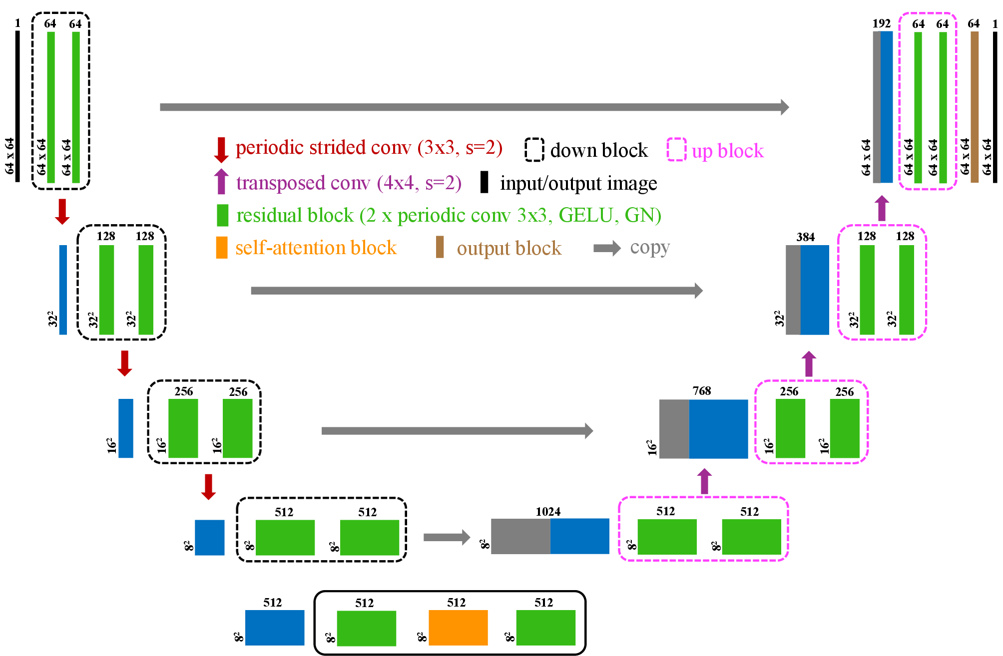
To predict the spatiotemporal evolution of phase separation of a binary mixture, we developed a physics-guided residual U-Net network. The network architecture combines deep residual networks and U-Net architecture while enforcing conservation law through the loss function. The network follows a U-Net–like architecture, consisting of a contracting path, a central bridge, and an expansive path [35]. The contracting path is composed of four downblocks, while the expansive path symmetrically comprises four upblocks. Each downblock and upblock contains two residual blocks, whereas the central bridge is composed of two residual blocks augmented with an attention block. The attention block is placed in the central bridge at the lowest spatial resolution, where the receptive field is at its maximum. At this scale, it efficiently captures global spatial correlations, complementing convolutional features and improving the representation of large-scale morphological evolution. The network architecture is depicted in Fig. 1. Figure 2 depicts the schematic of residual blocks, which consists of two \(3 \times 3\) convolution blocks and identity mapping, or a \(1 \times 1\) convolution with circular padding when the channel dimension differs. The convolution blocks include group normalization (GN), a GeLU activation, and a convolution layer with circular padding.
After each downblock, downsampling is performed using a \(3 \times 3\) convolution with a stride of 2, which reduces the feature map size by half. Further, we double the number of feature channels at each downsampling step. Downsampling is skipped after the final downblock, and its output is directly passed to the central bridge. Correspondingly, in the expansive path, upsampling is performed using transposed convolutions with a kernel size of 4 and a stride of 2 before each upblock. Upsampling increases the spatial resolution by a factor of two while reducing the number of feature channels by half. At each upsampling level, the upsampled features are concatenated with the corresponding skip connections from the contracting path before being processed by the upblocks. After the final upblock, an output layer consisting of a \(3 \times 3\) convolutional layer with circular padding, followed by group normalization (GN) and a GeLU activation, is used to project the multichannel feature map onto the original input space.
2.3 Dataset Generation and Network Training↩︎

We created the dataset by numerically solving the CH equation using a finite-difference method (FDM). For training and validation, we used the system size of \(64 \times 64\), \(\Delta x = 1.0\), \(\Delta t=0.01\). A total of 20 independent trajectories over the interval \(t \in [0, 300]\) are used from critical (\(\psi_0=0\)) and off-critical (\(\psi_0 = -0.4, -0.2, 0.2\), and \(0.4\)) mixtures for training, and five such independent trajectories for validation. For each independent trajectory, we labeled snapshots at any time \(t\) as the input image and corresponding snapshots at time \(t+100\Delta t\) as the target image. Therefore, we used \(59800\) images for training and \(14950\) images for validation. Network performance is tested on ensembles of independent unseen trajectories generated from FDM.
To train the network, we employ a composite loss that balances data fidelity with a physically motivated conservation constraint. Let \(y \in \mathbb{R}^{H \times W}\) denote the ground-truth field and \(\hat{y}\) the network prediction. Here, we use mean-squared error (MSE) \[L_{\mathrm{MSE}} = \left\lVert \hat{y} - y \right\rVert_2^2~,\] to penalize pointwise deviations between predictions and targets. Further, to encode the conservation of the order parameter, which is intrinsic to the underlying conserved dynamics, we introduce an additional penalty term. The spatial mean of each sample is computed as, \[\bar{y} = \frac{1}{HW} \sum_{i,j} y_{ij}~, \qquad \bar{\hat{y}} = \frac{1}{HW} \sum_{i,j} \hat{y}_{ij}~,\] and deviations between predicted and true means are penalized via \[L_{\langle \psi \rangle} = \left( \bar{\hat{y}} - \bar{y} \right)^2.\]
The final training objective is given by \[L = L_{\mathrm{mse}} + \alpha\, L_{\langle \psi \rangle}~, \label{eqn:loss}\tag{13}\] where \(\alpha \geq 0\) controls the strength of the physics-informed regularization. The weights of the network are updated by minimizing the loss function \(L\).
The network is trained using PyTorch Lightning with the AdamW optimizer. We minimized the loss function described in Eq. (13 ) between true and predicted images. It is worth noting that no data augmentation is employed during training. The model is trained using a minibatch size of 16 on an NVIDIA A100 GPU with 40 GB of memory. A fixed learning rate of \(10^{-4}\) is used throughout training, with the physics regularization parameter set to \(\alpha =1.0\). During training, we monitored the loss function and the coefficient of determination (\(R^2\)) to assess convergence and predictive performance. The \(R^2\) score quantifies the fraction of variance in the ground-truth data explained by the model, with values closer to unity indicating better agreement. The parameters/hyperparameters of our network are shown in Table 1.
| Lattice size | \(64\) | |
|---|---|---|
| Number of ensembles | \(20\) | |
| Training samples | \(59800\) | |
| Mixture compositions | \(-0.4\), \(-0.2\), \(0.0\), \(0.2\), \(0.4\) | |
| Time range | \(t \in [0, 300]\) | |
| Training optimizer | AdamW | |
| Learning rate | \(10^{-4}\) |
3 Results and Discussion↩︎
3.1 Training and Validation↩︎
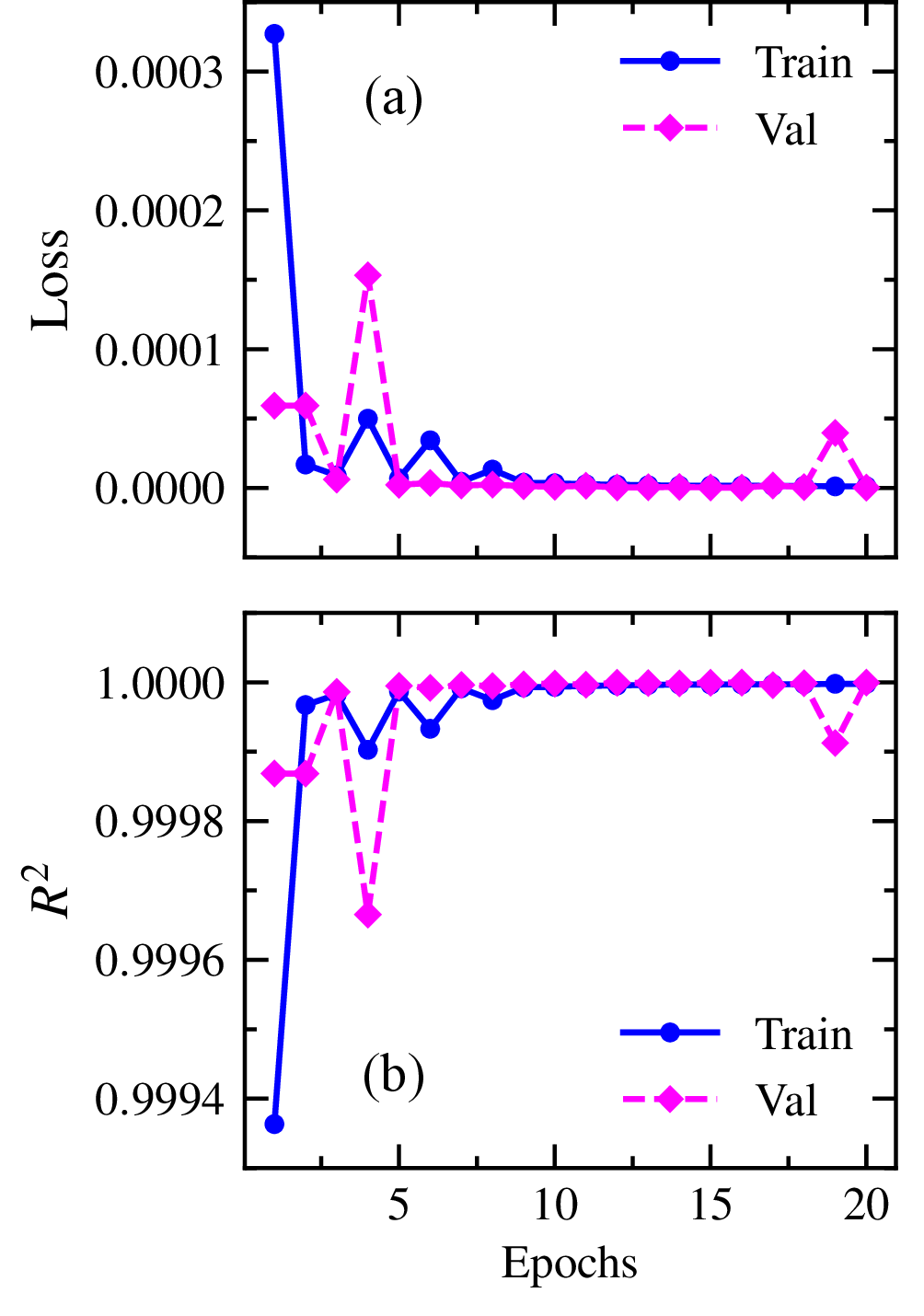
We first present the training and validation performance of the proposed model in Fig. 3. Figure 3 (a) shows the evolution of the loss as a function of training epochs, while Fig. 3 (b) illustrates the corresponding behavior of the coefficient of determination (\(R^2\)). Both metrics exhibit stable convergence, with optimal performance reached at approximately epoch 15 for both training and validation. The model corresponding to this minimum in validation loss is therefore selected for inference, and all results reported in this work are obtained using this checkpoint.
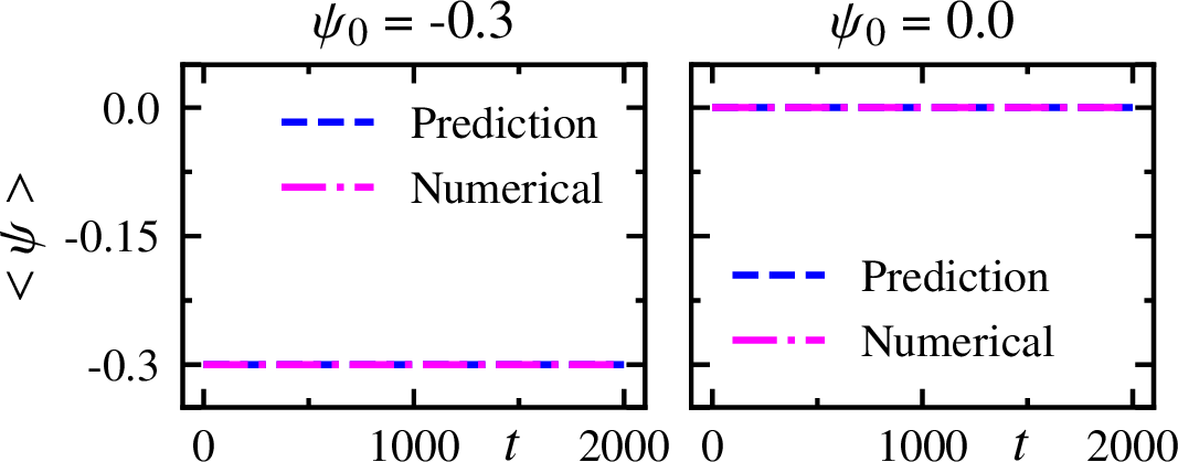
To assess the stability of the model and its ability to preserve the order parameter conservation, we generated 50 independent trajectories each for critical (\(\psi = 0.0\)) and off-critical (\(\psi = -0.3\)) compositions. For each case, the model predicts the full temporal evolution starting from homogeneous initial conditions. The evolution of the spatially averaged order parameter is shown in Fig. 4. As seen, the average composition remains effectively constant over time for both off-critical [see Fig. 4 (a)] and critical [see Fig. 4 (b)] mixtures, demonstrating that the model accurately preserves the global conservation law.
3.2 Domain Morphology in Critical and Off-Critical Mixtures↩︎
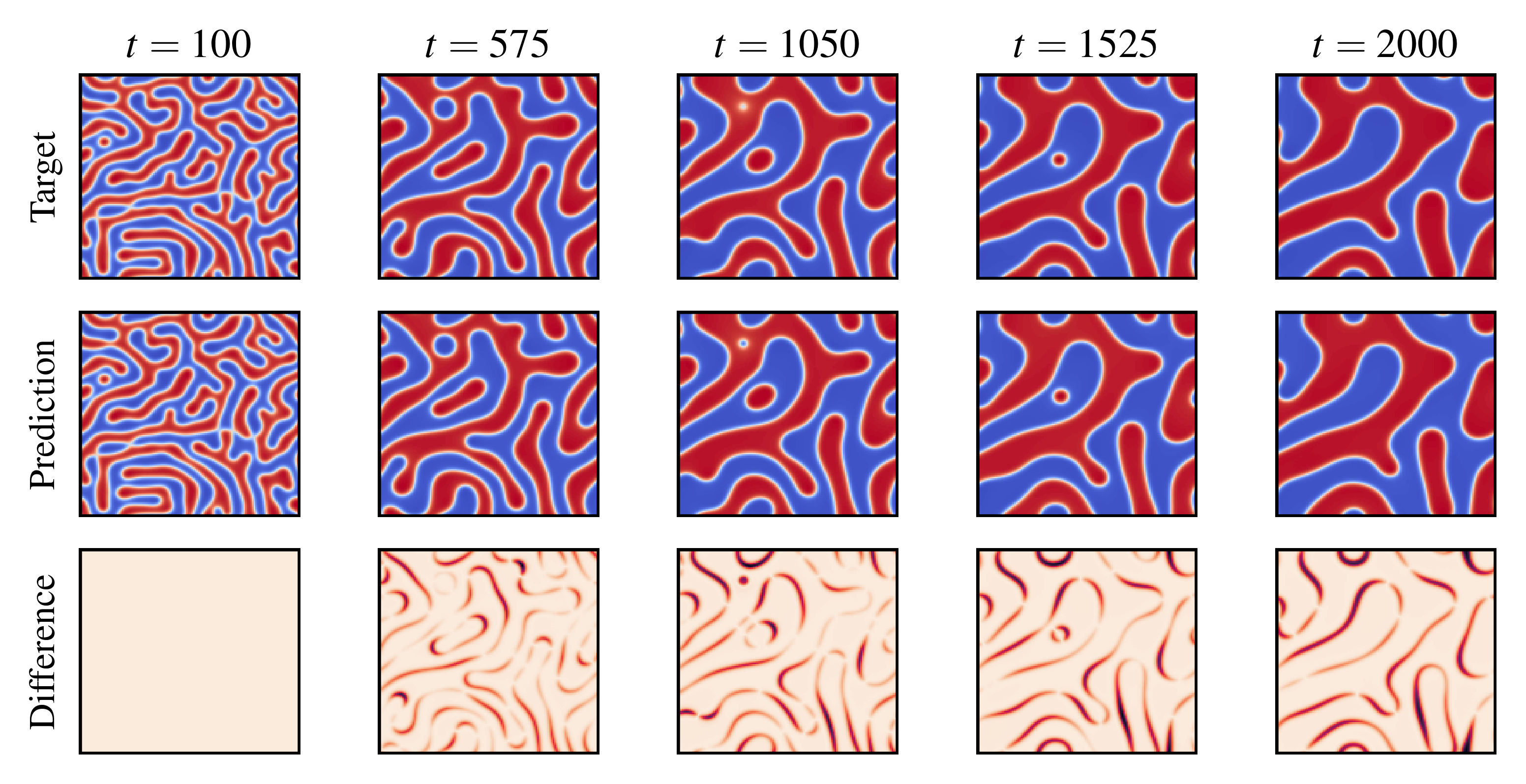
To evaluate the performance of our network architecture, we compare the predicted domain morphologies against numerically generated ground-truth solutions. Figure 5 illustrates the temporal evolution of a binary mixture at critical composition for system size \(128 \times 128\). The top row displays target snapshots obtained via FDM, as discussed in Sec. 2. The middle row shows the network predictions generated autoregressively from the same initial condition as the FDM. Finally, the bottom row highlights the absolute difference between the target and the network predictions. In the visualization, the blue regions correspond to A-rich domains (\(\psi = +1\)), whereas the red regions represent B-rich domains (\(\psi = -1\)). The domain boundaries are represented by the white region where the values of the order parameter are zero. For this analysis, the prediction is initiated at \(t=100\) rather than \(t=0\) to avoid early-time fluctuations, and subsequent snapshots are generated autoregressively. The result presented in Fig. 5 shows good agreement between target and model predictions for a very long time horizon. It is evident that the model captures domain coarsening accurately, while preserving the overall morphology and connectivity of the domains. Furthermore, the analysis of the difference panel reveals that the error made by our proposed framework occurs at domain boundaries and accumulates over the rollout. However, this accumulation remains confined to the interfaces and grows very slowly; therefore, the model remains stable and reliable over long rollouts and can be used for faithful simulation of the CH equation.
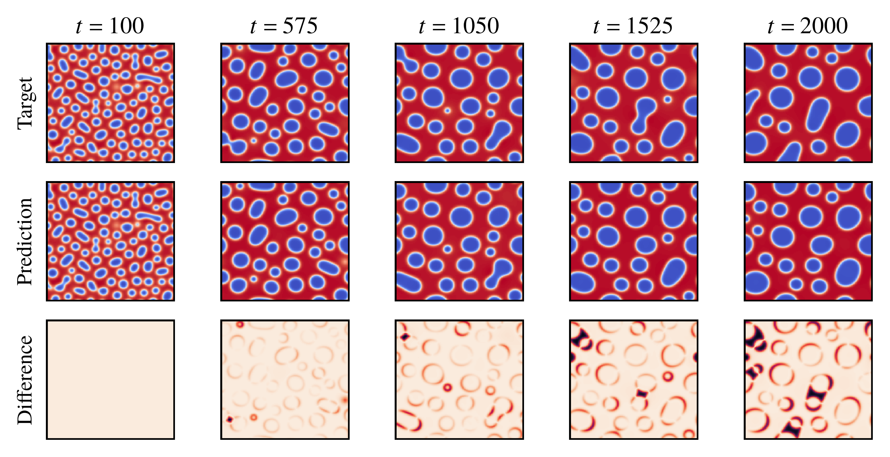
Next, we present the model predictions for off-critical mixtures, as shown in Fig. 6, which depicts the temporal evolution of the domain morphology for a composition of \(\psi = -0.3\). The analysis of snapshots at different times shows that the model accuracy degrades more quickly than observed for the critical mixture. Furthermore, the difference panel of Fig. 6 reveals that the error is no longer confined to the domain boundaries and propagates into the bulk as well. This occurs because the off-critical mixture exhibits a distinct droplet morphology in contrast to the bicontinuous morphology in the critical mixture. These deviations are mainly concentrated in regions undergoing rapid, nonlinear morphological transitions, particularly during active droplet coalescence or breakup events. Nevertheless, the model accurately captures domain coarsening, and the predictions remain stable and reliable over very long time scales.
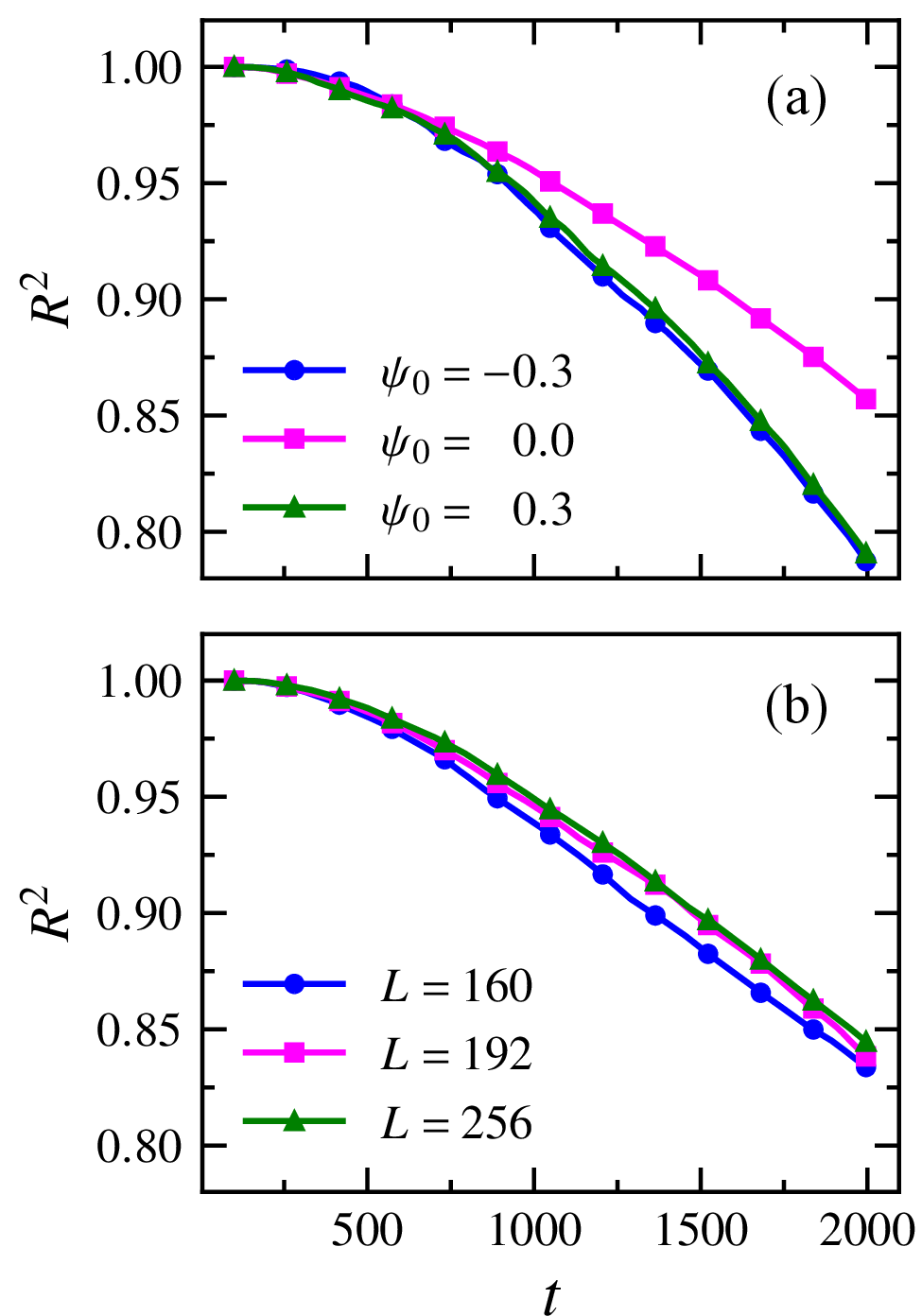
To quantify the morphological observations discussed above, Fig. 7 summarizes the predictive performance of the model across different mixture compositions and system sizes. Figure 7 (a) tracks the temporal evolution of the \(R^2\) for initial compositions (\(\psi_0 = -0.3\), \(0.0\), and \(0.3\)), averaged over \(50\) unseen initial conditions. Consistent with our visual assessments, the model maintains excellent accuracy at early times across all compositions, with \(R^2 \approx 1\). As the simulation progresses, a gradual decay in accuracy emerges due to the natural accumulation of errors inherent in recursive time-stepping; however, the overall predictive performance remains highly robust. Comparing the different compositions, the network exhibits the highest fidelity for the critical mixture (\(\psi_0 = 0.0\)), consistently yielding higher \(R^2\) values throughout the simulation window. In contrast, the off-critical mixtures (\(\psi_0 = \pm 0.3\)) display a slightly accelerated degradation in accuracy over time. This quantitative trend aligns with our earlier morphological analysis, where the droplet morphology in off-critical systems, characterized by localized interface motion, coalescence, and breakup events, leads to sharper gradients and more complex nonlinear dynamics that are more difficult for the model to capture over long trajectories. Further, we evaluated the model performance across different system sizes. We plot \(R^2\) as a function of time for system sizes, \(L = 160\), \(192\), and \(256\) in Figure 7 (b) for the critical composition. It is evident that the model performance remains consistent across all system sizes. This is crucial, as although the model was trained on smaller systems, it can accurately predict larger systems without any noticeable degradation in accuracy.
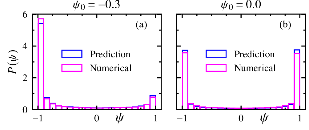
Finally, we examine the distribution of the order parameter to further evaluate the model’s performance. Figure 8 shows the probability distribution \(P(\psi)\) for both off-critical (\(\psi_0 = -0.3\)) and critical (\(\psi_0 = 0.0\)) compositions, comparing the model predictions with numerical results. For the off-critical system as shown in Fig. 8 (a), the distribution is naturally asymmetric, featuring a dominant peak corresponding to the continuous majority phase and a smaller peak representing the dispersed minority phase. The network accurately reproduces this asymmetry, precisely capturing both the locations and relative heights of the phase peaks. While minor deviations are observed near the extreme tails of the distribution (\(\psi \approx \pm 1\)), these are largely attributable to the sharp concentration gradients and finite interface widths inherent to the complex droplet morphology. Conversely, in the critical case as shown Fig. 8 (b), the distribution is perfectly symmetric about \(\psi = 0\), exhibiting pronounced, equal-height peaks near the coexisting bulk phase values (\(\psi \approx \pm 1\)). The predicted distribution closely mirrors the numerical reference, confirming that the model rigorously preserves the physical symmetry of the symmetric mixture and correctly resolves the phase-separated states. Overall, the excellent agreement between the predicted and reference \(P(\psi)\) profiles demonstrates that the neural network framework not only tracks the complex spatial morphology and temporal dynamics, but also faithfully conserves the underlying thermodynamic distribution of the order parameter across the entire system.
3.3 Domain growth in Binary Alloy↩︎
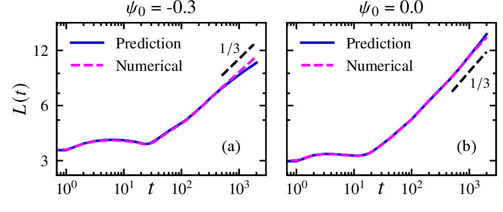
The evolution of the characteristic domain length scale \(L(t)\) during phase separation is shown in Fig. 9 for different mixture compositions. The results obtained from the machine-learning model are compared with those from the numerical solver, along with the expected Lifshitz–Slyozov (LS) growth law for reference. As seen, the predicted growth curves closely follow the numerical results over a wide temporal range for all compositions considered. At early times, the growth of \(L(t)\) is relatively slow due to the presence of strong fluctuations and the initial formation of domains. Despite this, the model accurately captures the initial evolution, indicating that it successfully learns the underlying dynamics even in this highly transient regime. As time progresses, the system enters the coarsening regime, where domains grow steadily, and the agreement between prediction and numerical results remains strong.
For the critical composition (\(\psi_0 = 0.0\)), the agreement is nearly indistinguishable throughout the evolution, demonstrating the model’s ability to capture the dynamics of bicontinuous structures with high fidelity. In the off-critical cases (\(\psi_0 = \pm 0.3\)), a slight deviation between prediction and numerical results emerges at late times, where the predicted growth is marginally slower. This can be attributed to the increased complexity of droplet-based coarsening dynamics, which involve localized interactions such as coalescence and mass transfer between domains. Importantly, the predicted growth behavior remains consistent with the expected LS scaling, as indicated by the dashed reference lines in Fig. 9. This demonstrates that the model not only reproduces the instantaneous morphology but also captures the correct temporal evolution of the characteristic length scale governing the coarsening process.
Having established that the model accurately captures the temporal evolution of the characteristic length scale, we now examine whether it also reproduces the underlying scaling behavior of the system. To this end, we analyze the two-point correlation function \(C(r,t)\) at different times by rescaling the spatial coordinate with the characteristic domain size \(L(t)\). Figure 10 shows the scaled correlation function \(C(r,t)\) plotted as a function of the reduced distance \(r/L(t)\) for different times. For all compositions, the curves corresponding to different time instants collapse onto a single master curve, demonstrating the emergence of dynamical scaling during the coarsening process. This collapse indicates that the evolving domain morphology is statistically self-similar, with the characteristic length scale \(L(t)\) serving as the only relevant length scale governing the structure of the system. The quality of the collapse remains consistent across both off-critical and critical compositions, as seen in Figs. 10 (a) and (b), respectively. Minor deviations are observed at larger values of \(r/L\), where statistical fluctuations become more pronounced, particularly for off-critical mixtures. Nevertheless, the overall agreement confirms that the model successfully captures not only the growth kinetics but also the correct spatial correlations underlying the phase separation process.
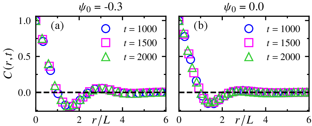
These results, together with the agreement in \(L(t)\), demonstrate that the proposed framework accurately reproduces the essential physical features of phase separation, including domain growth and dynamical scaling, over extended time evolution.
4 Conclusions↩︎
We developed an attention-based, physics-guided convolutional neural network to predict the domain growth in systems with conserved kinetics. The proposed framework is trained to capture domain coarsening in binary mixtures, where, following a sudden quench, the system evolves through the formation and subsequent growth of domains. In such systems, the overall composition remains conserved throughout the evolution, and to achieve this, we explicitly incorporated the conservation law into the loss function.
Furthermore, the use of residual blocks enables the effective training of deeper networks. Additionally, attention mechanisms are incorporated at the lowest resolution to balance computational efficiency while accurately capturing long-range spatial correlations. The model is trained on early-time evolution snapshots for a system size of \(64 \times 64\), with the objective of predicting a single snapshot at a time \(100\Delta t\) ahead. The full spatiotemporal evolution is then generated by recursively feeding the model outputs back as inputs.
In this work, we evaluate the model performance when predictions are initiated from both late-time snapshots and random initial configurations. Predictions starting from late-time states show better one-to-one correspondence with the ground truth, whereas those initiated from random configurations deviate at long times. Notably, even in the absence of a strict one-to-one agreement, the model still captures the correct statistical and dynamical behavior. This is reflected in the accurate domain growth law obtained from the evolution of the characteristic length scale, which shows excellent agreement with the Lifshitz–Slyozov growth law \(L(t) \sim t^{1/3}\), as well as the preservation of dynamical scaling, evidenced by the collapse of the correlation function \(C(r, t)\) when plotted against the rescaled distance \(r/L(t)\).
Finally, the model accurately learns the system dynamics while preserving the underlying conservation laws, enabling its extension beyond this prototypical problem to a broader class of systems with conserved kinetics. However, this requires prior knowledge of the conservation law, as it is explicitly encoded in the loss function. A promising direction for future work is to enable the model to learn such conservation laws directly during training.
ACKNOWLEDGEMENTS↩︎
P.K.J. acknowledges the financial support from the Science and Engineering Research Board (SERB), Department of Science and Technology (DST), India (Grant Nos. CRG/2022/006365 and ITS/2024/001866) and IIT Jodhpur for a Seed Grant (No. I/SEED/PKJ/20220016).
CONFLICT OF INTEREST↩︎
All authors declare they have no competing interests.
References↩︎