1 Introduction↩︎

Efficient numerical integration is a key challenge in many disciplines, including data science, physics, engineering, and Bayesian statistics, where high-dimensional integrals arise in tasks such as model selection [1], [2], parameter estimation and uncertainty quantification [3]–[8], and partition function evaluation [9]–[13]. While classical quadrature methods quickly become intractable in high dimensions, stochastic methods such as Monte Carlo integration, importance sampling [14]–[17], and Nested Sampling [18], [19] have proven effective when the integrand is inexpensive to evaluate.

In many scientific and engineering applications, however, evaluating the target function is computationally expensive. A single evaluation may require a large-scale simulation, the solution of a complex physical model, or the processing of high-resolution data [5], [7], [10]. In such settings, standard integration methods can become inefficient because they require many target evaluations. At the same time, low-fidelity approximations or surrogate models are often available and capture useful structure of the integrand at substantially lower cost. These approximations may take the form of coarse physical models [7], [8], simplified energy landscapes [10], [12], or machine-learned regressors trained on high-fidelity data [20]–[24]. The central challenge is to use such approximations to guide integration, accelerate computation, and reduce variance without introducing bias.

Several approaches have been proposed to address this challenge. Sequential Monte Carlo methods construct a sequence of weighted particle approximations to the target distribution, often combining reweighting, resampling, and mutation steps to balance bias and variance [25], [26]. Multifidelity Monte Carlo and Multilevel Monte Carlo methods combine simulations at different fidelities using control variates or telescoping estimators to reduce variance while maintaining unbiasedness [27]–[29]. Adaptive importance sampling techniques construct proposal distributions informed by surrogate models or auxiliary densities to concentrate samples in high-contribution regions [14], [30]. Stratified sampling methods reduce variance by partitioning the parameter space into regions of approximately equal weight. However, standard stratification often relies on simple strata, such as axis-aligned partitions [15], which may poorly reflect complex posterior geometries. While these methods can perform well for expectation estimation, they often struggle to scale efficiently to high-dimensional or multimodal distributions, and typically do not yield posterior samples without additional approximation or resampling techniques [31], [32].

In contrast, Nested Sampling provides a framework for estimating Bayesian evidence and generating posterior samples simultaneously [18], [19]. By constructing nested likelihood contours and estimating the associated constrained prior masses, it enables efficient exploration of complicated multimodal distributions. Recent extensions incorporate dynamic allocation of samples [33], [34], slice-sampling-based exploration of the constrained prior in high dimensions [35], or adaptations for multimodality [32], [36], [37], but they still rely on target evaluations to estimate constrained prior masses. Moreover, reweighting schemes based on Nested Sampling still require many target evaluations, because the fidelity of the volume estimate remains directly tied to the number of target function calls, as we discuss in Section 2.3.

In this paper, we introduce Slice Monte Carlo integration (S\(\ell\)MC), a method that combines the strengths of stratified Monte Carlo and Nested Sampling for surrogate-based integration. S\(\ell\)MC applies a Nested Sampling-like procedure to the surrogate to partition the space into informative strata, or slices, while generating prior samples within each slice. This enables stratified Monte Carlo integration over the surrogate-induced partition and yields efficient estimates of the target integral. A key advantage over standard reweighting techniques is that volume estimation is decoupled from target function evaluation. Slice volumes can therefore be estimated accurately using the cheap surrogate, while expensive target evaluations are allocated adaptively across slices. Furthermore, the surrogate-induced partition facilitates efficient generation of posterior samples via rejection sampling.

The term slice in this paper denotes surrogate-induced strata for integration. This differs from Neal’s slice sampling for Markov chain Monte Carlo [38], and from the use of slice sampling as a constrained-prior sampler in NS implementations such as PolyChord [35].

The remainder of this paper is structured as follows. In Section 2, we formalize the problem setup and review stochastic integration methods relevant to the development of S\(\ell\)MC. Section 3 introduces the slicing framework, followed by a detailed presentation of the S\(\ell\)MC algorithm, including its theoretical properties, such as unbiasedness and variance, and a discussion on generating posterior samples. Finally, Section 4 demonstrates the performance of the proposed method on benchmark problems.

2 Problem Setup and Related Methods↩︎

We are interested in evaluating integrals of the form \[\label{eq:evidence} \mathcal{Z} = \mathbb{E}_\pi[L] = \int_{\Omega} L(\theta)\;\mathrm{d}\pi(\theta)\,,\tag{1}\] over a Borel-measurable parameter space \(\Omega \subset \mathbb{R}^d\) for \(d \geq 1\), where \(L: \Omega \rightarrow \mathbb{R}\) is the target function and \(\pi\) is a prior probability distribution on \(\Omega\). Specifically, this includes evidence integrals in the context of Bayesian inference, where \(L\) is the non-negative likelihood function or partition function in statistical physics, e.g., the non-negative exponential Boltzmann factor. This integral is particularly demanding because the prior probability distribution function \(\pi(\theta)\) typically has a much smaller variability than the target function \(L(\theta)\).

Another goal of this paper is based on the posterior distribution \(\mathrm{d}p(\theta) = L(\theta)\,\mathrm{d}\pi(\theta) / \mathcal{Z}\), for which either the generation of uncorrelated samples or posterior expectation values of the form \[\label{eq:expectation} \mathcal{G} = \mathbb{E}_{p}[g] = \int_{\Omega} \; g(\theta)\;\mathrm{d} p(\theta)\,.\tag{2}\] are of great interest. This type of problem arises in many contexts, including statistical inference, uncertainty quantification, and statistical physics, where, e.g., the posterior expectation corresponds to the thermodynamic expectation of some physical observable.

To estimate such integrals and obtain samples, various stochastic integration techniques have been developed. Below, we briefly review the most relevant integration approaches that form the conceptual foundation for Slice Monte Carlo integration (S\(\ell\)MC) proposed in the present paper.

2.1 Monte Carlo Integration↩︎

In standard Monte Carlo integration (simple sampling), expectations with respect to \(\pi\) are estimated using the empirical mean over independent and identically distributed samples \(\Theta_1, \dots, \Theta_N \overset{\mathrm{iid}}{\sim} \pi\). For the evidence integral \(\mathcal{Z} = \mathbb{E}_{\pi}[L]\), this yields the estimator \[\label{eq:MC32Z} \widehat{\mathcal{Z}}_N^\text{MC} = \frac{1}{N}\sum_{i=1}^N L(\Theta_i)\,,\tag{3}\] which is unbiased, converges at rate \(\mathcal{O}(N^{-1/2})\) and is asymptotically normal provided that \(\mathrm{\mathbb{V}ar}_{\pi}[L] < \infty\).[16] Its variance is given by \[\label{eq:MC32var32Z} \mathrm{\mathbb{V}ar}[\widehat{\mathcal{Z}}_N^\text{MC}] = \frac{1}{N} \mathrm{\mathbb{V}ar}_{\pi}[L]\,.\tag{4}\]

2.1.1 Monte Carlo Importance Sampling↩︎

Simple sampling may be inefficient when significant contributions to \(\mathcal{Z}\) come from regions of low probability under \(\pi\). If a nonnegative surrogate function \(\phi(\theta)\) can be found for which the integral \(\mathcal{Z}_\phi = \mathbb{E}_{\pi}[\phi]\) is known, or can easily be evaluated to arbitrary precision, then one can introduce a new probability measure \(\mathrm{d}p_\phi(\theta) = \phi(\theta)\,\mathrm{d}\pi(\theta) / \mathcal{Z}_\phi\) and the target integral \(\mathcal{Z}\) can be written as \[\label{eq:IS32int95new} \mathcal{Z} = \mathcal{Z}_\phi \;\mathbb{E}_{p_\phi}[L / \phi]\,.\tag{5}\]

The resulting Monte Carlo estimator, which we refer to as importance sampling (IS) estimator, remains unbiased and has variance \[\label{eq:IS32var32Z} \mathrm{\mathbb{V}ar}[\widehat{\mathcal{Z}}_N^\text{IS}] = \frac{\mathcal{Z}_\phi^2}{N} \mathrm{\mathbb{V}ar}_{p_\phi}[L / \phi]\,.\tag{6}\] Crucially, \(\mathcal{Z}_\phi\) must be known, which in itself can be a complicated task. If the surrogate \(\phi(\theta)\) resembles closely the target function \(L(\theta)\) then the numerical effort to compute \(\mathcal{Z}_\phi\) is the same as the numerical effort to compute \(\mathcal{Z}\), unless it allows an analytical evaluation, or to use more efficient numerical techniques which are not applicable to \(L(\theta)\). Moreover, the choice of \(\phi\) strongly influences efficiency. A mismatch between \(\phi\) and \(L\) can lead to a large variance of the estimator. Adaptive schemes that iteratively construct surrogates, e.g. product approximations \(\phi(\theta) = \prod_{j=1}^d g_j(\theta_j)\), have been proposed [14], [17], but typically rely on independence assumptions across dimensions.

2.1.2 Stratified Monte Carlo Integration↩︎

Stratification can also reduce the variance of the integrand. To that purpose, \(\Omega\) is partitioned into disjoint regions (strata) \(\mathscr{S}_1, \dots, \mathscr{S}_{M}\), with \(\Omega = \cup_{i=1}^M \mathscr{S}_{i}\), and the integral can be written as \[\mathcal{Z} = \sum_{i=1}^{M} \int_{\mathscr{S}_i} L(\theta)\;\mathrm{d}\pi(\theta)\,.\] Each term is then estimated separately via Monte Carlo \[\widehat{\mathcal{Z}}_\mathscr{S} = \sum_{i=1}^{M} \frac{S_i}{N_i} \sum_{k=1}^{N_i} L(\Theta_{i,k})\,,\] where \(S_i = \pi[\mathscr{S}_i]\) is the prior mass of stratum \(\mathscr{S}_i\), and \(\Theta_{i,k} \overset{iid}{\sim}\pi|_{\mathscr{S}_i}\) for \(i = 1,\ldots, M\) and \(k = 1, \ldots, N_i\).

Sample allocation can be optimized to minimize the total variance. Writing \(N = \sum_{i=1}^M N_i\), the optimal allocation is [15] \[\label{eq:MC32strat32number32of32sample32points} \frac{N_i}{N} = \frac{S_i \sigma_{\mathscr{S}_i}}{ \sum_{k=1}^M S_k \sigma_{\mathscr{S}_k}}\,,\tag{7}\] where \(\sigma^2_{\mathscr{S}_i} = \mathrm{\mathbb{V}ar}_\pi[L(\Theta) \vert \Theta\!\in\!\mathscr{S}_i]\) denotes the variance of \(L\) in stratum \(\mathscr{S}_i\). So the minimal variance, if only the number of points per stratum \(N_1, \ldots, N_M\) are optimized, reads \[\require{physics} \mathrm{\mathbb{V}ar}_{\text{opt}}[\widehat{\mathcal{Z}}_\mathscr{S}] = \frac{1}{N} \qty(\sum_{i=1}^M S_i \sigma_{\mathscr{S}_i})^{\!\!2}\] as compared to \[\mathrm{\mathbb{V}ar}_{\text{eq}}[\widehat{\mathcal{Z}}_\mathscr{S}] = \frac{M}{N} \sum_{i=1}^M S^2_i \sigma_{\mathscr{S}_i}^2\] if the same number \(N_i = N/M\) is used in all strata. The difference \[\begin{align} \mathrm{\mathbb{V}ar}_{\text{eq}}[\widehat{\mathcal{Z}}_\mathscr{S}] - \mathrm{\mathbb{V}ar}_{\text{opt}}[\widehat{\mathcal{Z}}_\mathscr{S}] &= \frac{M}{N} \bigg( \sum_{i=1}^M \big[S_i \sigma_{\mathscr{S}_i} - \overline{S\sigma }\big]^2\bigg) > 0\;,\quad \text{with } \overline{S\sigma} := \frac{1}{M} \sum_{i=1}^M S_i \sigma_{\mathscr{S}_i} \end{align}\]

Despite its potential, stratification poses two key challenges: identifying effective strata a priori is nontrivial in high dimensions, and sampling from the prior within each stratum may be difficult and computationally expensive. Common approaches use axis-aligned partitions or recursive bisection along directions of high variance [15], [17]. Adaptive stratification can improve performance, but a large number of evaluations may still be needed. Additionally, simple bisections of dimensions can violate symmetries of the integrand and therefore reduce the efficiency. This limitation is addressed in S\(\ell\)MC, where we design informative strata that are adapted to the target function, via a Nested Sampling-like procedure applied to a surrogate.

2.2 Nested Sampling↩︎

2.2.1 Rewriting the Evidence Integral↩︎

Before introducing S\(\ell\)MC, we briefly review the principles of Nested Sampling (NS). NS begins by reformulating the evidence integral in Equation 1 over a positive likelihood function \(L:\Omega\to\mathbb{R}_{>0}\) as an integral over the constrained prior mass \(X(\lambda) := \pi[L(\Theta) > \lambda]\) \[\mathcal{Z} = \int_0^1 \widetilde{L}(x)\;\mathrm{d}x\,,\] where \[\widetilde{L}(x) = \sup\{\lambda\in\mathbb{R} \,\vert\, X(\lambda) > x\}\] is the generalized inverse of \(X\), also interpreted as the likelihood corresponding to the contour enclosing prior mass \(x\) [18], [19], [39]–[41].

This transforms the high-dimensional integral into a one-dimensional integral over the unit interval, which can then be approximated using standard quadrature \[\label{eq:NS32estimator} \mathcal{Z} \approx Z = \sum_{i=1}^K w_i \widetilde{L}_i\,,\tag{8}\] where \(w_i = X_{i-1} - X_i\) are weights associated with prior mass differences and \(\widetilde{L}_i\) are corresponding likelihood values.

Since \(\widetilde{L}(x)\) is a monotonically decreasing function in the constrained prior mass \(x\), Equation 8 yields an upper bound for the true \(\mathcal{Z}\), while \(\sum_{i=1}^K w_i \widetilde{L}_{i-1}\) is a strict lower bound. However, evaluating \(X(\lambda)\) exactly is intractable, and it must be approximated stochastically.[18], [19]

2.2.2 The Nested Sampling Procedure↩︎

NS estimates \(X\) by random sampling from level sets of increasing likelihood. The key identity is that for \(\Theta \sim \pi|_{>L^*}\), i.e. drawn from the prior constrained to the set \(\{L > L^*\}\), \(X(L(\Theta)) \sim \mathrm{Uniform}(0, X^*)\), where \(X^* = X(L^*)\). This identity holds if \(X\) is continuous, which is the case if \(L\) has no plateaus of non-zero probability with respect to \(\pi\). [40], [41]

By drawing \(N_{\mathrm{live}}\) independent samples from \(\pi\vert_{>L^*}\) and sorting them by likelihood, \[\label{eq:ordered32sample} \begin{array}{ccccccc} L_{(1)} &>& L_{(2)} &>& \cdots &>& L_{(N_{\mathrm{live}})} \\ X_{(1)} &<& X_{(2)} &<& \cdots &<& X_{(N_{\mathrm{live}})}\,, \end{array}\tag{9}\] the smallest likelihood corresponds to a prior mass \(X_{(N_{\mathrm{live}})} = t X^*\) where \(t \sim \mathrm{Beta}(N_{\mathrm{live}},1)\), as given by the maximum statistics.[19], [39] The number \(N_{\mathrm{live}}\) is typically referred to as the number of live points.

This procedure can be used to compress the prior mass iteratively, via the recursion \[X_i = t_i X_{i-1}, \quad \text{with } t_i \sim \mathrm{Beta}(N_{\mathrm{live}},1), \quad X_0 = 1\,,\] The contraction factors \(t_i\) are mutually independent, as they are associated with independent uniform samples from the constrained prior. Conditional on the sampled likelihood values \(\{\widetilde{L}_i\}\), the quadrature estimate is therefore a function of the compression factors, and we write \(Z=Z(\boldsymbol{t})\) to indicate this dependence, where \(\boldsymbol{t} = (t_1, \dots, t_K)\) denotes the vector of compression factors.

At each step, the live point with the lowest likelihood is discarded and stored, and a new point is drawn from the new constrained prior \(\pi\vert_{>L_i}\). In practice the constrained draw is the dominant cost of NS, and a variety of constrained samplers have been proposed, ranging from standard Markov chain Monte Carlo methods [19] and ellipsoidal rejection [32] to slice-sampling chains [35]. The other live points already fulfill the constraint by construction. Repeating this for \(K\) steps yields a sequence \(\{\theta_i, \widetilde{L}_i, X_i(\boldsymbol{t})\}\) which forms the quadrature rule in Equation 8 . The use of the maximum statistic in each iteration is optimal in nested sampling, as it minimizes the estimator variance and maximizes the resolution of the quadrature.[19] While alternative order statistics are theoretically possible, they generally lead to inferior performance. To ensure that the quadrature adequately captures the bulk of the posterior mass, the number of iterations should satisfy \(K\geq N_{\mathrm{live}}H\), where \(H\) is the relative entropy (or Kullback–Leibler divergence) from the posterior to the prior.[19] This condition ensures that the nested sampling trajectory penetrates deeply enough into high-likelihood regions to estimate both the evidence and the posterior accurately.

Dynamic nested sampling methods [33], [34] extend this framework by adaptively varying the number of points and termination criteria during sampling to enhance efficiency, particularly in the estimation of posterior expectations.

2.2.3 Error analysis↩︎

NS in this form produces not only a point estimate but a distribution over evidence estimates \(Z(\boldsymbol{t})\), conditional on the sampled likelihood values, which we indicate by conditioning on \(\boldsymbol{\theta}\). The remaining uncertainty in \(Z(\boldsymbol{t})\) then comes from the stochastic compression factors \(\boldsymbol{t}\). The compression factors may be set deterministically, e.g., \(t_i = \exp(-1/N_{\mathrm{live}})\) or \(t_i = N_{\mathrm{live}}/(N_{\mathrm{live}}+1)\), or sampled from \(\mathrm{Beta}(N_{\mathrm{live}},1)\).[19], [39], [42]–[44]

From now on, we assume that \(t_1, \ldots, t_K\) are iid with \(t_1 \sim \mathrm{Beta}(N_{\mathrm{live}},1)\). Error analysis can be conducted either using information-theoretic arguments [19], or through a moment-based analysis [39], [42]. The latter approach yields formulas for the expectation and variance of \(Z(\boldsymbol{t})\), given the knowledge of all sampled points during the procedure. Exploiting the independence of the compression factors \(t_i\) and using \(\mathbb{E}[t_i] = N_{\mathrm{live}}/(N_{\mathrm{live}}+1)\), one obtains \[\require{physics} \mathbb{E}[Z\vert\boldsymbol{\theta}]\! =\! \sum_{i=1}^K \mathbb{E}[w_i\vert\boldsymbol{\theta}]\, \widetilde{L}_i = \frac{1}{N_{\mathrm{live}}}\!\sum_{i=1}^K \! \!\qty(\frac{N_{\mathrm{live}}}{N_{\mathrm{live}}+1})^{\!\!i} \widetilde{L}_i\,.\] In practical applications, it is often sufficient to consider the distribution \(Z(\boldsymbol{t})\) given the observed data, whose uncertainty arises from the stochastic nature of NS. Taking its conditional expectation yields a Bayesian point estimator of the evidence. It can be shown that this point estimator is asymptotically unbiased and asymptotically normally distributed under additional regularity conditions.[45] Note, however, that the remaining randomness of the point estimator is contained in \(\widetilde{L}_i\), which are obtained by the sorting procedure, and therefore, a simple error analysis of the point estimator is not applicable. Nevertheless, reformulations in terms of sequential Monte Carlo algorithms exist, which provide an inherently unbiased estimator for Nested Sampling.[25] For high-dimensional integrals, Skilling pointed out that instead of \(Z\) the relevant quantity is \(\log(Z)\), which is usually closer to a normal distribution.[39], [46]

For the conditional variance, [39], [42] provide an explicit expression when the number of live points is constant. Here we will only investigate the general structure of the variance, to analyze the sources of uncertainty, \[\begin{align} \begin{aligned} \mathrm{\mathbb{V}ar}[Z\vert\boldsymbol{\theta}] &= \mathrm{\mathbb{V}ar}[\sum_{i=1}^K w_i \widetilde{L}_i\vert\boldsymbol{\theta}]= \sum_{i=1}^K \widetilde{L}_i^2 \mathrm{\mathbb{V}ar}[w_i\vert\boldsymbol{\theta}] + 2\!\sum_{\substack{i,j =1 \\ i<j}}^K\! \widetilde{L}_i \widetilde{L}_j \mathrm{\mathbb{C}ov}[w_i,w_j\vert\boldsymbol{\theta}]\,. \end{aligned} \end{align}\] Using the decomposition \(w_j = X_i \prod_{k=i+1}^{j-1} t_k\; (1-t_j)\) and the independence of the compression factors, we get \[\begin{align} \label{eq:NS32var} \begin{aligned} \mathrm{\mathbb{V}ar}[Z\vert\boldsymbol{\theta}] =\sum_{i=1}^K\!\Bigg(\widetilde{L}_i^2& \mathrm{\mathbb{V}ar}[w_i\vert \boldsymbol{\theta}] + 2\widetilde{L}_i \mathrm{\mathbb{C}ov}[w_i,X_i\vert\boldsymbol{\theta}]\!\sum_{j=i+1}^K\!\! \Big(\widetilde{L}_j \mathbb{E}[1\!-\!t_j]\prod_{k=i+1}^{j-1}\!\!\!\mathbb{E}[t_k] \Big) \Bigg)\,. \end{aligned} \end{align}\tag{10}\] We will see in Section 3.2, why this particular decomposition of the variance of NS allows for an easy interpretation of the variance terms present in S\(\ell\)MC. Further details can also be found in [39], where it is also shown that for a large number of live points \(N_{\mathrm{live}}\), the variance of \(Z\) is \(\order{1/N_{\mathrm{live}}}\) like in standard MC. This implies that increasing the number of live points reduces the uncertainty, but at a price: The mean compression factor for large \(N_{\mathrm{live}}\) is \(t \approx e^{-1/N_{\mathrm{live}}}\), hence the mean prior mass at step \(i\) is \(X_i \approx e^{-i/N_{\mathrm{live}}}\). In realistic problems, the dominant part of the likelihood corresponds to a very small prior mass \(X^*\), which has to be reached for convergence. The number of necessary steps \(m^*\) follows from \(X_{m^*} = X^*\) and gives \(m^* = N_{\mathrm{live}} \left\lvert{\ln(X^*)}\right\rvert\). Hence, the number of steps and therefore the number of function evaluations increases proportionally to \(N_{\mathrm{live}}\) and in turn inversely proportional to \(\varepsilon_Z^2\), the desired relative uncertainty. We see, the stochastic uncertainty in NS comes entirely from the constrained prior masses, which are determined by \(N_{\mathrm{live}}\). We will see later that it is possible to determine the thresholds differently and obtain a way to strongly reduce the uncertainty of the constrained prior masses by adding uncertainty to the likelihood values, which allows for more flexibility to optimize the algorithm.

2.2.4 Posterior Representatives↩︎

NS can also be used to generate posterior representatives. Since the weighted likelihood values \(\widetilde{L}_i\) are associated with constrained prior masses \(X_i\), one can assign normalized weights \[p_i(\boldsymbol{t}) = w_i(\boldsymbol{t}) \widetilde{L}_i / Z(\boldsymbol{t})\] to obtain a discrete approximation of the posterior distribution \(\mathrm{d}p(\theta) \!\!=\! L(\theta)\,\mathrm{d}\pi(\theta) / \!\mathcal{Z}\). This still contains the uncertainty of the compression factors \(\boldsymbol{t}\). The probability \(\hat{p}_i\) for \(\theta_i\) is now given by the mean \(\mathbb{E}_{\boldsymbol{t}}[w_i(\boldsymbol{t}) \widetilde{L}_i / Z(\boldsymbol{t})]\), which is easily obtained by MC means. This can be used to estimate the expectation \(\mathcal{G} := \mathbb{E}_{p}[g]\) of an \(p\)-integrable quantity \(g:\Omega\to\mathbb{R}\) by \[G(\boldsymbol{t}) = \sum_{i=1}^K p_i(\boldsymbol{t}) g(\theta_i)\] or to obtain an equally weighted posterior sample by accepting each \(\theta_i\) with probability \(\hat{p}_i / C\), with \(C \geq \max_i \hat{p}_i\).[19]

Similarly, a sampling-based or moment-based error analysis is also possible in this case. However, it is unclear whether \(g(\theta_i)\) is indeed a good representative of the function \(g\) within the volume associated with the weight \(w_i\).[44]

2.3 Reweighting↩︎

Similar to importance sampling, the NS procedure can be reused to estimate the integral of a target function \(L\) using a surrogate model \(\phi\).[45], [47], [48] Specifically, if samples \(\theta_i^{\phi}\) are drawn using NS applied to \(\phi\), we can express the evidence \(Z\) for \(L\) as the expectation in Equation 5 , yielding \[\label{eq:Z} Z(\boldsymbol{t}_\phi) = \sum_{i=1}^K p_{\phi,i}(\boldsymbol{t}_\phi)\, Z_\phi(\boldsymbol{t}_\phi) \, L(\theta_{\phi,i}) / \widetilde{\phi}_i = \sum_{i=1}^K w_{\phi,i}(\boldsymbol{t}_\phi) \, L(\theta_{\phi,i})\,,\tag{11}\] where \(p_{\phi,i} = w_{\phi,i} \widetilde{\phi}_i / Z_\phi\) are posterior representatives of the surrogate model, and \(w_{\phi,i}\) the volume elements derived from the surrogate model. As a matter of fact, \(w_{\phi,i}(\boldsymbol{t}_\phi)\) is independent of the likelihood and it therefore has the same PDF as \(w_i(\boldsymbol{t})\). The estimator in Equation 11 is analogous to that of standard NS for \(Z\), but here \(L\) is evaluated at the sampled points \(\theta_{\phi,i}\) obtained by NS based on \(\phi\).

The surrogate-based quadrature inherits the volume uncertainty of NS applied to \(\phi\). In addition, if \(\phi\) and \(L\) do not induce the same ordering, the value \(L(\theta_{\phi,i})\) may be a poor representative of the target function over the prior-mass element \(w_{\phi,i}\), which introduces an additional source of variance.

At first glance, Equation 11 looks like there is nothing gained by using the surrogate. One important advantage, however, is the fact that the generation of constrained prior points, which typically necessitates several likelihood evaluations [19], [35], is done with the low-cost surrogate. And that is, as we will see in the results section, a huge advantage if the true likelihood is expensive.

A key advantage of reweighting over classical importance sampling is that it becomes NS when \(L\) and \(\phi\) induce the same ordering over \(\Omega\), i.e. if \(L(\theta_1) < L(\theta_2)\) is equivalent to \(\phi(\theta_1) < \phi(\theta_2)\) for all \(\theta_1, \theta_2 \in \Omega.\) In this case, the nested samples \(\theta_{\phi,i}\) and associated volumes \(w_{\phi,i}\) exactly match those that would have been produced by applying NS directly to \(L\), and the reweighted estimator reproduces the NS result.

As in standard NS, the stochasticity lies in the volume elements \(w_{\phi,i}\), so moment-based error analysis [42] still applies. However, a new source of error arises, as \(L\) may vary significantly within the region associated with \(w_{\phi,i}\), making \(L(\theta_{\phi,i})\) a potentially poor representative of that volume. Additionally, the number of point evaluations of \(L\) must match the number of estimated volumes \(w_{\phi,i}\), tying computational cost to quadrature resolution. Both issues are directly addressed by S\(\ell\)MC, which decouples volume estimation from point evaluations for the target function and allows for adaptive sampling within each slice.

3 Slicing and Slice Monte Carlo↩︎

3.1 Slicing – Partitioning of the Parameter Space↩︎

With these prerequisites in place, we now introduce the partitioning of the parameter space into slices and the corresponding slice Monte Carlo integration (S\(\ell\)MC), which combines ideas of Nested Sampling, reweighting, and stratified Monte Carlo. By using a positive function \(\phi:\Omega\to\mathbb{R}_{>0}\), which can be chosen as a cheap surrogate for the target function \(L\), the core idea is to construct a sequence of thresholds \(\{\phi_i\}_{i=0}^{M-1}\), with \(\phi_0 = 0\), using a Nested Sampling-like procedure. These thresholds define level sets \[\mathscr{X}_i := \{\theta\in\Omega\,\vert\, \phi(\theta) > \phi_i\}\,,\quad X_i := \pi[\mathscr{X}_i]\,,\quad i=0,\dots,M-1\,.\] where \(X_i\) is the constrained prior mass above \(\phi_i\). For notational convenience, we set \(\mathscr{X}_M=\emptyset\) and \(X_M=0\). This induces a partition of the parameter space into slices \[(\mathscr{S}_i, S_i) = (\mathscr{X}_{i-1} \setminus \mathscr{X}_i,\; X_{i-1} - X_i)\,,\quad i=1,\dots,M\,,\] where \(S_i = \pi[\mathscr{S}_i]\) is the prior mass in slice \(\mathscr{S}_i\). After constructing the slices, we can use samples drawn from the constrained prior within each slice \(\mathscr{S}_i\) to compute the target integral via stratified Monte Carlo integration.

Constrained sampling within each slice is generally very demanding, due to two constraints – upper and lower – on the value of the slicing function \(\phi\). However, the Nested Sampling-like procedure, where only the lower constraint is used to construct the slices, can also be used to generate the necessary samples.

In each iteration \(i=1,\dots,M-1\) a new threshold \(\phi_i > \phi_{i-1}\) is chosen. It may be chosen arbitrarily, prescribed in advance, informed by previous runs, or determined by choosing the \(k\)-th order statistic of an iid sample \(\Theta \sim \pi\vert_{\mathscr{X}_{i-1}}\) above the current threshold \(\phi_{i-1}\). After the threshold is selected, \(N_i\) independent iid samples are drawn from the constrained prior \[\Theta^{\mathscr{X}}_{i-1,1}, \dots, \Theta^{\mathscr{X}}_{i-1,N_i} \overset{\text{iid}}{\sim}\pi\vert_{\mathscr{X}_{i-1}}\,.\] Then the number \(\hat{n}_i^\mathscr{X}\) of points satisfying \(\phi(\Theta) > \phi_i\), i.e. \[\label{eq:n32X32i} \hat{n}_i^\mathscr{X} :=\sum_{k=1}^{N_i} \mathbb{1}_{\mathscr{X}_i}(\Theta^{\mathscr{X}}_{i-1,k})\,,\tag{12}\] where \(\mathbb{1}\) denotes the set indicator function, is binomial, \(\hat{n}_i^\mathscr{X} \sim \mathrm{Binomial}(N_i,t_i)\). Here \(t_i\) is the deterministic compression factor of prior mass \(X_{i-1}\) to \(X_{i}\), which coincides with the probability that a randomly selected point sampled from the constrained prior \(\pi\vert_{\mathscr{X}_{i-1}}\) falls into the level set \(\mathscr{X}_i\). This allows for constructing a Monte Carlo estimator of the compression factor \[\hat{t}_i = \frac{\hat{n}^\mathscr{X}_i}{N_i} \,,\] leading to a sequence of estimators for the constrained prior masses \[\widehat{X}_i = \widehat{X}_{i-1} \hat{t}_i\quad\text{with} \quad \widehat{X}_0 = 1\,.\] The corresponding estimator for the prior mass contained in slice \(i\) is estimated as \(\widehat{S}_i = \widehat{X}_{i-1} - \widehat{X}_i\). Unrolling the recursion, this yields \[\begin{align} \begin{aligned} \widehat{X}_i = \prod_{k=1}^{i} \hat{t}_k\,,\quad\text{and}\quad \widehat{S}_i &= (1-\hat{t}_i)\prod_{k=1}^{i-1} \hat{t}_k\,, \end{aligned} \end{align}\] with \(\hat{t}_M = t_M = 0\) and \(\widehat{X}_M=X_M=0\) by convention.

For \(i<M\), the binomial distribution of \(\hat{n}_i^\mathscr{X}\) implies that the estimator of the compression factor is unbiased \(\mathbb{E}[\hat{t}_i] = t_i\) and its variance is \[\mathrm{\mathbb{V}ar}[\hat{t}_i] = \frac{\mathrm{\mathbb{V}ar}[\hat{n}_i^\mathscr{X}]}{N_i^2} = \frac{t_i (1-t_i)}{N_i}\;.\] Thus, the relative uncertainty \[\varepsilon_{t_i} :=\frac{\sqrt{\mathrm{\mathbb{V}ar}[\hat{t}_i]}}{t_i} = \sqrt{\frac{1-t_i}{t_i N_i}}\] of the compression factors is proportional to \(1/\sqrt{N_i}\). This, in turn, determines the relative uncertainty of the estimator of the constrained prior mass. \[\label{eq:unc:X} \varepsilon_{\widehat X_i}^2 = \sum_{k=1}^i \varepsilon_{t_k}^2 + \order{\varepsilon_{t}^4}\;.\tag{13}\] A more detailed uncertainty analysis is provided in Section 3.2.2.

Crucially, all points that fall within the slice \(\mathscr{S}_i\), follow the prior distribution constrained to \(\mathscr{S}_i\) , i.e. \[\Theta \vert \Theta\!\in\!\mathscr{S}_i \sim \pi\vert_{\mathscr{S}_i}\quad\text{for}\quad \Theta\sim\pi\vert_{\mathscr{X}_{i-1}}\,.\] This allows to extract valid prior samples \(\{\Theta^{\mathscr{S}}_{i,\ell}\}_{\ell=1}^{\hat{n}^\mathscr{S}_i}\) from each slice. Analogously to \(\hat{n}_i^{\mathscr{X}}\) in Equation 12 , \(\hat{n}_i^{\mathscr{S}}\) denotes the number of points falling into slice \(i\), with \[\label{eq:n32S32i} \hat{n}_i^\mathscr{S} = \begin{cases} N_i-\hat{n}_i^\mathscr{X} = N_i(1-\hat{t}_i), & i < M,\\ \hat{n}_{M-1}^\mathscr{X} = N_{M-1}\hat{t}_{M-1}, & i = M. \end{cases}\tag{14}\] Note that we will assume the thresholds and the number \(N_{i}\) of points generated in \(\mathscr{X}_{i-1}\) are chosen such that enough points fall into each slice, i.e. \(\hat{n}_i^\mathscr{S}\gg 1\).

The complete procedure is summarized in Algorithm 1, which returns the constructed slices, the corresponding prior mass estimates, and a valid prior sample in each slice.

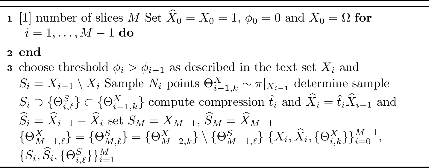
This construction adopts a frequentist view of volume estimation. A Bayesian alternative would model the compression factors \(t_i\) as Beta-distributed variables, based on the binomial sample. This would yield a hybrid strategy using Bayesian volume estimates while keeping Monte Carlo integration within each slice. In principle, a full Bayesian version is also possible if we can make prior assumptions on the target function within each slice.

3.2 Slice Monte Carlo Integration↩︎

The slicing algorithm outlined above provides a partition \(\mathscr{S}=(\mathscr{S}_1, \dots, \mathscr{S}_M)\) of the parameter space, along with prior mass estimates and prior samples, of size \(\hat{n}_i^\mathscr{S}\) for all slices \(i=1,\dots,M\). Although the function \(\phi\) is used to generate the partition, the resulting partition can be used to perform stratified Monte Carlo integration on a different \(\pi\)-integrable function \(L:\Omega\to\mathbb{R}\). Using the partition, we can rewrite the integral \[\begin{align} \label{eq:q:mean} \mathcal{Z} &= \int L(\theta)\, \mathrm{d}\pi(\theta) = \sum_{i=1}^M S_i \int L(\theta) \,\mathrm{d}\pi\vert_{\mathscr{S}_i}(\theta) = \sum_{i=1}^M S_i\, \mathbb{E}_{\pi}[L(\Theta)\vert \Theta\!\in\!\mathscr{S}_i]\,, \end{align}\tag{15}\] with the conditional mean defined as \[\mathcal{Z}_{\mathscr{S}_i} = \mathbb{E}_{\pi}[L(\Theta)\vert \Theta\!\in\!\mathscr{S}_i] = \int L(\theta) \,\mathrm{d}\pi\vert_{\mathscr{S}_i}(\theta)\]

We can use the samples within each slice generated by the slicing algorithm to estimate the integral over each slice via Monte Carlo integration. This motivates the following estimator, using slice volume estimates \(\widehat{S}_i\) and prior samples \(\{\Theta^{\mathscr{S}}_{i,k}\}\) \[\label{eq:aux1} \widehat{\mathcal{Z}} := \sum_{i=1}^M \widehat{S}_i \widehat{\mathcal{Z}}_{\mathscr{S}_i}\quad\text{with}\quad \widehat{\mathcal{Z}}_{\mathscr{S}_i} := \frac{1}{n_i}\sum_{k=1}^{n_i} L(\Theta^{\mathscr{S}}_{i,k})\,,\tag{16}\] where we only selected a subset of points available in each slice. If a fixed fraction \(\alpha_i\in(0,1]\) of the available points is evaluated in each slice, then \[\label{eq:n95i32fixed32fraction} n_i = \begin{cases} \alpha_i N_i(1-\hat{t}_i) = \alpha_i \hat{n}_i^\mathscr{S}, & i < M,\\ \alpha_M N_{M-1}\hat{t}_{M-1} = \alpha_M \hat{n}_M^\mathscr{S}, & i = M. \end{cases}\tag{17}\] In any case, we assume that at least one point falls within each slice, and that at least one point is evaluated, that is \(1 \leq n_i \leq \hat{n}_i^\mathscr{S}\).

Especially if we assume that the slicing is performed with a cheap surrogate \(\phi(\theta)\) of the target function \(L(\theta)\), the advantage of this procedure is threefold:

a) The slicing and the determination of the corresponding constrained prior masses are based on the surrogate, for which it is easy to produce large sample sizes \(N_i\), which are necessary for small uncertainties in the prior mass estimates. b) To generate uncorrelated samples from the constrained prior requires several (if not many) MC steps of some sort, where evaluations of the slicing function are necessary. This expensive step is performed on the surrogate function instead of the target function, allowing for better decorrelation of the generated samples. c) Once the slices and the corresponding prior masses are available with sufficient accuracy, we can estimate the integral over the slices with much fewer sample points, i.e. the accuracy of the slice volume and the evaluated points of the target function are decoupled. The necessary number of point evaluations per slice depends on the variance of \(L(\theta)\) within the slice, weighted by the slice’s prior mass \(S_i\). This can pose a significant advantage over standard reweighting methods, where volume uncertainty and the number of target evaluations are still coupled, as discussed in Section 2.3.

3.2.1 Unbiasedness↩︎

The estimator \(\widehat{\mathcal{Z}}\) is unbiased, i.e. \(\mathbb{E}[\widehat{\mathcal{Z}}] = \mathcal{Z}\). This follows from two observations: First, the estimator \(\hat{t}_{i}\) of the compression factor \(t_i\) is unbiased. Then \[\widehat{S}_{i} = (1-\hat{t}_i)\prod_{k=1}^{i-1} \hat{t}_k\] is unbiased for all \(i\), since \(\hat{t}_1, \ldots, \hat{t}_{M}\) are independent.

Second, the Monte Carlo estimator \(\widehat{\mathcal{Z}}_{\mathscr{S}_i}\) is conditionally unbiased for the slice expectation \(\mathbb{E}_{\pi}[L(\Theta) \vert \Theta\!\in\!\mathscr{S}_i]\).

This holds when conditioned on the sigma-field generated by the slice-membership indicators of all sampled points, \[\mathcal{F}_{\mathscr{S}} := \sigma\!\left( \mathbb{1}_{\mathscr{S}_i}(\Theta^{\mathscr{X}}_{i-1,k}) :\; i=1,\dots,M-1,\; k=1,\dots,N_i \right),\] i.e., when knowing which points fall into which sets.

Since the number \(n_i\) of selected points within slice \(\mathscr{S}_i\) and the corresponding volume estimator \(\widehat{S}_i\) are \(\mathcal{F}_{\mathscr{S}}\)-measurable, they are constant under this conditioning. So we have \[\begin{align} \begin{aligned} \mathbb{E}[\widehat{\mathcal{Z}}_{\mathscr{S}_i}\! \vert \mathcal{F}_{\mathscr{S}}] =\! \frac{1}{n_i}\sum_{k=1}^{n_i} \mathbb{E}[L(\Theta^{\mathscr{S}}_{i,k}) \vert \mathcal{F}_{\mathscr{S}}] = \mathbb{E}_{\pi}[L(\Theta) \vert\Theta\!\in\!\mathscr{S}_i] \end{aligned} \end{align}\] Together this yields \[\begin{align} \begin{aligned} \mathbb{E}[\widehat{\mathcal{Z}}] &=\sum_{i=1}^M \mathbb{E}\!\left[ \mathbb{E}\!\!\left[ \widehat{S}_i\widehat{\mathcal{Z}}_{\mathscr{S}_i} \vert \mathcal{F}_{\mathscr{S}}\right]\!\right] = \sum_{i=1}^M \mathbb{E}\!\left[ \widehat{S}_i\, \mathbb{E}\!\!\left[ \widehat{\mathcal{Z}}_{\mathscr{S}_i} \vert\mathcal{F}_{\mathscr{S}}\right]\!\right] \\ &= \sum_{i=1}^M \mathbb{E}[\widehat{S}_i]\, \mathbb{E}_{\pi}[L(\Theta) \vert\Theta\!\in\!\mathscr{S}_i] = \mathbb{E}_{\pi}[L(\Theta)] = \mathcal{Z} \end{aligned} \end{align}\]

3.2.2 Variance↩︎

In addition to unbiasedness, we are interested in the variance of the estimator \(\widehat{\mathcal{Z}}\). A detailed derivation is provided in Appendix 6; here we present the general structure and discuss its implications. The variance of \(\widehat{\mathcal{Z}}\) can be expressed as \[\begin{align} \begin{aligned} \mathrm{\mathbb{V}ar}\![\widehat{\mathcal{Z}}] = \sum_{i=1}^M \!\Bigg(\! \Delta\!\mathcal{Z}_{\mathscr{S}_i}^2 \, \mathbb{E}\left[\frac{\widehat{S}^2_{i}}{n_i}\right] + \mathcal{Z}_{\mathscr{S}_i}^2 \, \mathrm{\mathbb{V}ar}[\widehat{S}_i] + 2\mathrm{\mathbb{C}ov}[\widehat{S}_i,\!\widehat{X}_i] \, \mathcal{Z}_{\mathscr{S}_i} \, \mathcal{Z}_{\mathscr{X}_i} \! \Bigg) \end{aligned} \end{align}\] where \(n_i \leq \hat{n}_i^\mathscr{S}\) denotes the number of points selected in each slice for evaluation, with \(\hat{n}_i^\mathscr{S}\) defined in Equation 14 , and \[\begin{align} \begin{aligned} \mathcal{Z}_{\mathcal{A}} = \mathbb{E}_\pi[L (\Theta)\vert \Theta\!\in\!\mathcal{A}] \;\;\text{and}\;\; \Delta \mathcal{Z}^2_{\mathcal{A}} = \mathrm{\mathbb{V}ar}_\pi[L(\Theta) \vert \Theta\!\in\!\mathcal{A}]\,, \end{aligned} \end{align}\] denote the conditional expectation and variance over a non-empty region \(\mathcal{A}\in\{\mathscr{X}_i\}_{i=0}^{M-1}\cup\{\mathscr{S}_i\}_{i=1}^M\). For \(i=M\), the covariance contribution is interpreted as zero because \(\widehat{X}_M=0\) by convention; no conditional mean over \(\mathscr{X}_M\) is required.

This variance decomposition closely mirrors the structure of the nested sampling variance in Equation 10 that we provided in Section 2.2, but with key distinctions. In S\(\ell\)MC, discrete likelihood values are replaced by conditional expectations of the integrand within slices, and an additional term appears that accounts for intra-slice variability. While all terms depend on generally unknown properties of the integrand, they can be estimated from the available samples.

A central advantage of S\(\ell\)MC compared to standard reweighting techniques is the decoupling of volume estimation from function evaluation. The variance contribution from volume uncertainty, captured in the second and third terms, can be made arbitrarily small by increasing the number of samples \(N_i\), without incurring additional evaluations of the target function \(L\). In contrast, the first term, arising from the variance of \(L\) within each slice, can be reduced by evaluating more points per slice. If \(n_i\) is constant, it can just be pulled out of the expectation. On the other hand, if we choose to evaluate a deterministic fraction \(\alpha_i\in(0,1]\) of the points available per slice, using Equation 17 gives \[\mathbb{E}\left[\frac{\widehat{S}_i^2}{n_i}\right] = \begin{cases} \dfrac{1}{\alpha_i N_i} \dfrac{S_i}{X_{i-1}} \mathbb{E}[\widehat{X}_{i-1}^2], & i < M,\\[8pt] \dfrac{1}{\alpha_M N_{M-1}} \dfrac{S_M}{X_{M-2}} \mathbb{E}[\widehat{X}_{M-2}^2], & i = M. \end{cases}\]

This flexibility enables efficient resource allocation: volume estimation can be refined independently of the function evaluation budget. S\(\ell\)MC is therefore especially well suited for problems where the integrand exhibits low variance within each slice, as high-accuracy integration can be achieved with minimal function evaluations. To achieve this, the slicing function \(\phi\) should ideally act as a surrogate for the integrand \(L\), such that \(L\) exhibits low variability within each slice.

3.2.3 Redrawing Points for Given Thresholds↩︎

In practice, it is often beneficial to be able to redraw points for given thresholds, to increase the accuracy of the volume estimates, or to generate more points within each slice. Different slicing runs, which have the same thresholds, can be easily combined. Each slicing run \(r\) with thresholds \(\{\phi_j\}\), has samples \(\{\Theta_{j,k}^{\mathscr{X},(r)}\}\) within the level sets \(\{\mathscr{X}_j^{(r)}\}\). Assuming that the samples are independent for each run, we can simply pool them at each step of the algorithm \[\{\Theta^{\mathscr{X}}_{i,k}\} = \bigcup_{r} \{\Theta_{i,k}^{\mathscr{X},(r)}\}\quad\text{and}\quad \{\Theta^{\mathscr{S}}_{i,k}\} = \bigcup_{r} \{\Theta_{i,k}^{\mathscr{S},(r)}\}\,,\] and thereby increase the effective sample size to \(N_i = \sum_r N_i^{(r)}\), and enhance the estimate of the updated compression factors \[\hat{t}_i = \frac{\hat{n}_i^\mathscr{X}}{N_i}\,\quad\text{with}\quad \hat{n}_i^\mathscr{X} = \sum_r \hat{n}_i^{\mathscr{X},(r)}\,.\] The rest of the analysis remains the same. An adaptation of this procedure for the case of different thresholds is provided in Appendix 7.

3.2.4 Posterior Expectations and Posterior Samples↩︎

If the target function \(L\) is non-negative, we may interpret it as a likelihood function. Then the integral \(\mathcal{Z}\) is the evidence. In this case, it is also possible to compute the expectation value of a function \(g:\Omega\to\mathbb{R}\) with respect to the posterior distribution \(\mathrm{d}p(\theta)=L(\theta)\,\mathrm{d}\pi(\theta) / \mathcal{Z}\) \[\begin{align} \begin{aligned} \mathcal{G} = \int_\Omega g(\theta ) \, \frac{L(\theta)}{\mathcal{Z}} \,\mathrm{d}\pi(\theta) = \sum_{i=1}^M S_i\int g(\theta ) \, \frac{L(\theta)}{\mathcal{Z}} \,\mathrm{d}\pi\vert_{\mathscr{S}_i}(\theta) \end{aligned} \end{align}\] using S\(\ell\)MC with the previously determined sample \(\{\Theta^{\mathscr{S}}_{i,k} \}\) of the constraint prior \[\begin{align} \begin{aligned} \widehat{\mathcal{G}} = \sum_{i=1}^M \frac{\widehat{S}_i}{n_i} \sum_{k=1}^{n_i} g(\Theta^{\mathscr{S}}_{i,k} ) \, \frac{L(\Theta^{\mathscr{S}}_{i,k})}{\widehat{\mathcal{Z}}} \end{aligned} \end{align}\] Similar to NS, the slicing procedure naturally induces weighted posterior representatives \[p_{i,k} := \frac{\widehat{S}_i L(\Theta_{i,k}^{\mathscr{S}})}{n_i\, \widehat{\mathcal{Z}}}\,,\] which can be used to express the posterior expectation differently \[\begin{align} \begin{aligned} \widehat{\mathcal{G}} = \sum_{i=1}^M \sum_{k=1}^{n_i} g(\Theta^{\mathscr{S}}_{i,k} ) \, p_{i,k}\,. \end{aligned} \end{align}\] Here \(p_{i,k}\) is the probability for a parameter value \(\theta\) in a small volume of size \(\Delta V_{i}\) centered at \(\Theta^{\mathscr{S}}_{i,k}\), with \(\Delta V_{i} \approx S_i/n_i\). Note that the number of points \(n_i\) evaluated for \(g\) and \(L\) in slice \(i\) can be adjusted depending on the variability of \(g(\theta)\cdot p(\theta)\).

Beyond weighted representatives, S\(\ell\)MC also enables the generation of equally weighted samples from the posterior via approximate rejection sampling. For that purpose, we define the piecewise-constant envelope \[L^\mathscr{S} := \sum_{i=1}^M L_{\mathscr{S}_i}^{\max} \cdot \mathbb{1}_{\mathscr{S}_i}, \quad L_{\mathscr{S}_i}^{\max} := \max_{\theta \in \mathscr{S}_i} L(\theta)\,.\] As \(L_{\mathscr{S}_i}^{\max}\) is typically unknown, we have to estimate it as \(\hat{L}_{\mathscr{S}_i}^{\max} := \max \{L(\Theta_{i,k}^{\mathscr{S}})\}\) to obtain an estimated envelope \(\hat{L}^{\mathscr{S}}\).

To sample from the posterior, we first draw from the approximate (unnormalized) distribution \(\hat{L}^\mathscr{S}\) with prior distribution \(\pi\) using the estimated volumes \(\widehat{S}_i\) (see Appendix 8), and then apply rejection sampling within the selected slice \(\mathscr{S}_i\). The acceptance probability is proportional to \(L(\theta)/L_{\mathscr{S}_i}^{\max}\), from which it can be seen that the efficiency of this step depends on the within-slice variability of \(L\).

S\(\ell\)MC thus combines the variance-reduction benefits of stratification with the computational efficiency of surrogate-assisted reweighting, and provides a principled framework for adaptive slice selection and evaluation budgeting, while additionally enabling the generation of posterior samples.

4 Numerical analysis↩︎

To assess the performance of S\(\ell\)MC, we compare it to Nested Sampling (NS), reweighting with NS (RW), and Monte Carlo importance sampling (IS) on controlled benchmark problems where the surrogate quality can be varied systematically. For NS and RW, we use Skilling’s deterministic prior-mass assignment \(X_i=\exp(-i/N_{\mathrm{live}})\) to obtain point estimators \(\widehat{\mathcal{Z}}\). Details on the numerical setup for the respective methods are provided in Appendix 9. The goal is to compare how the different estimators translate surrogate mismatch into the required number of target evaluations and assess the robustness of the respective methods to surrogate-target mismatch.

4.1 Benchmark models↩︎

The benchmark models are Gaussian surrogate-target pairs. Throughout the benchmark, \(\Omega=B_1(0)\subset\mathbb{R}^d\) is the unit ball and \(\pi\) is the flat prior on \(\Omega\). The Gaussian parameters are chosen such that both \(\phi\) and \(L\) are well contained in \(\Omega\), so boundary effects are negligible and the evidence \(\mathcal{Z}=\mathbb{E}_\pi[L]\) defined in Equation 1 is given by the corresponding full-space Gaussian integral, which can be computed in closed form. Let \[\varphi_d(\theta;\mu,\Sigma) := \exp\!\left[-\frac{1}{2}(\theta-\mu)^\top\Sigma^{-1}(\theta-\mu)\right]\] denote an unnormalized Gaussian density on \(\mathbb{R}^d\). For simplicity we choose an isotropic Gaussian as surrogate \[\phi(\theta)=\varphi_d(\theta;\mu_\phi,\sigma_\phi^2 I_d)\,,\] chosen with mean \(\mu_\phi=0\) and variance \(\sigma_\phi^2=2.5\times10^{-5}\) (standard deviation \(\sigma_\phi=0.005\)).

We consider two target families – shift and anisotropy. The shift benchmark varies the relative mean displacement while keeping the variances isotropic with \(\sigma_L^2=\sigma_\phi^2\), \[L_{\mathrm{shift}}(\theta;b) =\varphi_d(\theta;\mu_L,\sigma_L^2 I_d)\,, \qquad b=\frac{\|\mu_L-\mu_\phi\|}{\sigma_L}\,.\] The anisotropy benchmark fixes the means \(\mu_L=\mu_\phi\) and varies \[\begin{align} \begin{aligned} L_{\mathrm{aniso}}(\theta;a) &=\varphi_d(\theta;\mu_L,\Sigma_L(a))\,,\\ \Sigma_L(a) &=\sigma_\phi^2\,\,\mathrm{diag}(\underbrace{a^2,\ldots,a^2}_{\lfloor d/2\rfloor}, \underbrace{a^{-2},\ldots,a^{-2}}_{\lceil d/2\rceil})\,, \quad a\ge 1\,. \end{aligned} \end{align}\] Thus, one half of the coordinate directions is stretched and the other half is compressed. Note that an isotropic mismatch would only influence the performance of IS, while the other methods are invariant to isotropic scaling of the target.

Thus the shift family probes mean mismatch, while the anisotropy family probes covariance mismatch. For the even dimensions used below, the product of all target widths in the anisotropy benchmark is independent of \(a\). For each mismatch setting, the exact value \(\mathcal{Z}\) is used to report relative errors \(\delta := |\widehat{\mathcal{Z}} \!-\! \mathcal{Z}| / \mathcal{Z}\).

4.2 Benchmarking procedure↩︎

We compare the above methods by evaluating their relative error as a function of the target-function evaluation cost \[Q:=\#\{\text{required evaluations of }L\}\,.\] Evaluations of \(\phi\) are treated as negligible and are not counted in \(Q\). For a fixed cost \(Q\), the relative error \(\delta(Q)\) is random because each method is stochastic. Writing \(\mathbb{P}[\,\cdot\,]\) for the probability distribution at fixed \(Q\) for the different methods, we define the minimal required cost for a tolerance \(\epsilon\) and success probability \(p\) as \[Q^\star(\epsilon,p)=\min\left\{Q:\;\mathbb{P}\!\left[\delta(Q)\le\epsilon\right]\ge p\right\}\,,\] which is the minimal number of point evaluations of the target function required to achieve a relative error of at most \(\epsilon\) with probability at least \(p\). For S\(\ell\)MC, RW, and NS, repeated runs at different budgets produce empirical pairs \((Q_j,\delta_j)\), which form an error–cost scatter plot as illustrated in Figure 2. We estimate \(Q^\star\) from these empirical pairs by a window-based convergence criterion and quantify uncertainty by bootstrap resampling. The method-specific numerical setup, cost mappings, and estimation procedure are described in Appendix 9. For IS, \(Q^\star\) is obtained analytically using the central limit theorem; see Appendix 10.

4.3 Results↩︎

We report benchmark results for \(d=2\), \(d=8\), and \(d=30\). For clarity, the \(d=2\) panels use \(\epsilon=0.1\), while the \(d=8\) and \(d=30\) panels use \(\epsilon=0.2\). All panels in Figure 3 show the required cost \(Q^\star(\epsilon, p=0.9)\), with bootstrap 16th/84th percentile bands for S\(\ell\)MC, RW, and NS (see Appendix 9), and analytical CLT values for IS (see Appendix 10). For IS we additionally show the effect of scaling the surrogate proposal variance by using \[\phi_\eta(\theta) =\varphi_d(\theta;\mu_\phi,\eta\sigma_\phi^2 I_d)\,, \qquad \eta\in\{0.7,1.0,1.3\}\,.\] The other methods are invariant to isotropic scaling of the surrogate, so only one curve is shown for each of S\(\ell\)MC, RW, and NS.

NS forms a constant baseline in these plots because it does not depend on the surrogate. Its cost is therefore independent of the surrogate-target mismatch by construction. The larger absolute level of NS compared with RW mainly reflects the cost model in Appendix 9.1: RW evaluates \(L\) on the stored surrogate-NS representatives, whereas direct NS pays the constrained-replacement overhead \(c_{\mathrm{NS}}\) during target-based sampling.

In the anisotropy benchmark, the top-row panels of Figure 3 show \(Q^\star\) as a function of the anisotropy parameter \(a\). Across all dimensions, IS has the lowest cost when \(a\) is close to one, as expected from its favorable behavior when the proposal is nearly identical to the target. This advantage is fragile: as soon as the surrogate is too narrow in one target direction, the importance-weight variance diverges. For the unscaled proposal, the finite-variance condition derived in Appendix 10 translates to \(a<\sqrt{2}\) for the stretched directions; with proposal variance scale \(\eta\), this boundary becomes \(a<\sqrt{2\eta}\). Thus the IS curves terminate at predictable finite-variance boundaries, and the deterioration before those boundaries is particularly pronounced.

S\(\ell\)MC and RW are more robust because they do not rely on a single global importance density with finite weight variance. Instead, both methods use the surrogate to partition the parameter space and distribute samples across the induced level sets, so their cost grows more gracefully as the surrogate-target mismatch increases. Both methods become more expensive as \(a\) increases, since the target varies more strongly inside the surrogate-induced slices, but S\(\ell\)MC remains consistently below RW over the tested range. This is the practical effect of decoupling slice-volume estimation from target evaluation: S\(\ell\)MC can spend many cheap surrogate samples on the partition and volume estimation, while only the selected integration points require expensive evaluations of \(L\). As the mismatch and thus the within-slice variance increase S\(\ell\)MC gets closer to RW, as many points within each slice are needed to obtain a small relative error. This behavior is consistent across all investigated dimensions. However, for increasing dimension the mismatch leads to higher absolute \(Q^\star\) values and more sensitive behavior with respect to the mismatch.

In the shift benchmark, the bottom-row panels of Figure 3 show \(Q^\star\) as a function of the shift parameter \(b\). Here the surrogate and target have the same shape, but their centers are displaced. IS again starts with the lowest cost near perfect agreement; for the unscaled proposal its normalized variance grows like \(\exp(b^2)\) in the isotropic shift case (Appendix 10), and the variance-scaled proposals retain the same exponential sensitivity. This is less abrupt than the anisotropy benchmark because there is no finite-variance boundary; nevertheless, the cost eventually becomes enormous as the high-mass regions of surrogate and target separate.

S\(\ell\)MC and RW are more stable under this mismatch because their surrogate-based partitions still place samples across the relevant level sets. Their costs increase with \(b\), but the growth is much slower than for IS over the range shown, and again S\(\ell\)MC remains below RW. This is consistent with the same decoupling principle: the surrogate partition can still be estimated cheaply, while target evaluations are allocated only to estimate the contributions within the resulting slices.

The two benchmark families highlight complementary failure modes. IS is optimal only when the surrogate is very accurate: it is extremely sensitive to shape mismatch, where a single overly narrow surrogate direction can make the variance infinite, and it deteriorates exponentially under pure position mismatch. RW and S\(\ell\)MC are more robust because they use the surrogate to partition the parameter space rather than using a single global importance density.

S\(\ell\)MC is typically more efficient than RW because the expensive target evaluations are decoupled from the surrogate-based volume estimation, but this advantage naturally shrinks when large mismatch forces many target evaluations within each slice. This also explains why the two curves approach each other at larger mismatch. When the target varies strongly within the surrogate-induced slices, S\(\ell\)MC must evaluate many target points per slice, so within-slice target variance dominates and slice-volume uncertainty becomes less relevant. In the same regime, the volume uncertainty in RW becomes small and the remaining uncertainty stems from the target variance along the surrogate level sets. So S\(\ell\)MC and RW have the same dominant source of uncertainty. Additionally, the effective point weights of RW and S\(\ell\)MC become similar, when RW and S\(\ell\)MC use a comparable number of points per volume. For small mismatch, in contrast, S\(\ell\)MC can achieve low error with few target evaluations per slice due to the decoupling of volume uncertainty and target evaluations, while RW still pays for the coupled volume-estimation and target-evaluation mechanism.

NS, finally, remains the surrogate-independent reference method: its cost is flat across mismatch parameters and higher than RW in the present comparison because direct constrained sampling carries the additional target-evaluation overhead.

Together, the results show that S\(\ell\)MC turns surrogate quality into reduced target-evaluation cost while retaining considerably more robustness to mismatch than direct importance sampling.

5 Conclusion and Outlook↩︎

We have introduced Slice Monte Carlo integration (S\(\ell\)MC) as a surrogate-informed integration method that uses a Nested Sampling-like construction to partition the parameter space into slices adapted to the surrogate level sets. The partition and the slice volumes are estimated using the cheap surrogate, while the expensive target function is evaluated only for the Monte Carlo estimates within the slices.

The central advantage is the decoupling of slice-volume estimation from target evaluation. Standard reweighting with Nested Sampling uses the surrogate to avoid expensive constrained sampling, but target evaluations remain tied to the quadrature resolution. S\(\ell\)MC separates these two tasks: many surrogate samples can refine the slice volumes, while the number of target evaluations can be chosen independently according to the integration budget. This additional degree of freedom explains the improved performance over reweighting observed in the benchmark problems.

Compared with classical importance sampling, S\(\ell\)MC is substantially more robust to surrogate-target mismatch. Importance sampling is most efficient when the surrogate proposal is already very close to the target, but it deteriorates rapidly when surrogate-target mismatch occurs. S\(\ell\)MC instead uses the surrogate only to define a partition of the parameter space and estimates the target contribution within each slice directly, avoiding the severe failure modes of importance sampling. The price is that, in the ideal case of nearly perfect surrogate-target agreement, direct importance sampling can require fewer target evaluations. In realistic applications, however, surrogate information is rarely perfect, and robustness to mismatch is often more valuable than optimal performance in this limiting case.

The present numerical study used a deliberately simple and uniform protocol for the number of target evaluations per slice setting \(n_i=n\) for all slices \(i=1,\ldots,M\). A natural extension is an adaptive allocation strategy in which the number of evaluated points is chosen from estimates of the target variance within each slice, as in classical stratified Monte Carlo methods [15]. This could be combined with control-variate ideas from multifidelity and multilevel Monte Carlo methods [27]–[29], for example by estimating slice-wise surrogate-target correlations. More speculatively, if several surrogate models of increasing fidelity are available, one could transfer or refine the slice partition across fidelity levels, to obtain a multilevel version of S\(\ell\)MC.

S\(\ell\)MC is particularly attractive because the hard constrained-sampling task is performed on the cheap surrogate, while the resulting slices are then used for a stratified integration of the expensive target. This makes the method relevant for applications where low-fidelity physical models are readily available [7], [8], where simplified energy landscapes can guide expensive partition-function calculations [10], [12], or where machine-learned surrogate models approximate costly high-fidelity evaluations [20]–[22], [24]. Overall, S\(\ell\)MC provides a robust and flexible framework for surrogate-informed Bayesian evidence integration when the surrogate is useful but not perfectly reliable.

References↩︎