From spectral structure to sensing limits in quantum thermometry
June 24, 2026
Abstract
The precision of a quantum thermometer is fundamentally constrained by the spectral structure of the probe itself, and a systematic mapping between the configurations of energy levels and thermometric performance provides relevant information to design optimized devices. In this work, we establish such a mapping by analyzing a broad class of quantum systems, ranging from finite spin ensembles and degenerate atoms to confining potentials, quantum walks, and continuous-spectrum models. We derive exact scaling laws for the quantum Fisher information, revealing two distinct high-temperature universality classes: finite-spectrum probes exhibit a \(T^{-4}\) decay, while unbounded or continuous spectra yield a slower \(T^{-2}\) decay. At low temperatures, we show that sensitivity, though universally exponentially suppressed, can be enhanced arbitrarily by engineering degenerate excited states or a quantum walk on a fully connected topology. By contrast, specific quantum walk topologies provide a distinct enhancement mechanism based on gap engineering, whereby an optimal network size yields an optimized \(T^{-2}\) low-temperature scaling. Furthermore, power-law spectra enable tunable scaling of thermometric performance with system size, offering a design principle for optimal probes in specific temperature windows. Our results contribute to transform spectral information into a resource for quantum thermometry, providing both fundamental bounds and practical guidelines to tailored temperature sensing.
1 Introduction↩︎
Quantum thermometry has a central role in estimation theory, not only because temperature is a fundamental parameter in virtually every physical setting, but also because thermal effects pose a persistent challenge to the control and reliability of quantum devices. Unknown temperature fluctuations can induce errors in quantum computing protocols [1]–[3], degrade the efficiency of quantum engines and refrigerators [4]–[6], and limit the reproducibility of experimental results [7], [8]. Most experiments operate at finite temperature, where the quantum system of interest is weakly coupled to an external reservoir and relaxes to a thermal state. In this general regime, estimating the environmental temperature is not just a calibration step but rather is a central part in the characterization of any equilibrium quantum system.
The development of optimized quantum thermometers is therefore crucial [9]–[21]. Quantum estimation theory provides the fundamental tools to saturate the ultimate precision bounds on temperature measurements [22], [23], and recent years have seen several proposals for experimental realizations [24]–[37]. For equilibrium sensing, which is the focus of this work, it is well known that measuring the energy of the probe saturates the quantum limit [38]–[41], regardless of temperature. However, this optimality of energy measurements does not imply universal performance across different probes. Depending on their spectral structure or critical behavior, different quantum systems can exhibit markedly different sensitivities to thermal fluctuations [42]–[45]. This immediately raises two questions: what spectral features characterize an optimal probe for equilibrium quantum thermometry? And how does this optimality depend on the underlying energy spectrum [46], [47]?
Answering these questions requires a systematic analysis of how temperature information is encoded in the equilibrium states of different classes of quantum systems. The distribution of energy levels, the presence and structure of degeneracies, the scaling of spectral gaps, and the distinction between bounded and unbounded spectra all jointly determine the low- and high-temperature sensitivity of a quantum thermometer. From this point of view, the energy spectrum itself becomes a thermodynamic resource [48] since it dictates not only the ultimate achievable precision but also the accessible temperature range and how performance scales with system size.
In this work, we develop a systematic spectral analysis of equilibrium quantum thermometry. Considering a broad class of realistic quantum systems, ranging from finite-dimensional spins and degenerate atoms to confining potentials, quantum walks, and continuous-spectrum models, we identify spectral properties as the resource governing thermometric performance. In particular, we analyze how level spacing, degeneracy structure, spectral growth, and the interplay between discrete and continuous spectral components affect the quantum Fisher information for temperature estimation. Special emphasis is placed on the low- and high-temperature regimes, where universal scaling laws emerge and allow a classification of distinct thermometric behaviors according to spectral structure. Our approach reveals which classes of spectra provide optimal probes in different temperature windows and clarifies how finite, unbounded, and mixed spectra lead to qualitatively different precision limits. Beyond comparing specific models, our results aim to establish a general framework that links the spectral structure to fundamental bounds and optimality in equilibrium quantum thermometry.
The paper is organized as follows. In Section.2, we briefly review the description of thermal quantum states, with a focus on general limits of quantum Gibbs states and on the coupling between a temperature probe and its environment. In Section 3, we examine the main theoretical tools of quantum thermometry introducing the concept of classical and quantum Fisher information, which intrinsically define the precision achievable in a temperature estimation protocol, highlighting its relation with the energy spectrum of the thermometer. In Section 4, we compare different microscopic systems as resources for temperature estimation, analyzing how spectral properties influence the scaling of precision in temperature estimation. In Section 5, we summarize the results obtained for all the methods highlighting the general properties of each model. Section 6 closes the paper with some concluding remarks. Additional details on the derivation of the general form of the QFI, as well as its high- and low-temperature limits, for specific models, can be found in the Appendix 7.
2 Thermal States↩︎
Consider an \(N\)-dimensional quantum system with Hamiltonian \[\label{eq:hamiltonian} H = \sum_{n=0}^{N-1} E_{n} \ket{\phi_{n}}\bra{\phi_{n}}.\tag{1}\] When such a system is in thermal equilibrium with an environment at temperature \(T\), its state is time-independent and given by the Gibbs state \[\label{eq:thermal95rho} {\rho}_{th} = \frac{1}{\mathcal{Z}} \sum_{n=0}^{N-1} e^{-\beta E_{n}} \ket{\phi_{n}}\bra{\phi_{n}},\tag{2}\] where \(\beta = (k_B T)^{-1}\) and \(\require{physics} \mathcal{Z} = \Tr[e^{-\beta H}]\) is the partition function. Throughout this work, we use natural units and set \(\hbar=k_B=1\).
The Gibbs state exhibits universal behavior in the extreme temperature limits, independent of the detailed spectral structure of the system. As \(T \to 0\), the state approaches the ground state: \[\label{eq:low32temperature} \lim_{T\rightarrow0} \rho_{th} = \ket{\phi_{0}} \bra{\phi_{0}}.\tag{3}\] Conversely, as \(T \to \infty\), it tends to the maximally mixed state: \[\label{eq:high32temperature} \lim_{T\rightarrow \infty } \rho_{th} = \frac{1}{N} \sum_{n=0}^{N-1} \ket{\phi_{n}} \bra{\phi_{n}}.\tag{4}\] Between these limits, the occupation of energy levels depends on both \(T\) and the system’s spectral properties.
In principle, the precise determination of an environment’s temperature requires complete knowledge of the environment Hamiltonian \(H^{e}\), the thermometer Hamiltonian \(H^{t}\), and their interaction \(V^{e-t}\). The global system is described by \[\label{eq:environment324332thermometer32Hamiltonian} H^{g} = H^{e} \otimes \mathbb{I}^{t} + \mathbb{I}^{e} \otimes H^{t} + \lambda V^{e-t},\tag{5}\] where \(\lambda\) quantifies the coupling strength. The equilibrium state of the joint system is then the Gibbs state diagonal in the eigenbasis of \(H^{g}\): \[\require{physics} \label{eq:total32gibbs} \rho^{g}_{th} = \frac{1}{\Tr[e^{-\beta H^{g}}]} \sum_{n=0} e^{-\beta E^{g}_{n}} \ket{\phi^{g}_{n}}\bra{\phi^{g}_{n}},\tag{6}\] with the superscript \(g\) denoting eigenvalues and eigenvectors of \(H^{g}\).
However, in the weak-coupling regime (\(\lambda\) sufficiently small for a given \(\beta\)), the reduced state of the thermometer can be approximated by its local Gibbs state. Tracing out the environment yields [49] \[\require{physics} \label{eq:approximation32thermal32state} \Tr_{e}\left(\rho^{g}_{th}\right) \simeq \rho^{t}_{th} + \mathcal{O}(\lambda),\tag{7}\] where \[\label{eq:thermal32state32thermometer} \rho^{t}_{th}= \frac{1}{\mathcal{Z}} \sum_{n=0} e^{-\beta E^{t}_{n}} \ket{\phi^{t}_{n}}\bra{\phi^{t}_{n}}.\tag{8}\] Thus, under weak coupling, the temperature \(T\) of the environment can be estimated using only the spectral properties of the quantum thermometer itself.
The precision of such temperature estimation depends on the energy level structure of the thermometer, and different thermometer models may perform optimally in different temperature regimes. Motivated by this, we analyze several physical models with potential thermometric applications, aiming to derive general results valid in the weak-coupling regime. Specifically, we consider quantum systems that probe the environment’s temperature under the approximation in Eq. 7 . For simplicity, we henceforth omit the superscript \(t\) and denote the thermometer’s Hamiltonian and Gibbs state as \(H\) and \(\rho_{th}\), respectively.
3 Fisher and quantum Fisher information↩︎
Temperature is usually estimated rather than measured, i.e., it is inferred by measuring some observables, whose value is temperature-dependent. This is even more true in quantum mechanics, where temperature is not an observable in strict sense. Given a preparation of a quantum system, the measurement of an observable \(Y\), and an estimator \(\hat{T}\) of temperature, the precision of the estimation strategy is bounded by the Cramèr-Rao theorem as \[\label{eq:CRB} \text{Var} \, \hat{T} \geq \frac{1}{M F_Y(T)} ,\tag{9}\] where \(M\) is number of measurements performed on the system, and \[\label{eq:fisher95information} F_{Y}(T) = \sum_{y} \dfrac{\left| \partial_{T} p \left( y \vert T \right) \right|^{2}}{p\left( y \vert T \right)},\tag{10}\] is the Fisher information. The probability density \(p\left( y \vert T \right)\) describes the distribution of the outcomes of \(Y\) given the value of temperature, and is obtained by the Born rule. The supremum of the FI, i.e. the maximization over all possible quantum measurements, is termed quantum Fisher information (QFI) and may be explicitly calculated as \[\label{eq:general95qfi} \mathcal{F}(\lambda) = Tr[\rho_{\lambda}\mathcal{L}^{2}_{\lambda}],\tag{11}\] where \(\mathcal{L}\) is the so called symmetric logarithmic derivative, defined as \[\label{eq:sld} \partial_{\lambda} \rho_{\lambda} = \frac{ \mathcal{L}_{\lambda}\rho_{\lambda} + \rho_{\lambda} \mathcal{L}_{\lambda} }{2}.\tag{12}\] For the estimation of the temperature, the optimal measurement corresponds to the energy of the system, i.e., \(F_{E}(T)=\mathcal{F}(T)\). For a state at thermal equilibrium, we have \[\label{eq:40q41fi} F_{E}(T)=\mathcal{F}(T)= \frac{\langle {(\Delta H)^{2}} \rangle}{T^{4}}.\tag{13}\] where \(\langle {(\Delta H)^{2}} \rangle\) denotes the fluctuations of the system’s Hamiltonian on the equilibrium state. In the following, we will investigate the behavior of this quantity for different systems. On the other hand, for a discrete non degenerate spectrum, we have a general expression valid in the low temperature limit, i.e. a temperature range for which the only occupied energy level are the ground state \(\ket{\phi_{0}}\) and the first excited state \(\ket{\phi_{1}}\) (i.e. \(e^{-\beta E_{2}} \simeq 0\)). In this regime, the temperature QFI may be written \[\begin{align} \label{eq:limit32qfi32small32T} {\cal F}(T) \stackrel{T \ll E_{2}}{\simeq} \frac{\left( E_{1} - E_{0} \right)^2}{4 T^4 \cosh^2\left[ (E_{1} - E_{0})/2T\right]}\,. \end{align}\tag{14}\] In the high temperature limit, and still considering a system with a finite spectrum (i.e. \(e^{-\beta E_{N-1}} \simeq 1\)), we may write \[\begin{align} \label{eq:limit32qfi32infinite32T} {\cal F}(T) \stackrel{T \gg E_{N-1}}{\simeq} & \frac{\left[ \frac{1}{N} \sum_{n} E_{n}^{2} - \frac{1}{N^2} \left( \sum_{n} E_{n} \right)^2 \right]}{T^{4}} \,. \end{align}\tag{15}\] Considering continuous or degenerate spectra, the behavior of the QFI and its low- and high-temperature limits may vary considerably. Indeed, a systematic study over the spectrum properties of quantum probes is then fundamental in order to design precise quantum thermometers.
4 Results↩︎
The results of Sec.3 indicates that the spectral distribution of energy levels in a quantum system determines how precisely the environmental temperature can be estimated, with different quantum systems yielding different precision. As an example, confined and free quantum particles exhibits different spectra ranging from a discrete to a continuous one, but temperature information is encoded in the thermal occupation of energy levels and determined by the density of states. This means that independently of the physical realization, the thermometric performances are mainly governed by the spectral structure of the quantum system itself.
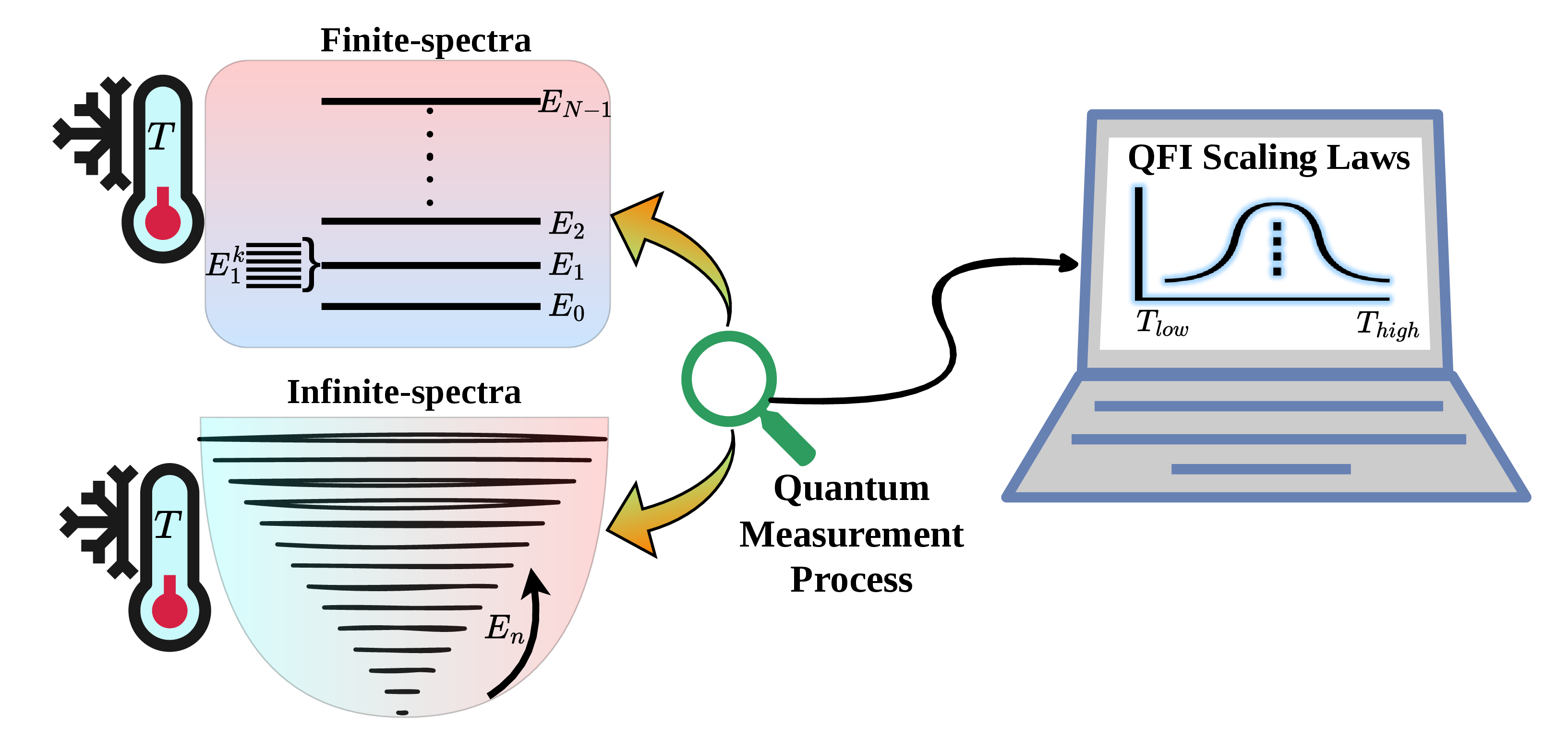
Indeed, in the following Sections we will analyze various spectra associated to paradigmatic physical systems, and we investigate how the energy level spacing affects the (Q)FI and its scaling in various temperature regimes.
4.1 Quantum thermometry using probes with finite spectrum↩︎
Let us first consider paradigmatic quantum systems having a finite spectrum.
4.1.1 Spin Systems↩︎
We begin this analysis with \(N\) dimensional spin systems. Specifically, for a spin-\(s\) particle in a uniform magnetic field \(B\) along the \(z\)-axis, the Hamiltonian can be written as \[\label{key} H^{s} = -\omega S_z, \quad \omega = \gamma B > 0,\tag{16}\] and the associated energy spectrum is \[E^{s}_m = -\omega m, \quad m = -s, -s+1, \dots, s \, ,\] i.e. \(N = 2s+1\) equally spaced levels with spacing \(\Delta = \omega\). Each energy level corresponds to a Zeeman sub-level of the spin projection along \(B\), the spectrum is symmetric and evenly spaced. The energy variance \(\mathrm{Var}(H^{s})\) may be calculated analytically and the QFI for the temperature is given by \[\begin{align} \mathcal{F}^{s} (T)&=& \frac{\omega^2}{4 T^4} \left[ \mathrm{csch}^2\left( \frac{\omega}{2 T} \right) - N^2 \mathrm{csch}^2\left( \frac{N\omega}{2 T} \right) \right].\nonumber\\ \end{align}\] This QFI expression, obtained for spin systems, is valid for every physical model with evenly spaced energy levels, the difference will be in terms of energy shift \(\Delta\). The expression highlights the role of spectral boundedness. In turn, the first term has the same functional form as a single quantum harmonic oscillator QFI, see 32 , reflecting the equally spaced nature of energy levels. The second term, which depends explicitly on \(N\), originates from the finite-dimensional nature of the spectrum. Finite spin systems can indeed be interpreted as truncated harmonic oscillators, continuously approaching the harmonic oscillator behavior in the limit \(N \to \infty\).
Let us now address the asymptotic behavior of the QFI at low- and high-temperature (see App. 7.1). At low temperature the QFI behaves as \[\label{eq:low32T32spin} \mathcal{F}^{s}(T) \simeq \frac{\omega^2}{T^4} e^{-\omega/T},\tag{17}\] which depends only on the lowest energy gap (see Eq.@eq:eq:limit32qfi32small32T ). For \(T \to \infty\) we have \[\mathcal{F}^{s}(T) \simeq \frac{\omega^2}{12 T^4} \left(N^2 - 1\right).\] At low temperature the QFI is exponentially suppressed, since only the first excited level contributes, whereas at high temperature the QFI decays as \(T^{-4}\), with a prefactor that scales as \(N^2\).
4.1.2 \(N\)-level atom with ground state + \((N-1)\) degenerate excited states↩︎
Here, we consider an atom with a non-degenerate ground state and an \((N -1)\)-fold degenerate excited level Hamiltonian, \[H^{N} = E_0 \ket{\phi_{0}}\bra{\phi_{0}} + E_{1} \sum_{n=1}^{N-1} \ket{\phi_{n}}\bra{\phi_{n}} \, .\] In this way we can address how degeneracy of energy levels influence temperature estimation precision in discrete spectra. It was previously demonstrated that this model is the optimal quantum thermometry probe under specific conditions [24]. Without loss of generality the energy spectrum can be written as \[\label{eq:spectrum95atom95degenerate} E^{N}_0 = 0, \quad E^{N}_1 = E^{N}_2 = \cdots = E^{N}_{N-1} = \epsilon.\tag{18}\] The energy variance of such model is \[\mathrm{Var}(H^N) = \frac{(N-1)\epsilon^2 e^{-\beta\epsilon}}{[1 + (N-1)e^{-\beta\epsilon}]^2},\] and consequently the QFI for temperature, \[\label{eq:fisher95atom95degenerate} \mathcal{F}^{N}(T) = \frac{1}{T^4} \cdot \frac{(N-1)\epsilon^2 e^{-\beta\epsilon}}{[1 + (N-1)e^{-\beta\epsilon}]^2}.\tag{19}\]
In the low temperature limit, \(T \to 0\) (\(\beta \to \infty\)), the Boltzmann factor satisfies \(e^{-\beta\epsilon} \ll 1\), so that only the ground state and the first excited manifold contribute appreciably. Keeping the leading exponential contribution, the QFI reduces to \[\label{eq:low95T95QFI95atom95degenerate} \mathcal{F}^{N}(T) \simeq \frac{(N-1)\epsilon^2}{T^4} e^{-\epsilon/T}.\tag{20}\] Thus, at low temperature the thermometric sensitivity is exponentially suppressed by the spectral gap \(\epsilon\), while the prefactor is enhanced by the excited-state degeneracy \((N-1)\) (compare with Eq.@eq:eq:low32T32spin to explicitly see the effect of degeneracy).
For high-temperature \(T \to \infty\) (\(\beta \to 0\)), the Gibbs state approaches a uniform distribution over the \(N\) levels. Expanding the Boltzmann factor to leading order, \(e^{-\beta\epsilon}\simeq 1 + \mathcal{O}(\beta)\), the partition function becomes \(Z \simeq N\), and the QFI simplifies to \[\label{eq:high95T95QFI95atom95degenerate} \mathcal{F}^{N}(T) \simeq \frac{(N-1)\epsilon^2}{N^2 T^4}.\tag{21}\] At high temperature, the QFI decays as \(T^{-4}\), and the \(N\)-dependent prefactor shows that strong degeneracy does not lead to a quadratic enhancement at high temperature. Then, overall, at low temperature, the QFI scales with \(N\), while at high-T, decreases with \(N\).
4.1.3 Quantum walks↩︎
When a quantum system can be modeled as a collection of n qubits (nodes) that form a network connected by a specific topology, it may be described using the quantum walk (QW) formalism. The system is described by an excitation-preserving Hamiltonian in the form \[\begin{align} \label{eq:total95Hamiltonian95QWs} {H}^{QW} = \sum_{i=0}^{N-1} \omega_{i} \left( \sigma_{i}^{+}\sigma_{i}^{-} \right) + \sum_{i,j = 0}^{N-1} g_{i,j}\left( \sigma_{i}^{+}\sigma_{j}^{-} + \sigma_{j}^{+}\sigma_{i}^{-} \right), \end{align}\tag{22}\] where \(\sigma_{i}^{\pm}\) represent the ladder operators of the qubit \(i\), \(\omega\) represent the on-site energy and \(g_{ij}\) the hopping strength. In single excitation regime and under the condition of isotropy \(g_{ij}=-\mathcal{J}\) and \(\omega_{i}=\omega \cdot deg(i)\), i.e. proportional to the degree (number of connections) of the node \(i\), the QW Hamiltonian is reduced to \[\begin{align} \label{eq:Hamiltonian95QWs95se} \bra{i}{H}^{QW}\ket{j} = \begin{cases} 0 \; \text{if i,j are not connected} \\ \omega_{i} \cdot deg(i) \; \text{if i=j} \\ -\mathcal{J} \; \text{if i,j are connected} \end{cases}. \end{align}\tag{23}\] Different topologies are associated to different Hamiltonians and consequently to different thermometric properties. A topology in which all the qubits are connected among each others has a Hamiltonian in the form \[\label{eq:H95Complete95Network} H^{c} = N \omega \mathbb{I} - \mathcal{J}\sum_{i>j} \ket{i}\bra{j} + \ket{j}\bra{i},\tag{24}\] and was proven to be a useful resource in previous estimation applications of the model [50]. Since the spectrum of the graph is exactly the same as Eq.@eq:eq:spectrum95atom95degenerate , the thermometric results reproduce the properties of an effective two-level atom with ground state energy \(E_{0}=n\omega - (n-1)\mathcal{J}\) and \((N-1)\) and a maximally degenerate excited state \(E_{1} = n\omega - \mathcal{J}\), i.e. Eq.@eq:eq:fisher95atom95degenerate . Consequently also the high and low temperature limits are the same as Eq.@eq:eq:low95T95QFI95atom95degenerate and Eq.@eq:eq:high95T95QFI95atom95degenerate . This means that under the conditions expressed in [24] a QW model with a fully connected topology can be adopted as the optimal probe for quantum thermometry. The strength of this model relies also in the possibility to tune the values of \(\omega\) and \(\mathcal{J}\) by applying a localized electric field or by changing the distance among the different qubits [51]–[53].
Previous studies on the topology of the network have demonstrated that also the ring topology is a good candidate for thermometric applications [54]. The Hamiltonian of such topology can be expressed as \[\label{eq:H95Ring} H^{r} = 2 \omega \mathbb{I} - \mathcal{J}\sum_{i} \ket{i}\bra{i+1} + \ket{i+1}\bra{i},\tag{25}\] with the periodic boundary conditions \(\ket{n+1}=\ket{1}\). The energy levels are \[{E}^{r}_{l} = 2 \omega -2 \mathcal{J}\cos \left( \frac{2\pi(l+1)}{N} \right) \; ; \; l = 0,...,N-1 .\] Here we will focus on the study of the role of \(\mathcal{J}\) as it was proven to be a fundamental resource in other physical applications [51], [55]. Changing the value of \(\mathcal{J}\) it is possible to modify the gap between two successive energy levels and to enlarge or reduce the bandwidth of the system, i.e., the difference between the maximum and the minimum eigenvalue of the system’s Hamiltonian. The temperature QFI of such energy spectrum is \[\begin{align} \label{eq:32variance32ring32qw} &\mathcal{F}^{r}(T) = \frac{4\mathcal{J}^2}{T^4} \bigg[ \frac{\sum_{l=0}^{N-1} \cos^2\left(\frac{2\pi(l+1)}{N}\right) e^{2\beta\mathcal{J} \cos\left(\frac{2\pi(l+1)}{N}\right)}}{\sum_{l=0}^{N-1} e^{2\beta\mathcal{J} \cos\left(\frac{2\pi(l+1)}{N}\right)}} \nonumber \\ &- \left( \frac{\sum_{l=0}^{N-1} \cos\left(\frac{2\pi(l+1)}{N}\right) e^{2\beta\mathcal{J} \cos\left(\frac{2\pi(l+1)}{N}\right)}}{\sum_{l=0}^{N-1} e^{2\beta\mathcal{J} \cos\left(\frac{2\pi(l+1)}{N}\right)}} \right)^2 \bigg]\,. \end{align}\tag{26}\] The low- and high-temperature limits of Eq. 26 capture the essential thermometric behavior of the model. In the low-temperature regime \(T \to 0\), only the ground and first excited levels contribute. The energy gap scales as \(\Delta \sim 4\pi^2 \mathcal{J}/N^2\), with a two-fold degeneracy of the first excited state. The QFI therefore takes the following form \[\mathcal{F}^{r}(T) \simeq \frac{32\pi^4 \mathcal{J}^2}{N^4 T^4} \exp\!\left[-\frac{4\pi^2 \mathcal{J}}{N^2 T}\right].\] This expression shows a competition between two \(N\)-dependent mechanisms, i.e., decreasing the gap with increasing \(N\) enhances thermal accessibility, while the prefactor scales as \(N^{-4}\) and suppresses fluctuations. As a consequence, for fixed temperature \(T\) the QFI exhibits a non-monotonic dependence on \(N\) with an optimal system size determined by the balance between exponential suppression and algebraic suppression, typically scaling as \(N_{\mathrm{opt}} \sim \pi \sqrt{2\mathcal{J}/T}\).
In the opposite high-temperature regime \(T \to \infty\) at fixed \(N\), all levels become equally populated and the QFI reduces to a finite-size expression independent of spectral resolution \[\mathcal{F}^{r}(T) \simeq \frac{2\mathcal{J}^2}{T^4}.\] The interesting aspect of this model is that by varying \(N\), one may observe the transition from a discrete to a continuous spectrum. Indeed, if the thermodynamic limit \(N \to \infty\) is taken before the low and high-temperature expansions, Eq.@eq:eq:32variance32ring32qw rewrites as \[\label{eq:32variance32ring32qw32th32limit} \mathcal{F}^{r}(T) \simeq \frac{4\mathcal{J}^2}{T^4} \left[ \frac{1}{2} \left( 1 + \frac{I_2(2\beta\mathcal{J})}{I_0(2\beta\mathcal{J})} \right) - \left( \frac{I_1(2\beta\mathcal{J})}{I_0(2\beta\mathcal{J})} \right)^2 \right],\tag{27}\] where \(I_n(x)\) define the modified Bessel function of the first kind. The low and high temperature limits of the above expression are, respectively, \[\label{eq:32low32T32ring} \lim_{T \to 0} \mathcal{F}^{r}(T) \simeq \frac{1}{2T^2} \, ,\tag{28}\] and \[\label{eq:32high32T32ring} \lim_{T \to \infty} \mathcal{F}^{r}(T) \simeq \frac{2\mathcal{J}^2}{T^4} \, .\tag{29}\]
All finite spectrum probes considered in this work exhibit the same qualitative thermometric behavior. At low temperatures, in agreement with the general bounds derived in Refs. [56]–[59], the QFI is exponentially suppressed and determined by the smallest energy gap. In this context, quantum walks on fully connected networks provide a way to increase low temperature QFI through the degeneracy of the first excited state, with the exponential dependence on the gap that remains unchanged. On the other hand, for quantum walks on ring topologies, by tuning the system size, the first energy gap closes as \(1/N^2\), and the usual exponential factor becomes \(e^{-2}\) at an optimal size \(N_{opt}\) and the result is a power-law \(T^{-2}\) scaling instead of the standard exponential suppression. At high temperatures, the QFI decays algebraically and is determined by the energy variance \[\mathrm{Var}(H)\le \frac{(E_{\max}-E_{\min})^2}{4},\] the sensitivity is ultimately limited by the spectral bandwidth of the probe. Therefore, any enhancement with increasing system size can only arise from an increase in the bandwidth rather than from degeneracy alone.
4.2 Quantum thermometry using confined probes↩︎
As a second prototypical class of models, we focus on systems defined by a confining potential, such as quantum wells and harmonic oscillators. These models are well suited to describe a large variety of physical systems and quantum devices [60], [61]. Additionally, they provide examples of systems with an infinite spectrum or under some specific approximation, systems with a continuous one (see the following subsections for further details).
4.2.1 Quantum harmonic oscillator↩︎
As a first confining potential we look at the quantum harmonic oscillator (QHO), as it represents an ubiquitous model in quantum sensing and generally in physics [62]–[64]. The Hamiltonian of a harmonic oscillator \(k\) can be written in the form \[\label{eq:QHO} H^{qho}_{k} = \frac{p_k^2}{2m} + \frac{1}{2} m\omega^2 x_k^2,\tag{30}\] and describe, at least to a first approximation, any vibrational modes of a quantum system. For \(N\) independent identical oscillators of frequency \(\omega\), the hamiltonian can be written as \[H^{QHO} = \sum_{k=1}^{N} H^{qho}_{k} = \sum_{k=1}^{N} \omega \left( n_k + \frac{1}{2} \right) \ket{n_k}\bra{n_k},\] and the energy variance is additive: \[\label{eq:additive} \mathrm{Var}(H^{QHO}) = \sum_{k=1}^{N} \mathrm{Var}(H^{qho}_k) = N \omega^2 \bar{n}(\bar{n}+1).\tag{31}\] Such that the total QFI is given by \[\label{QFI95QHO} \mathcal{F}^{QHO}_{\omega}(T) = N \frac{\omega^2}{4 T^4} \, \mathrm{csch}^2\left( \frac{\omega}{2 T} \right).\tag{32}\] For a multimode system with different frequencies \(\omega_k\), we have \[\mathcal{F}^{QHO}_{\omega_k}(T)=\frac{1}{T^4}\sum_{k=1}^N \omega_k^2 \frac{e^{\beta\omega_k}}{\big(e^{\beta\omega_k}-1\big)^2}.\] If we assume a sufficiently large modes, we can apply the thermodynamic limit. For a continuous set of modes with frequencies \(\omega_k\) and density of states \(g(\omega)\), replacing the sum with an integral, the QFI reads \[\mathcal{F}^{QHO}_{\text{cont}}(T) = \frac{1}{T^4} \int_0^{\omega_c} g(\omega) \omega^2 \frac{e^{\beta \omega}}{(e^{\beta \omega}-1)^2} \, d\omega.\] For a general power-law behavior of the density of states \[g(\omega) = A \, \omega^s, \qquad 0 \le \omega \le \omega_c,\] with cutoff \(\omega_c\), and \(A\) is a normalization constant, the variance of the Hamiltonian reads \[\begin{align} \mathrm{Var}(H) &=& \int_0^{\omega_c} A \, \omega^s\, \omega^2 \frac{e^{\beta \omega}}{(e^{\beta \omega}-1)^2} \, d\omega. \end{align}\] Changing variable \(y = \beta \omega\), \(d\omega = dy/\beta\), the QFI becomes \[\mathcal{F}_{\text{cont}}(T) = A\, T^{s-1} \int_0^{\beta \omega_c} y^{s+2} \frac{e^y}{(e^y-1)^2} \, dy.\] At low temperatures (\(T \ll \omega_c\)), the QFI scales as \(\mathcal{F}_{\text{cont}}(T) \propto T^{\,s-1}\), while at high temperatures (\(T \gg \omega_c\)) it approaches the classical scaling of free particles, i.e., \(\mathcal{F}_{\text{cont}}(T) \propto 1/T^2\).
The quantum harmonic oscillator, therefore, provides a unified framework connecting discrete and continuous thermometry through the structure of its mode distribution. For a finite number of modes, additivity of independent oscillators yields a linear enhancement \(\mathcal{F} \sim N/T^2\) at high temperatures, showing the characteristic \(1/T^2\) scaling. In the continuum limit, the QFI is governed by the density of states \(g(\omega) \propto \omega^s\), at low temperatures \(T \ll \omega_c\), thermal occupation is effectively restricted to low-frequency modes, so the QFI inherits the spectral weight near \(\omega = 0\), giving \(\mathcal{F} \propto T^{s-1}\). At high temperatures \(T \gg \omega_c\), spectral structure becomes irrelevant, and the system universally recovers \(\mathcal{F} \propto 1/T^2\).
4.2.2 Quantum Rotor↩︎
After the description of the thermometric properties of a quantum harmonic oscillator, which can be adopted to model of the vibrational modes of any quantum system, we now focus on a model which can describe rotational modes [65]. Together those two models represent the basis of the quantum description of the degrees of freedom of any quantum rigid system. Because of the additive property of the energy variance (Eq.@eq:eq:additive ) we can focus on the properties of the partition function of a single quantum rotor to study the main properties of the model. The Hamiltonian of such systems can be written as \[\label{eq:QR} H^{qr} = \frac{\hat{L}^2}{2I} \, ,\tag{33}\] where \(\hat{L}\) and \(I\) are respectively the angular and inertia momentum. This Hamiltonian leads to energy levels in the form \[\label{eq:eQR} E^{qr}_{n} = \frac{1}{2I} n(n+1),\tag{34}\] each one with degeneracy \(g_n = 2n +1\). The temperature QFI of a quantum rotor is \[\begin{align} \label{eq:QFI32rotor32full} \mathcal{F}^{qr}(T) = \left( \frac{1}{2I T^2} \right)^2 &\bigg[ \frac{\sum_{n} g_n h_n^2 e^{-\beta E^{qr}_{n} } }{\sum_{n} g_n e^{-\beta E^{qr}_{n}} } - \nonumber \\ &\left( \frac{\sum_{n} g_n h_n e^{-\beta E^{qr}_{n} } }{\sum_{n} g_n e^{-\beta E^{qr}_{n}} } \right)^2 \bigg], \end{align}\tag{35}\] with \(h_n = n(n + 1)\).
For \(T \to 0\), only the lowest energy levels are thermally populated. The ground state \(n=0\) has energy \(E_0 = 0\) and degeneracy \(g_0 = 1\). The QFI in this regime thus reads \[\mathcal{F}^{qr}(T) \simeq \frac{3\Delta^2}{T^4} e^{-\Delta/T},\] with degeneracy contributing an extra prefactor \(g_1=3\). For high-temperature \(T\rightarrow\infty\) many levels contribute and the sum can be approximated by an integral. Yet, the scaling is unaffected and at high-T the QFI one has \[\mathcal{F}^{qr}(T) \simeq \frac{1}{T^2}.\] The quantum rotor has an infinite and unbounded spectrum, so the number of thermally accessible states increases with temperature. As a consequence, the energy variance grows as \(T^2\) and the QFI decays as \(T^{-2}\) (See App. 7.2 for details on the derivation of all the results related to the quantum rotor).
4.2.3 Quantum Wells↩︎
One of the easiest yet widely adopted confined model consist in considering a system with a Hamiltonian in the form \[\label{eq:QWs} H^{qw} = \frac{\hat{p}^2}{2m} + \hat{V}({x}_{k}),\tag{36}\] where \[\label{eq:VQWs} \hat{V}({x}_{k})=\begin{cases} \infty, \,\, if \,\, \abs{x_k} > d_k, \\ \; 0, \,\, if \,\,\, \abs{x_k} < d_k. \end{cases}\tag{37}\] Despite the simplicity of the model, this Hamiltonian provides a convenient description for semiconductor hetero-structures or quantum dots [61]. Following the results presented in Eq.@eq:eq:additive , we consider a \(1D\) infinite quantum well of width \(d\), whose energy spectrum is \[E^{qw}_n = \frac{n^2 \pi^2}{2m d^2}, \quad n = 1, 2, 3, \dots\] we can simplify it by writing it as \(E_n = \alpha n^2\), with \(\alpha = \frac{\pi^2}{2m d^2}\). This spectrum has a level spacing growing linearly with \(n\) i.e., \(\Delta E_n = E_{n+1} - E_n = \alpha (2n + 1)\). The QFI for the quantum Wells model reads \[\mathcal{F}^{qw}(T) =\frac{1}{T^4}\bigg[ \frac{ \vartheta_3''(0,e^{-\alpha \beta}) }{\vartheta_3(0,e^{-\alpha \beta}) - 1} - \left( \frac{ \vartheta_3'(0,e^{-\alpha \beta}) }{\vartheta_3(0,e^{-\alpha \beta}) - 1} \right)^2 \bigg],\] with \(\vartheta_3'(0,e^{-\alpha \beta})\) and \(\vartheta_3''(0,e^{-\alpha \beta})\) denoting, respectively, the first and second derivatives of the Jacobi theta function with respect to the inverse temperature \(\beta\) (see App. 7.3).
In the low-temperature limit \(T \to 0\), the QFI reads \[\mathcal{F}^{qw}(T) \simeq \frac{9\alpha^2}{T^4} \, e^{-3\alpha/T}.\] The energy gap between the ground state and the first excited state is \(E_2 - E_1 = 3\alpha\). The low-temperature scaling follows the universal form.
For the high-temperature limit \(T \to \infty\), i.e., \(\beta \to 0\), the QFI reads \[\mathcal{F}^{qw}(T) \simeq \frac{1}{2T^2}.\] Thus, the thermometric sensitivity exhibits the universal high-temperature scaling characteristic of systems with effectively unbounded spectra.
4.2.4 Power-law spectral model↩︎
After the characterization of the thermometric performances of different confined probes, a key question to address is how the QFI of such systems scales with system size and the structure of the energy spectrum. In confined thermometry, where quantum states are trapped in finite domains, the energy spectrum is inherently discrete, and its growth with the quantum number \(n\) determines the ultimate temperature sensitivity. To systematically investigate this, we consider a family of models where the energy levels follow a power-law \[E_n = C n^\alpha, \qquad n = 0,1,2,\dots, N-1,\] with \(C > 0\) setting the overall energy scale, \(\alpha > 0\) determining the growth rate of the spectrum, and \(N\) the total number of bound states (which may be finite or infinite). This spectral form naturally emerges in confined systems i.e,, \(\alpha = 1\) corresponds to evenly spaced levels such as those of a harmonic oscillator. \(\alpha = 2\) describes the quadratic dispersion of a particle in quantum wells or a strongly anharmonic confining (Morse) potential.
At sufficiently low temperatures, only the ground state and first excited state are thermally populated. Given that \(\Delta = E_1 - E_0 = C\) and assuming non-degenerate levels, the low-T QFI follows the universal form \[\mathcal{F}^{\text{low}}(T) \simeq \frac{C^2}{T^4} e^{-C/T}.\] For high-temperature , we distinct two scenarios corresponding to the case of finite and infinite spectrum. Firstly, when the temperature is much larger than the highest energy level, all \(N\) states are equally populated. The QFI is then determined by the spectral variance \[\mathrm{Var}(H) = \frac{1}{N}\sum_{n=0}^{N-1} E_n^2 - \left(\frac{1}{N}\sum_{n=0}^{N-1} E_n\right)^2,\] as provided in Eq. 15 . Redefining the sums as \[S_1(\alpha,N) = \sum_{n=0}^{N-1} n^\alpha, \qquad S_2(\alpha,N) = \sum_{n=0}^{N-1} n^{2\alpha},\] for large \(N\), we can perform the approximations \[\begin{align} S_1 \simeq \frac{N^{\alpha+1}}{\alpha+1}, \quad S_2 \simeq \frac{N^{2\alpha+1}}{2\alpha+1}, \end{align}\] leading to a QFI in the form \[\label{eq:32PL95high4432finite} \mathcal{F}^{\text{high, finite}}(T) \simeq \frac{C^2 N^{2\alpha}}{T^4} \cdot \frac{\alpha^2}{(2\alpha+1)(\alpha+1)^2}.\tag{38}\] Therefore, finite spectra exhibit the universal bounded-system scaling \(\mathcal{F}\propto T^{-4}\), while the dependence on the spectral exponent \(\alpha\) determines how thermometric sensitivity scales with the spectral span \(E_{\max}\sim N^\alpha\).
On the other hand, for an infinite number of states, the partition function at high \(T\) is \[\begin{align} Z \simeq \int_0^{\infty} e^{-C x^\alpha/T} dx = \frac{\Gamma(1/\alpha)}{\alpha} \left(\frac{T}{C}\right)^{1/\alpha}, \end{align}\] where \(\Gamma(x)\) denotes the Euler Gamma function with \(\Gamma(x)=\int_0^\infty t^{x-1}e^{-t}\,dt\). The mean energy is \[\begin{align} \langle H \rangle = \frac{1}{Z} \frac{1}{\alpha \beta} (\beta C)^{-1/\alpha} \Gamma\left(1+\frac{1}{\alpha}\right) = \frac{T}{\alpha}. \end{align}\] Similarly, for \(\langle H^2 \rangle\): \[\begin{align} \langle H^2 \rangle \simeq \frac{T^2}{\alpha} \left(1 + \frac{1}{\alpha}\right). \end{align}\] Therefore, the QFI for the infinite spectrum at high temperature is \[\label{eq:32PL95high4432infinite} \mathcal{F}^{\text{high, infinite}}(T) \sim \frac{1}{\alpha T^2}.\tag{39}\] The scaling with system size depends strongly on the exponent \(\alpha\), for \(\alpha=1\) the QFI grows quadratically (\(\mathcal{F} \sim N^2\)), for \(\alpha=2\) it grows quartically (\(\mathcal{F} \sim N^4\)), while for \(\alpha=1/2\) it grows linearly (\(\mathcal{F} \sim N\)). This shows that rapidly increasing spectra lead to a strong enhancement of thermometric sensitivity. On the other hand, for an unbounded spectrum, the QFI no longer depends on \(N\) and instead follows a universal scaling indicating a slower decay with temperature compared to finite systems, as shown in Eq.@eq:eq:32PL95high4432finite .
4.3 Quantum thermometry using systems with hybrid spectra↩︎
We now consider a class of quantum systems whose energy spectrum contains both discrete bound states and a continuous part. Such situations arise naturally in many physical systems [66], [67]. However, the canonical partition function can be written in the form \[Z(\beta) = \sum_{n} g_n e^{-\beta E_n} + \int_{E_c}^{\infty} dE\, \rho(E) e^{-\beta E},\] where \(E_n\) and \(g_n\) denote the discrete energy levels and their degeneracies, \(\rho(E)\) is the density of states of the continuum, and \(E_c\) is the threshold energy above which the spectrum becomes continuous. We now derive the asymptotic behavior of QFI in both regimes low- and high-\(T\). To proceed with the calculations we assume that the system possesses a non-degenerate ground state \(E_0\), and the first excitation gap is \(\Delta = E_1 - E_0 > 0\). Additionally, without loss of generality we consider that the continuum spectrum starts at \(E_c > E_1\), with the additional condition that the discrete spectrum is completely below the continuum threshold \(E_{c}\). The density of states near threshold behaves as \[\rho(E) \simeq C (E - E_c)^s, \quad E \gtrsim E_c.\]
The QFI for this scenario separates into the following contributions \[\mathcal{F}(T)= \mathcal{F}_{d}(T) +\mathcal{F}_{c}(T) +\mathcal{F}_{dc}(T),\] where \[\mathcal{F}_{d}=\frac{p_d\,\mathrm{Var}_d}{T^4}, \quad \mathcal{F}_{c}=\frac{p_c\,\mathrm{Var}_c}{T^4}, \quad \mathcal{F}_{dc}= \frac{p_d p_c(\mu_d-\mu_c)^2}{T^4}.\] The QFI naturally separates into discrete, continuum, and mixed contributions (see appendix 7.4 for more details). The first two terms quantify thermal fluctuations within each spectral sector, whereas the mixed-term originates from the separation of their mean energies and becomes relevant when both cases are appreciably populated.
In the low-temperature limit \(T \to 0\) (\(\beta \to \infty\)), the QFI takes the universal form \[\mathcal{F}(T) \simeq \frac{g_1 \Delta^2}{T^4} \exp\!\left(-\frac{\Delta}{T}\right).\] In the opposite limit \(T \to \infty\) (\(\beta \to 0\)), the discrete contribution becomes negligible compared to the continuum, and the QFI behaves as \[\mathcal{F}(T) \simeq \frac{s+1}{T^2}.\] The exponent \(s\) characterizes the threshold behavior of the continuum density of states. For a free particle, \(s=-1/2\) corresponds to a 1D system, \(s=0\) to a 2D system a constant density of states, and \(s=1/2\) to a 3D system.
4.4 Quantum thermometry using atomic and molecular probes↩︎
Since the miniaturization of modern technologies have led to the application of atomic or molecular system as quantum sensors [68]–[70] we also focus on the study of the thermometric performances of such physical models.
4.4.1 Hydrogen-like systems↩︎
The most used model to describe atomic systems is the hydrogen-like atom, whose spectrum arises from the Coulomb interaction and can be systematically refined through fine-structure, hyperfine-structure, and Zeeman corrections. For the hydrogen-like atom, the full Hamiltonian reads \[H = H_{\mathrm{C}} + H_{\mathrm{fs}} + H_{\mathrm{hfs}},\] where each contribution is defined as \[H_{\mathrm{C}} = \frac{\mathbf{p}^2}{2m} - \frac{Z e^2}{4\pi\epsilon_0 r}=\frac{\mathbf{p}^2}{2m} + V(r).\] This Hamiltonian yields the well-known hydrogen spectrum \[E_n^{(0)} = -\frac{m Z^2 e^4}{2(4\pi\epsilon_0)^2}\frac{1}{n^2}, \quad n=1,2,\dots\] Each energy level exhibits an \(n^2\) degeneracy (excluding the spin degree of freedom). Fine structure corrections arise from relativistic effects and spin–orbit coupling, and are described by \[H_{\mathrm{fs}} = H_{\mathrm{rel}} + H_{\mathrm{SO}} + H_{\mathrm{D}},\] with \[\begin{align} \begin{cases} H_{\mathrm{rel}} &= -\frac{\mathbf{p}^4}{8m^3c^2}, \\ H_{\mathrm{SO}} &= \frac{1}{2m^2c^2}\frac{1}{r}\frac{dV}{dr}\,\mathbf{L}\cdot\mathbf{S}, \\ H_{\mathrm{D}} &= \frac{1}{8m^2c^2}\nabla^2 V \end{cases}. \end{align}\] The resulting spectrum of Coulomb + fine structure Hamiltonian depends on the total angular momentum \(j\) and reads \[E_{n j} = mc^2 \left[ 1+\left( \frac{Z\alpha}{n-j-\frac{1}{2} + \sqrt{(j+\frac{1}{2})^2 - Z^2\alpha^2}} \right)^2 \right]^{-1/2}.\] Where \(\alpha=\frac{e^2}{4\pi\epsilon_0 c}\). In the regime \(Z\alpha \ll 1\), corresponding to weak relativistic effects. The energy can be expanded perturbatively in powers of \((Z\alpha)^2\). Thus, the fine structure expression reads \[E_{n j} \simeq E_n^{(0)} \left[ 1+\frac{(Z\alpha)^2}{n} \left( \frac{1}{j+\frac{1}{2}}-\frac{3}{4n} \right) \right].\]
The hyperfine interaction between the nuclear spin \(\mathbf{I}\) and the electronic angular momentum \(\mathbf{J}\) is described by \[H_{\mathrm{hfs}} = A\,\mathbf{I}\cdot\mathbf{J} = \frac{A}{2} \left( \mathbf{F}^2 - \mathbf{I}^2 - \mathbf{J}^2 \right),\] where \(\mathbf{F}=\mathbf{I}+\mathbf{J}\) is the total angular momentum.
The total Hamiltonian \(H_{\mathrm{C}}+H_{\mathrm{fs}}+H_{\mathrm{hfs}}\) remains diagonal in the basis \(\ket{n,j,F,m_F}\) and yields the spectrum \[E_{n j F} = E_{n j} + \frac{A}{2} \left[ F(F+1) - I(I+1) - J(J+1) \right],\] with \[F = |I-J|, \dots, I+J.\] Hydrogen-like atoms provide a natural platform for sensing in general since their energy spectra are well characterized and highly sensitive to external perturbations. Such systems offer a conceptually simple and broadly applicable framework for quantum thermometry. The energy spectrum for the total Hamiltonian reads \[E_{n j F} = E_n^{(0)} + \Delta_{\mathrm{fs}}(n,j) + \Delta_{\mathrm{hfs}}(n,j,F),\] with degeneracy \[g_{n j F} = 2F+1.\] For this model, there is no specific simplification of the formula for the quantum Fisher information of the temperature. Therefore, for convenience, we will refer to Eq.@eq:eq:40q41fi . Nonetheless in the low and high temperature limits interesting trends emerges. At sufficiently low temperatures, only the ground-state hyperfine manifold is populated. For hydrogen, with \(n=1\) and \(j=1/2\), the hyperfine splitting between \(F=0\) and \(F=1\) is \(\Delta_{\mathrm{hfs}} = A\), with degeneracies \(g_0 = 1\) and \(g_1 = 3\). The QFI for this effective two-level system reads \[\mathcal{F}_T^{\mathrm{low}}(T) \simeq \frac{3A^2}{T^4} e^{-A/T}.\] At high temperature the Boltzmann factors can be expanded as \[e^{-\beta E_n} \simeq 1 - \beta E_n + \mathcal{O}(\beta^2).\] In this regime, fine and hyperfine splittings become negligible, and the spectrum can be approximated by the hydrogenic energies \[E_n = -\frac{E_0}{n^2}, \quad g_n = \gamma n^2, \quad n=1,\dots,N,\] where \(\gamma\) accounts for internal degeneracies. The partition function becomes \[Z \simeq \sum_{n=1}^N g_n = \gamma \frac{N(N+1)(2N+1)}{6}.\] For large \(N\), one obtains \[\begin{align} \langle H \rangle \simeq -\frac{3E_0}{N^2}, \quad \langle H^2 \rangle \simeq \frac{E_0^2 \pi^2}{2N^3}. \end{align}\] Thus, the variance yields the following \[\mathrm{Var}(H) \simeq \frac{E_0^2 \pi^2}{2N^3}.\] Finally, the QFI reads \[\mathcal{F}_T^{\mathrm{high}}(N,T) \simeq \frac{E_0^2 \pi^2}{2} \frac{1}{T^4 N^3}.\] This behavior is closely analogous to finite-level models with degeneracies Eq. 21 , where high-temperature sensitivity is not governed by the number of states but by how energy levels become thermally indistinguishable. In hydrogenic spectra, this role is played by the hierarchy of shrinking spacings \(\Delta E_n = E_0 \frac{2n+1}{n^2(n+1)^2}\). As \(N\) increases, higher Rydberg states accumulate and \(\Delta E_n \sim n^{-3} \to 0\) so that these levels contribute predominantly to normalization rather than to energy fluctuations. In this sense, increasing the spectral manifold does not enhance precision, instead, it weakens sensitivity.
4.4.2 Diatomic Molecules↩︎
Combining together the effects of electrostatic potential, to rotational and vibrational modes it is possible to describe diatomic molecular systems such as homo-nuclear molecules made of light elements, as well as hetero-nuclear molecules such as carbon monoxide, nitric oxide. The Hamiltonian of such systems may be written as \[\label{eq:M} H^{m} = H^{eq} + H^{rm} + H^{vm},\tag{40}\] where the three terms represent respectively the equilibrium Hamiltonian, and the rotational and vibrational mode Hamiltonians. The vibrational Hamiltonian may be conveniently represented using the Morse potential as \[\label{eq:Mvm} H^{vm} = D_e (1-e^{-a(r-r_{eq})})^2,\tag{41}\] where \(r\) and \(r_{e}\) represent respectively the distance between the atoms of the molecule and the equilibrium bond distance, \(D_e\) is the energy necessary to break the molecule bond, and \(a\) controls the width of the potential. The energy levels of such Hamiltonian are \[\label{eq:eMvm} E^{vm}_{n} \simeq \omega \left( n +\frac{1}{2} \right) - \omega \chi \left( n +\frac{1}{2} \right)^2,\tag{42}\] with \(\chi= a^2 / 2\mu \omega\) and \(\mu\) is the reduced mass of the molecule, and correspond to the sum of the energy levels of a harmonic oscillator together with an anharmonic correction. In the same way, the rotational energy levels correspond to the correction of the quantum rotor energy levels considering asymmetrical factors as \[\begin{align} \label{eq:eMrm} E^{rm}_{n} \simeq \frac{1}{2 \mu R_{0}^{2}} n(n+1) & \bigg( 1 - \frac{2 n(n+1)}{k \mu R_{0}^4} + \nonumber \\ & + \frac{6 n(n+1)}{( k \mu R_{0}^4 )^2} \bigg). \end{align}\tag{43}\] Here \(\mu\) is the reduced mass, \(k\) the harmonic force constant, and \(R_0\) the internuclear distance. We define the rotational constant \(B = 1/(2\mu R_0^2)\), which sets the energy scale for rotational transitions [71].
The thermometric properties of diatomic molecules can be naturally understood using the fact that their spectrum decomposes into rotational and vibrational sectors, the rotational levels \(E_n^{\mathrm{rot}} = B n(n+1)\) correspond to the quantum rotor model, while the vibrational spectrum \(E_n^{\mathrm{vib}} \simeq \omega (n+1/2) - \chi\omega (n+1/2)^2\) describes a weakly anharmonic oscillator.
As for the Hydrogen-like systems, also for this model, there is no specific simplification of the formula for the quantum Fisher information of the temperature beyond Eq.@eq:eq:40q41fi . Nonetheless, this structure leads to a clear hierarchy of energy scales, with \(B \ll \omega\) in typical molecules [72], [73]. Therefore, the low-temperature response is governed by the smallest excitation gap, associated with rotational transitions. In this regime, the molecule effectively behaves as a few level system and exhibits the universal scaling \(\mathcal{F}(T) \sim (g_1 \Delta^2/T^4)e^{-\Delta/T}\), with \(\Delta \sim B\) and rotational degeneracy \(g_1=3\).
As temperature increases, rotational states become thermally populated before vibrational excitations contribute appreciably 1 producing a gradual crossover from discrete-level thermodynamics to a regime where the rotational spectrum becomes thermally dense and thermodynamic quantities admit an effective continuum approximation. In the high-temperature regime, the rotational contribution recovers the characteristic \(\mathcal{F}(T)\propto 1/T^2\) scaling of a rotor-like spectra, while vibrational anharmonicity contributes only sub-leading corrections. Diatomic molecules therefore provide a physical realization of the crossover between the discrete and continuous thermometric regimes.
4.5 Quantum thermometry with free particles↩︎
As a final model, after the analysis of paradigmatic discrete finite and infinite discrete (or mixed) spectra we consider the free-particle model in the continuous spectral limit in spatial dimensions \(d=1,~2,~3\). The Hamiltonian of such system is defined as \[\label{eq:H95free} H^{free} = \sum_{k} \frac{p_{k}^{2}}{2m} = E^{free}.\tag{44}\]
The energy probability density \[p_T(E)=\frac{g(E)\,e^{-\beta E}}{Z(T)},\;\] and the partition function reads \[Z(T)=\int_0^\infty g(E)\,e^{-\beta E}\,dE,\] where \(g(E)\) is the density of states. The QFI is determined by the energy fluctuations, \[\begin{align} \mathcal{F}_T &= \int_0^\infty p_T(E)\left[\frac{\partial \ln p_T(E)}{\partial T}\right]^2 dE, \end{align}\] where \(\langle E\rangle=\int_0^\infty E\,p_T(E)\,dE\). For a single free particle in a volume \(V\) (3D) the single-particle density of states is \(g_1(E)=\frac{V}{4\pi^2}\!\left(2m\right)^{3/2}\!\sqrt{E}\). Using the canonical averages for the free-particle spectrum yields \[\langle E\rangle_1=\frac{3}{2}T, \qquad \mathrm{Var}_1(E)=\frac{3}{2}T^2.\] Hence, the single-particle QFI is \[\mathcal{F}_1(T)=\frac{\mathrm{Var}_1(E)}{T^4}=\frac{3}{2T^2}.\] For \(N\) non-interacting particles \[\mathcal{F}_N(T)=\frac{N\,\mathrm{Var}_1(E)}{T^4}=\frac{3N}{2T^2}.\] This result demonstrates the characteristic \(T^{-2}\) scaling of unbounded continuous spectra, with prefactor \(d/2\) and linear scaling with \(N\). The corresponding QSNR \(\sqrt{\mathcal{F}}~T = \sqrt{d/2}\) is thus a constant set purely by dimensionality, establishing the free particle as a benchmark for continuous-spectrum thermometry.
| Model | Spectrum \(E_n\) | Degeneracy \(g_n\) | Gap | Dimension | QFI low T | QFI high T |
|---|---|---|---|---|---|---|
| Spin system | \(-\omega m\) | \(1\) | \(\omega\) | \(N = 2s+1\) | \(\frac{\omega^2}{T^4} e^{-\omega/T}\) | \(\frac{\omega^2(N^2-1)}{12 T^4}\) |
| \(N\)-level atom/QW | \(0,\epsilon\) | \(1, N-1\) | \(\epsilon\) | N | \(\frac{(N-1)\epsilon^2}{T^4} e^{-\epsilon/T}\) | \(\frac{(N-1)\epsilon^2}{N^2 T^4}\) |
| Ring topology (QW) | \(2\omega-2\mathcal{J}\cos\left(\frac{2\pi(l+1)}{N}\right)\) | \(g_0=1\), \(g_{n\ge1}=2\) | \(\frac{4\pi^2\mathcal{J}}{N^2}\) | N | \(\frac{32\pi^4\mathcal{J}^2}{N^4T^4} e^{-4\pi^2\mathcal{J}/(N^2T)}\) | \(\frac{2\mathcal{J}^2}{T^4}\) |
| Quantum well (1D) | \(\alpha n^2\) | \(1\) | \(3 \alpha\) | Infinite | \(\frac{9\alpha^2}{T^4} e^{-3\alpha/T}\) | \(\frac{1}{2T^2}\) |
| Harmonic oscillator | \(\omega(n+1/2)\) | \(1\) | \(\omega\) | Infinite | \(\frac{\omega^2}{T^4} e^{-\omega/T}\) | \(\frac{1}{T^2}\) |
| Quantum rotor | \(B n(n+1)\) | \(2n+1\) | \(2 B\) | Infinite | \(\frac{3 (2B)^2}{T^4} e^{-2B/T}\) | \(\frac{1}{T^2}\) |
| Power-law spectrum | \(C n^\alpha\) | \(1\) | \(C\) | Finite \(N\) | \(\frac{C^2}{T^4} e^{-C/T}\) | \(\frac{C^2 N^{2\alpha}}{T^4} \frac{\alpha^2}{(2\alpha+1)(\alpha+1)^2}\) |
| Power-law spectrum | \(C n^\alpha\) | \(1\) | \(C\) | \(N \rightarrow\infty\) | \(\frac{C^2}{T^4} e^{-C/T}\) | \(\frac{1}{\alpha T^2}\) |
| Hydrogen-like atom | \(-E_0/n^2\) | \(\gamma n^2\) | \(A\) | Finite | \(\frac{3 A^2}{T^4} e^{-A/T}\) | \(\frac{E_0^2\pi^2}{2T^4 N^3}\) |
| Free particle (3D) | \(p^2/2m\) | — | — | Continuous | \(\frac{3}{2T^2}\) | \(\frac{3}{2T^2}\) |
| Hybrid spectrum | \(\{E_n\}\cup [E_c,\infty)\) | \(\rho(E)\sim(E-E_c)^s\) | \(\Delta\) | Mixed | \(\frac{g_1\Delta^2}{T^4}e^{-\Delta/T}\) | \(\frac{s+1}{T^2}\) |
5 Summary and discussion↩︎
In this Section, we summarize and discuss the results obtained throughout Section 4. Specifically, Table 1 collects the characteristics of each physical system considered: the energy spectrum, degeneracy, relevant energy gaps, and QFI limits. The asymptotic scalings reveal universal structures that transcend specific physical realizations. At low temperatures, every gapped quantum system exhibits the same functional dependence. \[\mathcal{F}(T) \sim \frac{g_1 \Delta^2}{T^4} \, e^{-\Delta / T},\] with \(g_1\) that is the degeneracy of the energy level \(E_1\) and \(\Delta=E_1 - E_0\). This universal form arises because only the ground state and the first excited level are thermally populated when \(T \ll \Delta\). Consequently, optimizing low-temperature sensitivity for a fixed gap reduces to maximizing the degeneracy \(g_1\) of the first excited state. While the quantum rotor and the hydrogen hyperfine transition each offer \(g_1 = 3\), providing a factor of three enhancement over a non-degenerate two-level system, substantially larger degeneracies are achievable. Quantum walks on a fully connected graph realize an effective Hamiltonian whose spectrum is exactly that of an \(N\)-level atom i.e., a non-degenerate ground state and an \((N-1)\)-fold degenerate excited manifold. For such a system, the low-temperature QFI becomes \[\mathcal{F}^{N}(T) \simeq \frac{(N-1)\Delta^2}{T^4} \, e^{-\Delta / T},\] which scales linearly with the number of nodes \(N\). Thus, by engineering quantum walks on sufficiently large fully connected networks, one can, in principle, achieve an arbitrarily large low-temperature sensitivity enhancement, bounded only by the practical system size. For any discrete spectrum, no physical system can evade the fundamental exponential suppression with \(T\), but the prefactor can be boosted dramatically through engineered degeneracy. Although QW on fully connected graphs exploit degeneracy to enhance low-temperature sensitivity, an alternative mechanism emerges in the ring topology, where the excitation gap becomes the primary tunable resource. The low-temperature QFI of a QW in a ring topology reveals a competition, increasing \(N\) reduces the gap \(\Delta \simeq 4\pi^2\mathcal{J}/N^2\), enhancing thermal accessibility, but suppresses the prefactor as \(N^{-4}\). This trade-off yields an optimal size \(N_{\mathrm{opt}} = \pi\sqrt{2\mathcal{J}/T}\), for which \(\Delta \simeq 2T\) and the exponential factor becomes \(e^{-2}\). Substituting \(N_{\mathrm{opt}}\) gives \[\mathcal{F}^{r}_{\max}(T) \simeq \frac{8e^{-2}}{T^{2}} \simeq \frac{1}{T^{2}},\] the characteristic \(T^{-2}\) scaling of continuous-spectrum thermometers. Unlike fully connected graphs, where enhancement comes from degeneracy, the ring exploits spectral compression, increasing \(N\) continuously reduces the gap, enabling the probe to adapt its optimal operating temperature. This identifies gap engineering as an alternative resource for low-temperature quantum thermometry.
At high temperatures, the behavior can be categorized into two distinct universality classes depending on whether the energy spectrum is finite or not. For systems with a finite spectrum, the QFI decays as \(\mathcal{F}(T) \sim T^{-4}\). The prefactor, however, exhibits a strong dependence on the system size and the spectral exponent \(\alpha\), where \(E_n = C n^{\alpha}\), such that the QFI scales as \[\mathcal{F}^{\text{high, finite}}(T) \sim \frac{C^2 N^{2\alpha}}{T^4} \cdot \frac{\alpha^2}{(2\alpha+1)(\alpha+1)^2}.\] Thus, the sensitivity grows polynomially with \(N\), and the growth is particularly pronounced for large \(\alpha\). This indicates that rapidly growing spectra are highly advantageous for high-temperature thermometry, as they yield a much larger prefactor for a given \(N\).
In contrast, systems with an infinite, unbounded, spectrum exhibit a markedly different high-temperature scaling: \(\mathcal{F}(T) \sim T^{-2}\), which is a significantly slower decay with temperature. For a continuous set of modes with a power-law density of states \(g(\omega) = A \omega^s\), the high-temperature QFI scales as \(\mathcal{F}(T) \sim (s+1)/T^2\). The free particle in three dimensions corresponds to \(s=1/2\), and achieves the largest prefactor among this class, with \(\mathcal{F}(T) = 3/(2T^2)\).
The choice depends on the available resources, finite-spectrum systems offer prefactors that scale as \(N^{2\alpha}\), enabling large enhancements at the cost of a \(T^{-4}\) decay, whereas infinite-spectrum systems provide a slower \(T^{-2}\) decay but lack the possibility of size scaling. No single model universally outperforms all others across all temperature regimes, the optimal thermometer is therefore application specific.
6 Conclusions↩︎
In conclusion, we have addressed the problem of temperature estimation by quantum probes from a spectral perspective, directly linking the performance of a quantum thermometer to the distribution of its energy levels. By analyzing a broad class of probes, from finite non-degenerate systems to degenerate, continuous, and mixed spectra, we have shown that the quantum Fisher information obeys universal scaling laws that fall into distinct high-temperature universality classes. Finite-dimensional probes exhibit a characteristic \(T^{-4}\) decay, whereas unbounded or continuous spectra achieve a slower \(T^{-2}\) scaling. At low temperatures, the exponential suppression of sensitivity is universal for systems with fixed spectral gaps, but we have demonstrated that the prefactor can be arbitrarily enhanced by engineering degenerate excited states or by implementing as a thermometer a quantum walk on a fully connected network topology. Beyond these scaling results, we have also identified a concrete physical implementation for the optimal spectral configuration proposed in [24], extending its validity across all temperature regimes via fine-tuning of system parameters. Furthermore, quantum walks on a ring topology offer a complementary strategy: by tuning the system size, the exponential suppression typical of discrete spectrum thermometry can be converted into a power-law \(T^{-2}\) scaling. This gap engineering approach offers a distinct low-temperature enhancement mechanism that does not rely on degeneracy, constituting an additional resource for low-temperature quantum thermometry. Overall, our findings deepen the connection between spectral properties and thermometric precision, showing that degeneracy, spectral growth, and the boundedness of the spectrum are not just details but active resources. By exploiting these features, one can overcome limitations of equilibrium thermometry and design application-specific quantum thermometers with tailored sensitivity.
This work has been done under the auspices of GNFM-INdAM.
7 Additional details↩︎
In this Appendix we report the details of the derivation of the energy variance or the QFI as well as their high- and low-temperature limits, for specific models. The complete derivation for relatively straightforward models is presented in the main text.
7.1 Spin Systems↩︎
The low and high temperature limits of the QFI for spin systems are based on the asymptotic expansions of the hyperbolic cosecant. Particularly \[\begin{align} \mathrm{csch}(x) &\simeq 2 e^{-x}, \quad x \gg 1, \nonumber \\ \mathrm{csch}(x) &\simeq \frac{1}{x} - \frac{x}{6}, \quad x \ll 1. \end{align}\] For \(T \to 0\) one has \[x = \frac{\omega}{2 T} \gg 1,\] so that \[\mathrm{csch}^2(x) \simeq 4 e^{-2x}.\] Therefore, \[\begin{align} \mathrm{csch}^2\!\left(\frac{\omega}{2 T}\right) &\simeq 4 e^{-\omega/T}, \nonumber \\ \mathrm{csch}^2\!\left(\frac{N\omega}{2 T}\right) &\simeq 4 e^{-N\omega/T}. \end{align}\] Since \(e^{-N\omega/T} \ll e^{-\omega/T}\) for \(N>1\), the second term is negligible and we obtain \[\mathrm{Var}(H^{s}) \simeq {\omega^2} e^{-\omega/T}.\] Thus, at low temperature the energy variance depends only on the lowest energy gap. For \(T \to \infty\) we have \[x = \frac{\omega}{2 T} \ll 1,\] and \[\mathrm{csch}^2(x) \simeq \frac{1}{x^2} - \frac{1}{3}.\] Hence, \[\begin{align} \mathrm{csch}^2\!\left(\frac{\omega}{2 T}\right) &\simeq \frac{4 T^2}{\omega^2} - \frac{1}{3}, \nonumber \\ \mathrm{csch}^2\!\left(\frac{N\omega}{2T}\right) &\simeq \frac{4 T^2}{N^2 \omega^2} - \frac{1}{3}. \end{align}\] Therefore, QFI when \(T \to \infty\) is \[\mathrm{Var}(H^{s}) \simeq \frac{\omega^2}{12} \left(N^2 - 1\right).\]
7.2 Quantum Rotor↩︎
Given that the quantum rotor model exhibits degeneracy \(g_n\), the canonical partition function yields \[Z(\beta) = \sum_{n=0}^{\infty} g_n e^{-\beta E^{qr}_n} \, .\] The energy
variance of a quantum rotor is \[\begin{align} \label{eq:variance32rotor} Var(H^{qr}) = \left( \frac{1}{2I} \right)^2 &\bigg[ \frac{\sum_{n} g_n h_n^2 e^{-\beta E^{qr}_{n} }
}{\sum_{n} g_n e^{-\beta E^{qr}_{n}} } - \nonumber \\ &\left( \frac{\sum_{n} g_n h_n e^{-\beta E^{qr}_{n} } }{\sum_{n} g_n e^{-\beta E^{qr}_{n}} } \right)^2 \bigg],
\end{align}\tag{45}\] with \(h_n = n(n + 1)\). Accordingly the QFI is \[\label{eq:32qfi32quantum32rotor} \mathcal{F}^{qr}(T) =
\frac{\mathrm{Var}(H^{qr})}{T^4}.\tag{46}\] However, in the low-temperature limit \(T \to 0\) (\(\beta \to \infty\)), thermal occupation is effectively restricted to the lowest
energy levels. The ground state \(n=0\) is characterized by energy \(E_0 = 0\) and degeneracy \(g_0 = 1\). The first excited state (\(n=1\)) has energy \[E_1 = 2 \frac{1}{2I} = 2B,\] degeneracy \(g_1 = 3\), and energy gap \[\Delta = E_1 - E_0 = 2B =
\frac{1}{I}.\] At sufficiently low temperatures, one can approximate the system as a two-level system consisting of a non-degenerate ground state and a triply degenerate excited state. The partition function in this case is \[Z \simeq 1 + 3 e^{-\beta\Delta}.\] The mean energy is \[\langle H \rangle \simeq \frac{3\Delta e^{-\beta\Delta}}{1 + 3 e^{-\beta\Delta}}.\] The mean square energy is \[\langle H^2 \rangle \simeq \frac{3\Delta^2 e^{-\beta\Delta}}{1 + 3 e^{-\beta\Delta}}.\] Therefore, the variance becomes \[\mathrm{Var}(H) = \langle H^2 \rangle - \langle H \rangle^2 = \frac{3\Delta^2
e^{-\beta\Delta}}{(1 + 3 e^{-\beta\Delta})^2}.\] Given that \(T \to 0\), then \(e^{-\beta\Delta} \ll 1\), hence \[\mathrm{Var}(H) \simeq 3\Delta^2
e^{-\beta\Delta} = 3\Delta^2 e^{-\Delta/T}.\] The low-temperature approximation is \[\mathcal{F}(T) = \frac{\mathrm{Var}(H)}{T^4} \simeq \frac{3\Delta^2}{T^4} e^{-\Delta/T},\] with the degeneracy factor \(g=3\) contributing an extra factor of \(3\) in the prefactor.
In the high-temperature regime, namely \(\beta \to 0\), a large number of energy levels contribute and the summation can be approximated by an integral. Moreover, for large \(n\) one has
\[n(n+1) \simeq n^2, \qquad 2n+1 \simeq 2n,\] therefore, the canonical partition function is \[Z \simeq \int_0^\infty 2n e^{-\beta B n^2} dn = \frac{1}{\beta B}.\] The mean energy is \[\langle H \rangle = - \partial_\beta \ln Z = \frac{1}{\beta} = T,\] and the variance becomes \[\mathrm{Var}(H) = \partial_\beta^2 \ln Z = \frac{1}{\beta^2} = T^2.\] Therefore the QFI at high-T
scales as \[\mathcal{F}(T) \sim \frac{T^2}{T^4} = \frac{1}{T^2}.\]
7.3 Quantum Wells↩︎
The spectrum of the Quantum Wells has a level spacing that grows linearly with \(n\) i.e., \(\Delta E_n = E_{n+1} - E_n = \alpha (2n + 1)\). In this case the partition function is \[Z(\beta) = \sum_{n=1}^\infty e^{-\beta E^{qw}_n} = \sum_{n=1}^\infty e^{-\alpha \beta n^2},\] the above expression does not allow a compact formula without summation, thus, one can introduce the Jacobi theta function as \[\vartheta_3(0, q) = \sum_{n=-\infty}^\infty q^{n^2}, \quad q = e^{-\alpha\beta},\] thus, we have \[\vartheta_3(0, e^{-\alpha\beta}) = \sum_{n=-\infty}^\infty e^{-\alpha\beta n^2} = 1 + 2\sum_{n=1}^\infty e^{-\alpha\beta n^2}.\] Therefore, the partition function becomes \[Z(\beta) = \frac{1}{2} \left[ \vartheta_3(0, e^{-\alpha\beta}) - 1 \right].\] The variance can be written as a function of the Jacobi theta function as \[\mathrm{Var}(H^{qw}) = \frac{ \vartheta_3''(0,e^{-\alpha \beta}) }{\vartheta_3(0,e^{-\alpha \beta}) - 1} - \left( \frac{ \vartheta_3'(0,e^{-\alpha \beta}) }{\vartheta_3(0,e^{-\alpha \beta}) - 1} \right)^2,\] with \(\vartheta_3'(0,e^{-\alpha \beta})\) and \(\vartheta_3''(0,e^{-\alpha \beta})\) are the first and second derivative of the Jacobi theta function with respect to \(\beta\), respectively. Thus, the QFI is expressed as \[\mathcal{F}^{qw}(T) = \frac{\mathrm{Var}(H^{qw})}{T^4}.\] The resulting QFI formula, expressed through Jacobi \(\vartheta_3\) functions is exact and universally valid for any system with a quadratic spectrum \(E_n \propto n^2\).
For low-temperature \(T \to 0\) approximation, we have \(\beta \to \infty\), hence \(q = e^{-\alpha\beta} \to 0\). Following that, the theta function expands as \[\vartheta_3(0,q) = 1 + 2q + 2q^4 + 2q^9 + \dots\] Thus \[\vartheta_3(0,q) - 1 = 2q + 2q^4 + \dots\] The derivatives w.r.t. \(\beta\) of the theta function reads \[\begin{align} \vartheta_3'(0,q) &=& -\alpha \sum_{n=-\infty}^\infty n^2 q^{n^2}, \nonumber \\ \vartheta_3''(0,q) &=& \alpha^2 \sum_{n=-\infty}^\infty n^4 q^{n^2}, \end{align}\] expand to leading order in \(q\) \[\begin{align} \vartheta_3'(0,q) &\simeq& -\alpha\left( 2q + 8q^4 + \dots \right), \nonumber \\ \vartheta_3''(0,q) &\simeq& \alpha^2\left( 2q + 32q^4 + \dots \right). \end{align}\] The first term in \(\mathrm{Var}(H)\) can be approximated as \[\frac{\vartheta_3''}{\vartheta_3 - 1} \simeq \alpha^2 \frac{1 + 16q^3}{1 + q^3} \simeq \alpha^2(1 + 15q^3).\] The second term becomes \[\left( \frac{\vartheta_3'}{\vartheta_3 - 1} \right)^2 \simeq \alpha^2 \left( \frac{1 + 4q^3}{1 + q^3} \right)^2 \simeq \alpha^2 (1 + 6q^3).\] Thus, we have \[\mathrm{Var}(H^{qw}) \simeq \alpha^2(1 + 15q^3 - 1 - 6q^3) = 9\alpha^2 q^3.\] Given that \(q = e^{-\alpha/T}\), then \[\mathrm{Var}(H^{qw}) \simeq 9\alpha^2 e^{-3\alpha/T}.\] Finally, the QFI for \(T \to 0\) reads \[\mathcal{F}^{qw}(T) \simeq \frac{9\alpha^2}{T^4} e^{-3\alpha/T}.\] The energy gap between ground and first excited state is \(E_2 - E_1 = 3\alpha\). The low-temperature scaling follows the universal form \[\mathcal{F}^{qw}(T) \sim \frac{\Delta^2}{T^4} e^{-\Delta/T},\] where \(\Delta = 3\alpha\). For \(T \to \infty\), i.e., \(\beta \to 0\), we have \(q \to 1\). Let assume that \(\delta = \alpha\beta \to 0\). Using the Jacobi transformation [74], we have \[\vartheta_3(0, e^{-\delta}) = \sqrt{\frac{\pi}{\delta}} \, \vartheta_3(0, e^{-\pi^2/\delta}).\] For small \(\delta\), we have \(\vartheta_3(0, e^{-\pi^2/\delta}) \to 1\), then \[\vartheta_3(0,q) \simeq \sqrt{\frac{\pi}{\delta}}.\] Let’s define \(f(\delta) = \vartheta_3(0, e^{-\delta}) \simeq \sqrt{\pi} \delta^{-1/2}\). Then, the derivatives are \[\begin{align} f'(\delta) &\simeq& -\frac{1}{2} \sqrt{\pi} \delta^{-3/2}, \nonumber \\ f''(\delta) &\simeq& \frac{3}{4} \sqrt{\pi} \delta^{-5/2}. \end{align}\] Recall that \(\vartheta_3'(0,q) = -\alpha f'(\delta)\), \(\vartheta_3''(0,q) = \alpha^2 f''(\delta)\). Therefore, the variance reads \[\mathrm{Var}(H^{qw}) \simeq \frac{\alpha^2}{2} \delta^{-2}.\] Given that \(\delta = \alpha/T\), then \(\delta^{-2} = \frac{T^2}{\alpha^2}\), hence \[\mathrm{Var}(H^{qw}) \simeq \frac{T^2}{2}.\] Finally, the QFI at high-temperature approximation reads \[\mathcal{F}^{qw}(T) \simeq \frac{1}{2T^2}.\]
7.4 Systems with both discrete and continuous spectra↩︎
It is convenient to separate discrete and continuum contributions by defining \[Z(\beta) = Z_d(\beta) + Z_c(\beta),\] where \[\begin{align} Z_d(\beta) &= \sum_{n} g_n e^{-\beta E_n},\\ Z_c(\beta) &= \int_{E_c}^{\infty} dE \, \rho(E) e^{-\beta E}. \end{align}\] The mean energy is \[\langle H \rangle = \frac{\mathcal{M}_1^{(d)} + \mathcal{M}_1^{(c)}}{Z_d + Z_c},\] where \[\mathcal{M}_k^{(d)} = \sum_n g_n E_n^k e^{-\beta E_n}, \quad \mathcal{M}_k^{(c)} = \int_{E_c}^{\infty} dE \, \rho(E) E^k e^{-\beta E}.\] Similarly, we have \[\langle H^2 \rangle = \frac{\mathcal{M}_2^{(d)} + \mathcal{M}_2^{(c)}}{Z_d + Z_c}.\] The energy variance is therefore \[\label{eq:32Var95d95c} \mathrm{Var}(H) = \frac{\mathcal{M}_2^{(d)} + \mathcal{M}_2^{(c)}}{Z_d + Z_c} - \left( \frac{\mathcal{M}_1^{(d)} + \mathcal{M}_1^{(c)}}{Z_d + Z_c} \right)^2.\tag{47}\] The variance admits a more transparent form upon introducing \[p_d = \frac{Z_d}{Z_d + Z_c}, \qquad p_c = \frac{Z_c}{Z_d + Z_c},\] which satisfy \(p_d + p_c = 1\) and give the equilibrium weights of the discrete and continuum sectors, respectively. Introducing the mean energies within the discrete and continuum \[\mu_d = \frac{\mathcal{M}_1^{(d)}}{Z_d}, \qquad \mu_c = \frac{\mathcal{M}_1^{(c)}}{Z_c},\] and the corresponding variances \[\mathrm{Var}_d = \frac{\mathcal{M}_2^{(d)}}{Z_d} - \mu_d^2, \qquad \mathrm{Var}_c = \frac{\mathcal{M}_2^{(c)}}{Z_c} - \mu_c^2.\] Substituting these definitions into the expression for 47 and simplifying yields the following decomposition \[\mathrm{Var}(H) = p_d \mathrm{Var}_d + p_c \mathrm{Var}_c + p_d p_c (\mu_d - \mu_c)^2.\] The QFI can therefore be decomposed as \[\mathcal{F}(T)= \mathcal{F}_{d}(T) +\mathcal{F}_{c}(T) +\mathcal{F}_{dc}(T),\] where \[\mathcal{F}_{d}=\frac{p_d\,\mathrm{Var}_d}{T^4}, \quad \mathcal{F}_{c}=\frac{p_c\,\mathrm{Var}_c}{T^4}, \quad \mathcal{F}_{dc}= \frac{p_d p_c(\mu_d-\mu_c)^2}{T^4}.\]
In the low-temperature regime \(T \to 0\) (\(\beta \to \infty\)), thermal occupation is strongly concentrated near the lowest accessible energies, while higher-energy contributions are exponentially suppressed. As a result, the continuum sector becomes negligible, yielding \[\int_{E_c}^{\infty} \rho(E) e^{-\beta E} dE \simeq e^{-\beta E_c} \ll 1,\] since \(E_c > E_0\) and \(e^{-\beta E_c}\) decays faster than any discrete term with \(E_n < E_c\). Therefore, the partition function is dominated by the lowest discrete levels \[Z(\beta) \simeq g_0 e^{-\beta E_0} + g_1 e^{-\beta E_1}.\] Factoring out the ground state contribution yields \[Z(\beta) \simeq e^{-\beta E_0} \left( 1 + g_1 e^{-\beta \Delta} \right),\] where \(\Delta = E_1 - E_0 > 0\). In this regime, the QFI takes the form \[\mathcal{F}(T) \simeq \frac{g_1 \Delta^2}{T^4} \exp\!\left(-\frac{\Delta}{T}\right).\] In the high-temperature regime \(T \to \infty\) (\(\beta \to 0\)), the contribution of the discrete levels becomes negligible relative to the continuum sector, such that the partition function is asymptotically dominated by \[Z(\beta) \simeq \int_{E_c}^{\infty} \rho(E) e^{-\beta E} dE.\] Introducing \(\epsilon = E - E_c \ge 0\), we obtain \[Z(\beta) \simeq e^{-\beta E_c} \int_0^{\infty} \rho(E_c + \epsilon) e^{-\beta \epsilon} d\epsilon.\] Given we assume that \(\beta \to 0\), then \(e^{-\beta E_c} \simeq 1\), and using \(\rho(E_c + \epsilon) \simeq C \epsilon^s\), we get \[Z(\beta) \simeq C \int_0^{\infty} \epsilon^s e^{-\beta \epsilon} d\epsilon = C \, \Gamma(s+1) \, \beta^{-(s+1)}.\] Here \(\Gamma(z)\) is the Gamma function. From this we obtain \[\begin{align} \langle H \rangle & = -\partial_\beta \ln Z = \frac{s+1}{\beta} = (s+1) T, \\ \mathrm{Var}(H) & = \partial_\beta^2 \ln Z = \frac{s+1}{\beta^2} = (s+1) T^2. \end{align}\] Thus, the QFI behaves as \[\mathcal{F}(T) \simeq \frac{s+1}{T^2}.\]
References↩︎
Because \(B \ll \omega\), rotational excitations enter the thermal window at significantly lower temperatures than vibrational ones.↩︎