Constraining the trilinear Higgs coupling is one of the primary goals of the High Luminosity phase of the LHC. Current constraints from the combined ATLAS and CMS analysis at the \(95\%\) confidence level, \(-0.71 < \lambda/\lambda_{SM} < 6.1\)[1], still allow for significant deviations from the Standard Model
prediction, leaving room for beyond-the-Standard-Model physics.
Higgs boson pair production is the primary channel for measuring the trilinear Higgs coupling, as the value of \(\lambda\) directly affects both the total cross section and the shape of differential distributions.
Precise theoretical predictions are therefore essential.
QCD corrections to Higgs boson pair production in gluon fusion have been computed at next-to-leading order (NLO) with full top mass dependence [2]–[6], including parton shower matching [7]–[12],
and up to \(\text{N}^3\text{LO} +\text{N}^3\text{LL}\) with the highest order contribution calculated in the heavy-top limit [13]–[18]. These calculations reduce the
residual QCD scale uncertainty to approximately \(\mathcal{O}(3\%)\). The top-mass renormalisation scheme uncertainty [10], [19], which remains the dominant uncertainty at the level of \(\mathcal{O}(20\%)\), is currently under investigation and has been
addressed in Refs. [20], [21].
With the QCD uncertainties substantially reduced, NLO electroweak (EW) corrections become increasingly relevant. These corrections have been shown to contribute at the level of \(\mathcal{O}(5\%)\) to the total cross
section and up to \(\mathcal{O}(30\%)\) for differential distributions [22]. In addition to the full EW corrections,
several gauge-invariant subsets have been studied in Refs. [23]–[32].
These proceedings review Ref. [33], which presented the first study of EW effects in Higgs boson pair production initiated by a
quark–antiquark pair. Although these contributions are negligible at the level of the total cross section, they were shown to lead to significant distortions of differential distributions close to the production threshold.
We consider Higgs boson pair production with an incoming quark–antiquark pair, \[\begin{align} q \overline{q} \to H H\, ,
\end{align}\] with massless quarks of the first two generations, \(q \in \{u, d, s, c\}\). Furthermore, we assume a diagonal CKM matrix. Under these assumptions, the Higgs bosons can only be produced through their
couplings to EW gauge bosons. Representative Feynman diagrams contributing at leading order (LO) and NLO, separated into real-emission and virtual contributions, are shown in Tab. 1.
Figure 1: Example Diagrams for LO and NLO \(q\overline{q} \to HH\).
Since LO and real-emission amplitudes are generated automatically with GoSam-3[34]–[36], the remainder of this section focuses on the analytic calculation of the two-loop virtual corrections.
We generate all relevant Feynman diagrams using QGRAF[37] and translate them into analytic expressions with
FORM 4.21[39] employing the Feynman rules of
Ref. [40]. The amplitudes are computed in both the unitary and Feynman gauge for the EW gauge bosons, finding agreement. These choices are
particularly convenient, as they lead to the same set of master integrals.
To treat the \(\gamma_5\) matrices appearing in quark–gauge-boson couplings, we employ naive dimensional regularisation (NDR) [41]. In the present calculation, all \(\gamma_5\) matrices occur on open fermion lines. Consequently, no traces containing \(\gamma_5\) need to be evaluated
in \(D\) dimensions, thereby avoiding the ambiguities that may arise in NDR. This allows us to anticommute the \(\gamma_5\) matrices along the fermion lines and attach them to the external
spinors, yielding \[\begin{align} \overline{v}(p_2)\, \mathcal{M}\,u(p_1) = \overline{v}_L(p_2)\, \mathcal{M}_L\, u_L(p_1) + \overline{v}_R(p_2)\, \mathcal{M}_R\, u_R(p_1)\, .
\end{align}\] The remaining matrix elements \(\mathcal{M}_{L/R}\) are free of \(\gamma_5\) and can therefore be written in terms of a single form factor, \[\begin{align} \mathcal{M}_{L/R} \sim \mathcal{F}_{L/R} \cancel{p}_3\, .
\end{align}\] For the evaluation of the Feynman integrals, we first use Reduze 2[42] and Kira 3[43]–[47] to
apply integration-by-parts (IBP) relations and reduce them to a minimal set of \(51\) master integrals associated with two top-level sectors shown in Fig. 2. The \(45\) integrals related to the double-box topology, Fig. [fig:PL1], were computed by some of us in Ref. [30] using canonical differential equations [48], \[\begin{align} \mathrm{d}\mathbf{J} = \varepsilon \sum_{i = 1}^{51} \mathbb{A}_i \mathrm{dlog}(\alpha_i) \mathbf{J}\, ,
\end{align}\] where \(\mathbf{J}\) denotes the canonical integrals, \(\alpha_i = \alpha_i(s, t, m_H^2, m_{W/Z}^2)\) are algebraic functions of the kinematic scales, \(\mathbb{A}_i\) are rational matrices and \(\varepsilon\) is the dimensional regulator.
This form was achieved by first constructing a canonical basis using DlogBasis[49] for sectors up to six propagators, and a
loop-by-loop approach [50] for the top sectors containing seven propagators. The corresponding differential equations were derived with the
help of LiteRed[51] and FiniteFlow[52] and subsequently brought into dlog form with the help of Efforteless[53]. The boundary constants were
fixed by evaluating the integrals in the large mass expansion, which corresponds to the limit \(s, t, u, m_H^2 \ll m_{W/Z}^2\).
The remaining six integrals of the second topology, which is shown in Fig. [fig:PL2], involve the same set of integration kernels and were brought into dlog form within the same
framework.
Having expressed all master integrals in terms of iterated integrals over logarithmic kernels, we perform additional basis rotations to a set of graded transcendental functions [54], [55]. These functions are constructed by determining linear relations among the integrals order by order in the dimensional
regulator \(\varepsilon\) using FiniteFlow. Applying these relations allows us to obtain a minimal set of independent functions at each order in \(\varepsilon\) .
Figure 2: Top sectors of the virtual NLO. Straight lines indicate massless particles, curved lines EW bosons with mass \(m_{W/Z}\) and dashed lines Higgs bosons with mass \(m_H\).
Expressing the amplitude in terms of independent functions removes all artificial poles. The remaining UV poles are treated by renormalising the strong coupling constant \(\alpha_s\) in the \(\overline{MS}\) scheme, and the IR poles are removed using the Catani subtraction scheme [56].
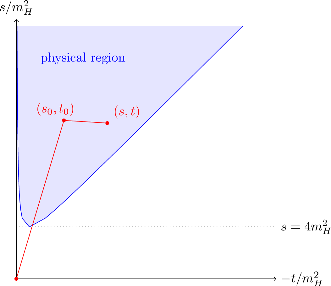
To evaluate the independent functions numerically in the physical region, we solve their differential equations using DiffExp[57]. As an integration path, we choose two straight segments, as schematically shown in Fig. 3. The first segment connects the large mass limit to a reference point in the physical
region, \[\begin{align} \left\{s_0, t_0, u_0, m_{H,0}^2, m_{W/Z,0}^2\right\} = \left\{\frac{3125}{256}, - \frac{1875}{512}, - \frac{1875}{512}, \frac{625}{256}, 1\right\}\, .
\end{align}\] This part of the path is evaluated once and cross-checked against AMFlow[58], [59]. The reference point is then used as a starting point for the second segment to explore the physical region.
This split of the integration path ensures that all kinematic thresholds, which lie outside the physical region and may otherwise slow down the numerical integration, are crossed only once during the evaluation of the reference point.
Figure 3: Schematic illustration of the integration path used to evaluate the independent functions.
The amplitude can be evaluated in this way with a precision of \(16\) significant digits in approximately \(\mathcal{O}(1')\) per phase space point. As this is not sufficiently fast
for a direct implementation into \(\texttt{POWHEG-BOX-V2}\)[60]–[62], we construct an interpolation grid comprising \(\mathcal{O}(20\, 000)\) phase-space points. Therefore, we compute a rectilinear grid in the parameters \[\begin{align} \beta = \sqrt{1 - 4\, \frac{m_H^2}{s}} \in [0,1[ \quad\text{and}\quad\cos\theta = \frac{t - u}{s\, \beta} \in [-1, 1]\,,
\end{align}\] with a sampling density weighted according to the amplitude squared.
The LO amplitudes as well as the real-emission contributions are evaluated on the fly using GoSam-3.
We calculate differential distributions for a center-of-mass energy of \(\sqrt{S} = 13.6\,\mathrm{TeV}\) using the EW input parameters listed in Tab. 1. The renormalisation and factorisation
scales are chosen dynamically as \(m_{HH}/2\), where \(m_{HH}\) denotes the invariant mass of the Higgs boson pair. The scale uncertainties are estimated through 7-point scale
variations.
Table 1: EW input parameters used for phenomenological results.
\(m_H\) [GeV]
\(m_W\) [GeV]
\(m_Z\) [GeV]
\(G_F\) [GeV\(^{-2}\)]
\(125\)
\(80.36\)
\(91.1876\)
\(0.116639\times10^{-4}\)
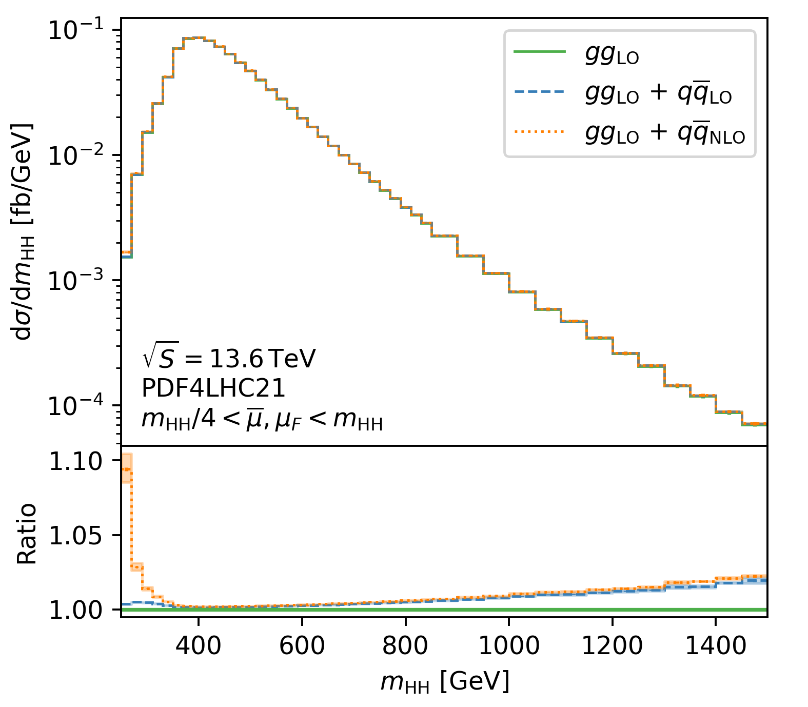
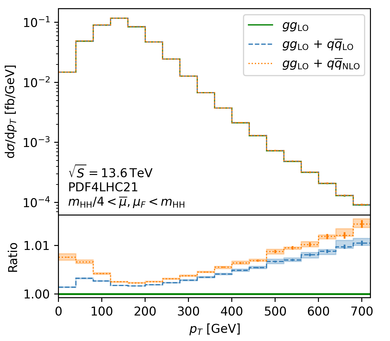
Figure 4: Invariant mass distribution of the Higgs boson pair (a) and transverse momentum distribution of a single Higgs boson (b). The error bands represent the scale uncertainty, while the error bars show the statistical error from the
Monte Carlo simulation..
Fig. 4 (a) shows the invariant mass distribution of the Higgs boson pair. The LO and NLO quark–antiquark contributions are shown as dashed blue and dotted orange lines, respectively, together with the LO gluon-fusion
channel, represented by the solid green line. The NLO quark–antiquark channel exhibits a significant enhancement close to the production threshold, reaching a relative correction of approximately \(+10\%\) compared to LO
gluon-fusion. This effect is mainly driven by real-emissions, since the emitted parton softens the spectrum, which leads to a higher population of the threshold region. At larger invariant masses, the NLO corrections remain positive and reach approximately
\(+3\%\).
Fig. 4 (b) shows the transverse-momentum distribution of one of the Higgs bosons. The corrections exhibit a pattern similar to that observed for the invariant-mass distribution: An enhancement at low transverse momentum,
predominantly driven by real-emission contributions, and a moderate increase in the high-\(p_T\) tail.
These proceedings reviewed the calculation of the quark–antiquark channel for Higgs boson pair production up to NLO QCD. The amplitudes were computed analytically, using differential equations to express Feynman integrals in terms of iterated integrals
over logarithmic kernels. Boundary conditions were obtained from a large-mass expansion, and additional basis rotations were performed to construct a basis of graded transcendental functions. The resulting amplitudes were evaluated on a grid using
DiffExp and implemented into POWHEG-BOX for phenomenological studies.
We observe that the quark–antiquark channel has a sizeable impact on differential distributions, even though its contribution to the total cross section is negligible. In particular, the invariant-mass distribution of the Higgs boson pair shows an
enhancement of nearly \(+10\%\) in the threshold region, as well as noticeable Sudakov-type effects at high energies.
Future work includes the public release of the POWHEG implementation and a detailed study of the interplay between additional EW and QCD contributions to Higgs boson pair production.
This work is supported by the Deutsche Forschungsgemeinschaft (DFG, German Research Foundation) under grant no. - TRR 257, and by the Leverhulme Trust, LIP-2021-014.
G. Aad et al., “Combination of ATLAS and CMS searches for Higgs boson pair production at \(\sqrt{s} = 13\)
TeV,” Feb. 2026, [Online]. Available: https://arxiv.org/abs/2602.23991.
[2]
S. Borowka et al., [Erratum: Phys.Rev.Lett. 117, 079901 (2016)]“Higgs Boson Pair Production in Gluon Fusion at Next-to-Leading Order with Full
Top-Quark Mass Dependence,”Phys. Rev. Lett., vol. 117, no. 1, p. 012001, 2016, doi: 10.1103/PhysRevLett.117.079901.
[3]
S. Borowka et al., “Full top quark mass dependence in Higgs boson pair production at NLO,”JHEP, vol. 10, p. 107, 2016, doi: 10.1007/JHEP10(2016)107.
[4]
J. Baglio, F. Campanario, S. Glaus, M. Mühlleitner, M. Spira, and J. Streicher, “Gluon fusion into Higgs pairs at NLO QCD and the top mass
scheme,”Eur. Phys. J. C, vol. 79, no. 6, p. 459, 2019, doi: 10.1140/epjc/s10052-019-6973-3.
[5]
J. Davies et al., “Double Higgs boson production at NLO: combining the exact numerical result and high-energy expansion,”JHEP,
vol. 11, p. 024, 2019, doi: 10.1007/JHEP11(2019)024.
[6]
J. Baglio et al., “Higgs-Pair Production via Gluon Fusion at Hadron Colliders: NLO QCD Corrections,”JHEP, vol. 4, p. 181, 2020,
doi: 10.1007/JHEP04(2020)181.
[7]
G. Heinrich, S. P. Jones, M. Kerner, G. Luisoni, and E. Vryonidou, “NLO predictions for Higgs boson pair production with full top quark mass dependence matched
to parton showers,”JHEP, vol. 8, p. 088, 2017, doi: 10.1007/JHEP08(2017)088.
[8]
S. Jones and S. Kuttimalai, “Parton Shower and NLO-Matching uncertainties in Higgs Boson Pair Production,”JHEP, vol. 2, p. 176, 2018,
doi: 10.1007/JHEP02(2018)176.
[9]
G. Heinrich, S. P. Jones, M. Kerner, G. Luisoni, and L. Scyboz, “Probing the trilinear Higgs boson coupling in di-Higgs production at NLO QCD including parton
shower effects,”JHEP, vol. 6, p. 066, 2019, doi: 10.1007/JHEP06(2019)066.
[10]
E. Bagnaschi, G. Degrassi, and R. Gröber, “Higgs boson pair production at NLO in the POWHEG approach and the top quark mass uncertainties,”Eur. Phys. J. C, vol. 83, no. 11, p. 1054, 2023, doi: 10.1140/epjc/s10052-023-12238-8.
[11]
J. Davies, K. Schönwald, M. Steinhauser, and D. Stremmer, “ggxy: A flexible library to compute gluon-induced cross sections,”Comput. Phys.
Commun., vol. 320, p. 109933, 2026, doi: 10.1016/j.cpc.2025.109933.
[12]
S. Alioli, G. Marinelli, and D. Napoletano, “NNLO+PS double Higgs boson production with top-quark mass corrections in GENEVA,”JHEP,
vol. 9, p. 206, 2025, doi: 10.1007/JHEP09(2025)206.
[13]
M. Grazzini et al., “Higgs boson pair production at NNLO with top quark mass effects,”JHEP, vol. 5, p. 059, 2018, doi: 10.1007/JHEP05(2018)059.
[14]
D. de Florian et al., “Differential Higgs Boson Pair Production at Next-to-Next-to-Leading Order in QCD,”JHEP, vol. 9, p. 151,
2016, doi: 10.1007/JHEP09(2016)151.
[15]
J. Grigo, J. Hoff, and M. Steinhauser, “Higgs boson pair production: top quark mass effects at NLO and NNLO,”Nucl. Phys. B, vol. 900,
pp. 412–430, 2015, doi: 10.1016/j.nuclphysb.2015.09.012.
[16]
L.-B. Chen, H. T. Li, H.-S. Shao, and J. Wang, “Higgs boson pair production via gluon fusion at N\(^3\)LO in
QCD,”Phys. Lett. B, vol. 803, p. 135292, 2020, doi: 10.1016/j.physletb.2020.135292.
[17]
L.-B. Chen, H. T. Li, H.-S. Shao, and J. Wang, “The gluon-fusion production of Higgs boson pair: N\(^3\)LO QCD corrections and
top-quark mass effects,”JHEP, vol. 3, p. 072, 2020, doi: 10.1007/JHEP03(2020)072.
[18]
A. A H and H.-S. Shao, “N\(^{3}\)LO+N\(^{3}\)LL QCD improved Higgs pair cross
sections,”JHEP, vol. 2, p. 067, 2023, doi: 10.1007/JHEP02(2023)067.
[19]
J. Baglio, F. Campanario, S. Glaus, M. Mühlleitner, J. Ronca, and M. Spira, “\(gg\to HH\) : Combined
uncertainties,”Phys. Rev. D, vol. 103, no. 5, p. 056002, 2021, doi: 10.1103/PhysRevD.103.056002.
[20]
S. Jaskiewicz, S. Jones, R. Szafron, and Y. Ulrich, “The structure of quark mass corrections in the gg HH amplitude at
high-energy,”JHEP, vol. 9, p. 015, 2025, doi: 10.1007/JHEP09(2025)015.
[21]
J. Davies, K. Schönwald, and M. Steinhauser, “Three-loop large-N\(_{c}\) virtual corrections to gg HH in the
forward limit,”JHEP, vol. 8, p. 192, 2025, doi: 10.1007/JHEP08(2025)192.
[22]
H.-Y. Bi, L.-H. Huang, R.-J. Huang, Y.-Q. Ma, and H.-M. Yu, “Electroweak Corrections to Double Higgs Production at the LHC,”Phys. Rev.
Lett., vol. 132, no. 23, p. 231802, 2024, doi: 10.22323/1.478.0120.
[23]
S. Borowka, C. Duhr, F. Maltoni, D. Pagani, A. Shivaji, and X. Zhao, “Probing the scalar potential via double Higgs boson production at hadron
colliders,”JHEP, vol. 4, p. 016, 2019, doi: 10.1007/JHEP04(2019)016.
[24]
M. Mühlleitner, J. Schlenk, and M. Spira, “Top-Yukawa-induced corrections to Higgs pair production,”JHEP, vol. 10, p. 185, 2022, doi:
10.1007/JHEP10(2022)185.
[25]
J. Davies, G. Mishima, K. Schönwald, M. Steinhauser, and H. Zhang, “Higgs boson contribution to the leading two-loop Yukawa corrections to gg
HH,”JHEP, vol. 8, p. 259, 2022, doi: 10.1007/JHEP08(2022)259.
[26]
J. Davies, K. Schönwald, M. Steinhauser, and H. Zhang, “Next-to-leading order electroweak corrections to \(gg \to HH\) and
\(gg \to gH\) in the large-\(m_t\) limit,”JHEP, vol. 10, p. 033, 2023, doi: 10.1007/JHEP10(2023)033.
[27]
W. Bizoń, U. Haisch, L. Rottoli, Z. Gillis, B. Moser, and P. Windischhofer, “Addendum to: Constraints on the quartic Higgs self-coupling from double-Higgs
production at future hadron colliders [JHEP 10 (2019) 267],”JHEP, vol. 2, p. 170, 2024, doi: 10.1007/JHEP02(2024)170.
[28]
G. Heinrich, S. Jones, M. Kerner, T. Stone, and A. Vestner, “Electroweak corrections to Higgs boson pair production: the top-Yukawa and self-coupling
contributions,”JHEP, vol. 11, p. 040, 2024, doi: 10.1007/JHEP11(2024)040.
[29]
J. Davies, K. Schönwald, M. Steinhauser, and H. Zhang, “Analytic next-to-leading order Yukawa and Higgs boson self-coupling corrections to gg HH
at high energies,”JHEP, vol. 4, p. 193, 2025, doi: 10.1007/JHEP04(2025)193.
[30]
M. Bonetti, P. Rendler, and W. J. Torres Bobadilla, “Two-loop light-quark Electroweak corrections to Higgs boson pair production in gluon
fusion,”JHEP, vol. 7, p. 024, 2025, doi: 10.1007/JHEP07(2025)024.
[31]
A. Bhattacharya et al., “Higgs-Pair Production via Gluon Fusion: Top-Yukawa- and light-quark-induced electroweak Corrections,” Dec.
2025, [Online]. Available: https://arxiv.org/abs/2512.14823.
[32]
J. Davies, K. Schönwald, M. Steinhauser, and H. Zhang, “Analytic next-to-leading order electroweak corrections to Higgs boson pair production at high
energies,” Mar. 2026, [Online]. Available: https://arxiv.org/abs/2603.08789.
[33]
M. Bonetti, G. Heinrich, P. Rendler, and W. J. Torres Bobadilla, “NLO QCD corrections to the electroweak production of a Higgs boson pair in the
quark-antiquark channel,”JHEP, vol. 4, p. 131, 2026, doi: 10.1007/JHEP04(2026)131.
[34]
G. Cullen et al., “Automated One-Loop Calculations with GoSam,”Eur. Phys. J. C, vol. 72, p. 1889, 2012, doi: 10.1140/epjc/s10052-012-1889-1.
[35]
G. Cullen et al., “G\(\scriptsize{O}\)S\(\scriptsize{AM}\)-2.0: a tool for automated
one-loop calculations within the Standard Model and beyond,”Eur. Phys. J. C, vol. 74, no. 8, p. 3001, 2014, doi: 10.1140/epjc/s10052-014-3001-5.
[36]
J. Braun et al., “One-loop calculations in effective field theories with GoSam-3.0,”SciPost Phys. Codeb., vol. 62, p. 1, 2026,
doi: 10.21468/SciPostPhysCodeb.62.
[37]
P. Nogueira, “Automatic Feynman Graph Generation,”J. Comput. Phys., vol. 105, pp. 279–289, 1993, doi: 10.1006/jcph.1993.1074.
[38]
J. Davies, T. Kaneko, C. Marinissen, T. Ueda, and J. A. M. Vermaseren, “FORM Version 5.0,” Jan. 2026, [Online]. Available: https://arxiv.org/abs/2601.19982.
J. C. Romao and J. P. Silva, “A resource for signs and Feynman diagrams of the Standard Model,”Int. J. Mod. Phys. A, vol. 27, p.
1230025, 2012, doi: 10.1142/S0217751X12300256.
[41]
M. S. Chanowitz, M. Furman, and I. Hinchliffe, “The Axial Current in Dimensional Regularization,”Nucl. Phys. B, vol. 159, pp. 225–243,
1979, doi: 10.1016/0550-3213(79)90333-X.
[42]
A. von Manteuffel and C. Studerus, “Reduze 2 - Distributed Feynman Integral Reduction,” Jan. 2012, [Online]. Available: https://arxiv.org/abs/1201.4330.
[43]
P. Maierhöfer, J. Usovitsch, and P. Uwer, “KiraA Feynman integral reduction program,”Comput. Phys. Commun., vol. 230, pp.
99–112, 2018, doi: 10.1016/j.cpc.2018.04.012.
[44]
J. Klappert and F. Lange, “Reconstructing rational functions with FireFly,”Comput. Phys. Commun., vol. 247, p. 106951, 2020, doi: 10.1016/j.cpc.2019.106951.
[45]
J. Klappert, F. Lange, P. Maierhöfer, and J. Usovitsch, “Integral reduction with Kira 2.0 and finite field methods,”Comput. Phys.
Commun., vol. 266, p. 108024, 2021, doi: 10.1016/j.cpc.2021.108024.
[46]
J. Klappert, S. Y. Klein, and F. Lange, “Interpolation of dense and sparse rational functions and other improvements in FireFly,”Comput.
Phys. Commun., vol. 264, p. 107968, 2021, doi: 10.1016/j.cpc.2021.107968.
[47]
F. Lange, J. Usovitsch, and Z. Wu, “Kira 3: integral reduction with efficient seeding and optimized equation selection,”Comput. Phys.
Commun., vol. 322, p. 109999, 2026, doi: 10.1016/j.cpc.2025.109999.
[48]
J. M. Henn, “Multiloop integrals in dimensional regularization made simple,”Phys. Rev. Lett., vol. 110, p. 251601, 2013, doi: 10.1103/PhysRevLett.110.251601.
[49]
J. Henn, B. Mistlberger, V. A. Smirnov, and P. Wasser, “Constructing d-log integrands and computing master integrals for three-loop four-particle
scattering,”JHEP, vol. 4, p. 167, 2020, doi: 10.1007/JHEP04(2020)167.
[50]
W. Flieger and W. J. Torres Bobadilla, “Landau and leading singularities in arbitrary space-time dimensions,”Eur. Phys. J. Plus, vol.
139, no. 11, p. 1022, 2024, doi: 10.1140/epjp/s13360-024-05796-7.
[51]
R. N. Lee, “Presenting LiteRed: a tool for the Loop InTEgrals REDuction,” Dec. 2012, [Online]. Available: https://arxiv.org/abs/1212.2685.
[52]
T. Peraro, “\(\text{FiniteFlow}\): multivariate functional reconstruction using finite fields and dataflow
graphs,”JHEP, vol. 7, p. 031, 2019, doi: 10.1007/JHEP07(2019)031.
[53]
A. Matijašić and J. Miczajka, unpublished“Effortless: Efficient generation of odd letters with multiple roots as leading singularities,” In preparation.
[54]
D. Chicherin, V. Sotnikov, and S. Zoia, “Pentagon functions for one-mass planar scattering amplitudes,”JHEP, vol. 1, p. 096, 2022, doi:
10.1007/JHEP01(2022)096.
[55]
T. Gehrmann et al., “Graded transcendental functions: an application to four-point amplitudes with one off-shell leg,”JHEP,
vol. 12, p. 215, 2024, doi: 10.1007/JHEP12(2024)215.
[56]
S. Catani, “The Singular behavior of QCD amplitudes at two loop order,”Phys. Lett. B, vol. 427, pp. 161–171, 1998, doi: 10.1016/S0370-2693(98)00332-3.
[57]
M. Hidding, “DiffExp, a Mathematica package for computing Feynman integrals in terms of one-dimensional series expansions,”Comput. Phys.
Commun., vol. 269, p. 108125, 2021, doi: 10.1016/j.cpc.2021.108125.
[58]
X. Liu, Y.-Q. Ma, and C.-Y. Wang, “A Systematic and Efficient Method to Compute Multi-loop Master Integrals,”Phys. Lett. B, vol. 779,
pp. 353–357, 2018, doi: 10.1016/j.physletb.2018.02.026.
[59]
X. Liu and Y.-Q. Ma, “AMFlow: A Mathematica package for Feynman integrals computation via auxiliary mass flow,”Comput. Phys. Commun.,
vol. 283, p. 108565, 2023, doi: 10.1016/j.cpc.2022.108565.
[60]
P. Nason, “A New method for combining NLO QCD with shower Monte Carlo algorithms,”JHEP, vol. 11, p. 040, 2004, doi: 10.1088/1126-6708/2004/11/040.
[61]
S. Frixione, P. Nason, and C. Oleari, “Matching NLO QCD computations with Parton Shower simulations: the POWHEG method,”JHEP, vol. 11,
p. 070, 2007, doi: 10.1088/1126-6708/2007/11/070.
[62]
S. Alioli, P. Nason, C. Oleari, and E. Re, “A general framework for implementing NLO calculations in shower Monte Carlo programs: the POWHEG
BOX,”JHEP, vol. 6, p. 043, 2010, doi: 10.1007/JHEP06(2010)043.
Note, that FORM 5.0 has since become available [38].↩︎