From Cosmological Cuts to Yang–Mills Wavefunctions in de Sitter Space
June 24, 2026
UTF8gbsn
1 Introduction↩︎
Cosmological unitarity gives direct access to the singularity structure of the Bunch–Davies wavefunction and related observables. A central result is the cosmological optical theorem, which relates wavefunction coefficients to their Hermitian-analytic images [1]–[4]. For exchange diagrams, these relations expose the same physical information that one would like to use recursively: a singularity in an internal energy factorizes the observable into lower-point data.
This factorization naturally supports reconstruction approaches to cosmological observables. Locality and unitarity restrict the allowed total- and partial-energy singularities, and in favorable cases these singularities reconstruct rational wavefunction or correlator data from lower-point or flat-space input [5]–[7]. Discontinuities also enter directly in recent single-cut, Schwinger–Keldysh, dispersive, physical-cut-basis, and dressing-rule approaches to cosmological correlators [8]–[16]. In this paper we use such singularity data constructively: the cuts are not only checks on an answer, but input for reconstructing the wavefunction.
For spinning fields, the general cutting rules are known, but explicit high-point implementations are still scarce. General bosonic formulas imply tree-level factorization for exchanges of arbitrary integer spin [2], [4]; the practical problem is to turn this factorization into usable reconstruction rules. Yang–Mills theory is a useful test case because nontrivial tensor structures already appear at low multiplicity. Related bootstrap constructions, factorization analyses, AdS recursion relations, soft theorems, and amplitude-inspired representations in \((A)dS\) provide complementary ways of organizing the same class of observables [17]–[22].
There is also a useful analogy with flat-space amplitudes. In flat-space scattering, sufficiently sharp cuts isolate rigid data: generalized cuts and leading singularities constrain loop integrands, while on-shell diagrams organize such residues in terms of cells of the positive Grassmannian [23]–[28]. This viewpoint is intertwined with positive-geometric structures such as the amplituhedron, positive geometries and canonical forms, kinematic associahedra and scattering forms, and more recent surface-based organizations of amplitudes [29]–[36]. Cosmological observables have their own geometric and combinatorial structures, including cosmological polytopes, scattering facets, Steinmann-type compatibility constraints, cosmohedra, and correlator polytopes [37]–[42]. The analogy is not literal, because cosmological wavefunctions have a different analytic structure from flat-space amplitudes [43]–[45]. Still, it suggests a concrete question: how much of a spinning cosmological wavefunction is already fixed by the most restrictive discontinuities?
The aim of this paper is to make the discontinuity-based reconstruction of tree-level Yang–Mills de Sitter wavefunctions explicit in momentum space. Closely related ideas have been used to bootstrap four- and five-point gluon and graviton wavefunctions in Mellin-momentum space [46], [47]. Here we formulate the gluing rule for gluon discontinuities, turn it into a reconstruction procedure, and work out the four-, five-, and six-point wavefunction coefficients in momentum space. The maximal discontinuities play the role of cosmological leading singularities, while lower-codimension cuts supply the remaining gluing data. The explicit answers separate into a cut-detectable part and a smaller cut-invisible completion fixed by current conservation, and the flat-space limit. We check the reconstruction against direct Yang–Mills momentum-space Feynman rules and use the low-point results to identify the first ingredients of an all-\(n\) organization. Section 3.2 gives the reconstruction strategy; the four-, five-, and six-point cases are then treated in Sections 3.3–3.5, before the all-\(n\) pattern is summarized in Section 3.6.
Notation and conventions
Throughout the paper we write \[k_a:=|\boldsymbol{k}_a|\] for the external energies. When a subset of external momenta is separated by an internal channel \(I\), we denote the corresponding exchanged spatial momentum and energy by \[\boldsymbol{k}_I := \sum_{a\in I}\boldsymbol{k}_a, \qquad k_I := |\boldsymbol{k}_I| .\] For ordered planar channels it is useful to use the shorthand \[x_{ij}:=\left|\boldsymbol{k}_i+\boldsymbol{k}_{i+1}+\cdots+\boldsymbol{k}_{j-1}\right|=k_{\underline{i\,i+1\cdots j-1}}, \qquad i<j,\] so that, for example, \(x_{13}=|\boldsymbol{k}_1+\boldsymbol{k}_2|\). We also denote the \(n\)-point total energy by \[E_n:=\sum_{a=1}^{n}k_a=k_1+k_2+\cdots+k_n .\]
We work in \(\mathrm{dS}_4\), with metric \[ds_{\mathrm{dS}}^2 = \frac{\ell_{\mathrm{dS}}^2}{\eta^2} \left( -d\eta^2+\delta_{ij}dx^i dx^j \right). \label{eq:ds-metric}\tag{1}\] Here \(\eta\in(-\infty,\eta_\ast)\) is conformal time, and \(\eta_\ast\to0^-\) is the late-time cutoff at which the wavefunction is evaluated. We set \(H=1/\ell_{\mathrm{dS}}=1\) in the following.
In practice, it is convenient to compute the corresponding diagrams in Euclidean \(\mathrm{AdS}_4\), \[ds_{\mathrm{EAdS}}^2 = \frac{\ell_{\mathrm{AdS}}^2}{z^2} \left( dz^2+\delta_{ij}dx^i dx^j \right),\] and then analytically continue \[z=-i\eta,\qquad z_\ast=-i\eta_\ast,\qquad \ell_{\mathrm{AdS}}^2=-\ell_{\mathrm{dS}}^2 .\] Equivalently, one may choose the branch \(\ell_{\mathrm{AdS}}=-i\ell_{\mathrm{dS}}\). With these continuations the Euclidean \(\mathrm{AdS}\) metric maps to the Lorentzian \(\mathrm{dS}\) metric above [48]–[50].
2 Review of wavefunction coefficients and cutting rules↩︎
This section fixes the conventions used in the reconstruction. We first recall the late-time Bunch–Davies wavefunction coefficients, then review the energy-sign-flip discontinuity for tree-level rational wavefunctions. We finally specialize the cutting rule to gluons, where the sum over exchanged physical states is implemented by a transverse projector.
2.1 Wavefunction coefficients↩︎
Let \(\Phi(\eta,\mathbf{x})\) denote a bulk field in \(\mathrm{dS}_4\), and let \(\varphi(\mathbf{x})\) be its late-time boundary value, \[\varphi(\mathbf{x})=\Phi(\eta_\ast,\mathbf{x}), \qquad \eta_\ast\to 0^- . \label{eq:boundary-field}\tag{2}\] We work with the late-time wavefunction \(\Psi[\varphi]\), viewed as a functional of the boundary configuration \(\varphi(\mathbf{x})\): \[\Psi[\varphi] = \langle \varphi,\eta_\ast|\, U\!\left(\eta_\ast,-\infty\right) |\Omega_{\rm BD}\rangle , \label{eq:wavefunction-operator}\tag{3}\] where \(|\varphi,\eta_\ast\rangle\) is the field eigenstate at the late-time slice, \(|\Omega_{\rm BD}\rangle\) is the Bunch–Davies initial state, and \(U\) is the time-evolution operator from the deformed past contour to \(\eta_\ast\). In the path-integral representation this becomes \[\Psi[\varphi] = \int_{\Phi(\eta\to-\infty,\mathbf{x})=0} ^{\Phi(\eta_\ast,\mathbf{x})=\varphi(\mathbf{x})} \mathcal{D}\Phi\, \exp\!\left(\mathrm{i}S[\Phi]\right). \label{eq:wavefunction-path-integral}\tag{4}\] Here the lower endpoint of the time contour is deformed as \(-\infty \to -\infty(1-\mathrm{i}\epsilon)\). This is the standard prescription implementing the Bunch–Davies initial condition in the asymptotic past [1], [2], [43], [48], [51].
From now on, we work in momentum space and allow for a collection of boundary fields \(\varphi_\alpha(\boldsymbol{k})\), where the label \(\alpha\) denotes the field species and, when appropriate, any discrete external-state labels such as color or helicity. Since the wavefunction is a functional of these boundary fields, it admits the perturbative functional Taylor expansion \[\require{physics} \begin{align} \Psi[\varphi_\alpha] = \exp \Bigg[ -\sum_{n=2}^{\infty} \frac{1}{n!} \sum_{\alpha_1,\ldots,\alpha_n} \int \prod_{a=1}^{n} \frac{\dd^3\boldsymbol{k}_a}{(2\pi)^3}\, (2\pi)^3 \delta^{(3)} \!\left(\sum_{a=1}^{n}\boldsymbol{k}_a\right) \psi_n^{\alpha_1\cdots\alpha_n}(\boldsymbol{k}_1,\ldots,\boldsymbol{k}_n) \prod_{a=1}^{n}\varphi_{\alpha_a}(\boldsymbol{k}_a) \Bigg]. \label{eq:wavefunction-momentum} \end{align}\tag{5}\] Here \(\varphi_\alpha(\boldsymbol{k})\) is the Fourier transform of the boundary field, and \(\psi_n^{\alpha_1\cdots\alpha_n}\) is the momentum-conserving-delta-function-stripped \(n\)-point coefficient, evaluated on \(\sum_{a=1}^n \boldsymbol{k}_a=0\). These coefficients are constrained by the conformal symmetry of the late-time boundary and can be computed by analytic continuation from AdS Witten diagrams [5], [48]–[50], [52]–[54]. For gluons, one also sums over color and helicity states.
The corresponding color-dressed coefficient can be decomposed in a trace basis as \[\require{physics} \psi_n^{a_1\cdots a_n;\,h_1\cdots h_n} (\boldsymbol{k}_1,\ldots,\boldsymbol{k}_n) = \sum_{\sigma\in S_n/\mathbb{Z}_n} \Tr\!\left( T^{a_{\sigma(1)}}\cdots T^{a_{\sigma(n)}} \right) \psi_n\!\left[ \sigma(1)^{h_{\sigma(1)}},\ldots, \sigma(n)^{h_{\sigma(n)}} \right]. \label{eq:gluon-trace-basis}\tag{6}\] Here \(\psi_n[\sigma(1)^{h_{\sigma(1)}},\ldots, \sigma(n)^{h_{\sigma(n)}}]\) is the color-ordered gluon wavefunction coefficient. It no longer carries explicit color indices, but depends on the ordering, helicities, momenta, and energies.
In this work we focus on the color-ordered, polarization-contracted, transverse part of the gluon wavefunction coefficient. The helicity of each external gluon is carried by its polarization vector, and we write \(\boldsymbol{\epsilon}_a\equiv\boldsymbol{\epsilon}_a^{h_a}(\boldsymbol{k}_a)\) while leaving the helicity labels implicit throughout: \[\psi_n^{\mathrm{YM}} \bigl( \{\boldsymbol{\epsilon}_a,\boldsymbol{k}_a,k_a\}_{a=1}^{n} \bigr) := \boldsymbol{\epsilon}_1^{i_1}\cdots \boldsymbol{\epsilon}_n^{i_n}\, \psi^{\mathrm{YM}}_{n;i_1\cdots i_n} \bigl( \boldsymbol{k}_1,\ldots,\boldsymbol{k}_n \bigr), \label{eq:ym-contracted-wavefunction}\tag{7}\] The external polarizations satisfy \[\boldsymbol{\epsilon}_a\cdot\boldsymbol{k}_a=0, \qquad a=1,\ldots,n .\] This transverse, polarization-contracted object is the basic quantity whose discontinuities we study and whose full form we later reconstruct. The longitudinal components of the full Yang–Mills wavefunction coefficient are fixed by the transverse Ward identities [50], [55], [56].
2.2 Cutting rules and discontinuities↩︎
The cosmological optical theorem constrains Hermitian-analytic discontinuities of wavefunction coefficients. The associated cutting rules relate these discontinuities, defined by subtracting the corresponding Hermitian-analytic image, to products of lower-point data [1], [2], [4], [6], [7].
We will use the same discontinuities as reconstruction data. The basic mechanism is already visible at the level of a single internal bulk-to-bulk propagator: its discontinuity separates an exchange diagram into lower-point wavefunction or correlator data. Conversely, such factorized data can be used as input for dispersive or cut-based reconstruction of full wavefunctions and correlators [3], [10], [11], [13], [16], [57], [58]. In this paper we focus on wavefunction coefficients.
It is convenient to record the spectral representation here: \[G_{\Delta}(k,z_1,z_2) = -i\int_{0}^{\infty}\frac{dp}{2\pi i}\, \frac{p^{d+1-2\Delta}}{k^2+p^2} \bigl(\phi_{\Delta}(z_1,ip)-\phi_{\Delta}(z_1,-ip)\bigr) \bigl(\phi_{\Delta}(z_2,ip)-\phi_{\Delta}(z_2,-ip)\bigr), \label{eq:btb-spectral-representation}\tag{8}\] where \(\phi_{\Delta}(z,k_I)\) is the corresponding bulk-to-boundary mode.
At tree level, the non-analytic dependence on an internal exchange energy \(k_I\) comes from the corresponding bulk-to-bulk propagator. The factorization across the channel \(I\) is therefore the discontinuity of this Green function. Using the spectral representation gives1 \[\operatorname{Disc}_{k_I^2} G_{\Delta}(z_1,z_2;k_I) = -P_{k_I}\, \bigl[ \phi_{\Delta}(z_1,k_I)-\phi_{\Delta}(z_1,-k_I) \bigr] \bigl[ \phi_{\Delta}(z_2,k_I)-\phi_{\Delta}(z_2,-k_I) \bigr] . \label{eq:btb-propagator-disc}\tag{9}\] Here \(P_{k_I}\) denotes the power spectrum, \(P_{k_I} = \frac{1}{2}k_I^{d-2\Delta}.\) Thus the discontinuity of the bulk-to-bulk propagator factorizes into two bulk-to-boundary differences times the power spectrum.
Diagrammatically, cutting the internal line in channel \(I\) separates the full wavefunction into left and right sub-wavefunction coefficients: \[\operatorname{Disc}_{k_I^2}\psi_n = - (\psi_L(k_I)-\psi_L(-k_I))\; P_I\; ( \psi_R(k_I)-\psi_R(-k_I) ). \label{eq:cutting-rule}\tag{10}\] For the rational functions considered here, the discontinuity of the full wavefunction is given by the difference2 \[\operatorname{Disc}_{k_I^2}F(k_I)=F(k_I)-F(-k_I). \label{signflip}\tag{11}\] In the rest of the text, when no confusion can arise, we write \(\operatorname{Disc}_{k_I^2}F(k_I):=\operatorname{Disc}_{k_I}F(k_I)\).
It is also useful to define iterated discontinuities. Let \(S=\{I_1,\ldots,I_m\}\) be a set of mutually compatible channels. We define \[\operatorname{Disc}_S := \prod_{I\in S}\operatorname{Disc}_{k_I}. \label{eq:iterated-disc-review}\tag{12}\] Compatibility means that the chosen channels can be cut simultaneously and nontrivially on the same tree graph. Repeated use of 10 then decomposes the original wavefunction coefficient into lower-point building blocks glued along all channels in \(S\). In particular, maximal compatible cuts, where every internal channel of a given tree topology is cut, localize the answer as much as possible and will play the role of cosmological analogues of leading singularities in the discussion below.
2.2.1 Flat-space massless trace \(\phi^3\) maximal discontinuities↩︎
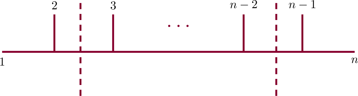
As a simple toy model, consider the flat-space massless trace \(\phi^3\) wavefunction. We start with the scalar cubic three-point building block \[\psi_{3}^{\mathrm{tr}\,\phi^3}(k_1,k_2,k_3) = C_3(k_1,k_2,k_3) := \frac{1}{k_1+k_2+k_3}, \label{eq:scalar-cubic-block}\tag{13}\] where \(k_1,k_2,k_3\) are energies. If one of these arguments is a cut energy, the discontinuity is implemented by the sign flip defined in 11 . For example, \[\begin{align} \operatorname{Disc}_{k_1} C_3(k_1,k_2,k_3) &= C_3(k_1,k_2,k_3)-C_3(-k_1,k_2,k_3) \nonumber\\ &= -\frac{2k_1}{(k_1+k_2+k_3)(-k_1+k_2+k_3)} . \label{eq:single-disc-cubic-block} \end{align}\tag{14}\] Similarly, the double discontinuity in two energy slots is \[\begin{align} & \operatorname{Disc}_{k_1}\operatorname{Disc}_{k_3} C_3(k_1,k_2,k_3)\\ =& C_3(k_1,k_2,k_3) - C_3(k_1,k_2,-k_3) - C_3(-k_1,k_2,k_3) + C_3(-k_1,k_2,-k_3) \nonumber\\ =& \frac{8k_1k_2k_3}{\bigl((k_1+k_2)^2-k_3^2\bigr)\bigl((k_2-k_1)^2-k_3^2\bigr)} . \label{eq:double-disc-cubic-block} \end{align}\tag{15}\] These two elementary expressions are the only scalar ingredients needed for the maximal cuts considered below. The tree half-ladder assignment is illustrated in Fig. 1: endpoint vertices carry one cut channel and therefore one discontinuity, while internal vertices carry two cut channels and therefore a double discontinuity. In a one-loop \(n\)-gon, every cubic vertex is adjacent to two cut loop lines and therefore also carries a double discontinuity, as illustrated in Fig. 2.
2.2.1.1 Tree-level half-ladder.
Consider the color ordering \((1,2,\ldots,n)\). In the notation introduced in the introduction, the internal channels of the half-ladder are \[x_{13},x_{14},\ldots,x_{1,n-1}.\] The maximal discontinuity for this topology is therefore \[\operatorname{Disc}_{\rm max} := \prod_{m=2}^{n-2} \operatorname{Disc}_{x_{1,m+1}} . \label{eq:half-ladder-max-disc-operator}\tag{16}\]
Since each internal bulk-to-bulk propagator is cut according to 10 , applying the maximal discontinuity operator 16 makes the scalar cubic half-ladder factorize vertex by vertex: \[\begin{align} &\operatorname{Disc}_{\rm max} \psi^{\phi^3}_{n,\mathrm{HL}} = \left( \prod_{m=2}^{n-2} \frac{1}{2x_{1,m+1}} \right) \Big[ \operatorname{Disc}_{x_{13}} C_3(k_1,k_2,x_{13}) \Big] \nonumber\\ &\times \left( \prod_{m=3}^{n-2} \operatorname{Disc}_{x_{1m}}\operatorname{Disc}_{x_{1,m+1}} C_3(x_{1m},k_m,x_{1,m+1}) \right) \Big[ \operatorname{Disc}_{x_{1,n-1}} C_3(x_{1,n-1},k_{n-1},k_n) \Big], \label{eq:scalar-half-ladder-max-disc} \end{align}\tag{17}\] where we have used the flat-space massless power spectrum \(P_I=1/(2k_I)\). The product over \(m=3,\ldots,n-2\) is understood to be absent when the range is empty. The first and last brackets correspond to the two endpoint vertices of the half-ladder, while the middle product corresponds to the internal cubic vertices. Using 14 and 15 , this expression becomes a local rational function of the external energies and the half-ladder channel variables \(x_{13},\ldots,x_{1,n-1}\).

2.2.1.2 One-loop \(n\)-gon.
For the one-loop \(n\)-gon we need loop-line energies, which are not among the planar tree-channel variables \(x_{ij}\). Let \(\boldsymbol{\ell}\) be the loop spatial momentum and define \[q_0(\boldsymbol{\ell}):=|\boldsymbol{\ell}|, \qquad q_a(\boldsymbol{\ell}) := \left| \boldsymbol{\ell}+\boldsymbol{k}_1+\cdots+\boldsymbol{k}_a \right|, \qquad a=1,\ldots,n . \label{eq:loop-line-energies}\tag{18}\] Momentum conservation gives \(q_n(\boldsymbol{\ell})=q_0(\boldsymbol{\ell})\). Below we suppress the explicit \(\boldsymbol{\ell}\)-dependence and simply write \(q_a\). The \(a\)-th cubic vertex is adjacent to the two cut loop energies \(q_{a-1}\) and \(q_a\), with the cyclic identification \(q_n\equiv q_0\).
The scalar maximal-discontinuity integrand is then \[\begin{align} \operatorname{Disc}_{\rm max} \mathcal{I}^{\phi^3}_{n,n\text{-}\mathrm{gon}} (\boldsymbol{\ell}) = \left( \prod_{a=0}^{n-1} \frac{1}{2q_a} \right) \left( \prod_{a=1}^{n} \operatorname{Disc}_{q_{a-1}}\operatorname{Disc}_{q_a} C_3(q_{a-1},k_a,q_a) \right), \qquad q_n\equiv q_0 . \label{eq:scalar-ngon-max-disc-integrand} \end{align}\tag{19}\] The full scalar one-loop maximal discontinuity is obtained by integrating over the loop spatial momentum, \[\require{physics} \operatorname{Disc}_{\rm max} \psi^{\phi^3}_{n,n\text{-}\mathrm{gon}} = \int \frac{\dd^3\boldsymbol{\ell}}{(2\pi)^3}\, \operatorname{Disc}_{\rm max} \mathcal{I}^{\phi^3}_{n,n\text{-}\mathrm{gon}} (\boldsymbol{\ell}). \label{eq:scalar-ngon-max-disc}\tag{20}\] These scalar expressions will serve as the energy factors that are dressed by Yang–Mills tensor numerators in the ray-like tree and one-loop \(n\)-gon examples below.
2.3 Discontinuities of gluon wavefunction coefficients↩︎
For the reader’s convenience, we record the Yang–Mills bulk-to-boundary and bulk-to-bulk propagators here. The bulk-to-boundary propagator is \[\label{eq:ym-btb-propagator} \phi^i(z,k)\equiv\boldsymbol{\epsilon}^i \phi(z,k)=\boldsymbol{\epsilon}^i e^{-zk},\tag{21}\] while the transverse bulk-to-bulk propagator is written in spectral form as \[\label{eq:ym-transverse-btb-spectral} \begin{align} G^\perp_{ij}(z_1,z_2;k_I) &= -\frac{1}{4}\Pi_{ij}^{(\boldsymbol{k}_I)} \int_{-\infty}^{\infty}\frac{dp}{\pi}\, \frac{(\phi(z_1,ip)-\phi(z_1,-ip))(\phi(z_2,ip)-\phi(z_2,-ip))}{k_I^2+p^2}, \end{align}\tag{22}\] where \(\Pi_{ij}^{(\boldsymbol{k}_I)} = \delta_{ij} -\frac{\boldsymbol{k}_I^i \boldsymbol{k}_I^j}{k_I^2}.\) The longitudinal part is analytic in \(k_I\) and does not contribute to the discontinuity considered in this subsection. The scalar part appearing in 21 and 22 is the flat-space massless scalar bulk-to-boundary and bulk-to-bulk propagator [37]. This follows from the conformally coupled nature of Yang–Mills theory in (A)dS.
For Yang–Mills wavefunction coefficients, the scalar discontinuity is dressed by the tensor factor in the propagator. The transverse projector \(\Pi^{ij}(\boldsymbol{k}_I)\) in 22 is analytic in \(k_I\), so it factors out of the energy discontinuity. It is also the helicity sum over the two cut gluon polarizations, \(\sum_h \epsilon_i^{(h)}(\boldsymbol{k}_I)\, \epsilon_j^{(h)\,*}(\boldsymbol{k}_I) = \Pi_{ij}(\boldsymbol{k}_I).\) The right-hand side of 9 is therefore replaced by energy-flipped differences of gluon bulk-to-boundary propagators3 (cf. 21 ).
The single-cut rule becomes \[\begin{align} \operatorname{Disc}_{k_I}\psi_n^{\mathrm{YM}} = P^{\mathrm{YM}}(k_I)\, \Bigg[ \frac{\partial}{\partial \epsilon_I^i} \operatorname{Disc}_{k_I} \psi_L^{\mathrm{YM}} \bigl( \epsilon_I,-\boldsymbol{k}_I,k_I \bigr) \Bigg] \Pi^{ij}(\boldsymbol{k}_I) \Bigg[ \frac{\partial}{\partial \tilde{\epsilon}_I^j} \operatorname{Disc}_{k_I} \psi_R^{\mathrm{YM}} \bigl( \tilde{\epsilon}_I,\boldsymbol{k}_I,k_I \bigr) \Bigg] . \label{eq:ym-single-cut} \end{align}\tag{23}\] Here \(P^{\mathrm{YM}}(k_I)=1/(2k_I)\) is the Yang–Mills power spectrum on the cut line, and \(\Pi^{ij}(\boldsymbol{k}_I)\) performs the helicity sum. The discontinuity \(\operatorname{Disc}_{k_I}\) acts only on the scalar energy dependence, not on the tensor structure. Differentiating with respect to the auxiliary polarizations, \(\frac{\partial}{\partial \epsilon_I^i}, \; \frac{\partial}{\partial \tilde{\epsilon}_I^j},\) strips off the polarization of the lower-point wavefunction coefficient and exposes the vector index to be glued by the projector. Thus the discontinuity in channel \(I\) factorizes into two lower-point discontinuities connected by the physical polarization sum of the exchanged gluon.
For a compatible set of channels \(S\), the iterated Yang–Mills cut is obtained by applying 23 to every channel in \(S\). Let \(\mathcal{C}(\mathcal{T}/S)\) denote the set of connected components obtained from the tree topology \(\mathcal{T}\) after cutting all edges in \(S\). For a component \(C\in\mathcal{C}(\mathcal{T}/S)\), we define \[\mathrm{Inc}(C) := \{\, e\in S \;|\; e \text{ is incident on } C \,\}.\] Thus \(\mathrm{Inc}(C)\) is the set of cut lines attached to the lower-point wavefunction coefficient associated with \(C\). For each incident cut edge \(e\in \mathrm{Inc}(C)\), we introduce an auxiliary polarization \(\epsilon_{e,C}\) on the corresponding cut leg. Differentiating with respect to these auxiliary polarizations opens the vector indices that will be glued to the neighboring components.
With this notation, repeated use of the single-cut rule gives the multi-cut formula \[\begin{align} \operatorname{Disc}_S \psi_n^{\mathrm{YM}} = \left[ \prod_{e\in S} P^{\mathrm{YM}}(k_e) \right] \left[ \prod_{e=(C,C')\in S} \Pi^{\,i_{e,C}i_{e,C'}}(\boldsymbol{k}_e) \right] \prod_{C\in\mathcal{C}(\mathcal{T}/S)} \left[ \left( \prod_{e\in \mathrm{Inc}(C)} \frac{\partial}{\partial \epsilon_{e,C}^{\,i_{e,C}}} \right) \operatorname{Disc}_{\mathrm{Inc}(C)} \psi_C^{\mathrm{YM}} \right] . \label{eq:ym-compatible-cut} \end{align}\tag{24}\] Here \(e=(C,C')\) means that the cut edge \(e\) connects the two components \(C\) and \(C'\). The indices \(i_{e,C}\) and \(i_{e,C'}\) are the open vector indices exposed on the two sides of the cut, and they are contracted by the transverse projector \(\Pi^{\,i_{e,C}i_{e,C'}}(\boldsymbol{k}_e)\). The notation \(\operatorname{Disc}_{\mathrm{Inc}(C)}\) means the product of discontinuities in the cut energies carried by the edges incident on \(C\), \[\operatorname{Disc}_{\mathrm{Inc}(C)} := \prod_{e\in\mathrm{Inc}(C)}\operatorname{Disc}_{k_e}.\]
This formula separates the scalar and spinning data. The cut propagators and discontinuities determine the energy dependence; the tensor structure is built from lower-point Yang–Mills tensors and transverse projectors. We now turn to maximal compatible cuts, where every internal channel of the chosen topology is cut.
2.3.1 Gluon maximal discontinuities↩︎
Among compatible cuts, maximal cuts are the most restrictive: every internal channel of a chosen topology is cut, leaving a local gluing problem. For the ray-like tree (half-ladder) and its one-loop \(n\)-gon analogue, this gives compact closed-form expressions while retaining nontrivial tensor structure.
We begin with the three-point wavefunction coefficient, \[\psi_3(\boldsymbol{\epsilon}_1,\boldsymbol{\epsilon}_2,\boldsymbol{\epsilon}_3;\boldsymbol{k}_1,\boldsymbol{k}_2,\boldsymbol{k}_3;k_1,k_2,k_3) = V_{123}\,C_3(k_1,k_2,k_3). \label{eq:ym-three-point-wavefunction}\tag{25}\] Here the tensor structure is carried by \(V_{123}\), while the scalar part is encoded in the same cubic block \(C_3\) used in the scalar example in Section 2.2.1. Explicitly, \[V_{123} = \boldsymbol{\epsilon}_1^i \boldsymbol{\epsilon}_2^j \boldsymbol{\epsilon}_3^k V_{ijk}(\boldsymbol{k}_1,\boldsymbol{k}_2,\boldsymbol{k}_3) = (\boldsymbol{\epsilon}_1\!\cdot\!\boldsymbol{k}_2)(\boldsymbol{\epsilon}_2\!\cdot\!\boldsymbol{\epsilon}_3) +(\boldsymbol{\epsilon}_1\!\cdot\!\boldsymbol{\epsilon}_3)(\boldsymbol{\epsilon}_2\!\cdot\!\boldsymbol{k}_3) +(\boldsymbol{\epsilon}_1\!\cdot\!\boldsymbol{\epsilon}_2)(\boldsymbol{\epsilon}_3\!\cdot\!\boldsymbol{k}_1).\] Here \(V_{ijk}\) is the three-gluon vertex \[V_{ijk}(\mathbf{p},\mathbf{q},\mathbf{r}) = \frac{1}{2}\left(\delta_{ij}(\mathbf{p}-\mathbf{q})_k +\delta_{jk}(\mathbf{q}-\mathbf{r})_i +\delta_{ki}(\mathbf{r}-\mathbf{p})_j\right).\]
It follows from 24 that the tree-level half-ladder maximal discontinuity is given by \[\operatorname{Disc}_{\max}\psi^{\rm YM}_{n,\mathrm{HL}}(1,\dots,n) = V^{12 i_1}\, \Pi_{i_1 i_2}\, V^{i_2 3 i_3}\, \Pi_{i_3 i_4}\, \cdots\, \Pi_{i_{n-2} i_{n-1}}\, V^{i_{n-1}\, n-1\, n} \operatorname{Disc}_{\rm max} \psi^{\phi^3}_{n,\mathrm{HL}} \, .\] Here \(\operatorname{Disc}_{\rm max} \psi^{\phi^3}_{n,\mathrm{HL}}\) is given in 17 . Thus, the maximal discontinuity of the color-ordered Yang–Mills wavefunction on a ray-like triangulation factorizes into a purely scalar \(\phi^3\) maximal discontinuity times a tensor numerator built by gluing three-point Yang–Mills vertices with transverse projectors.
The same logic extends to the one-loop \(n\)-gon, where the open chain closes into a cyclic trace: \[\require{physics} \operatorname{Disc}_{\max}\psi^{\rm YM}_{n,n\text{-}\mathrm{gon}} = \int\!\frac{\dd^3\boldsymbol{\ell}}{(2\pi)^3}\, V^{i_{n+1}\,1\,i_1}\, \Pi_{i_1 i_2}\, V^{i_2\,2\,i_3}\, \Pi_{i_3 i_4}\, \cdots\, V^{i_n\,n\,i_{n+1}} \operatorname{Disc}_{\max}\mathcal{I}^{\phi^3}_{n,n\text{-}\mathrm{gon}}(\boldsymbol{\ell})\, .\] The scalar integrand appearing here is given in 19 .
Thus, the ray-like tree and its one-loop \(n\)-gon analogue form a particularly clean sector for testing amplitude-inspired organizations of singularity data. At the same time, the cosmological character of the problem remains manifest: the scalar factor is still a cosmological maximal discontinuity rather than an ordinary flat-space leading singularity.
The rest of the section gives a compact recursive formula for the tensor part of the tree and one-loop factorizations, summarized in 33 , and 42 .
2.3.1.1 Local gluing map.
The tensor structure is encoded in a local gluing map built from the three-gluon vertex. Since every maximal-cut formula below is obtained by iterating the same elementary step, it is useful to isolate that step once and for all. We use the all-outgoing convention \[V_{ijk}(p,q,r) = \frac{1}{2}\left(\delta_{ij}(p-q)_k+\delta_{jk}(q-r)_i+\delta_{ki}(r-p)_j\right), \qquad p+q+r=0. \label{eq:ym-vertex}\tag{26}\] Let \(J_i\) be an open current carrying spatial momentum \(P\) and satisfying \(P\!\cdot\!J=0\), and let \(\boldsymbol{\epsilon}_i\) be an external polarization carrying spatial momentum \(k\) with \(k\!\cdot\!\boldsymbol{\epsilon}=0\). We define the single-step gluing map by \[\mathcal{G}_{P,k}[J,\boldsymbol{\epsilon}]_i := \Pi_{ij}(P+k)\,J_m\boldsymbol{\epsilon}_n\,V_{mn}{}^{j}(P,k,-P-k). \label{eq:gluing-map-def}\tag{27}\] A direct contraction gives the explicit form \[\mathcal{G}_{P,k}[J,\boldsymbol{\epsilon}] =\frac{1}{2} \Pi(P+k) \cdot \Big[ (J\!\cdot\!\boldsymbol{\epsilon})(P-k) -2(\boldsymbol{\epsilon}\!\cdot\!P)\,J +2(J\!\cdot\!k)\,\boldsymbol{\epsilon} \Big]. \label{eq:gluing-map}\tag{28}\] In particular, \[(P+k)\cdot \mathcal{G}_{P,k}[J,\boldsymbol{\epsilon}]=0, \label{eq:gluing-transverse}\tag{29}\] so the gluing map preserves transversality. This is the basic local ingredient behind all of the maximal-cut numerators below.
2.3.1.2 Tree-level half-ladder.
Consider the color ordering \((1,2,\dots,n)\) and define the partial momenta \[Q_m:=\boldsymbol{k}_1+\cdots+\boldsymbol{k}_m, \qquad q_m:=|Q_m|, \qquad m=1,\dots,n-1, \label{eq:partial-momenta}\tag{30}\] so that \(q_1=k_1\) and, by momentum conservation, \(Q_{n-1}=-\boldsymbol{k}_n\) and hence \(q_{n-1}=k_n\).
We now define the open current recursively, \[J_1:=\boldsymbol{\epsilon}_1, \qquad J_{1\cdots m} := \mathcal{G}_{Q_{m-1},\,\boldsymbol{k}_m}[J_{1\cdots m-1},\boldsymbol{\epsilon}_m], \qquad m=2,\dots,n-1. \label{eq:current-recursion}\tag{31}\] or, equivalently, \[J_{1\cdots m} = \frac{1}{2}\Pi(Q_m)\Big[ (J_{1\cdots m-1}\!\cdot\!\boldsymbol{\epsilon}_m)(Q_{m-1}-\boldsymbol{k}_m) -2(\boldsymbol{\epsilon}_m\!\cdot\!Q_{m-1})\,J_{1\cdots m-1} +2(J_{1\cdots m-1}\!\cdot\!\boldsymbol{k}_m)\,\boldsymbol{\epsilon}_m \Big]. \label{eq:current-recursion-explicit}\tag{32}\] This makes manifest that each new leg is attached by a single local gluing operation followed by a projection onto the transverse subspace. In particular, the full numerator is built by adjoining one external gluon at a time.
The maximal discontinuity of the Yang–Mills half-ladder then factorizes as \[\operatorname{Disc}_{\max}\psi^{\rm YM}_{n,\mathrm{HL}}(1,\dots,n) = \operatorname{Disc}_{\max}\psi^{\phi^3}_{n,\mathrm{HL}}(1,\dots,n)\, \mathcal{N}^{\mathrm{HL}}_n(1,\dots,n), \label{eq:tree-factorization}\tag{33}\] with tensor factor \[\mathcal{N}^{\mathrm{HL}}_n(1,\dots,n) = \boldsymbol{\epsilon}_n\cdot J_{1\cdots n-1}, \label{eq:tree-numerator}\tag{34}\] which is the natural open-chain analogue of a color-ordered amplitude numerator.
The proof follows directly from repeated use of the discontinuity formula 23 . Once every internal line is cut, the time integrals localize vertex by vertex and produce the scalar chain \[(q_1,k_2,q_2),\;(q_2,k_3,q_3),\;\dots,\;(q_{n-2},k_{n-1},q_{n-1}), \label{eq:tree-vertex-chain}\tag{35}\] which yields 17 . The remaining index contractions are exactly the iterated gluing maps 31 –32 , and the final external polarization \(\boldsymbol{\epsilon}_n\) closes the chain, giving 33 and 34 .
It is often convenient to rewrite the recursion as a transfer-matrix product. Define \[(\mathbb{T}_m)^i{}_{j} = \frac{1}{2}\Pi^i{}_{r}(Q_m)\Big[ (Q_{m-1}-\boldsymbol{k}_m)^r\,\boldsymbol{\epsilon}_{m\,j} -2(\boldsymbol{\epsilon}_m\!\cdot\!Q_{m-1})\,\delta^r{}_j +2\boldsymbol{\epsilon}_m^r\,(\boldsymbol{k}_m)_j \Big], \qquad m=2,\dots,n-1. \label{eq:transfer-tree}\tag{36}\] Then \[J_{1\cdots m}^i = (\mathbb{T}_m\mathbb{T}_{m-1}\cdots \mathbb{T}_2)^i{}_j\,\boldsymbol{\epsilon}_1^j, \label{eq:current-transfer}\tag{37}\] and hence \[\mathcal{N}^{\mathrm{HL}}_n = \boldsymbol{\epsilon}_n\cdot \mathbb{T}_{n-1}\mathbb{T}_{n-2}\cdots \mathbb{T}_2\,\boldsymbol{\epsilon}_1. \label{eq:tree-transfer-final}\tag{38}\] This transfer-matrix form is useful because it packages the entire ray-like numerator into an ordered product of universal local factors.
2.3.1.3 One-loop \(n\)-gon.
The same construction extends to the one-loop \(n\)-gon. We define \[K_a:=\boldsymbol{k}_1+\cdots+\boldsymbol{k}_a, \qquad K_0=0, \qquad K_n=0, \label{eq:loop-partial}\tag{39}\] and loop-line momenta \[L_a(\ell):=\ell+K_a, \qquad q_a:=|L_a(\ell)|, \qquad a=0,1,\dots,n, \label{eq:loop-line-momenta}\tag{40}\] so that \(L_n=L_0=\ell\) and \(q_n=q_0=|\ell|\).
At the \(a\)-th vertex we define the local transfer matrix \[(\mathbb{T}_a(\ell))^i{}_{j} = \frac{1}{2}\Pi^i{}_{r}(L_a)\Big[ (L_{a-1}-\boldsymbol{k}_a)^r\,\boldsymbol{\epsilon}_{a\,j} -2(\boldsymbol{\epsilon}_a\!\cdot\!L_{a-1})\,\delta^r{}_j +2\boldsymbol{\epsilon}_a^r\,(\boldsymbol{k}_a)_j \Big]. \label{eq:loop-transfer}\tag{41}\] Then the maximal discontinuity of the Yang–Mills one-loop \(n\)-gon factorizes at the cut-integrand level as \[\require{physics} \operatorname{Disc}_{\max}\psi^{\rm YM}_{n,\text{n-gon}} = \int\!\frac{d^3\ell}{(2\pi)^3}\, \operatorname{Disc}_{\max}\psi^{\phi^3}_{n,\text{n-gon}}(\ell)\, \Tr\!\big[\mathbb{T}_n(\ell)\mathbb{T}_{n-1}(\ell)\cdots \mathbb{T}_1(\ell)\big]. \label{eq:loop-factorization}\tag{42}\]
The derivation parallels the tree case. After cutting all \(n\) internal lines, every propagator factorizes as in 23 , the time integrals localize into the product of scalar cubic factors 20 , and the remaining tensor contractions are local maps arranged around the loop. Since the chain is now closed rather than open, the final tensor structure is the cyclic trace in 42 rather than the open current of 38 .
Equations 33 and 42 show that ray-like tree diagrams and one-loop \(n\)-gons are controlled by the same universal ingredients: a scalar \(\phi^3\) maximal discontinuity and an ordered product of local Yang–Mills gluing maps dressed only by transverse projectors. At tree level the result is an open-chain numerator, while at one loop it closes into a cyclic trace. This is the basic structural lesson carried into the explicit reconstruction of full Yang–Mills wavefunctions in the next section: maximal discontinuities isolate the part of the answer that is closest to an amplitude-style numerator times a purely cosmological scalar factor.
3 Reconstructing Yang–Mills wavefunctions from discontinuities↩︎
We now use the discontinuity formulas of Section 2 to reconstruct tree-level Yang–Mills wavefunctions. The scalar warm-up isolates the spectral part of the construction: each chord of a polygon is reconstructed by an integral over discontinuities of lower-point blocks. The Yang–Mills case then adds tensor data by gluing each cut gluon line with a transverse projector. This determines the cut-detectable sector. The remaining cut-invisible terms are fixed by current conservation, spurious OPE-pole cancellation, and the flat-space total-energy pole.
Consider a channel with internal energy \(k_I\). If the wavefunction is otherwise analytic in the complex \(k_I\)-plane and sufficiently well behaved at infinity, its discontinuity determines the non-analytic part in this channel up to terms analytic in \(k_I\). We denote this part by \(\psi_{n,I}^{\mathrm{NA}}\). The corresponding Cauchy reconstruction is \[\label{eq:na-dispersive-reconstruction} \psi_{n,I}^{\mathrm{NA}} = -\frac{1}{2\pi i} \int_0^\infty \frac{d\kappa^2}{\kappa^2-k_I^2}\, P_\kappa\, \bigl[\psi_L(\kappa)-\psi_L(-\kappa)\bigr]\, \bigl[\psi_R(\kappa)-\psi_R(-\kappa)\bigr].\tag{43}\] For the flat-space massless scalar wavefunction, and for the scalar energy-dependent part of the Yang–Mills wavefunction, the cut-line power spectrum is \(P_\kappa=\frac{1}{2\kappa}.\) When the \(\kappa\)-integral is convergent at infinity, we deform the contour from \(0\to\infty\) to \(0\to i\infty\), assuming that no pole in the complex \(k_I^2\)-plane is crossed. With \(\kappa=ip\), this gives \[\label{eq:scalar-spectral-reconstruction} \psi_{n,I}^{\mathrm{scalar}} = -i\int_0^\infty \frac{dp}{2\pi i}\, \frac{1}{k_I^2+p^2}\, \bigl[\psi_L(ip)-\psi_L(-ip)\bigr]\, \bigl[\psi_R(ip)-\psi_R(-ip)\bigr].\tag{44}\] For Yang–Mills, the same spectral reconstruction is dressed by the transverse polarization sum on the cut gluon line4: \[\label{eq:ym-spectral-reconstruction} \begin{align} \psi_{n,I}^{\mathrm{YM,reg}} ={}& -i\int_0^\infty \frac{dp}{2\pi i}\, \frac{1}{k_I^2+p^2}\, \left[ \frac{\partial}{\partial \epsilon_I^i}\, \operatorname{Disc}_p\psi_L^{\mathrm{YM}} \bigl(\epsilon_I,-\boldsymbol{k}_I,ip\bigr) \right] \Pi^{ij}(\boldsymbol{k}_I)\\ &\times \left[ \frac{\partial}{\partial \tilde{\epsilon}_I^j}\, \operatorname{Disc}_p\psi_R^{\mathrm{YM}} \bigl(\tilde{\epsilon}_I,\boldsymbol{k}_I,ip\bigr) \right]. \end{align}\tag{45}\] Thus the scalar and Yang–Mills formulas both reconstruct the contribution of the full bulk-to-bulk propagator in 8 . We use 44 and 45 below as the basic cut-reconstruction formulas.
3.1 Scalar warm-up: flat-space \(\mathrm{Tr}\,\phi^3\) reconstruction from discontinuities↩︎
We first recall the scalar reconstruction in the simplest color-ordered flat-space \(\mathrm{tr}\,\phi^3\) toy model. The elementary three-point building block \(\psi_{3}^{\operatorname{tr}\phi^3}=C_3(k_1,k_2,k_3)\) is the cubic scalar block in 13 . Diagrammatically, \[\begin{figure}\includegraphics[width=0.8\textwidth]{_pdflatex/auiqpfck.png}\label{akufwrox}\end{figure}\tag{46}\]
Whenever an edge of the triangle becomes an internal chord of a larger polygon, we take the discontinuity in the corresponding internal energy. For one spectral slot this is denoted \[\label{eq:scalar-c3bar-toy} \bar C_3(k_1,k_2,ip) := \operatorname{Disc}_p C_3(k_1,k_2,ip) = \frac{1}{k_1+k_2+ip} -\frac{1}{k_1+k_2-ip}.\tag{47}\] More generally, if several slots are replaced by spectral arguments, then \(\bar C_3\) means the discontinuity in each of those slots. For instance, \[\begin{align} \bar C_3(k_1,ip_2,ip_3) &:= \operatorname{Disc}_{p_2}\operatorname{Disc}_{p_3}C_3(k_1,ip_2,ip_3) \\ &= C_3(k_1,ip_2,ip_3)-C_3(k_1,-ip_2,ip_3) -C_3(k_1,ip_2,-ip_3)+C_3(k_1,-ip_2,-ip_3). \end{align}\] The cases with more spectral arguments are defined analogously, e.g. \[\bar C_3(ip_1,ip_2,ip_3) := \operatorname{Disc}_{p_1}\operatorname{Disc}_{p_2}\operatorname{Disc}_{p_3}C_3(ip_1,ip_2,ip_3).\] This scalar notation is enough to reconstruct all cut contributions built from three-point blocks.
At four points there are two planar triangulations, \[\begin{figure}\includegraphics[width=0.8\textwidth]{_pdflatex/pjyrqlcm.png}\tag{48}\end{figure} \qquad\qquad \begin{figure}\includegraphics[width=0.8\textwidth]{_pdflatex/ktszxhjv.png}\tag{49}\end{figure}\] with \(x_{ij}:=|\boldsymbol{k}_i+\cdots+\boldsymbol{k}_{j-1}|\). The \(x_{13}\) channel is reconstructed by the same spectral gluing rule that we will use below for Yang–Mills, but without any tensor numerator: \[\label{eq:scalar-four-point-x13-integral} \psi^{\mathrm{tr}\,\phi^3}_{4,13} = -i\int_0^\infty \frac{dp_{13}}{2\pi i}\, \frac{ \bar C_3(k_1,k_2,ip_{13})\, \bar C_3(ip_{13},k_3,k_4)}{x_{13}^2+p_{13}^2}.\tag{50}\] Closing the \(p_{13}\) contour in the upper half-plane gives \[\label{eq:scalar-four-point-x13-residue} \begin{align} \psi^{\mathrm{tr}\,\phi^3}_{4,13} &= -\frac{i}{2} \sum_{p_\star\in\{\,ix_{13},\,i(k_1+k_2),\,i(k_3+k_4)\,\}} \operatorname*{Res}_{p_{13}=p_\star} \left[ \frac{ \bar C_3(k_1,k_2,ip_{13})\, \bar C_3(ip_{13},k_3,k_4)}{x_{13}^2+p_{13}^2} \right] \\ &= \frac{1}{ (k_1+k_2+k_3+k_4) (k_1+k_2+x_{13}) (k_3+k_4+x_{13})}. \end{align}\tag{51}\] The second triangulation is obtained by the cyclic shift \((1,2,3,4)\mapsto(2,3,4,1)\). Thus the cut reconstruction gives the planar scalar four-point coefficient \[\label{eq:scalar-four-point-reconstructed} \psi^{\mathrm{tr}\,\phi^3}_{4} = \psi^{\mathrm{tr}\,\phi^3}_{4,13} +\left.\psi^{\mathrm{tr}\,\phi^3}_{4,13}\right|_{2\leftrightarrow4}.\tag{52}\]
The five-point reconstruction is completely analogous. A useful representative is the ray-like triangulation with internal edges \(x_{13}\) and \(x_{14}\): \[\begin{figure}\includegraphics[width=0.8\textwidth]{_pdflatex/zfkrdljx.png}\label{oumnaxwb}\end{figure}\tag{53}\] For the middle three-point block, \(\bar C_3(ip_{13},k_3,ip_{14})\) denotes the double discontinuity in the two internal energies. The corresponding double spectral gluing is \[\label{eq:scalar-five-point-raylike-integral} \psi^{\mathrm{tr}\,\phi^3}_{5,13,14} = (-i)^2\int_0^\infty\frac{dp_{13}}{2\pi i} \int_0^\infty\frac{dp_{14}}{2\pi i}\, \frac{\bar C_3(k_1,k_2,ip_{13})\, \bar C_3(ip_{13},k_3,ip_{14}) \bar C_3(ip_{14},k_4,k_5)}{(x_{13}^2+p_{13}^2)(x_{14}^2+p_{14}^2)}.\tag{54}\] Equivalently, closing the two \(p\)-contours in the upper half-plane gives the ray-like scalar block \[\label{eq:scalar-five-point-raylike-result} \begin{align} \psi^{\mathrm{tr}\,\phi^3}_{5,13,14} = &\frac{1}{ E_5\,(k_1+k_2+x_{13})\, (k_3+k_4+k_5+x_{13})\, (k_4+k_5+x_{14})\, (k_3+x_{13}+x_{14})} \\ &+ \frac{1}{ E_5\,(k_1+k_2+x_{13})\, (k_1+k_2+k_3+x_{14})\, (k_4+k_5+x_{14})\, (k_3+x_{13}+x_{14})}, \end{align}\tag{55}\] Here \(E_5:=\sum_{a=1}^5 k_a\) is the total energy. The full planar scalar five-point coefficient is obtained by the cyclic sum \[\label{eq:scalar-five-point-reconstructed} \psi^{\mathrm{tr}\,\phi^3}_5 = \psi^{\mathrm{tr}\,\phi^3}_{5,13,14} +\mathrm{cyc}_5 .\tag{56}\]
At six points, the first ray-like triangulation is the direct continuation of the same pattern, with internal edges \(x_{13}\), \(x_{14}\), and \(x_{15}\): \[\begin{figure}\includegraphics[width=0.8\textwidth]{_pdflatex/ydlwfetp.png}\label{sbyoqgew}\end{figure}\tag{57}\] The scalar gluing form is therefore \[\label{eq:scalar-six-point-raylike-integral} \begin{align} \psi^{\mathrm{tr}\,\phi^3}_{6,13,14,15} = i\int_0^\infty \frac{dp_{13}}{2\pi i} \frac{dp_{14}}{2\pi i} \frac{dp_{15}}{2\pi i}\, \frac{ \bar C_3(k_1,k_2,ip_{13})\, \bar C_3(ip_{13},k_3,ip_{14})\, \bar C_3(ip_{14},k_4,ip_{15})\, \bar C_3(ip_{15},k_5,k_6)}{(x_{13}^2+p_{13}^2) (x_{14}^2+p_{14}^2) (x_{15}^2+p_{15}^2)} . \end{align}\tag{58}\]
Using the shorthand \(k_{a\cdots b}:=k_a+\cdots+k_b\), we obtain \[\label{eq:scalar-six-point-raylike-result} \begin{align} \psi^{\mathrm{tr}\,\phi^3}_{6,13,14,15} &= \frac{1}{ E_6\, (k_{12}+x_{13})\, (k_3+x_{13}+x_{14})\, (k_{56}+x_{15})\, (k_4+x_{14}+x_{15})} \\[-0.2em] &\quad\times \Bigg[ \frac{1}{(k_{3456}+x_{13})(k_{456}+x_{14})} +\frac{1}{(k_{123}+x_{14})(k_{456}+x_{14})} \\[-0.2em] &\quad +\frac{1}{(k_{123}+x_{14})(k_{1234}+x_{15})} +\frac{1}{(k_{3456}+x_{13})(k_{34}+x_{13}+x_{15})} \\[-0.2em] &\quad +\frac{1}{(k_{1234}+x_{15})(k_{34}+x_{13}+x_{15})} \Bigg] . \end{align}\tag{59}\]
The first non-ray-like triple cut is the snowflake triangulation with channels \(x_{13}\), \(x_{35}\), and \(x_{15}\): \[\begin{figure}\includegraphics[width=0.8\textwidth]{_pdflatex/ybmfstog.png}\label{oknxdmwr}\end{figure}\tag{60}\] Its scalar gluing expression is \[\label{eq:scalar-six-point-snowflake-integral} \begin{align} \psi^{\mathrm{tr}\,\phi^3}_{6,13,35,15} = i\int_0^\infty \frac{dp_{13}}{2\pi i} \frac{dp_{35}}{2\pi i} \frac{dp_{15}}{2\pi i}\, \frac{ \bar C_3(k_1,k_2,ip_{13})\, \bar C_3(ip_{13},ip_{35},ip_{15})\, \bar C_3(ip_{35},k_3,k_4)\, \bar C_3(ip_{15},k_5,k_6)}{(x_{13}^2+p_{13}^2) (x_{35}^2+p_{35}^2) (x_{15}^2+p_{15}^2)} . \end{align}\tag{61}\] This gives \[\label{eq:scalar-six-point-snowflake-result} \begin{align} \psi^{\mathrm{tr}\,\phi^3}_{6,13,35,15} &= \frac{1}{ E_6\, (k_{12}+x_{13})\, (k_{34}+x_{35})\, (k_{56}+x_{15})\, (x_{13}+x_{35}+x_{15})} \\[-0.2em] &\quad\times \Bigg[ \frac{1}{ (k_{34}+k_{56}+x_{13})\, (k_{34}+x_{13}+x_{15})} + \frac{1}{ (k_{12}+k_{34}+x_{15})\, (k_{34}+x_{13}+x_{15})} \\[0.3em] &\qquad + \frac{1}{ (k_{34}+k_{56}+x_{13})\, (k_{56}+x_{13}+x_{35})} + \frac{1}{ (k_{12}+k_{56}+x_{35})\, (k_{56}+x_{13}+x_{35})} \\[0.3em] &\qquad + \frac{1}{ (k_{12}+k_{34}+x_{15})\, (k_{12}+x_{15}+x_{35})} + \frac{1}{ (k_{12}+k_{56}+x_{35})\, (k_{12}+x_{15}+x_{35})} \Bigg] . \end{align}\tag{62}\]
The complete six-point scalar coefficient is obtained by summing these representatives over their planar images: \[\label{eq:scalar-six-point-reconstructed} \begin{align} \psi^{\mathrm{tr}\,\phi^3}_6 &= \psi^{\mathrm{tr}\,\phi^3}_{6,13,14,15} +\mathrm{cyc}_6 \\ &\quad+ \left.\psi^{\mathrm{tr}\,\phi^3}_{6,13,14,15}\right|_{123456\to123654} + \left.\psi^{\mathrm{tr}\,\phi^3}_{6,13,14,15}\right|_{123456\to321456} +\mathrm{cyc}_3 \\ &\quad+ \psi^{\mathrm{tr}\,\phi^3}_{6,13,35,15} + \left.\psi^{\mathrm{tr}\,\phi^3}_{6,13,35,15}\right|_{123456\to234561} . \end{align}\tag{63}\]
At general multiplicity the scalar reconstruction has the similar form. If \(\mathcal{T}_n\) is the set of planar triangulations of the \(n\)-gon, \(\mathcal{E}(T)\) is the set of internal chords of a triangulation, and \(\triangle(T)\) is its set of triangles, then schematically \[\label{eq:scalar-n-point-reconstruction} \psi_n^{\mathrm{tr}\,\phi^3} = \sum_{T\in\mathcal{T}_n} (-i)^{|\mathcal{E}(T)|} \int_0^\infty \prod_{e\in\mathcal{E}(T)} \frac{dp_e}{2\pi i}\, \prod_{e\in\mathcal{E}(T)} \frac{1}{x_e^2+p_e^2} \prod_{t\in\triangle(T)} \bar C_3(t).\tag{64}\] Here each \(\bar C_3(t)\) is evaluated on the three energies adjacent to the triangle \(t\), with \(ip_e\) inserted whenever the adjacent edge is an internal chord. The \(p\)-integrals can then be evaluated successively by taking residues in the upper half-plane.
3.2 Reconstruction strategy↩︎
We now turn from the cut structure itself to the reconstruction of full tree-level Yang–Mills wavefunctions. The reconstruction is best viewed in two steps. First, every contribution with a nontrivial discontinuity in a planar channel is fixed by gluing lower-point blocks across the corresponding chords. One then adds the rational terms that are invisible to those cuts. These extra terms are not arbitrary: their pole part is fixed by current conservation, equivalently by the cancellation of the spurious OPE poles introduced by transverse projectors, while any remaining local ambiguity is fixed by the flat-space total-energy pole.
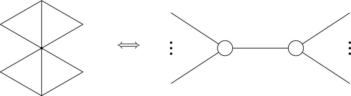
We now translate this reconstruction strategy into the polygon language used throughout the rest of the section. In this language, the three-point coefficient is represented by a triangle, which serves as the elementary building block for higher-point polygons: \[\tag{65} \psi_3 \quad \longleftrightarrow \quad \begin{figure}\includegraphics[width=0.8\textwidth]{_pdflatex/jfpacisb.png}\tag{66}\end{figure} \quad \longleftrightarrow \quad \begin{figure}\includegraphics[width=0.8\textwidth]{_pdflatex/dcsvwfba.png}\tag{67}\end{figure}\]
For Yang–Mills, the three-point wavefunction coefficient takes the form \[\label{eq:three-point-wavefunction} \psi_3(\boldsymbol{\epsilon}_1,\boldsymbol{\epsilon}_2,\boldsymbol{\epsilon}_3;\boldsymbol{k}_1,\boldsymbol{k}_2,\boldsymbol{k}_3;k_1,k_2,k_3) = V_{123}\,C_3(k_1,k_2,k_3).\tag{68}\] The explicit expression for the three-point Yang–Mills block, \(\psi_3^{\mathrm{YM}}=V_{123}\,C_3(k_1,k_2,k_3)\), was given in 25 . The triangle in Eq. 65 should be read as the dual graph of the purely wavy cubic Feynman diagram shown on the right-hand side: each side of the triangle is dual to one external wavy leg.
The reconstruction problem can now be phrased recursively. Suppose that all lower-point wavefunction blocks have already been determined. For each planar chord configuration of the \(n\)-gon, as in Fig. 3, we first compute the corresponding discontinuity by cutting the internal chords and gluing the lower-point blocks with the spectral measure \[\prod_{e\in \mathcal{E}} \frac{dp_e}{2\pi i}\, \frac{1}{x_e^2+p_e^2},\] together with a transverse polarization sum on every cut gluon line. This produces the part of the answer with the prescribed discontinuities in the channels \(x_e\). Equivalently, it fixes all terms that can be detected by iterated cuts.
The glued answer is not yet the full Yang–Mills wavefunction. The transverse projectors appearing in the gluing introduce apparent OPE poles \(1/x_e^2\) in the channel variables \(x_e\). These poles are the momentum-space imprint of the longitudinal part of the internal propagator. Since the currents on the two sides of the exchanged line must be conserved with respect to the internal momentum, this longitudinal piece cannot leave a residue in the complete answer. Thus, after constructing the known cut part, we expand it near each channel, \[x_e\to 0,\] isolate the singular coefficient of the corresponding OPE pole, and add a contact-type term with the same pole structure, often written below as a \(1/x_e^2\) OPE pole, whose singular part cancels it. This terminology refers to the OPE singularity in the channel variable \(x_e\), not to a physical energy discontinuity. In this sense the contact terms are obtained directly from the known glued part: they are fixed by the condition \[\label{eq:ope-residue-cancellation-bootstrap} \underset{x_e=0}{\operatorname{Res}}\, \psi_n^{\mathrm{YM}}=0 \qquad \text{for every internal channel }e .\tag{69}\] For overlapping channels the same prescription is applied to simultaneous residues, which is why the five- and six-point contact sectors contain double- and triple-OPE pole terms.
Accordingly, we write schematically5 \[\label{eq:ym-bootstrap-split} \psi_n^{\mathrm{YM}} = \psi_{n,\mathrm{cut}}^{\mathrm{YM}} + \psi_{n,\mathrm{OPE}}^{\mathrm{YM}},\tag{70}\] where \(\psi_{n,\mathrm{cut}}^{\mathrm{YM}}\) is the sum over all glued chord configurations and \(\psi_{n,\mathrm{OPE}}^{\mathrm{YM}}\) is a rational completion invisible to those cuts. The pole part of \(\psi_{n,\mathrm{OPE}}^{\mathrm{YM}}\) is fixed by 69 , while any remaining purely local ambiguity is fixed by the correct flat-space total-energy pole.
The low-point examples below follow the same pattern: \[\begin{array}{c|c|c|c} \text{multiplicity} & \text{cut-detectable data} & \text{OPE completion} & \text{remaining local input} \\ \hline 4 & \text{two exchange channels} & b_s,b_t & \text{quartic contact }c\\ 5 & \text{two-chord and one-chord pentagons} & B_5 & \text{-}\\ 6 & \text{maximal and lower-codimension cuts} & B_6^{(3)},B_6^{(2)} & \text{-} \end{array}\] Together, the OPE completion and any remaining local input form the cut-invisible completion. This table is only a roadmap: the explicit formulas below show how the singular OPE coefficients are extracted and canceled in each case.
This reconstruction procedure is a reorganization of the momentum-space Feynman rules collected in Appendix 5. The part detected by cuts corresponds to transverse bulk-to-bulk propagation, represented below by wavy internal lines. The remaining no-cut part is built from the purely longitudinal sector and from the elementary quartic Yang–Mills contact vertex, as will be made explicit in the low-point examples.
3.3 Four-point reconstruction↩︎
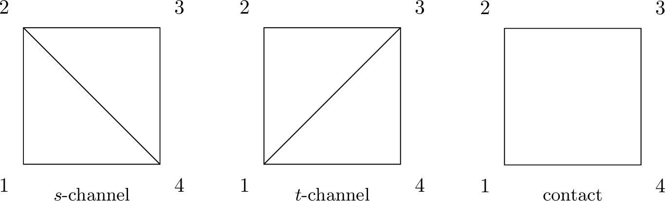
Four points are the first place where the distinction between the part generated by gluing and the cut-invisible completion becomes visible. In polygon language the answer receives three contributions, shown in Fig. 4: the two planar exchange channels and a zero-chord contact term. The exchange channels are reconstructed directly from their discontinuities, while the remaining contact contribution is fixed by current conservation and the flat-space limit.
\[\tag{71} \begin{align} \begin{figure}\includegraphics[width=0.8\textwidth]{_pdflatex/rtbdjise.png}\tag{72}\end{figure} &= \,-i\int_0^\infty \frac{dp_{13}}{2\pi i\,(x_{13}^2+p_{13}^2)} \sum_h \operatorname{Disc}_{p_{13}}\psi_3(\boldsymbol{\epsilon}_1,\boldsymbol{\epsilon}_2,\boldsymbol{\epsilon}_I^{(h)};\boldsymbol{k}_1,\boldsymbol{k}_2,-\boldsymbol{k}_1-\boldsymbol{k}_2;k_1,k_2,ip_{13}) \\ &\qquad\qquad\times \operatorname{Disc}_{p_{13}}\psi_3(\boldsymbol{\epsilon}_I^{(-h)},\boldsymbol{\epsilon}_3,\boldsymbol{\epsilon}_4;\boldsymbol{k}_1+\boldsymbol{k}_2,\boldsymbol{k}_3,\boldsymbol{k}_4;ip_{13},k_3,k_4) \\ &= \,-i\int_0^\infty \frac{dp_{13}}{2\pi i}\, \frac{ V_{12\mu}\,\Pi_{\boldsymbol{k}_{12}}^{\mu\nu}\,V_{\nu34}}{x_{13}^2+p_{13}^2}\, \bar C(k_1,k_2,i p_{13})\bar C(i p_{13},k_3,k_4) \\ &= V_{12\mu}\,\Pi_{\boldsymbol{k}_{12}}^{\mu\nu}\,V_{\nu34}\, \psi^{\mathrm{tr}\,\phi^3}_{4,13} \end{align}\] Here \(\psi^{\mathrm{tr}\,\phi^3}_{4,13}\) is the scalar four-point \(x_{13}\)-channel block evaluated in Eq. 51 .
This four-point example displays the basic reconstruction mechanism. The cut integral factorizes into a scalar discontinuity block and a tensor numerator obtained by gluing lower-point Yang–Mills vertices across the internal channel. The helicity sum on the cut line produces the transverse projector, \(\sum_h \boldsymbol{\epsilon}_I^{(h)\mu}\boldsymbol{\epsilon}_I^{(-h)\nu}=\Pi^{\mu\nu}\), so each planar chord contributes a local numerator dressing together with a purely spectral scalar factor.
The exchange contributions reconstructed from the discontinuity are not yet the complete four-point Yang–Mills wavefunction. In the \(s\)-channel, associated with \(x_{13}\) (equivalently \(x_{24}\)), current conservation requires the residue of the \(x_{13}^2\) pole to vanish. This pole is introduced by the transverse projector \(\Pi_{\boldsymbol{k}_{12}}^{\mu\nu}\) when we reconstruct the four-point exchange from two three-point building blocks. Its cancellation requires the additional terms \(b_s\) and \(b_t\), given in Eq. 73 . \[\label{eq:four-point-b} \begin{align} b_s &= -\frac{(\boldsymbol{\epsilon}_1\!\cdot\!\boldsymbol{\epsilon}_2)(\boldsymbol{\epsilon}_3\!\cdot\!\boldsymbol{\epsilon}_4) (k_1-k_2)(k_3-k_4)}{4\,x_{13}^2\,(k_1+k_2+k_3+k_4)}, \\ b_t &= \left.b_s\right|_{2\leftrightarrow4} = \frac{(\boldsymbol{\epsilon}_1\!\cdot\!\boldsymbol{\epsilon}_4)(\boldsymbol{\epsilon}_2\!\cdot\!\boldsymbol{\epsilon}_3) (k_1-k_4)(k_2-k_3)}{4\,x_{24}^2\,(k_1+k_2+k_3+k_4)}. \end{align}\tag{73}\] A contact contribution \(c\), given in Eq. 74 , is fixed by the flat-space limit. \[\label{eq:four-point-c} \begin{align} c &= \frac{V_4^{1234}}{E_4} = \frac{1}{2(k_1+k_2+k_3+k_4)} \bigl[ (\boldsymbol{\epsilon}_1\!\cdot\!\boldsymbol{\epsilon}_3)(\boldsymbol{\epsilon}_2\!\cdot\!\boldsymbol{\epsilon}_4) - \frac{1}{2}(\boldsymbol{\epsilon}_1\!\cdot\!\boldsymbol{\epsilon}_2)(\boldsymbol{\epsilon}_3\!\cdot\!\boldsymbol{\epsilon}_4) - \frac{1}{2}(\boldsymbol{\epsilon}_1\!\cdot\!\boldsymbol{\epsilon}_4)(\boldsymbol{\epsilon}_2\!\cdot\!\boldsymbol{\epsilon}_3) \bigr]. \end{align}\tag{74}\] Together, these terms assemble into the full zero-chord contribution
\[\tag{75} \begin{align} &B_4\!\left( \begin{array}{c} \boldsymbol{\epsilon}_1,\boldsymbol{\epsilon}_2,\boldsymbol{\epsilon}_3,\boldsymbol{\epsilon}_4\\ k_1,k_2,k_3,k_4\\ x_{13},x_{24} \end{array} \right) = \vcenter{\begin{figure}\includegraphics[width=0.8\textwidth]{_pdflatex/mngufapy.png}\tag{76}\end{figure}} = b_s+b_t+c \end{align}\]
Combining the two exchange reconstructions with the contact polygon, the four-point Yang–Mills wavefunction is written in polygon language as \[\tag{77} \psi_4^{\mathrm{YM}} = \begin{figure}\includegraphics[width=0.8\textwidth]{_pdflatex/retkyxfa.png}\tag{78}\end{figure} + \begin{figure}\includegraphics[width=0.8\textwidth]{_pdflatex/pncvagfs.png}\tag{79}\end{figure} + \begin{figure}\includegraphics[width=0.8\textwidth]{_pdflatex/iyqbgfjl.png}\tag{80}\end{figure}.\]
For the color ordering \((1,2,3,4)\), there is no independent planar \(u\)-channel triangulation of the quadrilateral. Comparing Eqs. 71 –74 with the explicit Feynman-rule computation summarized in Appendix 5, Eq. 119 , we find exact agreement: the two exchange polygons reproduce the transverse exchange diagrams, while the zero-chord quadrilateral, through the mixed-vertex rule and the shared dashed propagator in Eqs. 112 and 109 , reproduces the longitudinal exchanges. In addition, there is also a four-point contact diagram. The resulting four-point answer satisfies the conformal Ward identities and the expected soft behavior.
3.4 Five-point reconstruction↩︎
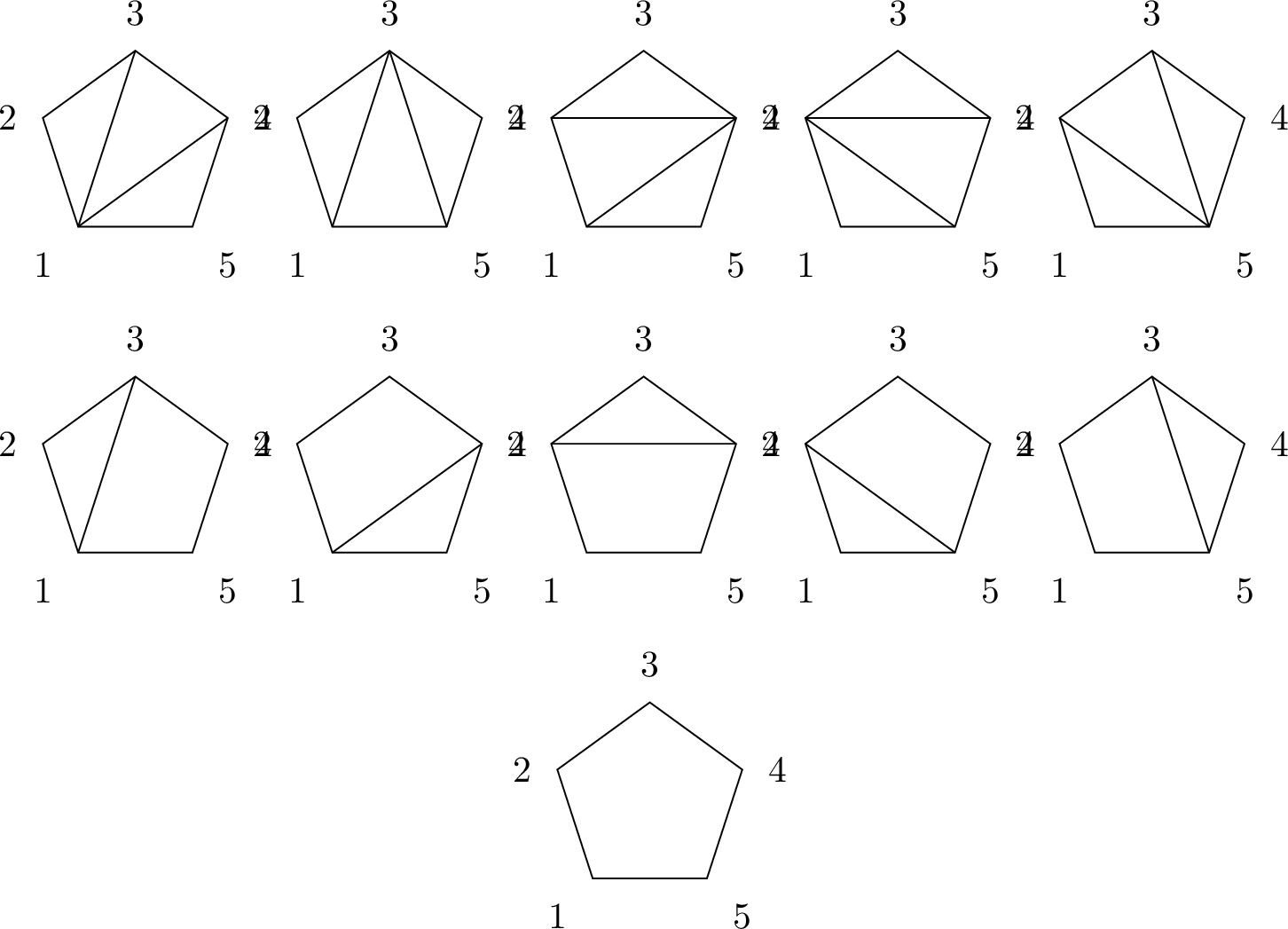
At five points the reconstruction problem becomes richer. Besides the fully triangulated polygons reconstructed from maximal cuts, one must also include one-chord and zero-chord sectors, and the role of current conservation is correspondingly more intricate. In polygon language, the answer is organized by the pentagon together with all its planar chord configurations.
For the color ordering \((1,2,3,4,5)\), we place the boundary labels clockwise starting from the lower-left vertex. The relevant configurations are displayed below.
We begin with a representative two-chord contribution, using \(\boldsymbol{k}_{12}:=\boldsymbol{k}_1+\boldsymbol{k}_2\) and \(\boldsymbol{k}_{123}:=\boldsymbol{k}_1+\boldsymbol{k}_2+\boldsymbol{k}_3\): \[\tag{81} \begin{align} \begin{figure}\includegraphics[width=0.8\textwidth]{_pdflatex/yotvfqbe.png}\tag{82}\end{figure} &= -\int_0^\infty \frac{dp_{13}}{2\pi i} \int_0^\infty \frac{dp_{14}}{2\pi i}\, \frac{ V_{12\mu}\,\Pi_{\boldsymbol{k}_{12}}^{\mu\nu}\,V_{\nu3\rho}\,\Pi_{\boldsymbol{k}_{123}}^{\rho\sigma}\,V_{\sigma45} }{(x_{13}^2+p_{13}^2)(x_{14}^2+p_{14}^2)} \\ &\qquad\times \bar C(k_1,k_2,i p_{13})\, \bar C(i p_{13},k_3,i p_{14})\, \bar C(i p_{14},k_4,k_5). \\ &= V_{12\mu}\,\Pi_{\boldsymbol{k}_{12}}^{\mu\nu}\,V_{\nu3\rho}\,\Pi_{\boldsymbol{k}_{123}}^{\rho\sigma}\,V_{\sigma45}\, \psi^{\mathrm{tr}\,\phi^3}_{5,13,14}. \end{align}\] As at four points, the result factorizes into a tensor numerator and the stripped scalar wavefunction \(\psi^{\mathrm{tr}\,\phi^3}_{5,13,14}\), given in 55 .
Next consider a representative one-chord contribution. With \(\boldsymbol{k}_{12}:=\boldsymbol{k}_1+\boldsymbol{k}_2\), \[\tag{83} \begin{align} \begin{figure}\includegraphics[width=0.8\textwidth]{_pdflatex/qcpnejsl.png}\tag{84}\end{figure} \\[-0.3em]&= -i\int_0^\infty \frac{dp_{13}}{2\pi i\,(x_{13}^2+p_{13}^2)} \sum_h \operatorname{Disc}_{p_{13}}\psi_3\!\left( \begin{array}{c} \boldsymbol{\epsilon}_1,\boldsymbol{\epsilon}_2,\boldsymbol{\epsilon}_I^{(h)}\\ \boldsymbol{k}_1,\boldsymbol{k}_2,-\boldsymbol{k}_{12}\\ k_1,k_2,ip_{13} \end{array} \right) \operatorname{Disc}_{p_{13}}B_4\!\left( \begin{array}{c} \boldsymbol{\epsilon}_I^{(-h)},\boldsymbol{\epsilon}_3,\boldsymbol{\epsilon}_4,\boldsymbol{\epsilon}_5\\ ip_{13},k_3,k_4,k_5\\ x_{14},x_{35} \end{array} \right). \\ &= \left(V_{12\mu}\,\Pi_{\boldsymbol{k}_{12}}^{\mu\nu}\,\boldsymbol{\epsilon}_{3\nu}\right) (\boldsymbol{\epsilon}_{4}\!\cdot\!\boldsymbol{\epsilon}_{5}) \left[\frac{(k_4-k_5)(2k_3+k_4+k_5)}{4\,\boldsymbol{k}_{45}^2}\right] \psi_{5,\,12|345}^{\mathrm{scalar}}+\,(3\leftrightarrow 5) \\ &\quad+ V_{12\mu}\,\Pi_{\boldsymbol{k}_{12}}^{\mu\nu}\,V_{\nu345}\, \psi_{5,\,12|345}^{\mathrm{scalar}}\end{align}\] Here \(\psi_{5,\,12|345}^{\mathrm{scalar}}\) denotes the scalar one-chord factor given explicitly in 121 . The first line is the longitudinal contribution from the quadrilateral, together with the reflected channel obtained by \(3\leftrightarrow 5\). The one-chord sector exhibits the first structural feature absent at four points: once a three-point block is glued to a lower-point contact block, the result is no longer captured by a single purely transverse tensor structure. It instead splits into a transverse piece and a pair of mixed corrections related by reflection.
By cyclically summing the double-chord contribution in 81 and the single-chord contribution in 83 , we obtain the part of the five-point answer generated purely by gluing lower-point polygon blocks: \[\tag{85} \begin{align} \psi_{5,\mathrm{cut}}^{\mathrm{YM}} &= \begin{figure}\includegraphics[width=0.8\textwidth]{_pdflatex/arzloeds.png}\tag{86}\end{figure} + \begin{figure}\includegraphics[width=0.8\textwidth]{_pdflatex/rkhgcsqa.png}\tag{87}\end{figure} +\mathrm{cyclic}. \end{align}\] This gluing-generated sum is the cut-detectable five-point part, but it is not yet the full answer. Some single-OPE residues remain, so current conservation is not yet manifest. The missing completion therefore belongs to the zero-chord sector. Equivalently, the cut-detectable part can be summarized as \[\label{eq:five-point-cut-bookkeeping} \psi_{5,\mathrm{cut}}^{\mathrm{YM}} = \sum_{\mathrm{cyc}} \left( \psi_{5}^{(2\mathrm{chord})} +\psi_{5}^{(1\mathrm{chord})} \right),\tag{88}\] where representative two-chord and one-chord terms are given in 81 and 83 .
3.4.0.1 Zero-chord completion.
To impose current conservation at five points, we require the residue of every single-OPE pole associated with an internal chord to vanish. For the pentagon these channels are \(x_{13}\), \(x_{14}\), \(x_{24}\), \(x_{25}\), and \(x_{35}\); equivalently, the coefficient of each corresponding \(1/x_{ij}^2\) pole must cancel in the full sum over polygon contributions. In practice, the zero-chord sector can be fixed by isolating the simultaneous residue of two single-OPE poles. For example, cancellation of the \(x_{13}^{-2}x_{14}^{-2}\) double pole fixes \[\label{eq:five-point-b5} \begin{align} B_5\!\left( \begin{array}{c} \boldsymbol{\epsilon}_1,\boldsymbol{\epsilon}_2,\boldsymbol{\epsilon}_3,\boldsymbol{\epsilon}_4,\boldsymbol{\epsilon}_5\\ \boldsymbol{k}_1,\boldsymbol{k}_2,\boldsymbol{k}_3,\boldsymbol{k}_4,\boldsymbol{k}_5\\ k_1,k_2,k_3,k_4,k_5\\ x_{13},x_{14} \end{array} \right) &= -\frac{ (k_1-k_2)(k_4-k_5) (\boldsymbol{\epsilon}_1\!\cdot\!\boldsymbol{\epsilon}_2) \bigl[\boldsymbol{\epsilon}_3\!\cdot\!(\boldsymbol{k}_4+\boldsymbol{k}_5)\bigr] (\boldsymbol{\epsilon}_4\!\cdot\!\boldsymbol{\epsilon}_5) }{ 4\,(k_1+k_2+k_3+k_4+k_5)\,x_{13}^2x_{14}^2 } \;+\;\mathrm{cyclic}. \end{align}\tag{89}\] The representative zero-chord polygon is therefore \[\tag{90} \begin{figure}\includegraphics[width=0.8\textwidth]{_pdflatex/sfjrondm.png}\tag{91}\end{figure} = B_5\!\left( \begin{array}{c} \boldsymbol{\epsilon}_1,\boldsymbol{\epsilon}_2,\boldsymbol{\epsilon}_3,\boldsymbol{\epsilon}_4,\boldsymbol{\epsilon}_5\\ \boldsymbol{k}_1,\boldsymbol{k}_2,\boldsymbol{k}_3,\boldsymbol{k}_4,\boldsymbol{k}_5\\ k_1,k_2,k_3,k_4,k_5\\ x_{13},x_{14} \end{array} \right).\] After adding this cyclic zero-chord contribution, the single-OPE singular parts cancel in the full cyclic sum. This is the five-point implementation of the current-conservation condition 69 .
Thus the full five-point Yang–Mills wavefunction takes the polygon form \[\tag{92}
\begin{align}
\psi_5^{\mathrm{YM}}
&=
\left(
\begin{figure}\includegraphics[width=0.8\textwidth]{_pdflatex/rnsecqtk.png}\tag{93}\end{figure}
+
\begin{figure}\includegraphics[width=0.8\textwidth]{_pdflatex/wciystkg.png}\tag{94}\end{figure}
+\mathrm{cyclic}
\right)
+
\begin{figure}\includegraphics[width=0.8\textwidth]{_pdflatex/purayoek.png}\tag{95}\end{figure}.
\end{align}\] Equivalently,
\[\label{eq:five-point-full-bookkeeping}
\psi_5^{\mathrm{YM}}
=
\sum_{\mathrm{cyc}}
\left(
\psi_{5}^{(2\mathrm{chord})}
+\psi_{5}^{(1\mathrm{chord})}
\right)
+B_5 .\tag{96}\] The full data are provided in the ancillary file 5ptYM and 6pt YM data.zip. The final five-point Yang–Mills wavefunction satisfies the expected \((A)dS\) soft theorem and
reproduces the correct flat-space limit. Comparing Eqs. 81 –89 with the explicit Feynman-rule organization in Appendix 5, Eqs. 122 –124 , we find that the reconstruction matches the direct Feynman-diagram computation: the maximally cut and one-chord polygon sectors reproduce the transverse and mixed
exchange topologies, while the remaining zero-chord pentagon supplies the contact and longitudinal completion. The one-chord contribution in Eq. 83 contains the factor \((k_4-k_5)(2k_3+k_4+k_5)\), which has a natural Feynman-diagrammatic interpretation in terms of the local propagator operations reviewed in Appendix 5.1.
3.5 Six-point reconstruction↩︎
At six points the space of chord configurations is large enough that it is most efficient to organize the reconstruction by topology. We begin with the ray-like maximal cuts, then turn to the non-ray-like maximal cuts, followed by the lower-codimension chord sectors, and finally determine the zero-chord part by cancelling the remaining higher-order OPE poles. Since the number of individual building blocks grows quickly at this multiplicity, we emphasize below the representative topologies and the logic by which they combine; more exhaustive diagrammatic summaries are collected in the appendix.
The representatives used below are:
| sector | representatives | orbit sizes | building blocks | ||
|---|---|---|---|---|---|
| maximal cuts |
|
\(6,3,3,2\) | \(\psi_3^4\) | ||
| two-chord sectors |
|
\(3,3,6,3\) | \(\psi_3 B_4\psi_3\) or \(\psi_3^2B_4\) | ||
| one-chord sectors | \((14),(13)\) | \(3,6\) | \(B_4B_4\) or \(\psi_3B_5\) | ||
| zero-chord sector | \(B_6^{(3)},B_6^{(2)}\) | \(6+3+3,\;6+3\) | OPE subtractions |
Here \((13|14|15)\) denotes the set of chords in the representative polygon, and the orbit size counts the number of distinct cyclic or reflected images included in the corresponding sum.
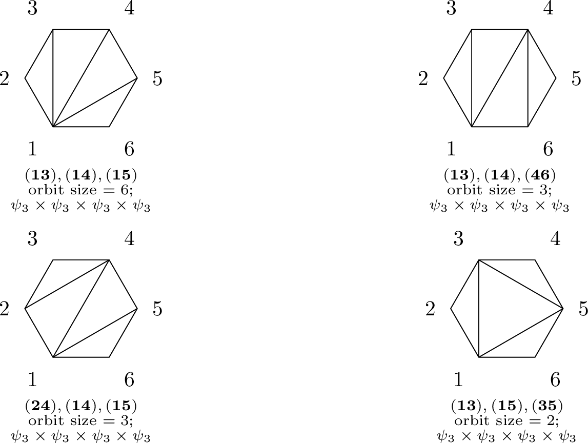
A representative gluing expression is \[\label{eq:six-point-raylike-131415-gluing} \begin{align} \psi_{6,\,13|14|15}^{\mathrm{YM}}(1,2,3,4,5,6) &= i\int_0^\infty \frac{dp_{13}}{2\pi i} \frac{dp_{14}}{2\pi i} \frac{dp_{15}}{2\pi i}\, \frac{ V_{12i}\, \Pi_{\boldsymbol{k}_{12}}^{ij}\, V_{j3l}\, \Pi_{\boldsymbol{k}_{123}}^{lm}\, V_{m4n}\, \Pi_{\boldsymbol{k}_{56}}^{nr}\, V_{r56} }{ (x_{13}^2+p_{13}^2) (x_{14}^2+p_{14}^2) (x_{15}^2+p_{15}^2) } \\ &\quad\times \bar C(k_1,k_2,ip_{13})\, \bar C(ip_{13},k_3,ip_{14})\, \bar C(ip_{14},k_4,ip_{15})\, \bar C(ip_{15},k_5,k_6),\\ &= \Bigl( V_{12i}\,\Pi_{\boldsymbol{k}_{12}}^{ij}\, V_{j3l}\,\Pi_{\boldsymbol{k}_{123}}^{lm}\, V_{m4n}\,\Pi_{\boldsymbol{k}_{56}}^{nr}\, V_{r56} \Bigr)\psi^{\mathrm{tr}\,\phi^3}_{6,13,14,15}. \end{align}\tag{97}\]
For a permutation \(i j k l m n\) of \(123456\), define \[\label{eq:six-point-rho-permutation} \rho_{i j k l m n}:\quad 123456\longmapsto i j k l m n .\tag{98}\] This relabelling acts on all labels, momenta, polarizations, and channels in the expression on its right. The two remaining maximally cut ray-like representatives are then generated from 97 by \[\begin{align} \psi_{6,\,13|14|46}^{\mathrm{YM}} &= \rho_{123654}\,\psi_{6,\,13|14|15}^{\mathrm{YM}}, \tag{99}\\ \psi_{6,\,24|14|15}^{\mathrm{YM}} &= \rho_{321456}\,\psi_{6,\,13|14|15}^{\mathrm{YM}}. \tag{100} \end{align}\]
\[\label{eq:six-point-131535-gluing} \begin{align} \psi_{6,\,13|15|35}^{\mathrm{YM}}(1,2,3,4,5,6) &= i\int_0^\infty \frac{dp_{13}}{2\pi i} \frac{dp_{15}}{2\pi i} \frac{dp_{35}}{2\pi i}\, \frac{ V_{12i}\, \Pi_{\boldsymbol{k}_{12}}^{ij}\, V_{jln}\, \Pi_{\boldsymbol{k}_{34}}^{lm}\, V_{m34}\, \Pi_{\boldsymbol{k}_{56}}^{nr}\, V_{r56} }{ (x_{13}^2+p_{13}^2) (x_{15}^2+p_{15}^2) (x_{35}^2+p_{35}^2) } \\ &\quad\times \bar C(k_1,k_2,ip_{13})\, \bar C(ip_{13},ip_{35},ip_{15})\, \bar C(ip_{35},k_3,k_4)\, \bar C(ip_{15},k_5,k_6),\\ &= \Bigl( V_{12i}\,\Pi_{\boldsymbol{k}_{12}}^{ij}\, V_{jln}\,\Pi_{\boldsymbol{k}_{34}}^{lm}\, V_{m34}\,\Pi_{\boldsymbol{k}_{56}}^{nr}\, V_{r56} \Bigr) \psi_{6,\,12|34|56}^{\mathrm{scalar}}. \end{align}\tag{101}\] Together, 97 – 101 provide one representative for each maximal six-point topology class; the remaining maximal cuts are generated by cyclic images in 108 .
3.5.0.1 Two-chord sectors.

\[\label{eq:six-point-1346-gluing} \begin{align} \psi_{6,\,13|46}^{\mathrm{YM}}(1,2,3,4,5,6) &= -\int_0^\infty \frac{dp_{13}}{2\pi i} \frac{dp_{46}}{2\pi i}\, \frac{ V_{12i}\, \Pi_{\boldsymbol{k}_{12}}^{ij}\, B_{4,j3l6}\, \Pi_{\boldsymbol{k}_{45}}^{lm}\, V_{m45} }{ (x_{13}^2+p_{13}^2) (x_{46}^2+p_{46}^2) } \\ &\quad\times \bar C(k_1,k_2,ip_{13})\, \bar C(ip_{46},k_4,k_5). \\ &= \psi_{6,\,12|36|45}^{(\mu\mu)} + \left( \rho_{123654} + \rho_{216345} \right) \psi_{6,\,12|3|4|56}^{(\mu z\mu)}. \end{align}\tag{102}\] where \[B_{4,j3l6} := \frac{\partial}{\partial \boldsymbol{\epsilon}_I^{j}} \frac{\partial}{\partial \boldsymbol{\epsilon}_J^{l}}\, \operatorname{Disc}_{p_{13}}\operatorname{Disc}_{p_{46}}\, B_4\!\left( \begin{array}{c} \boldsymbol{\epsilon}_I,\boldsymbol{\epsilon}_3,\boldsymbol{\epsilon}_J,\boldsymbol{\epsilon}_6\\ ip_{13},k_3,ip_{46},k_6\\ x_{14},x_{36} \end{array} \right).\]
The Feynman-rule blocks used in the last line, \(\psi_{6,\,12|36|45}^{(\mu\mu)}\) and \(\psi_{6,\,12|3|4|56}^{(\mu z\mu)}\), are given in 130 and the indicated relabellings of 143 .
\[\label{eq:six-point-1315-gluing} \begin{align} \psi_{6,\,13|15}^{\mathrm{YM}}(1,2,3,4,5,6) &= -\int_0^\infty \frac{dp_{13}}{2\pi i} \frac{dp_{15}}{2\pi i}\, \frac{ V_{12i}\, \Pi_{\boldsymbol{k}_{12}}^{ij}\, B_{4,j34l}\, \Pi_{\boldsymbol{k}_{56}}^{lm}\, V_{m56} }{ (x_{13}^2+p_{13}^2) (x_{15}^2+p_{15}^2) } \\ &\quad\times \bar C(k_1,k_2,ip_{13})\, \bar C(ip_{15},k_5,k_6). \\ &= \psi_{6,\,12|34|56}^{(\mu\mu)} + \psi_{6,\,12|3|4|56}^{(\mu z\mu)} + \rho_{345612}\, \psi_{6,\,12|34|56}^{(\mu\mu z)}. \end{align}\tag{103}\] where \[B_{4,j34l} := \frac{\partial}{\partial \boldsymbol{\epsilon}_I^{j}} \frac{\partial}{\partial \boldsymbol{\epsilon}_J^{l}}\, \operatorname{Disc}_{p_{13}}\operatorname{Disc}_{p_{15}}\, B_4\!\left( \begin{array}{c} \boldsymbol{\epsilon}_I,\boldsymbol{\epsilon}_3,\boldsymbol{\epsilon}_4,\boldsymbol{\epsilon}_J\\ ip_{13},k_3,k_4,ip_{15}\\ x_{14},x_{35} \end{array} \right).\]
The three terms in the last line, \(\psi_{6,\,12|34|56}^{(\mu\mu)}\), \(\psi_{6,\,12|3|4|56}^{(\mu z\mu)}\), and \(\psi_{6,\,12|34|56}^{(\mu\mu z)}\), are displayed in 129 , 143 , and 146 , respectively.
\[\label{eq:six-point-1314-gluing} \begin{align} \psi_{6,\,13|14}^{\mathrm{YM}}(1,2,3,4,5,6) &= -\int_0^\infty \frac{dp_{13}}{2\pi i} \frac{dp_{14}}{2\pi i}\, \frac{ V_{12i}\, \Pi_{\boldsymbol{k}_{12}}^{ij}\, V_{j3l}\, \Pi_{\boldsymbol{k}_{123}}^{lm}\, B_{4,m456} }{ (x_{13}^2+p_{13}^2) (x_{14}^2+p_{14}^2) } \\ &\quad\times \bar C(k_1,k_2,ip_{13})\, \bar C(ip_{13},k_3,ip_{14}). \\ &= \psi_{6,\,12|3|456}^{(\mu\mu)} \;+\; \left(1+\rho_{123654}\right) \psi_{6,\,12|3|4|56}^{(\mu\mu z)}. \end{align}\tag{104}\] The two block types in the last line, \(\psi_{6,\,12|3|456}^{(\mu\mu)}\) and \(\psi_{6,\,12|3|4|56}^{(\mu\mu z)}\), are given in 128 and 133 . The reflected partner is \[\label{eq:six-point-2414-gluing} \psi_{6,\,24|14}^{\mathrm{YM}} = \rho_{321456}\,\psi_{6,\,13|14}^{\mathrm{YM}}.\tag{105}\]
3.5.0.2 One-chord sectors.
\[\label{eq:six-point-14-gluing} \begin{align} \psi_{6,\,14}^{\mathrm{YM}}(1,2,3,4,5,6) &= -i\int_0^\infty \frac{dp_{14}}{2\pi i}\, \frac{ B_{4,123i}\, \Pi_{\boldsymbol{k}_{123}}^{ij}\, B_{4,j456} }{ x_{14}^2+p_{14}^2 }\\ &= \psi_{6,\,123|456}^{(\mu)} +\left( 1+\rho_{123654}+\rho_{321456}+\rho_{321654} \right) \psi_{6,\,12|3|4|56}^{(z\mu z)} \\ &\quad +\left( 1+\rho_{321456}+\rho_{654321} +\rho_{456321} \right) \psi_{6,\,12|3|456}^{(z\mu)}. \end{align}\tag{106}\] where \[\begin{align} B_{4,123i} &:= \frac{\partial}{\partial \boldsymbol{\epsilon}_I^{i}}\, \operatorname{Disc}_{p_{14}}\, B_4\!\left( \begin{array}{c} \boldsymbol{\epsilon}_1,\boldsymbol{\epsilon}_2,\boldsymbol{\epsilon}_3,\boldsymbol{\epsilon}_I\\ k_1,k_2,k_3,ip_{14}\\ x_{13},x_{24} \end{array} \right),\\ B_{4,j456} &:= \frac{\partial}{\partial \boldsymbol{\epsilon}_J^{j}}\, \operatorname{Disc}_{p_{14}}\, B_4\!\left( \begin{array}{c} \boldsymbol{\epsilon}_J,\boldsymbol{\epsilon}_4,\boldsymbol{\epsilon}_5,\boldsymbol{\epsilon}_6\\ ip_{14},k_4,k_5,k_6\\ x_{15},x_{46} \end{array} \right). \end{align}\]
The three block types in the last two lines, \(\psi_{6,\,123|456}^{(\mu)}\), \(\psi_{6,\,12|3|4|56}^{(z\mu z)}\), and \(\psi_{6,\,12|3|456}^{(z\mu)}\), are given in 131 , 137 , and 134 , with the displayed relabellings.
\[\begin{align} \psi_{6,\,13}^{\mathrm{YM}}(1,2,3,4,5,6) &= -i\int_0^\infty \frac{dp_{13}}{2\pi i}\, \frac{ V_{12i}\, \Pi_{\boldsymbol{k}_{12}}^{ij}\, B_{5,j3456} }{ x_{13}^2+p_{13}^2 } \bar C(k_1,k_2,ip_{13}).\\ &= \left( 1+\rho_{123654} +\rho_{216345} +\rho_{216543} \right) \psi_{6,\,12|3|4|56}^{(\mu zz)} +\psi_{6,\,12|34|56}^{(\mu zz)}. \end{align} \label{eq:six-point-13-gluing}\tag{107}\] where \[B_{5,j3456} := \frac{\partial}{\partial \boldsymbol{\epsilon}_I^{j}}\, \operatorname{Disc}_{p_{13}}\, B_5\!\left( \begin{array}{c} \boldsymbol{\epsilon}_I,\boldsymbol{\epsilon}_3,\boldsymbol{\epsilon}_4,\boldsymbol{\epsilon}_5,\boldsymbol{\epsilon}_6\\ \boldsymbol{k}_{12},\boldsymbol{k}_3,\boldsymbol{k}_4,\boldsymbol{k}_5,\boldsymbol{k}_6\\ ip_{13},k_3,k_4,k_5,k_6\\ x_{14},x_{15},x_{35},x_{36},x_{46} \end{array} \right).\]
The two block types in the last line, \(\psi_{6,\,12|3|4|56}^{(\mu zz)}\) and \(\psi_{6,\,12|34|56}^{(\mu zz)}\), are given in 136 and 138 , together with the displayed relabellings.
Let \[E_6:=k_1+k_2+k_3+k_4+k_5+k_6,\] and let \(\sigma\) denote the one-step cyclic relabelling \[\sigma:\quad i\mapsto i+1\quad (\mathrm{mod}\;6), \qquad x_{ij}\mapsto x_{i+1,j+1}.\] In the sums below, \(\sum_{\sigma\in\mathbb{Z}_m}\sigma[\cdots]\) means the sum over the \(m\) distinct cyclic images generated by this relabelling.
Summing the maximally cut and lower-codimension sectors constructed above, we obtain the cut-detectable six-point part \[\label{eq:six-point-minimal-cut-sum} \begin{align} \psi_{6,\mathrm{cut}}^{\mathrm{YM}} :={}& \sum_{\text{cut sectors}}\psi_{6,\text{sector}}^{\mathrm{YM}} \\ ={}& \sum_{\sigma\in\mathbb{Z}_6}\sigma\!\left[ \psi_{6,\,13|14|15}^{\mathrm{YM}}\right] + \sum_{\sigma\in\mathbb{Z}_3}\sigma\!\left[ \psi_{6,\,13|14|46}^{\mathrm{YM}}\right] + \sum_{\sigma\in\mathbb{Z}_3}\sigma\!\left[ \psi_{6,\,24|14|15}^{\mathrm{YM}}\right] + \sum_{\sigma\in\mathbb{Z}_2}\sigma\!\left[ \psi_{6,\,13|15|35}^{\mathrm{YM}}\right] \\ &+ \sum_{\sigma\in\mathbb{Z}_3}\sigma\!\left[ \psi_{6,\,13|46}^{\mathrm{YM}}\right] + \sum_{\sigma\in\mathbb{Z}_3}\sigma\!\left[ \psi_{6,\,24|14}^{\mathrm{YM}}\right] + \sum_{\sigma\in\mathbb{Z}_6}\sigma\!\left[ \psi_{6,\,13|15}^{\mathrm{YM}}\right] + \sum_{\sigma\in\mathbb{Z}_3}\sigma\!\left[ \psi_{6,\,13|14}^{\mathrm{YM}}\right] \\ &+ \sum_{\sigma\in\mathbb{Z}_3}\sigma\!\left[ \psi_{6,\,14}^{\mathrm{YM}}\right] + \sum_{\sigma\in\mathbb{Z}_6}\sigma\!\left[ \psi_{6,\,13}^{\mathrm{YM}}\right] . \end{align}\tag{108}\]
3.5.0.3 Zero-chord completion.
After summing the cut polygons, the remaining zero-chord six-point sector is determined by the requirement that the spurious higher-order OPE poles cancel in the full answer. In practice, this means subtracting the triple-OPE and double-OPE pieces that remain in the minimal-basis expression obtained from the cut contributions.
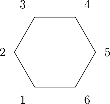
First, the triple-OPE sector is \[B_6^{(3)} = \sum_{\sigma\in\mathbb{Z}_6}\sigma\!\left[B_{6,\,13|14|15}^{(3)}\right] + \sum_{\sigma\in\mathbb{Z}_3}\sigma\!\left[B_{6,\,13|14|46}^{(3)}\right] + \sum_{\sigma\in\mathbb{Z}_3}\sigma\!\left[B_{6,\,13|36|46}^{(3)}\right],\] with representatives \[B_{6,\,13|14|15}^{(3)} = \frac{ (k_1-k_2)(k_5-k_6) (\boldsymbol{\epsilon}_1\!\cdot\!\boldsymbol{\epsilon}_2) \bigl[\boldsymbol{\epsilon}_3\!\cdot\!(\boldsymbol{k}_1+\boldsymbol{k}_2)\bigr] \bigl[\boldsymbol{\epsilon}_4\!\cdot\!(\boldsymbol{k}_1+\boldsymbol{k}_2+\boldsymbol{k}_3)\bigr] (\boldsymbol{\epsilon}_5\!\cdot\!\boldsymbol{\epsilon}_6) }{ 4E_6 x_{13}^2x_{14}^2x_{15}^2 },\] \[B_{6,\,13|14|46}^{(3)} = \frac{ (k_1-k_2)(k_4-k_5) (\boldsymbol{\epsilon}_1\!\cdot\!\boldsymbol{\epsilon}_2) \bigl[\boldsymbol{\epsilon}_3\!\cdot\!(\boldsymbol{k}_1+\boldsymbol{k}_2)\bigr] (\boldsymbol{\epsilon}_4\!\cdot\!\boldsymbol{\epsilon}_5) \bigl[\boldsymbol{\epsilon}_6\!\cdot\!(\boldsymbol{k}_4+\boldsymbol{k}_5)\bigr] }{ 4E_6 x_{13}^2x_{14}^2x_{46}^2 },\] and \[B_{6,\,13|36|46}^{(3)} = -\frac{ (k_1-k_2)(k_4-k_5) (\boldsymbol{\epsilon}_1\!\cdot\!\boldsymbol{\epsilon}_2) \bigl[\boldsymbol{\epsilon}_3\!\cdot\!(\boldsymbol{k}_4+\boldsymbol{k}_5)\bigr] (\boldsymbol{\epsilon}_4\!\cdot\!\boldsymbol{\epsilon}_5) \bigl[\boldsymbol{\epsilon}_6\!\cdot\!(\boldsymbol{k}_3+\boldsymbol{k}_4+\boldsymbol{k}_5)\bigr] }{ 4E_6 x_{13}^2x_{36}^2x_{46}^2 }.\]
Second, the double-OPE sector is \[B_6^{(2)} = \sum_{\sigma\in\mathbb{Z}_6}\sigma\!\left[B_{6,\,13|15}^{(2)}\right] + \sum_{\sigma\in\mathbb{Z}_3}\sigma\!\left[B_{6,\,13|46}^{(2)}\right],\] with representatives \[B_{6,\,13|15}^{(2)} = -\frac{ (k_1-k_2)(k_5-k_6) (\boldsymbol{\epsilon}_1\!\cdot\!\boldsymbol{\epsilon}_2) (\boldsymbol{\epsilon}_3\!\cdot\!\boldsymbol{\epsilon}_4) (\boldsymbol{\epsilon}_5\!\cdot\!\boldsymbol{\epsilon}_6) }{ 16E_6 x_{13}^2x_{15}^2 },\] and \[B_{6,\,13|46}^{(2)} = \frac{ (k_1-k_2)(k_4-k_5) (\boldsymbol{\epsilon}_1\!\cdot\!\boldsymbol{\epsilon}_2) (\boldsymbol{\epsilon}_3\!\cdot\!\boldsymbol{\epsilon}_6) (\boldsymbol{\epsilon}_4\!\cdot\!\boldsymbol{\epsilon}_5) }{ 8E_6 x_{13}^2x_{46}^2 }.\]
The zero-chord contact contribution is therefore \[\psi_{6,\mathrm{OPE}}^{\mathrm{YM}} = -B_6^{(3)} - B_6^{(2)}.\] This agrees with the Feynman-rule representative in Appendix 5: Eq. 135 gives the double-OPE contact subtractions, while Eq. 142 gives the triple-OPE completion.
Thus the full six-point Yang–Mills wavefunction is \[\psi_6^{\mathrm{YM}}
=
\psi_{6,\mathrm{cut}}^{\mathrm{YM}}
+
\psi_{6,\mathrm{OPE}}^{\mathrm{YM}}.\] The full data are provided in the ancillary file 5ptYM and 6pt YM data.zip. One can check that this full answer satisfies the single-OPE constraints: the OPE singular coefficient in every
single-channel limit vanishes after the cyclic sums in \(B_6^{(3)}\) and \(B_6^{(2)}\) are included, and the result also reproduces the expected soft behavior and correct flat-space
limit.
3.6 All-\(n\) structure suggested by low points↩︎
The low-point results suggest that the useful scalar reference theory is not pure \(\phi^3\), but the planar scalar theory with cubic and quartic vertices. At fixed cyclic ordering, the scalar sectors are dissections of an \(n\)-gon into triangles and quadrilaterals. For the first three nontrivial multiplicities this gives \[\begin{array}{c|c|c|c|c} n & \text{all cubic} & \text{one quartic vertex} & \text{two quartic vertices} & \text{total}\\ \hline 4 & 2 & 1 & 0 & 3\\ 5 & 5 & 5 & 0 & 10\\ 6 & 14 & 21 & 3 & 38 \end{array}\] Thus the no-dashed Yang–Mills terms follow the same counting as the color-ordered \(\phi^3+\phi^4\) scalar wavefunction. Each such scalar tubing carries the total-energy and partial-energy poles, while Yang–Mills supplies a local numerator built from cubic or quartic vertices and transverse projectors.
The longitudinal sector acts on a smaller subset of these scalar tubings. In a candidate replacement, one or more transverse internal propagators are replaced by dashed propagators. Most candidate replacements are absent or vanish, because the Yang–Mills three- and four-point vertices have special longitudinal contractions. When the replacement is nonzero and the dashed line touches an external rooted block, the effect is still simple: the dashed propagator collapses the original tubing to a more contact-like scalar wavefunction, and the numerator is reduced by the local collapse factors reviewed in Appendix 5.1. At five points this is already visible in the mixed \(3\ast3\ast3\) graphs, which reuse the scalar wavefunction of the \(3\ast4\) sector, and in the fully longitudinal graph, which is proportional to the contact scalar factor \(1/E_5\).
Six points make the same rule more explicit. The ordinary no-dashed sectors are the \(38\) planar \(\phi^3+\phi^4\) scalar tubings listed above. The nonzero dashed replacements include single- and double-dashed variants of the chain and star representatives. The terms in Eqs. 132 and 135 , for example, still have the expected form: a simplified Yang–Mills numerator multiplying an ordinary scalar tubing or a collapsed contact-type scalar tubing. Purely longitudinal chains, such as Eq. 139 , reduce further to zero-chord contact contributions.
The first correction to this proportionality appears when the dashed propagator is purely internal. In that case the local collapse is no longer simply a Yang–Mills numerator times the scalar wavefunction associated with the original tubing. The six-point examples in Eqs. 143 and 146 show this directly: the answer can still be written as a local operation on scalar tubings, but it contains an additional internal-collapse correction. This correction is not an arbitrary new pole structure. It is localized, tied to the dashed internal line, and constrained by current conservation and by the cancellation of spurious OPE singularities.
The resulting all-\(n\) pattern is therefore concrete. One starts with the planar \(\phi^3+\phi^4\) scalar tubings and dresses each no-dashed tubing by its Yang–Mills numerator. One then applies the allowed dashed-propagator replacements: many vanish, while the nonzero replacements either collapse to more contact-like scalar wavefunctions or, from six points onward, generate localized internal-collapse corrections when the dashed line is purely internal. Schematically, \[\psi_n^{\mathrm{YM}} = \sum_{\Gamma\in{\cal T}^{\phi^3+\phi^4}_n} N_\Gamma^{\mathrm{YM}}\, \psi_\Gamma^{\phi^3+\phi^4} + \sum_{\Gamma\in{\cal D}_n} \widetilde{N}_\Gamma^{\mathrm{YM}}\, \psi_{\mathrm{coll}(\Gamma)}^{\phi^3+\phi^4} + \Delta_n^{\mathrm{int}} .\] Here \({\cal T}^{\phi^3+\phi^4}_n\) denotes ordinary planar scalar tubings, \({\cal D}_n\) denotes the smaller set of nonzero dashed replacements, and \(\Delta_n^{\mathrm{int}}\) denotes the purely internal dashed-line corrections. The pole structure is therefore largely inherited from scalar wavefunctions. The remaining all-\(n\) problem is to organize the Yang–Mills numerators and the sparse internal-collapse corrections, perhaps through graph relations analogous to BCJ Jacobi identities or through a compact set of local moves on scalar tubings.
4 Conclusions and outlook↩︎
In this paper we studied tree-level Yang–Mills de Sitter wavefunction coefficients in momentum space from the viewpoint of discontinuities. Our main goal was to turn the general cutting formalism into an explicit reconstruction framework for spinning observables. Concretely, we formulated the gluing rule for gluon discontinuities, worked out representative maximal and non-maximal cuts, reconstructed the four-, five-, and six-point wavefunction coefficients, and compared the resulting expressions with direct momentum-space Feynman-rule computations. Along the way, the examples revealed an organizing principle that appears to persist beyond low multiplicity: a cut-detectable part controlled by lower-point gluing data together with a cut-invisible completion fixed by current conservation, spurious-pole cancellation, local longitudinal-sector corrections, and the flat-space limit. The explicit results through six points should therefore be viewed both as a concrete validation of the discontinuity method and as low-point data from which a more systematic all-\(n\) organization can be sought.
The low-point answers also point to a possible geometric interpretation. In our representation, many terms look like cosmological-polytope-type scalar objects dressed by Yang–Mills numerators. This suggests asking whether the dressed graphs can be combined into a single geometric or combinatorial object, rather than organized diagram by diagram. Such a structure would have to encode the gluing/completion split directly in momentum space, for example through its boundaries, canonical form, or stratification. Even a partial answer would clarify how far the scalar polytope picture extends once tensor numerators are included [37], [38], [40], [41].
One natural next step is to pass from wavefunctions to correlators. Recent work has developed several tools for this purpose, including dressing rules, dispersive reconstruction, physical cut bases, and correlator discontinuities [8]–[16], [59]–[64]. The explicit wavefunction data constructed here provide a momentum-space starting point for an analogous reconstruction of spinning correlators.
Gravity is another immediate target. The ingredients used here—factorized discontinuities, gluing of lower-point building blocks, and a cut-invisible completion sector—should have gravitational analogues, although the tensor algebra is more restrictive and the size of the completion is not yet clear. Existing results on spinning \((A)dS\) observables, on-shell bootstrap constructions for gluons and gravitons, and amplitude-inspired routes from \(AdS\) data to cosmological observables give several possible starting points [5], [17], [18], [22], [46], [47], [65]–[67]. A concrete question is whether any double-copy-like organization survives at the level of de Sitter wavefunctions.
There are also kinematical and representation-theoretic refinements to pursue. One is a spinor-helicity description of the results obtained here. Since low-point answers often simplify in that language, special helicity sectors, especially all-plus configurations, may admit a more compact reconstruction from discontinuity data. Another is the possible relation to Grassmannian- or on-shell-diagram-like structures. In flat-space amplitudes, such frameworks reorganize factorization data more efficiently than Feynman-diagram expansions; the open question is whether an analogue remains for cosmological observables in momentum space [68]–[71].
Finally, the relation to positive geometry remains open. Some aspects of the organization are more transparent in Mellin space than in momentum space, but the momentum-space formulas here make the gluing data and completion terms explicit enough to test proposed geometric descriptions directly [36]–[38], [41]. At present, the precise relation to scaffolding-type constructions in momentum space remains unclear and deserves a more focused future discussion [72], [73].
The main lesson is that discontinuity data for spinning de Sitter observables are not only consistency checks. They are explicit enough to reconstruct momentum-space wavefunctions and structured enough to expose patterns that are hard to see in a direct Feynman-diagram expansion.
We would like to thank Qu Cao for collaboration at an early stage of this project. S.H. and Y.M. are supported by the National Natural Science Foundation of China under Grant Nos. 12225510 and 12447101, and by the New Cornerstone Science Foundation. J.M. is supported by the European Union (ERC, UNIVERSE PLUS, 101118787). Views and opinions expressed, however, are those of the authors only and do not necessarily reflect those of the European Union or the European Research Council Executive Agency. Neither the European Union nor the granting authority can be held responsible for them.
5 Momentum-space Feynman rules for Yang–Mills theory↩︎
For convenience, we collect here the conventions and elementary momentum-space Feynman rules used throughout the main text. We work in the radial coordinate \(z\), with \(k=|\boldsymbol{k}|\) denoting the boundary energy associated with a spatial momentum \(\boldsymbol{k}\). The external bulk-to-boundary propagator is \[K^i(z)=\boldsymbol{\epsilon}^i e^{-zk},\] while the transverse bulk-to-bulk propagator is written in spectral form as \[G^\perp_{ij}(z_1,z_2;k_s) := \Pi_{ij}^{(k_s)} \int_{-\infty}^{\infty}\frac{dp}{\pi}\, \frac{\sin(pz_1)\sin(pz_2)}{(k_s^2+p^2)}, \qquad \Pi_{ij}^{(k_s)} = \delta_{ij} -\frac{k_s^i k_s^j}{k_s^2}.\] The longitudinal propagator is local in the radial coordinate: \[G^\parallel_{zz}(z_1,z_2;k_I) = \frac{\delta(z_1-z_2)}{k_I^2}. \label{eq:ym-longitudinal-propagator}\tag{109}\] Each bulk vertex is accompanied by an integration, \[\int_0^\infty dz .\]
5.0.0.1 Three-point vertices.
Latin indices denote spatial components, while a \(z\) index denotes the radial direction. With all momenta taken outgoing, the cubic vertices that enter our computations are \[\begin{align} V_{ij\ell}(\boldsymbol{k}_1,\boldsymbol{k}_2,\boldsymbol{k}_3) &= \frac{1}{2}\Bigl[ \delta_{ij}(\boldsymbol{k}_1^\ell-\boldsymbol{k}_2^\ell) +\delta_{j\ell}(\boldsymbol{k}_2^i-\boldsymbol{k}_3^i) +\delta_{\ell i}(\boldsymbol{k}_3^j-\boldsymbol{k}_1^j) \Bigr], \tag{110} \\ V_{ijz}&= -\frac{i}{2}\,\delta_{ij}\, \bigl(\partial_{z_i}-\partial_{z_j}\bigr), \tag{111} \\ V_{izz}(\boldsymbol{k}_2,\boldsymbol{k}_3) &= \frac{1}{2}\bigl(\boldsymbol{k}_2^i-\boldsymbol{k}_3^i\bigr). \end{align}\]
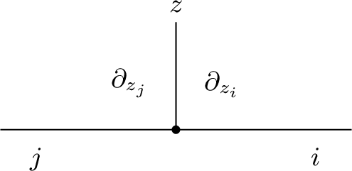
5.0.0.2 Four-point vertex.
The quartic Yang–Mills vertex is \[V_{\mu\nu\rho\sigma} = \frac{1}{2}\eta_{\mu\rho}\eta_{\nu\sigma} -\frac{1}{4}\bigl(\eta_{\mu\nu}\eta_{\rho\sigma}+\eta_{\mu\sigma}\eta_{\nu\rho}\bigr).\]
Here Greek indices run over both spatial and radial directions, \(\mu=i,z\), while Latin indices \(i,j,k,\ell,m,\ldots\) are spatial. The metric is the Minkowski metric, and we use \(\eta_{zz}=1\) and \(\eta_{ij}=\delta_{ij}\).
Since \(\eta_{zi}=0\), the only nonvanishing mixed \(z/i\) components of \(V_{\mu\nu\rho\sigma}\), apart from the purely spatial \(V_{ijkl}\), are \[V_{zzij}=V_{zijz}=V_{izzj}=V_{ijzz} = -\frac{1}{4}\eta_{zz}\eta_{ij}, \qquad V_{zizj}=V_{izjz} = \frac{1}{2}\eta_{zz}\eta_{ij}.\]
All remaining mixed components vanish; in particular, any component with an odd number of \(z\) indices is zero, and \(V_{zzzz}=0\).
The propagator factors above should be multiplied by the appropriate external waves and integrated over the radial coordinates of all vertices.
5.1 Special cases of internal longitudinal propagator↩︎
Mixed-vertex radial rule and collapse identity.
We now spell out the elementary identity responsible for the collapse terms appearing in the main text. In radial space the mixed cubic vertex with one radial index is represented by the differential operator \[\label{eq:vijz-radial-rule} V_{ijz} = -\frac{i}{2}\,\delta_{ij}\, \bigl(\partial_{z_i}-\partial_{z_j}\bigr).\tag{112}\] When both legs adjacent to the derivative are external, this operator acts on the two bulk-to-boundary propagators as \[\label{eq:vijz-on-external-btb} -\frac{i}{2} \bigl(\partial_{z_i}-\partial_{z_j}\bigr) \Bigl(e^{-k_i z}e^{-k_j z}\Bigr) = \frac{i}{2}(k_i-k_j)\,e^{-k_i z}e^{-k_j z},\tag{113}\] which reproduces the corresponding momentum-space mixed-vertex factor with \(q_i=k_i\) and \(q_j=k_j\).
The same derivative can instead hit an adjacent internal transverse line. For this purpose it is enough to use the scalar part of the spectral kernel, \[G(z_1,z_2;k_s) := \int_{-\infty}^{\infty}\frac{dp}{\pi}\, \frac{\sin(p z_1)\sin(p z_2)}{2i\,(k_s^2+p^2)}.\] Acting with the sum of derivatives at the two endpoints gives \[\label{eq:btb-derivative-sum} \begin{align} (\partial_{z_1}+\partial_{z_2})\,G(z_1,z_2;k_s) &= \int_{-\infty}^{\infty}\frac{dp}{\pi}\, \frac{ p\cos(p z_1)\sin(p z_2) + p\sin(p z_1)\cos(p z_2) }{2i\,(k_s^2+p^2)}\\ &= \int_{-\infty}^{\infty}\frac{dp}{\pi}\, \frac{p\,\sin\!\bigl(p(z_1+z_2)\bigr)}{2i\,(k_s^2+p^2)}\\ &= -\frac{i}{2} \int_{-\infty}^{\infty}\frac{dp}{\pi}\, \frac{p\,\sin\!\bigl(p(z_1+z_2)\bigr)}{k_s^2+p^2}. \end{align}\tag{114}\] For \(L>0\), the standard Fourier integral is \[\int_{-\infty}^{\infty}\frac{dp}{\pi}\, \frac{\cos(pL)}{k_s^2+p^2} = \frac{e^{-k_s L}}{k_s},\] and differentiating with respect to \(L\) gives \[\int_{-\infty}^{\infty}\frac{dp}{\pi}\, \frac{p\,\sin(pL)}{k_s^2+p^2} = e^{-k_s L}.\] Setting \(L=z_1+z_2\) in 114 , we therefore obtain \[\label{eq:btb-collapse-source} (\partial_{z_1}+\partial_{z_2})\,G(z_1,z_2;k_s) = -\frac{i}{2}\,e^{-k_s(z_1+z_2)}.\tag{115}\] Equivalently, the same propagator can be written as \[G(z_1,z_2;k_s) = -\frac{i}{4k_s} \Bigl( e^{-k_s|z_1-z_2|} - e^{-k_s(z_1+z_2)} \Bigr),\] so \((\partial_{z_1}+\partial_{z_2})\) annihilates the direct piece \(e^{-k_s|z_1-z_2|}\) and leaves only the image term \(e^{-k_s(z_1+z_2)}\). This surviving exponential is the propagator-collapse contribution packaged below into the operators \(\widehat{\mathcal{C}}_I\).
Figure 10: Schematic rooted-branch configuration for the local operator rule with two mixed vertices sharing a dashed propagator..
After the radial integration, it is useful to package a mixed cubic vertex \((V_{ijz})\) with one radial index as a local operator acting on a rooted scalar skeleton. For two rooted branches \(I,J\) meeting at such a vertex, as in Fig. 10, define \[\label{eq:local-operator-single} \widehat{\mathbb{V}}_{I,J} := \frac{1}{4} \Big[ (k_I-\widehat{\mathcal{C}}_I) - (k_J-\widehat{\mathcal{C}}_J) \Big],\tag{116}\] Here \(I,J\) stand for either the pair \(A,B\) or the pair \(C,D\) in Fig. 10, and \(k_I,k_J\) denote the sums of the energies carried by the outermost external legs of those rooted branches. The operators \(\widehat{\mathcal{C}}_I\) and \(\widehat{\mathcal{C}}_J\) are the propagator-collapse operators associated with the two rooted branches, namely the extra terms generated when one moves \(\partial_z\) outward so that it acts on the outermost external leg. Each time the derivative crosses an internal transverse propagator line, one picks up the corresponding product of bulk-to-boundary propagators. Let \(\psi_{0}^{\mathrm{cs}}\) denote the rooted scalar skeleton obtained after shrinking the dashed line.
For a pair of mixed vertices sharing the same dashed propagator \(1/q^2\), with four rooted branches \(A,B,C,D\), this becomes \[\label{eq:local-operator-double} \psi_{(A,B)\,||\,(C,D)}^{\mathrm{sc}} = \frac{1}{4\,q^2}\, \widehat{\mathbb{V}}_{A,B}\, \widehat{\mathbb{V}}_{C,D}\, \psi_{0}^{\mathrm{cs}}.\tag{117}\] Expanding the two operators gives \[\label{eq:local-operator-double-expanded} \begin{align} \psi_{(A,B)\,||\,(C,D)}^{\mathrm{sc}} &= \frac{1}{4\,q^2} \Big[ \bigl((k_A-k_B)-\widehat{\mathcal{C}}_A+\widehat{\mathcal{C}}_B\bigr) \bigl((k_C-k_D)-\widehat{\mathcal{C}}_C+\widehat{\mathcal{C}}_D\bigr) \Big] \psi_{0}^{\mathrm{cs}}\\ &= \frac{1}{4\,q^2} \Big[ (k_A-k_B)(k_C-k_D)\,\psi_{0}^{\mathrm{cs}} -(k_A-k_B)(\widehat{\mathcal{C}}_C-\widehat{\mathcal{C}}_D)\,\psi_{0}^{\mathrm{cs}}\\ & -(k_C-k_D)(\widehat{\mathcal{C}}_A-\widehat{\mathcal{C}}_B)\,\psi_{0}^{\mathrm{cs}} +(\widehat{\mathcal{C}}_A-\widehat{\mathcal{C}}_B) (\widehat{\mathcal{C}}_C-\widehat{\mathcal{C}}_D)\,\psi_{0}^{\mathrm{cs}} \Big]. \end{align}\tag{118}\] We have checked this relation against 143 .
Diagrammatically this reads:
\[{!}{ \begin{align} \psi_{(A,B)\,||\,(C,D)}^{\mathrm{sc}} = \frac{1}{16\,q^2}\Big[& (k_A-k_B)(k_C-k_D)\,\begin{tikzpicture}[baseline=-0.6ex,x=0.85cm,y=0.85cm,every node/.style={font=\scriptsize}] \coordinate (O) at (0,0); \coordinate (A) at (-1.35,-0.95); \coordinate (B) at (-1.35, 0.95); \coordinate (C) at ( 1.35, 0.95); \coordinate (D) at ( 1.35,-0.95); \draw[line width=0.85pt] (O) -- (A); \draw[line width=0.85pt] (O) -- (B); \draw[line width=0.85pt] (O) -- (C); \draw[line width=0.85pt] (O) -- (D); \fill (O) circle (1.5pt); \node[draw,circle,fill=white,fill opacity=1,text opacity=1,inner sep=1.0pt,minimum size=12pt] at (A) {A}; \node[draw,circle,fill=white,fill opacity=1,text opacity=1,inner sep=1.0pt,minimum size=12pt] at (B) {B}; \node[draw,circle,fill=white,fill opacity=1,text opacity=1,inner sep=1.0pt,minimum size=12pt] at (C) {C}; \node[draw,circle,fill=white,fill opacity=1,text opacity=1,inner sep=1.0pt,minimum size=12pt] at (D) {D}; \ifnum 0=1 \draw[line width=0.8pt] (-0.62,-0.18) -- (-0.32,-0.52); \fi \ifnum 0=1 \draw[line width=0.8pt] (-0.62,0.18) -- (-0.32,0.52); \fi \ifnum 0=1 \draw[line width=0.8pt] (0.32,0.52) -- (0.62,0.18); \fi \ifnum 0=1 \draw[line width=0.8pt] (0.32,-0.52) -- (0.62,-0.18); \fi \end{tikzpicture}\\[0.4em] &-(k_A-k_B)\Big( \begin{tikzpicture}[baseline=-0.6ex,x=0.85cm,y=0.85cm,every node/.style={font=\scriptsize}] \coordinate (O) at (0,0); \coordinate (A) at (-1.35,-0.95); \coordinate (B) at (-1.35, 0.95); \coordinate (C) at ( 1.35, 0.95); \coordinate (D) at ( 1.35,-0.95); \draw[line width=0.85pt] (O) -- (A); \draw[line width=0.85pt] (O) -- (B); \draw[line width=0.85pt] (O) -- (C); \draw[line width=0.85pt] (O) -- (D); \fill (O) circle (1.5pt); \node[draw,circle,fill=white,fill opacity=1,text opacity=1,inner sep=1.0pt,minimum size=12pt] at (A) {A}; \node[draw,circle,fill=white,fill opacity=1,text opacity=1,inner sep=1.0pt,minimum size=12pt] at (B) {B}; \node[draw,circle,fill=white,fill opacity=1,text opacity=1,inner sep=1.0pt,minimum size=12pt] at (C) {C}; \node[draw,circle,fill=white,fill opacity=1,text opacity=1,inner sep=1.0pt,minimum size=12pt] at (D) {D}; \ifnum 0=1 \draw[line width=0.8pt] (-0.62,-0.18) -- (-0.32,-0.52); \fi \ifnum 0=1 \draw[line width=0.8pt] (-0.62,0.18) -- (-0.32,0.52); \fi \ifnum 1=1 \draw[line width=0.8pt] (0.32,0.52) -- (0.62,0.18); \fi \ifnum 0=1 \draw[line width=0.8pt] (0.32,-0.52) -- (0.62,-0.18); \fi \end{tikzpicture} - \begin{tikzpicture}[baseline=-0.6ex,x=0.85cm,y=0.85cm,every node/.style={font=\scriptsize}] \coordinate (O) at (0,0); \coordinate (A) at (-1.35,-0.95); \coordinate (B) at (-1.35, 0.95); \coordinate (C) at ( 1.35, 0.95); \coordinate (D) at ( 1.35,-0.95); \draw[line width=0.85pt] (O) -- (A); \draw[line width=0.85pt] (O) -- (B); \draw[line width=0.85pt] (O) -- (C); \draw[line width=0.85pt] (O) -- (D); \fill (O) circle (1.5pt); \node[draw,circle,fill=white,fill opacity=1,text opacity=1,inner sep=1.0pt,minimum size=12pt] at (A) {A}; \node[draw,circle,fill=white,fill opacity=1,text opacity=1,inner sep=1.0pt,minimum size=12pt] at (B) {B}; \node[draw,circle,fill=white,fill opacity=1,text opacity=1,inner sep=1.0pt,minimum size=12pt] at (C) {C}; \node[draw,circle,fill=white,fill opacity=1,text opacity=1,inner sep=1.0pt,minimum size=12pt] at (D) {D}; \ifnum 0=1 \draw[line width=0.8pt] (-0.62,-0.18) -- (-0.32,-0.52); \fi \ifnum 0=1 \draw[line width=0.8pt] (-0.62,0.18) -- (-0.32,0.52); \fi \ifnum 0=1 \draw[line width=0.8pt] (0.32,0.52) -- (0.62,0.18); \fi \ifnum 1=1 \draw[line width=0.8pt] (0.32,-0.52) -- (0.62,-0.18); \fi \end{tikzpicture} \Big)\\[0.4em] &-(k_C-k_D)\Big( \begin{tikzpicture}[baseline=-0.6ex,x=0.85cm,y=0.85cm,every node/.style={font=\scriptsize}] \coordinate (O) at (0,0); \coordinate (A) at (-1.35,-0.95); \coordinate (B) at (-1.35, 0.95); \coordinate (C) at ( 1.35, 0.95); \coordinate (D) at ( 1.35,-0.95); \draw[line width=0.85pt] (O) -- (A); \draw[line width=0.85pt] (O) -- (B); \draw[line width=0.85pt] (O) -- (C); \draw[line width=0.85pt] (O) -- (D); \fill (O) circle (1.5pt); \node[draw,circle,fill=white,fill opacity=1,text opacity=1,inner sep=1.0pt,minimum size=12pt] at (A) {A}; \node[draw,circle,fill=white,fill opacity=1,text opacity=1,inner sep=1.0pt,minimum size=12pt] at (B) {B}; \node[draw,circle,fill=white,fill opacity=1,text opacity=1,inner sep=1.0pt,minimum size=12pt] at (C) {C}; \node[draw,circle,fill=white,fill opacity=1,text opacity=1,inner sep=1.0pt,minimum size=12pt] at (D) {D}; \ifnum 1=1 \draw[line width=0.8pt] (-0.62,-0.18) -- (-0.32,-0.52); \fi \ifnum 0=1 \draw[line width=0.8pt] (-0.62,0.18) -- (-0.32,0.52); \fi \ifnum 0=1 \draw[line width=0.8pt] (0.32,0.52) -- (0.62,0.18); \fi \ifnum 0=1 \draw[line width=0.8pt] (0.32,-0.52) -- (0.62,-0.18); \fi \end{tikzpicture} - \begin{tikzpicture}[baseline=-0.6ex,x=0.85cm,y=0.85cm,every node/.style={font=\scriptsize}] \coordinate (O) at (0,0); \coordinate (A) at (-1.35,-0.95); \coordinate (B) at (-1.35, 0.95); \coordinate (C) at ( 1.35, 0.95); \coordinate (D) at ( 1.35,-0.95); \draw[line width=0.85pt] (O) -- (A); \draw[line width=0.85pt] (O) -- (B); \draw[line width=0.85pt] (O) -- (C); \draw[line width=0.85pt] (O) -- (D); \fill (O) circle (1.5pt); \node[draw,circle,fill=white,fill opacity=1,text opacity=1,inner sep=1.0pt,minimum size=12pt] at (A) {A}; \node[draw,circle,fill=white,fill opacity=1,text opacity=1,inner sep=1.0pt,minimum size=12pt] at (B) {B}; \node[draw,circle,fill=white,fill opacity=1,text opacity=1,inner sep=1.0pt,minimum size=12pt] at (C) {C}; \node[draw,circle,fill=white,fill opacity=1,text opacity=1,inner sep=1.0pt,minimum size=12pt] at (D) {D}; \ifnum 0=1 \draw[line width=0.8pt] (-0.62,-0.18) -- (-0.32,-0.52); \fi \ifnum 1=1 \draw[line width=0.8pt] (-0.62,0.18) -- (-0.32,0.52); \fi \ifnum 0=1 \draw[line width=0.8pt] (0.32,0.52) -- (0.62,0.18); \fi \ifnum 0=1 \draw[line width=0.8pt] (0.32,-0.52) -- (0.62,-0.18); \fi \end{tikzpicture} \Big)\\[0.4em] &+\Big( \begin{tikzpicture}[baseline=-0.6ex,x=0.85cm,y=0.85cm,every node/.style={font=\scriptsize}] \coordinate (O) at (0,0); \coordinate (A) at (-1.35,-0.95); \coordinate (B) at (-1.35, 0.95); \coordinate (C) at ( 1.35, 0.95); \coordinate (D) at ( 1.35,-0.95); \draw[line width=0.85pt] (O) -- (A); \draw[line width=0.85pt] (O) -- (B); \draw[line width=0.85pt] (O) -- (C); \draw[line width=0.85pt] (O) -- (D); \fill (O) circle (1.5pt); \node[draw,circle,fill=white,fill opacity=1,text opacity=1,inner sep=1.0pt,minimum size=12pt] at (A) {A}; \node[draw,circle,fill=white,fill opacity=1,text opacity=1,inner sep=1.0pt,minimum size=12pt] at (B) {B}; \node[draw,circle,fill=white,fill opacity=1,text opacity=1,inner sep=1.0pt,minimum size=12pt] at (C) {C}; \node[draw,circle,fill=white,fill opacity=1,text opacity=1,inner sep=1.0pt,minimum size=12pt] at (D) {D}; \ifnum 1=1 \draw[line width=0.8pt] (-0.62,-0.18) -- (-0.32,-0.52); \fi \ifnum 0=1 \draw[line width=0.8pt] (-0.62,0.18) -- (-0.32,0.52); \fi \ifnum 1=1 \draw[line width=0.8pt] (0.32,0.52) -- (0.62,0.18); \fi \ifnum 0=1 \draw[line width=0.8pt] (0.32,-0.52) -- (0.62,-0.18); \fi \end{tikzpicture} - \begin{tikzpicture}[baseline=-0.6ex,x=0.85cm,y=0.85cm,every node/.style={font=\scriptsize}] \coordinate (O) at (0,0); \coordinate (A) at (-1.35,-0.95); \coordinate (B) at (-1.35, 0.95); \coordinate (C) at ( 1.35, 0.95); \coordinate (D) at ( 1.35,-0.95); \draw[line width=0.85pt] (O) -- (A); \draw[line width=0.85pt] (O) -- (B); \draw[line width=0.85pt] (O) -- (C); \draw[line width=0.85pt] (O) -- (D); \fill (O) circle (1.5pt); \node[draw,circle,fill=white,fill opacity=1,text opacity=1,inner sep=1.0pt,minimum size=12pt] at (A) {A}; \node[draw,circle,fill=white,fill opacity=1,text opacity=1,inner sep=1.0pt,minimum size=12pt] at (B) {B}; \node[draw,circle,fill=white,fill opacity=1,text opacity=1,inner sep=1.0pt,minimum size=12pt] at (C) {C}; \node[draw,circle,fill=white,fill opacity=1,text opacity=1,inner sep=1.0pt,minimum size=12pt] at (D) {D}; \ifnum 1=1 \draw[line width=0.8pt] (-0.62,-0.18) -- (-0.32,-0.52); \fi \ifnum 0=1 \draw[line width=0.8pt] (-0.62,0.18) -- (-0.32,0.52); \fi \ifnum 0=1 \draw[line width=0.8pt] (0.32,0.52) -- (0.62,0.18); \fi \ifnum 1=1 \draw[line width=0.8pt] (0.32,-0.52) -- (0.62,-0.18); \fi \end{tikzpicture} - \begin{tikzpicture}[baseline=-0.6ex,x=0.85cm,y=0.85cm,every node/.style={font=\scriptsize}] \coordinate (O) at (0,0); \coordinate (A) at (-1.35,-0.95); \coordinate (B) at (-1.35, 0.95); \coordinate (C) at ( 1.35, 0.95); \coordinate (D) at ( 1.35,-0.95); \draw[line width=0.85pt] (O) -- (A); \draw[line width=0.85pt] (O) -- (B); \draw[line width=0.85pt] (O) -- (C); \draw[line width=0.85pt] (O) -- (D); \fill (O) circle (1.5pt); \node[draw,circle,fill=white,fill opacity=1,text opacity=1,inner sep=1.0pt,minimum size=12pt] at (A) {A}; \node[draw,circle,fill=white,fill opacity=1,text opacity=1,inner sep=1.0pt,minimum size=12pt] at (B) {B}; \node[draw,circle,fill=white,fill opacity=1,text opacity=1,inner sep=1.0pt,minimum size=12pt] at (C) {C}; \node[draw,circle,fill=white,fill opacity=1,text opacity=1,inner sep=1.0pt,minimum size=12pt] at (D) {D}; \ifnum 0=1 \draw[line width=0.8pt] (-0.62,-0.18) -- (-0.32,-0.52); \fi \ifnum 1=1 \draw[line width=0.8pt] (-0.62,0.18) -- (-0.32,0.52); \fi \ifnum 1=1 \draw[line width=0.8pt] (0.32,0.52) -- (0.62,0.18); \fi \ifnum 0=1 \draw[line width=0.8pt] (0.32,-0.52) -- (0.62,-0.18); \fi \end{tikzpicture} + \begin{tikzpicture}[baseline=-0.6ex,x=0.85cm,y=0.85cm,every node/.style={font=\scriptsize}] \coordinate (O) at (0,0); \coordinate (A) at (-1.35,-0.95); \coordinate (B) at (-1.35, 0.95); \coordinate (C) at ( 1.35, 0.95); \coordinate (D) at ( 1.35,-0.95); \draw[line width=0.85pt] (O) -- (A); \draw[line width=0.85pt] (O) -- (B); \draw[line width=0.85pt] (O) -- (C); \draw[line width=0.85pt] (O) -- (D); \fill (O) circle (1.5pt); \node[draw,circle,fill=white,fill opacity=1,text opacity=1,inner sep=1.0pt,minimum size=12pt] at (A) {A}; \node[draw,circle,fill=white,fill opacity=1,text opacity=1,inner sep=1.0pt,minimum size=12pt] at (B) {B}; \node[draw,circle,fill=white,fill opacity=1,text opacity=1,inner sep=1.0pt,minimum size=12pt] at (C) {C}; \node[draw,circle,fill=white,fill opacity=1,text opacity=1,inner sep=1.0pt,minimum size=12pt] at (D) {D}; \ifnum 0=1 \draw[line width=0.8pt] (-0.62,-0.18) -- (-0.32,-0.52); \fi \ifnum 1=1 \draw[line width=0.8pt] (-0.62,0.18) -- (-0.32,0.52); \fi \ifnum 0=1 \draw[line width=0.8pt] (0.32,0.52) -- (0.62,0.18); \fi \ifnum 1=1 \draw[line width=0.8pt] (0.32,-0.52) -- (0.62,-0.18); \fi \end{tikzpicture} \Big) \Big]. \end{align} }\]
Figure 11: Diagrammatic expansion of the double local-operator rule in eq. 118 , after shrinking the shared dashed propagator to a point. A slash on branch \(x\) denotes the action of the collapse operator \(\widehat{\mathcal{C}}_x\)..
5.2 Summary of \(n=4,5,6\) Feynman diagrams↩︎
This subsection records the direct Feynman-rule organization of the \(n=4,5,6\) gluon wavefunctions reconstructed in Sections 3.3–3.5. Wavy internal lines denote transverse propagation, while dashed internal lines denote the longitudinal sector. The comparison shows how the polygonal reconstruction repackages ordinary Feynman diagrams: cut polygons reproduce the transverse and mixed exchange sectors, whereas the zero-chord terms collect the longitudinal and contact completions needed for current conservation. We keep the detailed diagram-by-diagram formulas here so that the main text can focus on the reconstruction algorithm and the emerging all-\(n\) pattern.
In this appendix we use \(E_n:=\sum_{a=1}^n k_a\) for the total energy, and we reserve rooted symbols such as \(k_{\underline{12}}\) and \(k_{\underline{123}}\) for scalar channel magnitudes only. Whenever a quantity carries a spatial index, such as a projector or momentum contraction, we write the corresponding vector explicitly as \(\boldsymbol{k}_{12}\), \(\boldsymbol{k}_{123}\), and so on.
Four-point diagrams
At four points, the transverse exchange contribution is obtained by gluing two triangles. The remaining longitudinal-exchange and contact diagrams combine into the zero-chord boundary term, collected by the quadrilateral.
exchange
contact
longitudinal exchange
We define the four-point tubing \[{ \mathcal{T}^{(4)}(K_L,K_R;u) := \frac{1}{(K_L+K_R)(K_L+u)(K_R+u)} . }\] Then \[\label{eq:four-point-s-channel-tr} \begin{align} \psi_{4,s}^{\mathrm{YM}} &= { V_{12\mu}\,\Pi_{\boldsymbol{k}_{12}}^{\mu\nu}\,V_{\nu34}\, \mathcal{T}^{(4)}(k_1+k_2,k_3+k_4;k_{\underline{12}}) = \frac{ V_{12\mu}\,\Pi_{\boldsymbol{k}_{12}}^{\mu\nu}\,V_{\nu34}}{E_4\,(k_{\underline{12}}+k_1+k_2)\,(k_{\underline{12}}+k_3+k_4)}},\\ \psi_4^{\mathrm{c}} &= \frac{1}{2E_4} \left[ (\boldsymbol{\epsilon}_1\!\cdot\!\boldsymbol{\epsilon}_3)(\boldsymbol{\epsilon}_2\!\cdot\!\boldsymbol{\epsilon}_4) - \frac{1}{2}(\boldsymbol{\epsilon}_1\!\cdot\!\boldsymbol{\epsilon}_2)(\boldsymbol{\epsilon}_3\!\cdot\!\boldsymbol{\epsilon}_4) - \frac{1}{2}(\boldsymbol{\epsilon}_1\!\cdot\!\boldsymbol{\epsilon}_4)(\boldsymbol{\epsilon}_2\!\cdot\!\boldsymbol{\epsilon}_3) \right],\\ \psi_{4,s}^{(z)} & = -\frac{(\boldsymbol{\epsilon}_1\!\cdot\!\boldsymbol{\epsilon}_2)(\boldsymbol{\epsilon}_3\!\cdot\!\boldsymbol{\epsilon}_4) (k_1-k_2)(k_3-k_4)}{4\,k_{\underline{12}}^2\,E_4}, \end{align}\tag{119}\] Thus the four-point answer already exhibits the basic split between an exchange piece carrying the nontrivial channel dependence and a completion piece proportional to the contact scalar factor \(1/E_4\).
Five-point diagrams
\(3\ast 3\ast 3\)
\(3\ast 4\)
mixed \(3\ast 3\ast 3\)
longitudinal \(3\ast 3\ast 3\)
At five points it is useful to package the two \(3\ast3\ast3\) tubings once and for all. They are the canonical scalar factors underlying the maximally cut ray-like sector, and they also reappear in the mixed contributions. For three rooted blocks with external-energy sums \(K_L,K_M,K_R\), two transverse channels \(u,v\), and total energy \[E_5:=K_L+K_M+K_R,\] define \[\label{eq:five-point-tubing-def} \begin{align} \mathcal{T}_1^{(5)}(K_L,K_M,K_R;u,v) &:= \frac{1}{E_5\,(K_L+u)\,(K_M+K_R+u)\,(K_R+v)\,(K_M+u+v)},\\ \mathcal{T}_2^{(5)}(K_L,K_M,K_R;u,v) &:= \frac{1}{E_5\,(K_L+u)\,(K_L+K_M+v)\,(K_R+v)\,(K_M+u+v)}. \end{align}\tag{120}\] \[{ \psi_{5,\,12|3|45}^{\mathrm{scalar}}} := \mathcal{T}_1^{(5)}(k_1+k_2,k_3,k_4+k_5;k_{\underline{12}},k_{\underline{45}}) + \mathcal{T}_2^{(5)}(k_1+k_2,k_3,k_4+k_5;k_{\underline{12}},k_{\underline{45}}),\] \[{ \psi_{5,\,12|345}^{\mathrm{scalar}}} := { \mathcal{T}^{(4)}(k_1+k_2,k_3+k_4+k_5;k_{\underline{12}})}. \label{eq:five-point-one-chord-scalar}\tag{121}\] \[\label{eq:five-point-double-tr} \begin{align} { \psi_{5,\,12|3|45}^{\mathrm{YM}}} &= V_{12\mu}\,\Pi_{\boldsymbol{k}_{12}}^{\mu\nu}\,V_{\nu 3 \rho}\,\Pi_{\boldsymbol{k}_{45}}^{\rho\sigma}\,V_{\sigma45}\, { \psi_{5,\,12|3|45}^{\mathrm{scalar}}},\\ { \psi_{5,\,12|345}^{\mathrm{YM}}} &= V_{12\mu}\,\Pi_{\boldsymbol{k}_{12}}^{\mu\nu}\,V_{\nu345}\, { \psi_{5,\,12|345}^{\mathrm{scalar}}}, \end{align}\tag{122}\] so the purely transverse sector consists of the \(3\ast3\ast3\) topology and the \(3\ast4\) topology. This is the first multiplicity at which two distinct gluing sectors coexist: a fully triangulated sector built from maximal-cut data and a one-chord sector whose scalar factor is the four-point tubing \(\mathcal{T}^{(4)}\) evaluated on the enlarged right block \(k_3+k_4+k_5\), as in 121 . \[\label{eq:five-point-double-muz} \begin{align} { \psi_{5,\,12|3|45}^{(\mu z)}} &= \left(V_{12\mu}\,\Pi_{\boldsymbol{k}_{12}}^{\mu\nu}\,\boldsymbol{\epsilon}_{3\nu}\right)(\boldsymbol{\epsilon}_4\!\cdot\!\boldsymbol{\epsilon}_5) \left[\frac{(k_4-k_5)(2k_3+k_4+k_5)}{4\,k_{\underline{45}}^2}\right] { \psi_{5,\,12|345}^{\mathrm{scalar}}},\\ { \psi_{5,\,12|3|45}^{(z\mu)}} &= \left.{ \psi_{5,\,12|3|45}^{(\mu z)}}\right|_{(1,2)\leftrightarrow(5,4),\,k_{\underline{12}}\leftrightarrow k_{\underline{45}}}, \end{align}\tag{123}\] Thus the mixed \(3\ast3\ast3\) graphs do not introduce a new scalar denominator structure; they reuse the same scalar wavefunction as the \(3\ast4\) graph, but with a different tensor numerator. \[\label{eq:five-point-double-zz} { \psi_{5,\,12|3|45}^{(zz)}} = \frac{V_{12z}\,V_{z3z}\,V_{z45}}{k_{\underline{12}}^2\,k_{\underline{45}}^2\,E_5} = -\frac{(\boldsymbol{\epsilon}_1\!\cdot\!\boldsymbol{\epsilon}_2)\, (\boldsymbol{\epsilon}_3\!\cdot\!(\boldsymbol{k}_{45}-\boldsymbol{k}_{12}))\, (\boldsymbol{\epsilon}_4\!\cdot\!\boldsymbol{\epsilon}_5)\, (k_1-k_2)(k_4-k_5)}{8\,k_{\underline{12}}^2\,k_{\underline{45}}^2\,E_5},\tag{124}\] which is proportional to the five-point contact scalar factor \(1/E_5\) and therefore belongs naturally to the completion sector. In this way, the five-point answer already displays the qualitative pattern that persists at higher points: the cut-detectable part is generated by a small collection of gluing topologies, while the completion part is supported on comparatively sparse longitudinal or contact-like completions.
Six-point diagrams
chain \(3\ast 3\ast 3\ast 3\)
star
\(3\ast 3\ast 4\)
\(3\ast 4\ast 3\)
\(4\times 4\)
first longitudinal correction
We first list the all-transverse topologies, then add longitudinal propagators one by one, and leave the two corrected cases for the end. This makes it explicit which six-point structures are inherited directly from gluing and which first appear as local completion terms. Compared with five points, the novelty is not a different principle but a richer taxonomy of topologies: ray-like chains, star-like couplings of three lower-point blocks, and quartic-end or quartic-middle structures that interpolate between them. This is precisely why six points are useful: they are the first place where the low-point reconstruction begins to reveal a genuine space of all-\(n\) building blocks rather than isolated examples. To keep the appendix readable, we display one representative formula for each topology class; the remaining cyclic or reflected images are generated by the relabellings already used in Section 3.5 and summarized in 98 . For orientation, the appendix representatives match the main-text sectors as follows:
| main-text sector | appendix representatives | role |
|---|---|---|
| maximal transverse cuts | 126 , 127 | purely cut-detectable |
| lower-codimension transverse cuts | 128 , 129 , 130 , 131 | gluing with lower-point contact blocks |
| transverse-cut-replaced longitudinal propagations | 132 , 135 | OPE data with overall normal scalar tubings |
| pure longitudinal propagations | 139 | zero cut/chord completion |
| transverse-cut-replaced longitudinal propagations | 143 , 146 | modified scalar tubings from local propagator operations |
We first give the list of scalar functions used to present the six-point diagrammatic results. Apart from the two maximally cut \(\tr\phi^3\) scalar functions \(\psi^{\mathrm{tr}\,\phi^3}_{6,13,14,15}\) and \(\psi^{\mathrm{tr}\,\phi^3}_{6,13,35,15}\), the scalar factors appearing below should be read as lower-point tubing types evaluated on six-point composite rooted blocks, together with the six-point contact scalar. The superscripts \((4)\) and \((5)\) label tubing shapes rather than the number of elementary external legs; in the six-point applications below, one substitutes \(K_L+K_M+K_R=E_6\). In particular, \[\begin{align} \psi_{6,\,12|34|56}^{\mathrm{scalar}} &:= \mathcal{T}_1^{(5)}(k_1+k_2,k_3+k_4,k_5+k_6;k_{\underline{12}},k_{\underline{56}}) \\ &\quad + \mathcal{T}_2^{(5)}(k_1+k_2,k_3+k_4,k_5+k_6;k_{\underline{12}},k_{\underline{56}}),\\ \psi_{6,\,12|36|45}^{\mathrm{scalar}} &:= \psi_{6,\,12|34|56}^{\mathrm{scalar}}|_{4 \leftrightarrow 6},\\ \psi_{6,\,123|456}^{\mathrm{scalar}} &:= \mathcal{T}^{(4)}(k_1+k_2+k_3,k_4+k_5+k_6;k_{\underline{123}}),\\ \psi_{6,\,12|3456}^{\mathrm{scalar}} &:= \mathcal{T}^{(4)}(k_1+k_2,k_3+k_4+k_5+k_6;k_{\underline{12}}),\\ \psi_{6,\,12|3|456}^{\mathrm{scalar}} &:= \mathcal{T}_1^{(5)}(k_1+k_2,k_3,k_4+k_5+k_6;k_{\underline{12}},k_{\underline{456}}) \\ &\quad + \mathcal{T}_2^{(5)}(k_1+k_2,k_3,k_4+k_5+k_6;k_{\underline{12}},k_{\underline{456}}). \end{align}\] \[\tag{125} \begin{align} { \psi_{6,\,12|3|4|56}^{\mathrm{YM}}} &= V_{12\mu_1}\,\Pi_{\boldsymbol{k}_{12}}^{\mu_1\nu_1}\, V_{\nu_1 3 \mu_2}\,\Pi_{\boldsymbol{k}_{123}}^{\mu_2\nu_2}\, V_{\nu_2 4 \mu_3}\,\Pi_{\boldsymbol{k}_{56}}^{\mu_3\nu_3}\, V_{\nu_3 56}\, { \psi^{\mathrm{tr}\,\phi^3}_{6,13,14,15}}, \tag{126}\\ { \psi_{6,\,12|34|56}^{(\mu\mu\mu)}} &= V_{12\mu_1}\,\Pi_{\boldsymbol{k}_{12}}^{\mu_1\nu_1}\, V_{34\mu_2}\,\Pi_{\boldsymbol{k}_{34}}^{\mu_2\nu_2}\, V_{56\mu_3}\,\Pi_{\boldsymbol{k}_{56}}^{\mu_3\nu_3}\, V_{\nu_1\nu_2\nu_3}\, { \psi^{\mathrm{tr}\,\phi^3}_{6,13,35,15}}, \tag{127}\\ { \psi_{6,\,12|3|456}^{(\mu\mu)}} &= V_{12\mu_1}\,\Pi_{\boldsymbol{k}_{12}}^{\mu_1\nu_1}\, V_{\nu_1 3 \mu_2}\,\Pi_{\boldsymbol{k}_{123}}^{\mu_2\nu_2}\, V_{\nu_2 456}\, { \psi_{6,\,12|3|456}^{\mathrm{scalar}}}, \tag{128}\\ { \psi_{6,\,12|34|56}^{(\mu\mu)}} &= V_{12\mu_1}\,\Pi_{\boldsymbol{k}_{12}}^{\mu_1\nu_1}\, V_{\nu_1 34 \mu_2}\,\Pi_{\boldsymbol{k}_{56}}^{\mu_2\nu_2}\, V_{\nu_2 56}\, { \psi_{6,\,12|34|56}^{\mathrm{scalar}}}, \tag{129}\\ { \psi_{6,\,12|36|45}^{(\mu\mu)}} &= V_{12\mu_1}\,\Pi_{\boldsymbol{k}_{12}}^{\mu_1\nu_1}\, V_{\nu_1\,3\,\mu_2\,6}\, \Pi_{\boldsymbol{k}_{45}}^{\mu_2\nu_2}\, V_{\nu_2\,45}\, { \psi_{6,\,12|36|45}^{\mathrm{scalar}}}, \tag{130}\\ { \psi_{6,\,123|456}^{(\mu)}} &= V_{123\mu}\,\Pi_{\boldsymbol{k}_{123}}^{\mu\nu}\,V_{\nu456}\, { \psi_{6,\,123|456}^{\mathrm{scalar}}}. \tag{131} \end{align}\]
One longitudinal line
\[\tag{132} \begin{align} { \psi_{6,\,12|3|4|56}^{(\mu\mu z)}} &= \left( V_{12\mu_1}\,\Pi_{\boldsymbol{k}_{12}}^{\mu_1\nu_1}\, V_{\nu_1 3 \mu_2}\,\Pi_{\boldsymbol{k}_{123}}^{\mu_2\nu_2}\, \boldsymbol{\epsilon}_{4\nu_2}\,(\boldsymbol{\epsilon}_5\!\cdot\!\boldsymbol{\epsilon}_6) \right) \left[ \frac{(k_5-k_6)(2k_4+k_5+k_6)}{4\,k_{\underline{56}}^2} \right] { \psi_{6,\,12|3|456}^{\mathrm{scalar}}}, \tag{133}\\ { \psi_{6,\,12|3|456}^{(z\mu)}} &= \left[ -\frac{ (\boldsymbol{\epsilon}_1\!\cdot\!\boldsymbol{\epsilon}_2)\, (k_1-k_2)\, (k_1+k_2+2k_3) }{4\,k_{\underline{12}}^2} \right] \Bigl( \boldsymbol{\epsilon}_{3\mu}\,\Pi_{\boldsymbol{k}_{123}}^{\mu\nu}\, V_{\nu456} \Bigr) { \psi_{6,\,123|456}^{\mathrm{scalar}}}. \tag{134} \end{align}\] The reflected chain class \((z\mu\mu)\) is obtained from \((\mu\mu z)\) by \(k_{\underline{12}}\leftrightarrow k_{\underline{56}}\) and \((1,2)\leftrightarrow(6,5)\). There are also two additional cases, \({\psi}_{6,\,12|3|4|56}^{(\mu z \mu)}\) and \({\psi}_{6,\,12|34|56}^{(\mu\mu z)}\), given in the later discussion in Eqs. 143 and 146 .
Two longitudinal lines
\[\tag{135} \begin{align} \psi_{6,\,12|3|4|56}^{(\mu zz)} &= \left( V_{12\mu_1}\,\Pi_{\boldsymbol{k}_{12}}^{\mu_1\nu_1}\, \boldsymbol{\epsilon}_{3\nu_1} \right) \left[ \frac{ (\boldsymbol{\epsilon}_4\!\cdot\!(\boldsymbol{k}_{56}-\boldsymbol{k}_{123}))\, (\boldsymbol{\epsilon}_5\!\cdot\!\boldsymbol{\epsilon}_6)\, (2k_3+k_4+k_5+k_6)\, (k_5-k_6) }{8\,k_{\underline{123}}^2\,k_{\underline{56}}^2} \right] \notag\\[-0.1em] &\quad\times \psi_{6,\,12|3456}^{\mathrm{scalar}}, \tag{136}\\ \psi_{6,\,12|3|4|56}^{(z\mu z)} &= \left[ \frac{(k_1-k_2)(k_1+k_2+2k_3)}{4\,k_{\underline{12}}^2} \right] \left( (\boldsymbol{\epsilon}_1\!\cdot\!\boldsymbol{\epsilon}_2)\, \boldsymbol{\epsilon}_{3\mu}\,\Pi_{\boldsymbol{k}_{123}}^{\mu\nu}\,\boldsymbol{\epsilon}_{4\nu}\, (\boldsymbol{\epsilon}_5\!\cdot\!\boldsymbol{\epsilon}_6) \right) \notag\\[-0.1em] &\quad\times \left[ -\frac{(k_5-k_6)(2k_4+k_5+k_6)}{4\,k_{\underline{56}}^2} \right] \psi_{6,\,123|456}^{\mathrm{scalar}}, \tag{137}\\ \psi_{6,\,12|34|56}^{(\mu zz)} &= \left( V_{12\mu}\,\Pi_{\boldsymbol{k}_{12}}^{\mu\nu}\, (\boldsymbol{k}_{34}-\boldsymbol{k}_{56})_\nu\, (\boldsymbol{\epsilon}_3\!\cdot\!\boldsymbol{\epsilon}_4)\, (\boldsymbol{\epsilon}_5\!\cdot\!\boldsymbol{\epsilon}_6) \right) \left[ -\frac{(k_3-k_4)(k_5-k_6)}{8\,k_{\underline{34}}^2\,k_{\underline{56}}^2} \right] \notag\\[-0.1em] &\quad\times \psi_{6,\,12|34|56}^{\mathrm{scalar}}, \tag{138} \end{align}\] Here the reflected class \([zz\mu]\) is obtained from \([\mu zz]\) in the same way.
\[\tag{139} \begin{align} {\psi}_{6,\,12|34|56}^{(zz)} &= \frac{ (\boldsymbol{\epsilon}_1\!\cdot\!\boldsymbol{\epsilon}_2)\, (\boldsymbol{\epsilon}_3\!\cdot\!\boldsymbol{\epsilon}_4)\, (\boldsymbol{\epsilon}_5\!\cdot\!\boldsymbol{\epsilon}_6)\, (k_1-k_2)\,(k_5-k_6) }{16\,k_{\underline{12}}^2\,k_{\underline{56}}^2E_6} \tag{140}\\ {\psi}_{6,\,12|36|45}^{(zz)} &= - \frac{ (\boldsymbol{\epsilon}_1\!\cdot\!\boldsymbol{\epsilon}_2)\, (\boldsymbol{\epsilon}_3\!\cdot\!\boldsymbol{\epsilon}_6)\, (\boldsymbol{\epsilon}_4\!\cdot\!\boldsymbol{\epsilon}_5)\, (k_1-k_2)\,(k_4-k_5) }{8\,k_{\underline{12}}^2\,k_{\underline{45}}^2E_6} \tag{141} \end{align}\]
Three longitudinal lines
\[\label{eq:six-point-chain-zzz} \psi_{6,\,12|3|4|56}^{(zzz)} = -\frac{ (\boldsymbol{\epsilon}_1\!\cdot\!\boldsymbol{\epsilon}_2)\, (\boldsymbol{\epsilon}_3\!\cdot\!(\boldsymbol{k}_{456}-\boldsymbol{k}_{12}))\, (\boldsymbol{\epsilon}_4\!\cdot\!(\boldsymbol{k}_{56}-\boldsymbol{k}_{123}))\, (\boldsymbol{\epsilon}_5\!\cdot\!\boldsymbol{\epsilon}_6)\, (k_1-k_2)(k_5-k_6) }{16\,k_{\underline{12}}^2\,k_{\underline{123}}^2\,k_{\underline{56}}^2\,E_6},\tag{142}\] so the fully longitudinal chain is proportional to the six-point contact scalar factor \(1/E_6\).
Propagator-collapse effects and one longitudinal line
The two remaining six-point graphs are the only ones in this subsection that are not simply a tensor numerator times overall ordinary scalar tubings.
\((\mu z\mu)\)
\((\mu\mu z)\)
We first consider the \((\mu z\mu)\) case. \[\label{eq:six-point-chain-mzm} \psi_{6,\,12|3|4|56}^{(\mu z \mu)} = \left( V_{12\mu_1}\,\Pi_{\boldsymbol{k}_{12}}^{\mu_1\nu_1}\, \boldsymbol{\epsilon}_{3\nu_1} \right) \left( \boldsymbol{\epsilon}_{4\mu_2}\,\Pi_{\boldsymbol{k}_{56}}^{\mu_2\nu_2}\, V_{\nu_2 56} \right) \psi_{6,\,12|3|4|56}^{\mathrm{sc},\,mzm}.\tag{143}\] Here the middle longitudinal propagator contributes only the local factor \(1/k_{\underline{123}}^2\), so the two mixed cubic vertices share the same bulk radial coordinate. Defining \[\begin{align} A&:=k_1+k_2,\qquad B:=k_3+k_4,\qquad C:=k_5+k_6,\\ u&:=k_{\underline{12}},\qquad v:=k_{\underline{56}},\qquad E_t:=A+B+C=E_6. \end{align}\] The scalar factor can be written as \[\label{eq:six-point-chain-mzm-scalar} \psi_{6,\,12|3|4|56}^{\mathrm{sc},\,mzm} = \frac{1}{4\,k_{\underline{123}}^2} \Big[ (k_3-A)(k_4-C)\,\psi_{6,\,12|34|56}^{\mathrm{scalar}} + E_t\big((k_4-C)T_1+(k_3-A)T_2\big) + C_0 \Big],\tag{144}\] where \[\begin{align} \psi_{6,\,12|34|56}^{\mathrm{scalar}} &= \mathcal{T}_1^{(5)}(A,B,C;u,v) + \mathcal{T}_2^{(5)}(A,B,C;u,v),\\ C_0 &= \frac{1}{(A+u)(B+u+v)(C+v)}. \end{align}\] Equivalently, 144 can be packaged as a local operator rule acting on the rooted scalar skeleton \[\psi_{0}^{\mathrm{cs}} := \psi_{6,\,12|34|56}^{\mathrm{scalar}} = \mathcal{T}_1^{(5)}(A,B,C;u,v) + \mathcal{T}_2^{(5)}(A,B,C;u,v).\] Let \(\widehat{\mathcal{C}}_L\) and \(\widehat{\mathcal{C}}_R\) denote the left and right collapse operators associated with the two transverse kernels adjacent to the shared dashed propagator, defined by \[\widehat{\mathcal{C}}_L\,\psi_{0}^{\mathrm{cs}} = E_t\,\mathcal{T}_1^{(5)}(A,B,C;u,v), \qquad \widehat{\mathcal{C}}_R\,\psi_{0}^{\mathrm{cs}} = E_t\,\mathcal{T}_2^{(5)}(A,B,C;u,v), \qquad \widehat{\mathcal{C}}_L\widehat{\mathcal{C}}_R\,\psi_{0}^{\mathrm{cs}}=C_0.\] Then the scalar factor becomes \[\label{eq:six-point-chain-mzm-operator} \psi_{6,\,12|3|4|56}^{\mathrm{sc},\,mzm} = \frac{1}{4\,k_{\underline{123}}^2} \Big[ (k_3-A)+\widehat{\mathcal{C}}_L \Big] \Big[ (k_4-C)+\widehat{\mathcal{C}}_R \Big] \psi_{0}^{\mathrm{cs}}.\tag{145}\] Expanding 145 reproduces the four expected pieces: the main term, two single-collapse terms, and the double-collapse contact-like term. The contour prescription follows the transverse bulk-to-bulk measure \(dp/\pi\), so each spectral integral is implemented by \(2i\) times the sum of upper-half-plane residues. In 144 , the first term comes from moving both radial derivatives onto external exponentials, the two \(E_t\) terms come from collapsing one transverse kernel, and \(C_0\) is the double-collapse contact-like remainder.
We now move to the \((\mu\mu z)\) case. \[\label{eq:six-point-star-mmz} { \psi}_{6,\,12|34|56}^{(\mu\mu z)} = -\frac{(k_1-k_2)(\boldsymbol{\epsilon}_1\!\cdot\!\boldsymbol{\epsilon}_2)}{k_{\underline{12}}^2} \left( { V_{34 i}\,\Pi_{\boldsymbol{k}_{34}}^{ij}\, \Pi_{\boldsymbol{k}_{56}\,j}^{\;\;k}\,V_{k56}} \right) { \psi}_{6,\,12|34|56}^{\mathrm{sc},\,mmz}.\tag{146}\] The two transverse branches are contracted through the product of projectors \(\Pi_{\boldsymbol{k}_{34}}\Pi_{\boldsymbol{k}_{56}}\), while the nontrivial scalar piece is carried by the shared-radial-coordinate derivatives acting on the two transverse kernels. With \[\begin{align} A&:=k_1+k_2,\qquad B:=k_3+k_4,\qquad C:=k_5+k_6,\\ u&:=k_{\underline{34}},\qquad v:=k_{\underline{56}},\qquad E_t:=A+B+C=E_6, \end{align}\] the corrected scalar factor is \[\label{eq:six-point-star-mmz-scalar} \psi_{6,\,12|34|56}^{\mathrm{sc},\,mmz} = \frac{A(B-C+u-v)+2Bu-2Cv}{4\,E_t\,(B+u)\,(A+C+u)\,(A+B+v)\,(C+v)\,(A+u+v)}.\tag{147}\] Equivalently, using the generic five-point tubings from 120 with the identification \[(K_L,K_M,K_R;u,v)=(B,A,C;u,v),\] one has \[\label{eq:six-point-star-mmz-decompose} \begin{align} \psi_{6,\,12|34|56}^{\mathrm{sc},\,mmz} &= \frac{1}{4}\Big[ (B-C)\,\psi_{6,\,12|34|56}^{\mathrm{scalar}} + E_t\Big( \mathcal{T}_2^{(5)}(B,A,C;u,v) - \mathcal{T}_1^{(5)}(B,A,C;u,v) \Big) \Big] \\ &= \frac{1}{4}\Big[ (u-C)\,\mathcal{T}_1^{(5)}(B,A,C;u,v) + (B-v)\,\mathcal{T}_2^{(5)}(B,A,C;u,v) \Big]. \end{align}\tag{148}\] In 148 , the first term is the expected effective five-point tubing combination, while the second term is the propagator-collapse correction generated when the radial derivative is moved through one of the two transverse kernels.
Taken together, these formulas provide the direct Feynman-rule checks of the reconstructed answers in Sections 3.3–3.5. They also make visible, diagram by diagram, the gluing/completion organization discussed there: transverse and mixed exchange topologies account for the cut-detectable part, while longitudinal and contact topologies supply the sparse completion required by current conservation.
References↩︎
This follows from the standard distributional identity \[\frac{1}{k^2+p^2+i0} - \frac{1}{k^2+p^2-i0} = -2\pi i\,\delta(k^2+p^2),\] which localizes the spectral integral in 8 . Here \(k^2\) should be understood as a complex variable.↩︎
This comes from the fact that \(k_I=\sqrt{k_I^2}\) and \(\operatorname{Disc}_{k_I^2}f(k_I^2)=f({k_I^2})-f({e^{2 i \pi}k_I^2})\).↩︎
The polarization vector \(\epsilon^{(h)}(\boldsymbol{k})\) does not change under the energy sign flip \(k\to -k\). The polarization depends on the spatial momentum \(\boldsymbol{k}\), not on the sign choice of the energy. See [4].↩︎
Equivalently, 45 can be written as a sum over helicities of the cut gluon using \(\sum_h \boldsymbol{\epsilon}_I^{(h)i}\boldsymbol{\epsilon}_I^{(-h)j}=\Pi^{ij}(\boldsymbol{k}_I)\).↩︎
At four points there is also a contact diagram with only a total-energy pole and no OPE pole. For the higher-point examples discussed below, the remaining no-cut terms are organized by the OPE-pole completion.↩︎