Quark Reggeization in QCD from the Wilson line formalism
January 01, 1970
Abstract
We derive quark Reggeization in QCD at leading logarithmic accuracy within the eikonal Wilson-line (shockwave) approach. An interpolating operator for the Reggeized quark is identified in terms of semi-infinite Wilson lines, and its nonlinear rapidity renormalization-group evolution is derived using the background-field method. In the dilute limit, after projecting onto operators of definite signature, the positive-signature channel reproduces the characteristic power-law scaling dictated by the one-loop quark Regge trajectory, whereas the negative-signature channel exhibits mixing between Reggeized quark and gluon exchanges. In the large-\(N_c\) limit, this mixing disappears, and Regge-pole behaviour emerges without the need for signature projection, recovering the expected degeneracy by signature. This paves the way to a systematic all-order analysis of high-energy QCD amplitudes with \(t\)-channel quark quantum-number exchange in terms of eikonal Wilson lines.
Introduction—The high-energy limit of QCD exhibits an emergent structure in which the asymptotic energy dependence of scattering amplitudes is encoded in Reggeized quark and gluon exchange. This paradigm is most prominently realized by gluon Reggeization [1] and the associated Balitsky-Fadin-Kuraev-Lipatov (BFKL) equation [2]–[5], which underpin much of our understanding of high-energy scattering and small-\(x\) dynamics. In the Wilson-line formulation of high-energy QCD, gluon Reggeization acquires a transparent operator interpretation in terms of eikonal Wilson lines and their rapidity evolution [6]. By contrast, the Wilson-line operator underlying quark Reggeization has remained elusive, preventing a first-principles derivation of its rapidity evolution within this framework.
In the high-energy limit \(s\simeq -u \gg |t|\), scattering amplitudes with fixed \(t\)-channel quantum numbers acquire a Regge-pole form. For color-octet amplitudes of negative signature, one has [1] \[{\cal A}_{AB \rightarrow A'B'}^{(8,-)} = \Gamma_{A} \, \frac{s}{t} \left[ \left( \frac{s}{-t} \right)^{\omega (t)} + \left( \frac{-s}{-t} \right)^{\omega (t)} \right] \Gamma_{B} \; , \label{Pole:Eq:GluonReggeForm}\tag{1}\] where \(1+\omega(t)\) denotes the gluon Regge trajectory. At one loop and in dimension \(D= 2+d =4-2\epsilon\), \[\omega^{(1)}(t) = - \frac{g^2 N_c \Gamma(1+\epsilon)(\boldsymbol{p}^{2})^{-\epsilon}}{(4\pi)^{2-\epsilon}} \frac{\Gamma^2(-\epsilon)}{\Gamma(-2\epsilon)} \; , \qquad t \simeq -\boldsymbol{p}^{2} \; , \label{GluonReggeTraj}\tag{2}\] and \(\Gamma_A\) and \(\Gamma_B\) are energy-independent impact factors describing the coupling of the external particles to the exchanged Reggeized gluon. This Regge form has been established to all orders at leading (LLA) and next-to-leading (NLLA) logarithmic accuracy and constitutes the foundation of the BFKL description of high-energy scattering [7]–[11].
A similar phenomenon occurs for amplitudes carrying quark quantum numbers in the \(t\)-channel (color triplet and positive signature), which read [12], [13] \[\mathcal{A}_{A B \rightarrow A'B'}^{(3,+)} = \Gamma_{A} \; \frac{\sqrt{s}}{-\cancel{q}_{\perp}} \frac{1}{2} \left[ \left(\frac{-s}{-t}\right)^{\delta(t)} + \left(\frac{s}{-t}\right)^{\delta(t)} \right] \Gamma_{B} \; ,\] where \(1/2 + \delta(t)\) is the quark Regge trajectory and, at one-loop, reads \[\delta^{(1)} (t) = \frac{C_F}{N_c}\,\omega^{(1)}(t)\;. \label{Eq:QuarkReggeTraj}\tag{3}\]
Quark Reggeization was rigorously proven at LLA [14] and has been shown to remain compatible with the Regge form beyond the leading order, through a two-loop computation [15]. More fundamentally, amplitudes mediated by Reggeized quark exchange are suppressed by one power of \(\sqrt{s}\) relative to their gluon counterparts and therefore belong to the subeikonal sector of high-energy scattering. Since Wilson-line descriptions are naturally formulated at eikonal accuracy, the identification of a Wilson-line operator associated with the Reggeized quark requires extending the formalism into the subeikonal sector.
While Reggeization and the BFKL formalism successfully describe high-energy scattering in the dilute regime, the rapid growth of the amplitudes with energy requires nonlinear dynamics at sufficiently small Bjorken-\(x\) [16]. In this regime, high-energy scattering is naturally formulated in terms of Wilson lines propagating through the strong color background (the QCD shockwave) [17], [18], whose rapidity evolution is governed by the the Balitsky–Kovchegov/Jalilian-Marian-Iancu-McLerran-Wiegert-Leonidov-Kovner (BK/JIMWLK) equations derived in [18]–[29]. A breakthrough was achieved in ref. [6], which showed that gluon Reggeization at LLA and NLLA emerge naturally from the rapidity evolution of Wilson lines upon linearization. Whether an analogous correspondence exists for Reggeized quark exchange has remained an open question.
Motivated by this correspondence, we investigate whether quark Reggeization admits an analogous Wilson-line description. Since Reggeized quark exchange is intrinsically subeikonal, our construction relies on the recent extensions of shockwave formalism beyond the eikonal approximation [30]–[41]. In this Letter, we identify an operator built from semi-infinite Wilson lines that interpolates the Reggeized quark and derive its nonlinear rapidity evolution using the background field method. In the dilute limit after projecting onto operators of definite signature, the evolution reproduces the one-loop quark Regge trajectory in the positive signature channel, while the negative-signature channel exhibits mixing between quark and gluon exchange. In the large-\(N_c\) limit this mixing disappears, leading to Regge-pole behaviour and recovering the expected degeneracy by signature.
Our work fits into the broader program of understanding the all-order structure of high-energy QCD amplitudes, which, up to now, has predominantly focused on channels carrying gluon quantum numbers. On the one hand, substantial progress has been
achieved at LLA and NLLA within the Lipatov effective action [42]–[46] and Glauber SCET [47]–[52]. Beyond NLLA, however, the simple Regge-pole picture is known to break down [53]–[56] due to the emergence of Regge cuts generated by
multi-Reggeon exchange [57]–[59]. This phenomenon
represents the main obstacle to extending the BFKL framework beyond NLLA [60]–[68]. Significant advances in this direction have recently emerged from the Wilson-line formalism [6], [57], [60], [63], [64], [69], [70], with only one alternative strategy, based on direct analyses of high-order Feynman diagrams [58], [59], [71], developed so
far. The Wilson-line description developed here provides a natural framework for extending these investigations to amplitudes with \(t\)-channel quark quantum-number exchange.
The Shockwave formalism—We formulate high-energy scattering in a light-cone basis defined by two null vectors \(n_1\) and \(n_2\), satisfying \(n_1\!\cdot\! n_2=1\), and decompose four-vectors according to Sudakov variables as \(k^{\mu} = k^+ n_1^\mu + k^- n_2^{\mu} + k_{\perp}^{\mu}\). Note that transverse momenta in Euclidean space
are denoted in bold characters, while Minkowskian transverse vectors carry the \(\perp\) subscript. We consider the Regge limit \(s\gg |t|\) and work in a frame where a projectile particle
moves along the \(+\) direction while the target system carries a large momentum component along the \(-\) direction. We adopt the light-cone gauge condition \(A\!\cdot\!n_2=0\).
In the shockwave approach [17], [18], the gluonic field is separated into external background modes, \(\mathcal{A}^{\mu} (k)\), and internal quantum fluctuations, \(A^{\mu} (k)\), according to their longitudinal momentum. More precisely, modes with \(k^+<e^\eta p_{\rm proj}^+\) are included in the background field, while modes above this arbitrary rapidity cutoff are treated perturbatively, with \(p_{\rm proj}^+ \sim \sqrt{s}\) and \(\eta<0\). After boosting the target from its rest frame into the projectile frame, Lorentz contraction localizes the target background field into a thin sheet in light-cone time, \[\mathcal{A}^\mu(z) = \mathcal{A}^-(z^+,z^-=0,z_\perp)\, n_2^\mu \sim \delta(z^+)\, \mathcal{A}^{-}(\boldsymbol{z}) \,n_2^\mu ,\] which defines the so-called shockwave approximation.
The interaction of energetic partons with this background resums into Wilson lines extending along the projectile trajectory, \[\mathcal{U}_R(z_1^+,z_2^+,\boldsymbol{z})
=
\mathcal{P}
\exp
\left(
ig
\int_{z_2^+}^{z_1^+}
dz^+\,
\mathcal{A}^{-a}(z)
T_R^a
\right),
\label{Eq:GenericWilsonLine}\tag{4}\] where \(\mathcal{P}\) denotes the path ordering and \(T_R^a\) is the color generator in representation \(R\). In the following, \(\mathcal{U}_F\) and \(\mathcal{U}_A\) denote Wilson lines in the fundamental and adjoint representations, respectively, and we use the
compact notation \(\mathcal{U}_R(\boldsymbol{z})\) to denote any Wilson line (or operator constructed from them), whose support is from \(-\infty^+\) to \(\infty^+\). Scattering is described in terms of matrix elements of Wilson-line operators, while their energy dependence is generated by the renormalization-group evolution in the rapidity cutoff \(\eta\).
Quark exchange in the \(t\)-channel is naturally suppressed in the high-energy limit, thus representing a particular class of subeikonal effects to the shockwave formalism [34], [72]–[75]. In analogy to the gluon case, the quark field must be separated into fast, \(\psi ( k^+ > e^\eta p_{\rm proj}^+, k^-, k_{\perp})\), and slow, \(\Psi ( k^+ < e^\eta p_{\rm proj}^+, k^-, k_{\perp})\), modes according to the rapidity cutoff. Processes involving quark exchange in the \(t\)-channel are described by operator structures
that extend the standard eikonal Wilson line, which are identity-preserving operators. In particular, transitions in which an external probe changes its identity through \(t\)-channel quark exchange (see e.g. fig. 1) are naturally encoded by operators built from semi-infinite Wilson lines and the target quark field, \(\mathcal{O}[\mathcal{U}_R, \Psi]\) .
The Reggeized gluon from eikonal Wilson lines—Before constructing the Reggeized quark operator, it is useful to recall how the Reggeized gluon emerges from the Wilson line formalism. The Reggeized gluon (RGI) interpolating operator is defined as
the logarithm of an infinite eikonal Wilson line in the adjoint representation [6]. While eikonal scattering amplitudes are naturally
formulated in terms of infinite Wilson lines, for later convenience—and in particular to facilitate the expansion of semi-infinite Wilson lines—we introduce the slightly generalized operator \[\begin{gather} R^a (z_1^+, z_2^+, \boldsymbol{z}) = \frac{f^{abc}}{g N_c} [\ln \mathcal{U}_A (z_1^+, z_2^+, \boldsymbol{z})]^{bc} \label{Eq:ReggeizedGluon}
\end{gather}\tag{5}\] The operator \(R^a (z_1^+, z_2^+, \boldsymbol{z})\) starts at order \(g^0\) in perturbation theory and interpolates a single free gluon. Beyond leading
order, it generates an ordered cascade of gluon emissions in the light-cone time \(z^+\) (see eq. (2.8) of ref. [6]). The operator satisfies two key properties:
A Wilson line in an arbitrary representation admits the expansion \[\begin{gather} \mathcal{U}_R (z_1^+, z_2^+, \boldsymbol{z} ) = e^{i g T^a_R R^a (z_1^+, z_2^+, \boldsymbol{z} )} \nonumber \\ = 1 + ig T^a_R R^a (z_1^+, z_2^+, \boldsymbol{z} ) + \mathcal{O} (g^2 R^2) \; . \end{gather}\] In the dense regime of QCD, one has \(g R \sim 1\), and the full nonlinear Wilson-line structure must be retained. By contrast, in the dilute regime \(gR \ll 1\), the theory admits an expansion in terms of Reggeized gluon degrees of freedom.
It carries negative signature, \[\begin{gather} R^{a} (z_2^+, z_1^+, \boldsymbol{z}) = - R^{a} (z_1^+, z_2^+, \boldsymbol{z}) \; , \label{Eq:Signature95ReggeQuark} \end{gather}\tag{6}\] which, in the Regge limit, corresponds to antisymmetry of the scattering amplitudes in eq. (1 ) under the exchange \(s \leftrightarrow u \approx -s\). In the Wilson-line language, this property reflects antisymmetry under the interchange of initial and final states. Indeed, reversing the path in eq. (5 ) corresponds to the transformation \(\mathcal{U}_A^{bc} (z_1^+, z_2^+, \boldsymbol{z}) \rightarrow \mathcal{U}_A^{cb} (z_1^+, z_2^+, \boldsymbol{z}) = [\mathcal{U}_A^{bc} (z_1^+, z_2^+, \boldsymbol{z})]^{\dagger} = \mathcal{U}_A^{bc} (z_2^+, z_1^+, \boldsymbol{z})\).
The defining property of \(R^a\) is its rapidity renormalization-group evolution in the cutoff \(\eta\), which follows directly from the evolution equation of a single Wilson line. The
latter has been known for a long time at both leading [18] and next-to-leading [76] logarithmic accuracy in dimensional regularization. At LLA and in the fundamental representation (see the Supplemental Material for a pedagogical derivation), one finds
\[\begin{gather} \frac{\partial}{ \partial \eta } [\mathcal{U}_{F} (\boldsymbol{z}_1)]_{ij} = \frac{g^2 (\mu^2)^{1-d/2}}{8 \pi^{1+d}} \left[\Gamma \left( \frac{d}{2} \right)
\right]^2 \int d^d \boldsymbol{z}_{2} \frac{1}{(\boldsymbol{z}_{12}^2)^{d-1}} \nonumber \\ \times {\rm Tr_c} [\mathcal{U}_{F} (\boldsymbol{z}_1) \mathcal{U}_{F}^{\dagger} (\boldsymbol{z}_2) ] \; [\mathcal{U}_{F} (\boldsymbol{z}_2)]_{ij} \; ,
\label{Eq:SingleWilsonLineEvo}
\end{gather}\tag{7}\] where we neglected scaleless integrals through the choice \(\epsilon_{\rm UV} = \epsilon_{\rm IR} \equiv \epsilon\) and \(\boldsymbol{z}_{ij} =
\boldsymbol{z}_i-\boldsymbol{z}_j\). In the dilute limit, \(gR \ll 1\), the evolution can be linearized through eq. (5 ) and projected onto the one-Reggeized-gluon sector, yielding
\[\begin{gather} \frac{\partial}{ \partial \eta } R^a (\boldsymbol{z}_1) = \frac{g^2 N_c}{8 \pi^{1+d}} \left[\Gamma \left( \frac{d}{2} \right) \right]^2 (\mu^2)^{1-d/2} \nonumber
\\ \times \int d^d \boldsymbol{z}_{2} \frac{1}{(\boldsymbol{z}_{12}^2)^{d-1}} R^a (\boldsymbol{z}_2) \label{Eq:ReggeGluonEvoCoord}
\end{gather}\tag{8}\] Passing to momentum space diagonalizes the evolution kernel and leads to \[\begin{gather} \frac{\partial}{ \partial \eta } R^a (\boldsymbol{p}) = \omega^{(1)} (-\boldsymbol{p}^2) R^a
(\boldsymbol{p})
\end{gather}\] which is governed by the one-loop gluon Regge trajectory defined in eq. (2 ). Gluon Reggeization thus acquires a natural interpretation within the Wilson-line formalism: the Regge trajectory emerges as
the eigenvalue governing the linearized rapidity evolution of eikonal degrees of freedom.
Towards the Reggeized quark from semi-infinite Wilson lines—Unlike gluon exchange, the \(t\)-channel quark exchange is intrinsically subeikonal in nature. It is suppressed by a factor of \(\sqrt{s}\) relative to gluon exchange and cannot be described solely in terms of infinite eikonal Wilson lines. To identify the dominant high-energy contribution, it is convenient to decompose the target quark background field
into its good and bad light-cone components,
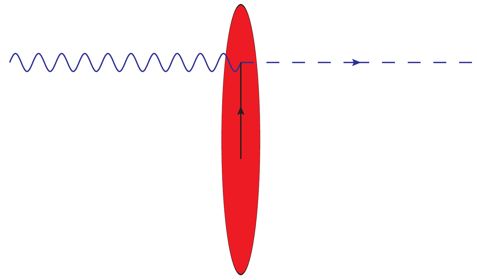
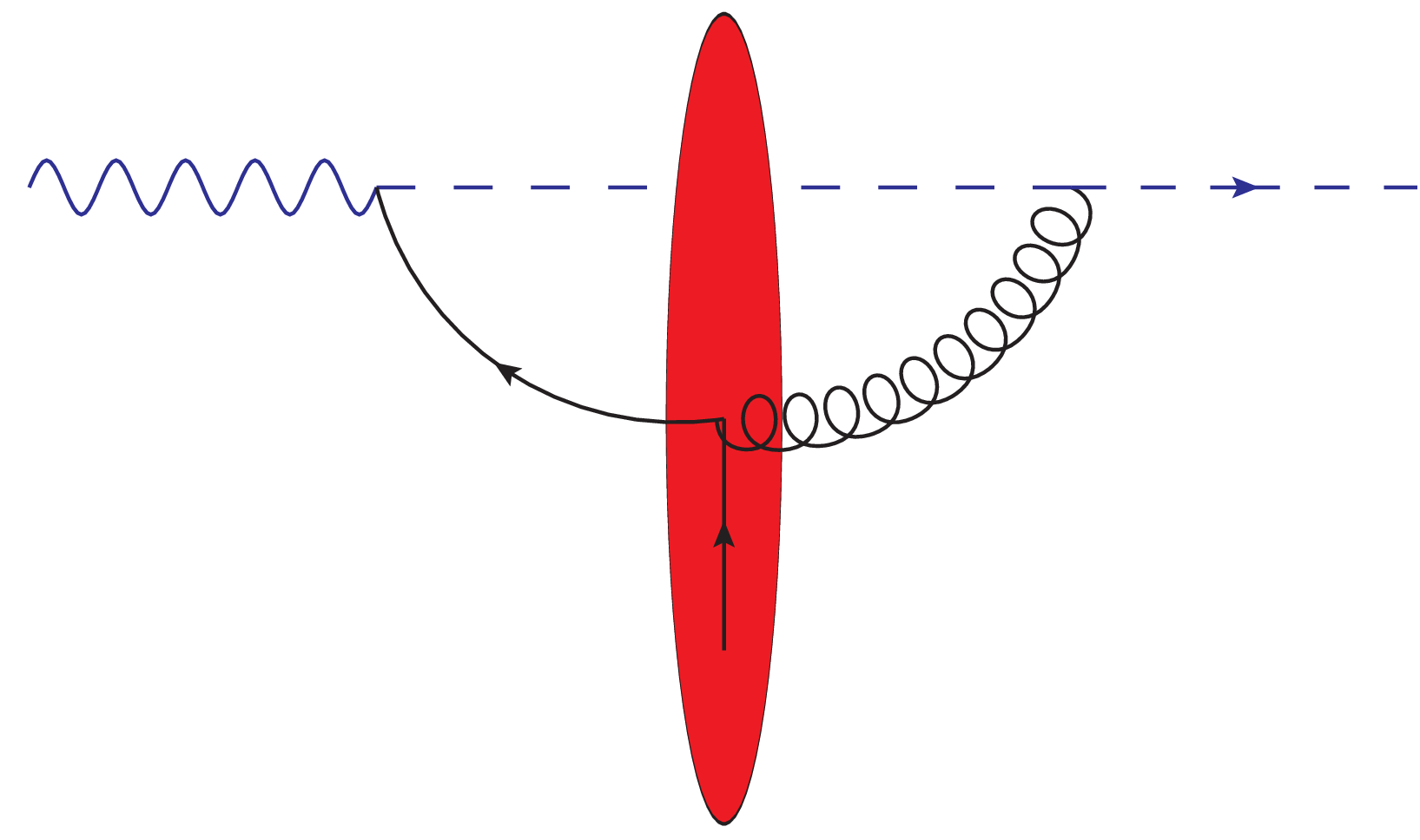
Figure 1: (a) A fast-moving photon interacting with the target quark background field and converting into a fast-moving quark, which is subsequently dressed by eikonal gluon interactions encoded in the shockwave. (b) A diagram contributing to the one-loop corrections to the process..
\[\Psi (z) = \underbrace{\frac{\gamma^+\gamma^-}{2}\Psi(z)}_{ \displaystyle \equiv \Psi^{(-)}(z)} \; + \; \underbrace{\frac{\gamma^-\gamma^+}{2}\Psi(z)}_{ \displaystyle \equiv \Psi^{(+)}(z)} \; ,\] respectively. Under a longitudinal boost of factor \(\gamma_t\) along the \(x^-\) direction, these fields scale as \[\Psi^{(-)}( z ) \propto (\gamma_t)^{1/2}\, ,\Psi^{(+)}( z ) \propto (\gamma_t)^{-1/2}\, .\] Therefore, the leading contribution to quark exchange in the Regge limit is entirely controlled by operators built from \(\Psi^{(-)} (z)\). Moreover, as in the gluon case, at leading eikonal accuracy, the target quark field becomes localized into a shockwave configuration, \[\begin{gather} \Psi^{(-)}(z) = \Psi^{(-)}(z^+, z^-= 0, z_{\perp}) \sim \delta(z^+) \boldsymbol{\Psi}^{(-)} (\boldsymbol{z}) \; , \end{gather}\] reflecting Lorentz contraction along the longitudinal direction.
Guided by the preceding discussion, we seek the simplest Wilson line operator that interpolates a quark propagating eikonally through the target and dressed by an arbitrary number of soft gluon interactions. These requirements motivate the process \(\gamma q\rightarrow \bar q\) illustrated in the left diagram of fig. 1, leading to the operator \[\begin{gather} Q_i(\boldsymbol{z}) = \int dz^+\, [\mathcal{U}_F(\infty^+,z^+,\boldsymbol{z})]_{ij} \, \Psi_j^{(-)}(z^+,\boldsymbol{z}) \; . \label{Eq:AlmostReggeizedQuarkInter} \end{gather}\tag{9}\]
The operator consists of a semi-infinite Wilson line in the fundamental representation starting at the insertion point of the good component of the quark field. The Wilson line resums multiple eikonal interactions of the fast-moving quark with the target gluon background, while the insertion of \(\Psi^{(-)} (z)\) generates the conversion of the projectile into a state carrying \(t\)-channel quark quantum numbers.
Linearizing eq. (9 ) in RGI operators gives \[\begin{gather}
Q_i(\boldsymbol{z})
=
\int
dz^+
\left[
\delta_{ij}
+
ig\,t^a_{ij}
R^a(\infty^+,z^+,\boldsymbol{z})
\right]
\Psi_j^{(-)}(z^+,\boldsymbol{z})
\nonumber
\\ +
\mathcal{O}(g^2R^2)
\equiv
R_{Q,i}(\boldsymbol{z})
+
\mathcal{O}(g^2R^2)\; .
\label{Eq:AlmostReggeizedQuarkInterLinear}
\end{gather}\tag{10}\] The operator \(R_{Q,i}\), therefore, plays for the quark exchange the same role that RGI operator plays for gluon exchange. At leading order it interpolates a free quark state, while
higher-order terms generate an arbitrary number of gluon emissions ordered in light-cone time through the coupling to the Reggeized background field \(R^a\). Eq. (9 ) thus
identifies the minimal Wilson-line operator carrying the color quantum numbers of a Reggeized quark.
As we shall show recovering genuine Regge-pole behaviour requires a projection onto operators of definite signature. To this end, we introduce a signature transformation \(\mathcal{S}\), defined as the reversal of
light-cone time and corresponding to the \(s\leftrightarrow u\)-channel crossing. While the Reggeized gluon interpolating operator in eq. (5 ) is an eigenstate of \(\mathcal{S}\) with eigenvalue \(-1\), the operator obtained from eq. (9 ) is not. Indeed, acting with \(\mathcal{S}\) on its Wilson-line realization, \(Q_i(\boldsymbol{z})\), maps it into \[\begin{gather}
\bar{Q}_i (\boldsymbol{z})
=
\int dz^+\,
[\mathcal{U}_F^{\dagger}(z^+,-\infty^+,\boldsymbol{z})]_{ij}
\,\Psi_j^{(-)}(z^+,\boldsymbol{z})
\nonumber\\
= \int dz^+\,\left[
\delta_{ij}
+
ig\,t^a_{ij}
R^a(-\infty^+,z^+,\boldsymbol{z})
\right] \Psi_j^{(-)}(z^+,\boldsymbol{z}) \nonumber \\
+ \mathcal{O}(g^2 R^2) \equiv
\bar{R}_{Q,i}(\boldsymbol{z})
+ \mathcal{O}(g^2 R^2)\; .
\label{SignatureOperationQuark}
\end{gather}\tag{11}\] This operator corresponds to the crossed-channel configuration \(\bar{q} q\rightarrow \gamma\).
Evolution equation of \(Q_i(\boldsymbol{z})\) and Reggeization in the large-\(N_c\) limit—The rapidity evolution of the operator in eq. (9 ) can be derived within the background-field formalism. At one loop, eikonal power counting allows only one interaction vertex inside the medium (see e.g. Appendix C of ref. [77]). For massless fermions, choosing \(\epsilon_{\rm UV}=\epsilon_{\rm IR}\equiv\epsilon\) removes scaleless external-line
corrections, leaving a single contributing diagram (see (b) in fig. 1).
The derivation of the evolution equation of the operator \(Q_i(\boldsymbol{z}_1)\) is presented in the Supplemantal material. The resulting equation reads \[\begin{gather} \frac{\partial Q_i (\boldsymbol{z}_1)}{ \partial \eta} = (\mu^2)^{1-d/2} \frac{ g^2 }{8 \pi^{1+d}} \left[\Gamma \left( \frac{d}{2} \right) \right]^2 \int d^d \boldsymbol{z}_2 \frac{1}{(\boldsymbol{z}_{12}^2)^{d-1}} \nonumber \\ \times \frac{1}{2} \bigg\{ \left( {\rm Tr}[ \mathcal{U}_F (\boldsymbol{z}_1 ) \mathcal{U}_F^{\dagger} (\boldsymbol{z}_2 )] - \frac{1}{N_c} \right)\delta_{ij} - \nonumber \\ \frac{1}{N_c} \bigg( [ \mathcal{U}_F (\boldsymbol{z}_1 ) \mathcal{U}_F^{\dagger} (\boldsymbol{z}_2 ) ]_{ij} - \delta_{ij} \bigg) \bigg\} Q_j (\boldsymbol{z}_2)\; . \label{Eq:AlmostReggeEvoCoord} \end{gather}\tag{12}\] The relation between eq. (12 ) and quark Reggeization is not immediately apparent at finite \(N_c\). While its interpretation becomes transparent in the planar limit, at finite \(N_c\) a more in depth signature analysis is required.
As a nontrivial consistency check, setting all Wilson lines to the identity reduces eq. (12 ) to the evolution of the good quark component \(\Psi^{(-)} (z)\). After Fourier transformation to momentum space, one recovers the expected evolution governed by the one-loop quark trajectory, \(\delta^{(1)} (-\boldsymbol{p}^2)\), in agreement with the known discontinuity structure of the fixed-order amplitude. We stress that this correspondence is merely a one-loop consistency check and does not constitute a demonstration of all-order Reggeization, whose emergence will be discussed below.
The relation of eq. (12 ) to quark Reggeization becomes immediately transparent in the planar (’t Hooft) limit. In this regime, the second term inside the curly brackets is suppressed, while the dipole operator is \[\begin{gather} {\rm Tr}[ \mathcal{U}_F (\boldsymbol{z}_1 ) \mathcal{U}_F^{\dagger} (\boldsymbol{z}_2 )] = N_c + \mathcal{O}(g^2R^2)\;. \label{Eq:dipoleExp} \end{gather}\tag{13}\] Restricting to the one-Reggeized-gluon sector therefore yields \[\begin{gather} \frac{\partial R_{Q,i} (\boldsymbol{z}_1)}{\partial \eta} = (\mu^2)^{1-d/2} \frac{g^2}{8\pi^{1+d}} \frac{N_c}{2} \left[ \Gamma\left( \frac{d}{2} \right) \right]^2 \nonumber \\ \times \int d^d\boldsymbol{z}_2 \frac{1}{(\boldsymbol{z}_{12}^2)^{d-1}} R_{Q,i}(\boldsymbol{z}_2)\; + \mathcal{O} \left( \frac{1}{N_c} \right) . \end{gather}\]
Comparing with eq. (8 ), one immediately recognizes Regge-pole evolution governed by the trajectory \(\omega^{(1)} (-\boldsymbol{p}^2)/2\), precisely reproducing the large \(N_c\) limit of the quark trajectory in eq. (3 ).
This simplification admits a natural interpretation in terms of signature. Beyond the planar limit, amplitudes with fermion exchange are known to develop singularities more intricate than a simple Regge pole, so that Reggeization is recovered, after
projection onto definite-signature states, in the positive-signature-channel only [12], [13]. In contrast, in the large-\(N_c\) limit the non-planar contributions responsible for this structure are suppressed, and the pole survives already at the level of the non-signaturized
amplitude, leading to an effective degeneracy by signature [12], [13].
Equation (12 ) provides a direct Wilson-line realization of this mechanism: the evolution factorizes into a dipole operator multiplying \(Q_i(\boldsymbol{z})\), and, upon projection
onto the one-Reggeized-gluon sector, the dipole reduces to the identity through eq. (13 ). Quark Reggeization therefore emerges directly, without the need to introduce operators of definite signature.
Signaturization and Reggeization at finite \(N_c\)—We now return to the finite-\(N_c\) case, where the operator \(R_{Q,i}\) cannot be identified as
the Reggeized quark interpolating (RQI), since it does not carry a definite (positive) signature. Indeed, beyond the large-\(N_c\) limit, the second term in the curly brackets contributes already at \(\mathcal{O}(gR)\) in the dilute limit, leading to \[\begin{gather} \frac{\partial R_{Q,i} (\boldsymbol{z}_1)}{ \partial \eta} = \mathcal{K}_{\rm
Regge} (\boldsymbol{z}_{1}, \boldsymbol{z}_{2}) \otimes_{\boldsymbol{z}_2} R_{Q,i} (\boldsymbol{z}_2) \nonumber \\ + [\mathcal{K}_{\rm Non-Regge} (\boldsymbol{z}_{1}, \boldsymbol{z}_{2}) ]_{ij} \;\otimes_{\boldsymbol{z}_2} \bar{R}_{Q,j} (\boldsymbol{z}_2)
\; , \label{Eq:ReggePlusReggeBreak1}
\end{gather}\tag{14}\] where \[\begin{gather} \mathcal{K}_{\rm Regge} (\boldsymbol{z}_{1}, \boldsymbol{z}_{2}) =(\mu^2)^{1-d/2} \frac{g^2 C_F }{8 \pi^{1+d}} \left[\Gamma \left(
\frac{d}{2} \right) \right]^2 \frac{1}{(\boldsymbol{z}_{12}^2)^{d-1}} \; , \label{Eq:KRegge}
\end{gather}\tag{15}\] and \[\begin{gather} [\mathcal{K}_{\rm Non-Regge} (\boldsymbol{z}_{1}, \boldsymbol{z}_{2}) ]_{ij} = (\mu^2)^{1-d/2} \frac{ g^2 }{8 \pi^{1+d}}
\frac{1}{2N_c} \left[\Gamma \left( \frac{d}{2} \right) \right]^2 \nonumber \\ \times \frac{-1}{(\boldsymbol{z}_{12}^2)^{d-1}} igt^a_{ij} \bigg(R^a(\boldsymbol{z}_1) - R^a(\boldsymbol{z}_2) \bigg ) , \label{Eq:KNonRegge}
\end{gather}\tag{16}\] respectively represent the Regge-pole and Regge-pole-breaking parts of the evolution, and we introduced the compact notation \(f(\boldsymbol{z}) \otimes_{\boldsymbol{z}} g(\boldsymbol{z}) =
\int d^d \boldsymbol{z} \; f(\boldsymbol{z}) g (\boldsymbol{z})\).
The structure of eq. (14 ) strongly suggests that the violation of Regge-pole behaviour is tied to the absence of definite signature. First, the evolution couples the operator \(R_{Q,i}\) directly to its \(s\leftrightarrow u\) crossed counterpart \(\bar{R}_{Q,i}\). More importantly, eq. (14 ) possesses a simple transformation property under the signature operation \(\mathcal{S}\): it exchanges \(R_{Q,i}\leftrightarrow \bar{R}_{Q,i}\), leaves \(\mathcal{K}_{\rm Regge}\) invariant, and changes the sign of \(\mathcal{K}_{\rm Non\text{-}Regge}\) as a consequence of the odd signature of the Reggeized gluon interpolating operator entering its definition. This immediately suggests that Regge-pole behaviour can be restored by projecting onto operators of definite signature. Following the standard construction for scattering amplitudes [13], we therefore introduce the positive- and negative-signature combinations
\[\begin{gather} R_{Q,i}^{(\pm)} (\boldsymbol{z}) = \frac{1}{2} \left( R_{Q,i} (\boldsymbol{z}) \pm \bar{R}_{Q,i} (\boldsymbol{z}) \right) = \int d z^+ \, \left[ \frac{\delta_{ij} \pm \delta_{ij}}{2} + ig t^a_{ij} \frac{R^a (\infty^+, z^+ \boldsymbol{z}) \mp R^a ( z^+, -\infty^+, \boldsymbol{z})}{2} \right] \Psi_j^{(-)} (z^+, \boldsymbol{z}) \; , \label{Eq:SignatureProjectionsQuark} \end{gather}\tag{17}\] which are familiar from Regge theory. By using the explicit definition (5 ) and the Baker–Campbell–Hausdorff formula, the sum and difference of the two RGI operators can be related to the logarithm of the product of two semi-infinite Wilson lines \[\begin{gather} R^a (\infty^+, z^+ \boldsymbol{z}) - R^a ( z^+, -\infty^+, \boldsymbol{z}) = \frac{f^{abc}}{g N_c} \bigg[ \ln \left( \mathcal{U}_A (\infty^+, z^+, \boldsymbol{z}) \mathcal{U}_A^{\dagger} (z^+, -\infty^+, \boldsymbol{z} ) \right) \bigg]^{bc} + \mathcal{O} (g^2 R^2) \; , \label{Eq:CBHPositiveSignature} \end{gather}\tag{18}\] \[\begin{gather} R^a (\infty^+, z^+, \boldsymbol{z}) + R^a ( z^+, -\infty^+, \boldsymbol{z}) = \frac{f^{abc}}{g N_c} \bigg[ \ln \left( \mathcal{U}_A (\infty^+, z^+, \boldsymbol{z}) \mathcal{U}_A (z^+, -\infty^+, \boldsymbol{z} ) \right) \bigg]^{bc} + \mathcal{O} (g^2 R^2) = R^a (\boldsymbol{z}) + \mathcal{O} (g^2 R^2) \; , \label{Eq:CBHNegativeSignature} \end{gather}\tag{19}\] neglecting corrections beyond the one-Reggeized-gluon sector. By using eq. (14 ), it is now simple to show that \[\begin{gather} \frac{\partial R_{Q,i}^{(+)} (\boldsymbol{z}_1)}{ \partial \eta} = \mathcal{K}_{\rm Regge} (\boldsymbol{z}_{1}, \boldsymbol{z}_{2}) \otimes_{\boldsymbol{z}_2} R^{(+)}_{Q,i} (\boldsymbol{z}_2) + \mathcal{O} (g^2 R^2)\; , \label{Eq:FinalReggeization} \end{gather}\tag{20}\] and \[\begin{gather} \frac{\partial R_{Q,i}^{(-)} (\boldsymbol{z}_1)}{ \partial \eta} = \mathcal{K}_{\rm Regge} (\boldsymbol{z}_{1}, \boldsymbol{z}_{2}) \otimes_{\boldsymbol{z}_2} R_{Q,i}^{(-)} (\boldsymbol{z}_2) + [\mathcal{K}_{\rm Non-Regge} (\boldsymbol{z}_{1}, \boldsymbol{z}_{2}) ]_{ij} \;\otimes_{\boldsymbol{z}_2} \int d z^+ \Psi_j^{(-)} (z^+, \boldsymbol{z}_2) + \mathcal{O} (g^2 R^2) \; , \label{Eq:NegativeSignatureEvo} \end{gather}\tag{21}\]
which identifies \(R^{(+)}_{Q, i} (\boldsymbol{z})\) as the RQI operator and demonstrates that its rapidity evolution is governed solely by Regge-pole contribution given in eq. 15 . Therefore, the RQI operator admits a clear Wilson-line interpretation: it corresponds to a quark background-field insertion dressed by the logarithm of the product of two semi-infinite Wilson lines defined on a complementary light-cone support.
Eq. (17 ) correctly encodes the perturbative suppression of the negative signature channel, which has no \(\mathcal{O}(g^0)\)-term, with respect to the positive signature one [13]. Remarkably, the negative signature interpolating operator reduces to a product of a Reggeized gluon \(R^a(z)\) times the simple quark insertion. However, the evolution equation of the negative signature part is more complicated, mixing Reggeized quark and Reggeized gluon degrees of freedom (see eq. (16 )). This provides a Wilson-line-based interpretation of the observation made in ref. [13], that the non-Regge pole structure of amplitudes with negative-signature exchange could be explained, in LLA, by branch cuts generated by the exchange of one Reggeized quark plus one Reggeized gluon.
The essence of the present construction is encoded in eqs. (17 –21 ), which single out the Wilson-line operator governing quark exchange in the \(t\)-channel. In particular, eqs. (17 ) and (18 ) identify the Reggeizing operator whose evolution leads to eq. (20 ). This establishes, for the first time, a Wilson-line realization of quark Reggeization in QCD.
Conclusions and outlook—In this Letter, we established a Wilson-line description of quark Reggeization in QCD at LLA. A central obstacle to such a construction has been the intrinsically subeikonal nature of Reggeized quark exchange, whereas
Wilson-line descriptions of high-energy scattering are naturally formulated at eikonal accuracy. Starting from the next-to-eikonal shockwave formalism, we identified a composite operator built from semi-infinite Wilson lines that interpolates the Reggeized
quark and derived its rapidity evolution within the background-field approach. In the dilute limit, its evolution reproduces the characteristic scaling associated with the quark Regge trajectory. In the planar limit, Reggeization emerges already at the
level of the non-signaturized operator, in agreement with the classic observations of Fadin and Sherman. At finite \(N_c\), however, the evolution mixes Reggeized quark and gluon degrees of freedom, and Regge-pole behaviour
is recovered only in the positive-signature sector after projection onto operators of definite signature. These findings demonstrate that quark Reggeization admits a natural realization within the next-to-eikonal sector of the shockwave formalism, thereby
extending the correspondence between Wilson-line evolution and Reggeization established for gluon exchange in ref. [6] to amplitudes
carrying quark quantum numbers in the \(t\)-channel. More broadly, these results provide a first step toward a unified description of high-energy QCD amplitudes from Wilson lines with arbitrary \(t\)-channel quantum numbers.
Several directions naturally emerge from the present work. The most immediate challenge is to determine whether the Wilson-line realization of quark Reggeization extends beyond LLA. Since two-loop rapidity evolution is already known for considerably
more complicated Wilson-line operators [76], [78] (see also [79] for progress at three-loop), the computation of the two-loop quark Regge trajectory and a first-principles derivation of quark Reggeization
at NLLA now appear within reach. More generally, the operator construction developed here can be extended to massive quarks and to channels carrying more general \(t\)-channel color quantum numbers, thereby providing access
to a broader class of high-energy amplitudes. To this aim, one needs to consider a slightly generalized version of the operator in eq. (9 ), where an adjoint Wilson line extends from the insertion point \(z^+\) to \(-\infty^+\). In the present work, we have restricted the discussion to the photon case, which is sufficient to isolate color-triplet exchange and thus the onset of Reggeization.
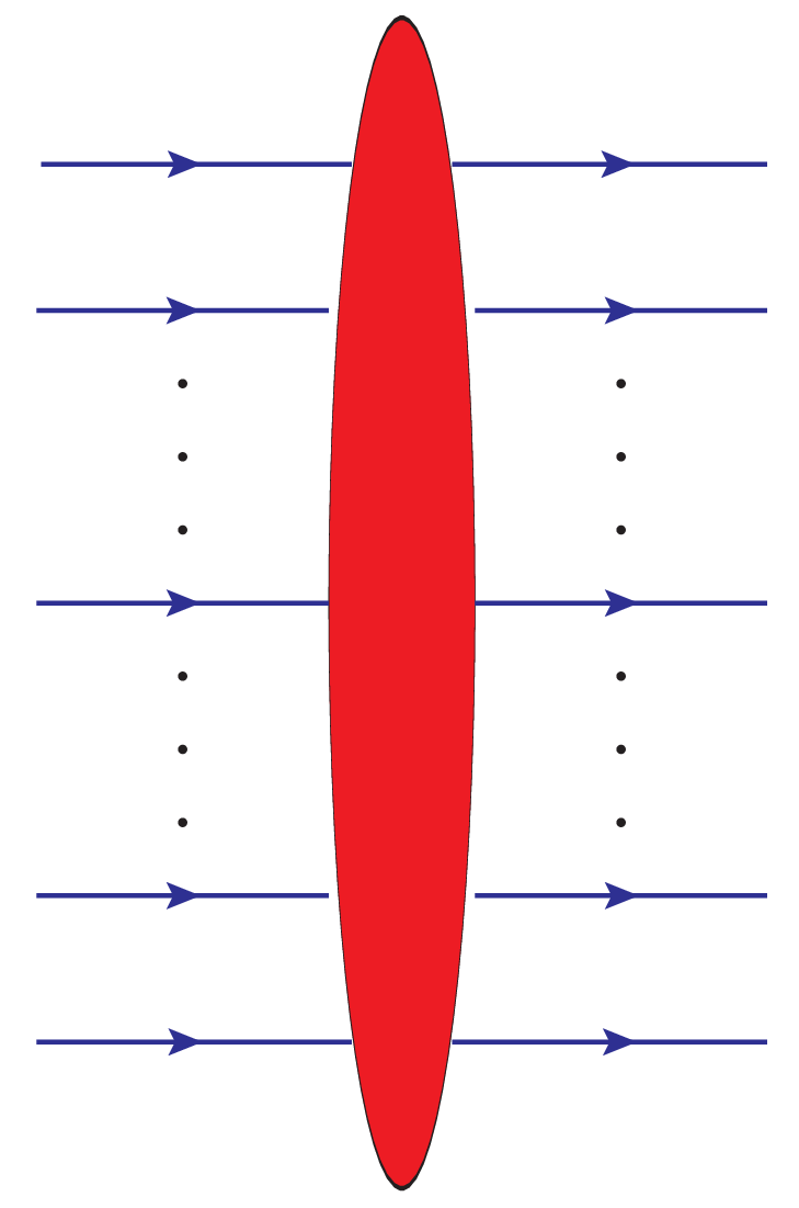
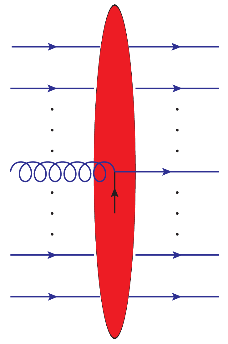
Figure 2: (a) A projectile built from an arbitrary number of Wilson lines in fundamental representation, whose evolution is described by the Balitsky-JIMWLK equation. (b) A projectile in which one constituent (a Wilson line in adjoint representation) changes its nature via subeikonal interactions with the target quark field (to a Wilson line in fundamental representation)..
Finally, the most intriguing direction concerns the role of Regge cuts beyond the regime where Regge-pole dominance holds. In the gluon sector, recent developments suggest that cut contributions can be systematically reconstructed from iterative solutions of the leading-order Balitsky/JIMWLK evolution [6], [57], [60], [63], [64], [69], [70], which governs the rapidity evolution of multi-Wilson-line operators (see diagram (a) in fig. 2). If the correspondence between the Regge structure of high-energy QCD amplitudes and Wilson-line evolution extends beyond the Regge-pole sector, it is natural to expect that a similar connection should emerge also in the quark sector. This points toward a next-to-eikonal extension of the Balitsky hierarchy in which one of the Wilson-line constituents undergoes subeikonal transitions into a quark state through interactions with the target background field (see diagram (b) in fig. 2). Such a framework may ultimately provide access to the all-order structure of quark exchange and multi-Reggeon dynamics, paving the way toward a unified Wilson-line description of high-energy amplitudes beyond the eikonal sector.
Acknowledgments↩︎
We are grateful to R. Boussarie, F. Cougoulic, V. S. Fadin, G. Falcioni, A. Papa, L. Szymanowski, and S. Wallon for insightful discussions. We further thank G. Falcioni and A. Papa for a careful reading of the manuscript. TA and JF are supported in part by the National Science Centre (Poland) under the research Grant No. 2023/50/E/ST2/00133 (SONATA BIS 13). GB is supported in part by the National Science Centre (Poland) under the research Grant No. 2020/38/E/ST2/00122 (SONATA BIS 10). The work of MF is supported by the ULAM fellowship program of NAWA No. BNI/ULM/2024/1/00065 “Color glass condensate effective theory beyond the eikonal approximation”.
Supplemental Materials
1 Derivation of the evolution equations↩︎
In this Supplemental Material, we present the derivations of eqs. (7 ) and (12 ).
1.1 Background field method in the high-energy OPE↩︎
The methodology employed in this work to derive the evolution equations for shockwave operators is based on the high-energy operator product expansion (OPE) introduced by Balitsky [18] in the leading eikonal approximation and more recently extended to next-to-eikonal accuracy in Refs. [73], [80].
For illustration, we briefly review the procedure at leading eikonal accuracy, following closely [81]. Within the shockwave formalism, a
rapidity cut-off \(\eta\) is introduced in order to separate slow (classical) and fast (quantum) degrees of freedom. As in standard renormalization-group approaches, the dependence of the relevant operators on this cut-off
determines their evolution, which in the present case corresponds to the small-\(x\) evolution.
To derive this dependence, one shifts the rapidity cut-off from \(\eta\) to \(\eta+\Delta\eta\) and decomposes the background field as \[\begin{gather}
\mathcal{A}^{-}_{\eta+\Delta\eta}(z)
=
\mathcal{A}^{-}_{\eta}(z)
+
\mathcal{A}^{-}_{\Delta\eta}(z),
\end{gather}\] where the fluctuation field \(\mathcal{A}^{-}_{\Delta\eta}(z)\) contains only gluon modes in the longitudinal momentum interval \(e^\eta p_p^+ < k^+ <
e^{\eta+\Delta\eta} p_p^+\), namely \[\begin{gather}
\mathcal{A}^{-}_{\Delta\eta}(z)
=
\int
\frac{d^Dk}{(2\pi)^D}
e^{-ik\cdot z}
\mathcal{A}^{-}_{\Delta\eta}(k)
\,
\theta(k^+-e^\eta p_p^+)
\theta(e^{\eta+\Delta\eta}p_p^+-k^+).
\end{gather}\] Substituting this decomposition into the Wilson line and expanding in the fluctuation field yields \[\begin{gather} \mathcal{U}_F^{\eta+ \Delta \eta} (x^+, y^+,
\boldsymbol{z}) = \mathcal{U}_F^{\eta} (x^+, y^+, \boldsymbol{z}) + ig \int_{y^+}^{x^+} d z_1^+ \; \mathcal{U}_F^{\eta} (x^+, z_1^+, \boldsymbol{z}) \mathcal{A}^{-}_{\Delta \eta} (z_1^+, \boldsymbol{z} ) \mathcal{U}_F^{\eta} (z_1^+, y^+, \boldsymbol{z})
\nonumber \\ + (ig)^2 \int_{y^+}^{x^+} d z_1^+ \; \int_{y^+}^{z_1^+} d z_2^+ \; \mathcal{U}_F^{\eta} (x^+, z_1^+, \boldsymbol{z}) \mathcal{A}^{-}_{\Delta \eta} (z_1^+, \boldsymbol{z} ) \mathcal{U}_F^{\eta} (z_1^+, z_2^+, \boldsymbol{z})
\mathcal{A}^{-}_{\Delta \eta} (z_2^+, \boldsymbol{z} ) \mathcal{U}_F^{\eta} (z_2^+, y^+, \boldsymbol{z}) \nonumber \\ + \mathcal{O} ((\mathcal{A}_{\Delta \eta}^{-})^2) \; . \label{Eq:ExpansionFluct}
\end{gather}\tag{22}\] where the omitted terms correspond to insertions of more quantum fields \(\mathcal{A}_{\Delta\eta}^-\) along the eikonal trajectory. The evolution equation is then obtained by treating
the modes with \(\displaystyle \ln \left( \frac{k^+}{p_p^+} \right) <\eta\) as a classical external background and integrating over the quantum fluctuations in the rapidity slice \[\eta<\ln
\left( \frac{k^+}{p_p^+} \right) <\eta+\Delta\eta.\] Accordingly, one computes the expectation value of a given operator \(\mathcal{O}\) built from the Wilson lines \[\mathcal{O}^{\eta+\Delta\eta}[\mathcal{U}]= \frac{ \langle0| T\left\{ \mathcal{O}^{\eta}[\mathcal{U}] e^{i\int dz\,\mathcal{L}(z)}
\right\} |0\rangle}{\langle0| T\left( e^{i\int dz\,\mathcal{L}(z)}\right) |0\rangle},\] where the average is taken over the free quantum fields restricted to the rapidity interval \(\Delta\eta\).
In practice, the effect of quantum fluctuations is evaluated through Feynman diagrams involving propagators in the shockwave background. One obtains \[\begin{gather}
\mathcal{O}^{\eta+\Delta\eta}[\mathcal{U}]
=
\mathcal{O}^{\eta}[\mathcal{U}]
+
\Delta\eta\,\mathcal{K}[\mathcal{O}^\eta]
+
\mathcal{O}(\Delta\eta^2),
\end{gather}\] where \[\begin{gather}
\mathcal{K}[\mathcal{O}^\eta]\equiv \frac{I_R+I_V}{\Delta \eta}
\label{Eq:KernelDiagram}
\end{gather}\tag{23}\] is the one-loop evolution kernel. Here, \(I_R\) denotes the real contributions, corresponding to diagrams in which the emitted gluon crosses the shockwave, while \(I_V\) denotes the virtual contributions, corresponding to diagrams without shockwave crossing. Taking the infinitesimal limit in rapidity, one obtains \[\begin{gather}
\frac{\partial}{\partial\eta}
\mathcal{O}^\eta[\mathcal{U}]
=
\lim_{\Delta\eta\to0}
\frac{
\mathcal{O}^{\eta+\Delta\eta}[\mathcal{U}]
-
\mathcal{O}^\eta[\mathcal{U}]
}{\Delta\eta}
=
\mathcal{K}[\mathcal{O}^\eta],
\end{gather}\] which determines the one-loop evolution equation for the operator \(\mathcal{O}^\eta[\mathcal{U}]\).
1.2 Propagators through the Shockwave at the Eik and NEik accuracy↩︎
To calculate the evolution of the operators considered in the present paper, we need a few effective propagators, which we present below.
1.2.0.1 Effective gluon propagator.
The gluon propagator through the Shockwave at the leading-eikonal accuracy is known since the early years of gluon saturation [17]. We present it in mixed momentum-coordinate space representation (see e.g. eq. (2.18) of ref. [82]) \[\begin{gather} G_{\mu \nu}^{ab} (z_1, z_2) = - \frac{(-i)^d}{2 (2 \pi)^{1+d} } \int d^d \boldsymbol{z}_3 [ z_2^+ g_{\perp \mu}^{\alpha} - z_{23 \perp}^{\alpha} n_{2 \mu} ] \mathcal{U}_A^{ab} (\boldsymbol{z}_3) [ -z_1^+ g_{\perp \alpha \nu} - z_{31 \perp \alpha} n_{2 \nu} ] \nonumber \\ \times \int_0^{\infty^+} d k^+ \frac{ (k^+)^{d-1} }{(-z_1^+ z_2^+)^{1+d/2}} e^{i k^+ \left( - z_{21}^{-} + \frac{ \boldsymbol{z}_{23}^2 }{2 z_2^+} - \frac{ \boldsymbol{z}_{31}^2 }{2 z_1^+} + i \varepsilon\right)} \; . \end{gather}\] To derive the evolution equation, we only need propagators constructed from \(\mathcal{A}_{\Delta\eta}^-\), whose interaction with the fast-moving projectile remains purely eikonal, namely \[\begin{gather} G_{\Delta \eta}^{--, ab} (z_1, z_2) = n_{1 \mu} n_{1 \nu} G_{\Delta \eta}^{\mu \nu, ab} = \frac{(-i)^d}{2 (2 \pi)^{1+d} } \int d^d \boldsymbol{z}_3 \; \mathcal{U}_A^{ab} (\boldsymbol{z}_3) \; \boldsymbol{z}_{23} \cdot \boldsymbol{z}_{31} \nonumber \\ \times \int_{e^{\eta} p_p^+}^{e^{\eta + \Delta \eta} p_p^+} d k^+ \frac{ (k^+)^{d-1} }{(-z_1^+ z_2^+)^{1+d/2}} e^{i k^+ \left( - z_{21}^{-} + \frac{ \boldsymbol{z}_{23}^2 }{2 z_2^+} - \frac{ \boldsymbol{z}_{31}^2 }{2 z_1^+} + i \varepsilon\right)} \; . \label{Eq:GluonPropEvoLim} \end{gather}\tag{24}\]
1.2.0.2 Effective antiquark-to-gluon and gluon-to-quark propagators.
The next propagators we present appear in the shockwave formalism at the NEik accuracy and allow identity non-preserving interactions with the target. We will construct them from the expressions of some building-block propagators in Refs. [31] and put them into a form that makes the evolution computation straightforward in coordinate space. Please note that our convention for the
Wilson (see eq. (4 )) differs by a sign with respect to that of Refs. [31]. In deriving these
propagators, as is customary in the Color Glass Condensate framework at subeikonal accuracy, we introduced a finite longitudinal extent \(L^+\) for the target. Ultimately, we are not interested in finite-extent effects,
since they generate only subeikonal corrections; however, keeping \(L^+\) finite at some intermediate steps is useful for providing an intuitive light-cone time picture of the interaction and for the graphical
representation.
Let us first consider the antiquark-to-gluon propagator. It can be written \[\begin{gather} [S^{ \bar{\psi} \rightarrow A } (z_3, z_2) ]_{\mu, l}^{b} = -i g
\int_{-\frac{L}{2}^+}^{\frac{L}{2}^+} d^D z_1 [ S^{b.i.}_{\bar{\psi}} (z_3, z_1) \gamma^{\sigma} t^c \Psi^{(-)} (z_1^+, \boldsymbol{z}_1)]_l [ S^{i.a.}_{A} (z_1, z_2) ]_{\mu \sigma}^{cb} \; , \label{Eq:AntiQuarkGluonPropStart}
\end{gather}\tag{25}\] where we introduced two building-block propagators [31]. The first is the before-to-inside the
medium anti-quark propagator, \(S^{b.i.}_{\bar{\psi}} (z_3, z_1)\), describing an anti-quark starting before the medium, \(z_3^+ < -L^+/2\), and interacting with the quark background
field inside the medium, \(-L^+/2 <z_1^+< L^+/2\) (see the right diagram in fig. 3); it reads \[\begin{gather} S^{b.i.}_{\bar{\psi}} (z_3, z_1) = (-1)
\int \frac{d k_1^+}{(2 \pi)} \frac{d^{d} \boldsymbol{k}_1}{(2 \pi)^d} \frac{\theta (-k_1^+)}{2 k_1^+} e^{-i z_3 \cdot \check{k}_1} (\check{\cancel{k}}_1 + m) \nonumber \\ \times \mathcal{U}_F^{\dagger} ( z_1^+, z_3^+, \boldsymbol{z}_1) \left[ 1 -
\frac{\gamma^+ \gamma^i}{2} i \overleftarrow{D}_{F, \boldsymbol{z}^i} \right] e^{i z_1^- k_1^+ - i \boldsymbol{z}_1 \cdot \boldsymbol{k}_1 } \; ,
\end{gather}\] where we have introduced the vector \(\check{k}_1\) representing the on-shell counterpart of \(k_1\), i.e. \[\begin{gather} k_1^{\mu} =
\check{k}_1^{\mu} + \frac{k_1^2}{2 k_1^+} n_2^{\mu} \; ,
\end{gather}\] and the covariant derivative \[\begin{gather} \overleftarrow{D_{\boldsymbol{z}_1^i}^R} = \overleftarrow{\partial}_{\boldsymbol{z}_1^i} + i g \; T_R \cdot A_i(z_1^+, \boldsymbol{z}_1) \; .
\end{gather}\] The second effective propagator is the before-to-inside-the-medium gluon one, \(S^{i.a.}_{A} (z_1, z_2)\), describing a gluon produced inside the medium (\(-L^+/2
<z_1^+< L^+/2\)) and propagating outside it to the positive light-cone time (\(z_2^+ > L^+/2\)); it reads \[\begin{gather} [S^{i.a.}_{A} (z_1, z_2)]_{\mu \sigma} = \int \frac{d
k_2^+}{(2 \pi)} \frac{d^{d} \boldsymbol{k}_2}{(2 \pi)^d} \frac{\theta (k_2^+)}{2 k_2^+} e^{ - i z_2 \cdot \check{k}_2 } \mathcal{U}^{bc}_A (z_2^+, z_1^+, \boldsymbol{z}_1) \left[ g_{\perp \mu}^{j} - \frac{n_{2 \mu} \boldsymbol{k}_2^j }{ k_2^+ } \right]
\nonumber \\ \times \left[ g_{\perp \sigma}^{j } - \frac{n_{2 \sigma}}{k_2^+} ( i \overleftarrow{D}_{\boldsymbol{z}_1^j}^A + \boldsymbol{k}_2^j ) \right] e^{- i \boldsymbol{k}_2 \cdot \boldsymbol{z}_1 + i k_2^+ z_1^- } \; ,
\end{gather}\] We can simplify the propagator in eq. (25 ) by observing that the term proportional to \(n_{2 \sigma}\) in the \(S^{i.a.}_{A}
(z_1, z_2)\) propagator produces a term proportional to \(\gamma^+ \Psi^{(-)}\), and thus vanishing. After this term disappears, \(\gamma^{\sigma}\) becomes a purely transverse Dirac
matrix, \(\gamma^j\). Then, the term containing \(\gamma^+\) in the \(S^{b.i.}_{\bar{\psi}} (z_3, z_1)\) is also vanishing because \(\gamma^+\) can be moved (apart signs) to produce the vanishing \(\gamma^+ \Psi^ {(-)}\) structure again. In conclusion, all terms containing the covariant derivatives do not contribute, and we
obtain \[\begin{gather} [S^{ \bar{\psi} \rightarrow A } (z_3, z_2) ]_{\mu, l}^{b} = -i g \int \frac{d k^+}{(2 \pi)} \frac{d^{d} \boldsymbol{k}_1}{(2 \pi)^d} \frac{d^{d}
\boldsymbol{k}_2}{(2 \pi)^d} \frac{\theta (k^+)}{4 (k^+)^2} \int_{-\frac{L}{2}^+}^{\frac{L}{2}^+} d z_1^+ d^d \boldsymbol{z}_1 \nonumber \\ \times e^{-i z_3 \cdot \check{k}_1 - i z_2 \cdot \check{k}_2 - i \boldsymbol{z}_1 \cdot ( \boldsymbol{k}_1 +
\boldsymbol{k}_2) } (\check{\cancel{k}}_1 + m) \mathcal{U}_F ( z_3^+, z_1^+, \boldsymbol{z}_1) \gamma^{\sigma} t^c \Psi^{(-)} (z_1^+, \boldsymbol{z}_1) \nonumber \\ \; \times \mathcal{U}_A^{bc} (z_2^+, z_1^+, \boldsymbol{z}_1) \left[ g_{\perp \mu \sigma} -
\frac{n_{2 \mu} \boldsymbol{k}_{2 \sigma} }{ k^+ } \right] , \label{Eq:AntiQuarkGluonPropMiddle}
\end{gather}\tag{26}\] In the present paper, we are considering massless quarks. Moreover, we are only interested in the quantum corrections generating the evolution. For this reason, we can simplify the propagator as
\[\begin{gather} [S_{\Delta \eta}^{ \bar{\psi} \rightarrow A } (z_3, z_2) ]_{l}^{-,b} = i g \int_{e^{\eta}p_p^+}^{e^{\eta+ \Delta \eta} p_p^+} \frac{d k^+}{(2 \pi)}
\frac{d^{d} \boldsymbol{k}_1}{(2 \pi)^d} \frac{d^{d} \boldsymbol{k}_2}{(2 \pi)^d} \frac{\theta (k^+)}{4 (k^+)^3 } \int_{-\frac{L}{2}^+}^{\frac{L}{2}^+} d z_1^+ d^d \boldsymbol{z}_1 \nonumber \\ \times e^{-i z_3 \cdot \check{k}_1 - i z_2 \cdot \check{k}_2 -
i \boldsymbol{z}_1 \cdot ( \boldsymbol{k}_1 + \boldsymbol{k}_2) } \cancel{k}_{1\perp} \cancel{k}_{2 \perp} [\mathcal{U}_F ( z_3^+, z_1^+, \boldsymbol{z}_1) t^c \Psi^{(-)} (z_1^+, \boldsymbol{z}_1 )]_l \mathcal{U}_A^{bc} (z_2^+, z_1^+, \boldsymbol{z}_1) ,
\nonumber \\ \label{Eq:AntiQuarkGluonPropMiddle2}
\end{gather}\tag{27}\] Here, by contracting the propagator with \(n_{2 \mu}\), we immediately impose the eikonal coupling between the gluon and a fast-moving projectile along \(k^+\) and select only the terms containing a rapidity singularity in \(k^+\) (which will generate the leading power in \(\Delta \eta\)). Note that, in order to
do that, one has to neglect both the \(g_{\perp \mu \sigma}\)-term in eq. (26 ) and the \(k^+ \gamma^-\)-term in the \(\cancel{\check{k}}_1\). In all present calculations, we always deal with the case \(\boldsymbol{z}_2 = \boldsymbol{z}_3\), which will be assumed in this derivation. Performing the shifts \[\begin{gather} \boldsymbol{k}_1 \longrightarrow \boldsymbol{k}_1 + \frac{k^+}{z_3^+} \boldsymbol{z}_{12} \; ,\boldsymbol{k}_2 \longrightarrow \boldsymbol{k}_2 - \frac{k^+}{z_2^+} \boldsymbol{z}_{12} \; ,
\end{gather}\] the integrals over \(\boldsymbol{k}_1\) and \(\boldsymbol{k}_2\) becomes Gaussian ones and we obtain \[\begin{gather} [S_{\Delta \eta}^{ \bar{\psi} \rightarrow A } (z_3, z_2) ]_{l}^{-,b} = \frac{g^2}{4 (2 \pi)^{1+d}} \frac{(-i)^{1+d}}{(-z_2^+ z_3^+)^{1+d/2}} \int d^d \boldsymbol{z}_1 \boldsymbol{z}_{12}^2 \int d z_1^+ [\mathcal{U}_F (
- \infty^+, z_1^+, \boldsymbol{z}_1) t^c \Psi^{(-)} (z_1^+, \boldsymbol{z}_1 )]_l \nonumber \\ \times \mathcal{U}_A^{bc} (\infty^+, z_1^+, \boldsymbol{z}_1) \int_{e^{\eta} p_p^+}^{e^{\eta + \Delta \eta} p_p^+} d k^+ (k^+)^{d-1} e^{-i k^+ \left( z_{23}^{-}
- \frac{ \boldsymbol{z}_{12}^2 }{2 z_2^+} + \frac{ \boldsymbol{z}_{12}^2 }{2 z_3^+} + i \varepsilon\right)} \; , \label{Eq:AntiquarkToGluonPropNEik}
\end{gather}\tag{28}\] where we also set \(z_2^+ (z_3^+)\) to \(\infty^+\) (\(-\infty^+\)) inside the Wilson lines, which is always possible
because of the shockwave approximation. Similarly, we extended the integration in \(z_1^+\) to the whole light-cone time.
Another useful result is the “crossed" propagator that is obtained by inverting the direction of the light-cone time, i.e., the effective gluon-to-quark propagator. Similarly to the previous one, it can be constructed from two building-block propagators:
the before-to-inside-the-medium gluon propagator and the inside-to-after-the-medium quark propagator [31]. Because the derivation is
identical to the previous one, we limit ourselves to reporting the final result (in the approximation needed for the evolution): \[\begin{gather} [S_{\Delta \eta}^{A \rightarrow
\psi } (z_3, z_2) ]_{l}^{-,b} = \frac{g^2}{4 (2 \pi)^{1+d}} \frac{- (-i)^{1+d}}{(-z_2^+ z_3^+)^{1+d/2}} \int d^d \boldsymbol{z}_1 \boldsymbol{z}_{12}^2 \int d z_1^+ [\mathcal{U}_F ( \infty^+, z_1^+, \boldsymbol{z}_1) t^c \Psi^{(-)} (z_1^+, \boldsymbol{z}_1
)]_l \nonumber \\ \times \mathcal{U}_A^{bc} (-\infty^+, z_1^+, \boldsymbol{z}_1) \int_{e^{\eta} p_p^+}^{e^{\eta + \Delta \eta} p_p^+} d k^+ (k^+)^{d-1} e^{-i k^+ \left( z_{23}^{-} - \frac{ \boldsymbol{z}_{12}^2 }{2 z_2^+} + \frac{ \boldsymbol{z}_{12}^2 }{2
z_3^+} + i \varepsilon\right)} \; . \label{Eq:GluonToQuarkProp}
\end{gather}\tag{29}\]
1.3 Evolution equations of the Wilson line operators↩︎
Using the propagators introduced in the previous subsection, we can now straightforwardly derive the evolution equations of \(\mathcal{U}_F (\boldsymbol{z})\), \(Q_{i} (\boldsymbol{z})\) and \(\bar{Q}_{i} (\boldsymbol{z})\), presented in the main text.
1.3.0.1 Evolution equation of a single Wilson line.
We start by re-deriving the evolution equation of a single Wilson line that is given in eq. (7 )
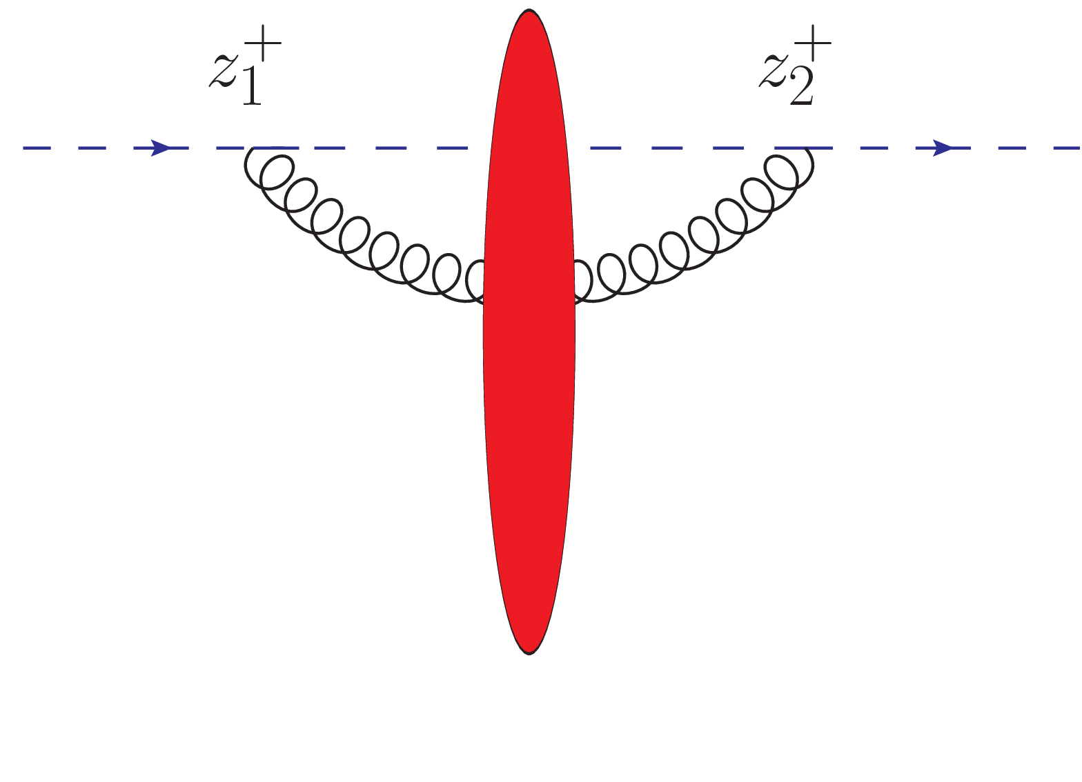
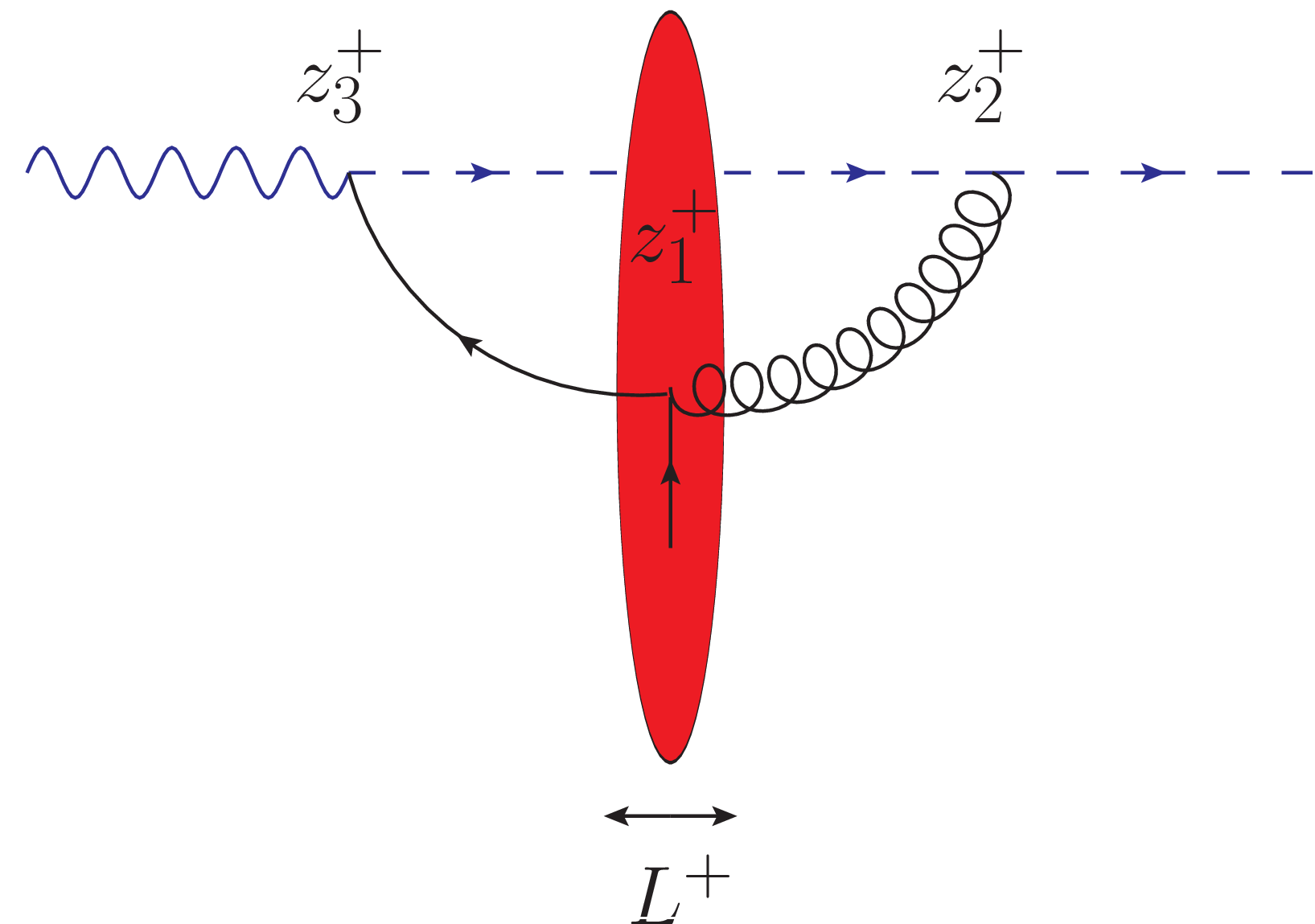
Figure 3: Left: the diagram contributing to the one-loop evolution of a single Wilson line. Right: the diagram contributing to the one-loop evolution of the operator \(Q_i (\boldsymbol{z})\)..
Considering massless external lines, with the choice \(\epsilon \equiv \epsilon_{\rm UV} = \epsilon_{\rm IR}\) to remove scaleless integrals, the expansion (22 ) leads to a single non-vanishing diagram shown in the left diagram of fig. 3. Therefore, to determine \(\mathcal{K}[\mathcal{U}_F (\boldsymbol{z}_1)]\), we compute \[\begin{gather} I_{R} = (\mu^2)^{1-d/2} (i g)^2 \int_{-\infty}^0 d z_1^+ \int_0^{\infty} d z_2^+ [ t^a \mathcal{U}_F (z_2^+, z_1^+, \boldsymbol{z}_1) t^b ]_{ij} n_{1 \mu} n_{1 \nu} G_{\Delta \eta}^{\mu \nu, ab} (z_2^+, z_1^+, \boldsymbol{z}_1) \; . \end{gather}\] The points \(z_1^+\) and \(z_2^+\) can be set to \(-\infty^+\) and \(\infty^+\) in the Wilson lines (including the one in the effective propagators), while the propagator \(G_{\Delta \eta}^{- -, ab} (z_2^+, z_1^+, \boldsymbol{z}_1)\) is obtained from that in eq. (24 ) by setting \(\boldsymbol{z}_1 = \boldsymbol{z}_2\). The integration over the positions \(z_1^+\) and \(z_2^+\) can be performed through the Schwinger formula \[\begin{gather} \int_{0}^{\infty} d \sigma \; \sigma^{d/2 -1} e^{i \sigma A } = \frac{i^{d/2} \Gamma[ \frac{d}{2}]}{A^{d/2}} \; , \label{Eq:SchwingerPar} \end{gather}\tag{30}\] while the integration over \(k^+\) gives \[\begin{gather} \int_{e^{\eta} p_p^+}^{e^{\eta + \Delta \eta} p_p^+} \frac{d k^+}{k^+} e^{-i k^+ ( z_{21}^- - i \varepsilon ) } = \Delta \eta + \mathcal{O} (\Delta \eta^2) \; . \label{Eq:KplusInt} \end{gather}\tag{31}\] After this integration, we obtain \[\begin{gather} I_{R,g} = \frac{\alpha_s (\mu^2)^{1-d/2} [ \Gamma \left( \frac{d}{2} \right)]^2 }{\pi^d} \Delta \eta \int d^d \boldsymbol{z}_3 \frac{1}{(\boldsymbol{z}_{13}^2)^{d-1}} [ t^a \mathcal{U}_F (\boldsymbol{z}_1) t^b ]_{ij} \mathcal{U}_A^{ab} (\boldsymbol{z}_3) \; . \end{gather}\] Using the relation \[\begin{gather} \mathcal{U}_A^{ab} (\boldsymbol{z}_3) t^b = \mathcal{U}_F^{\dagger} (\boldsymbol{z}_3) t^a \mathcal{U}_F (\boldsymbol{z}_3), \label{Eq:FundAdjoi} \end{gather}\tag{32}\] and the Fierz identity \[\begin{gather} t^a_{ik} t^a_{lm} = \frac{1}{2} \left[ \delta_{im} \delta_{lk} - \frac{1}{N_c} \delta_{ik} \delta_{lm} \right] , \end{gather}\] we finally obtain \[\begin{gather} \frac{\partial}{ \partial \eta } [\mathcal{U}_{F} (\boldsymbol{z}_1)]_{ij} = \frac{g^2 }{4 \pi^{1+d}} \left[\Gamma \left( \frac{d}{2} \right) \right]^2 (\mu^2)^{1-d/2} \nonumber \\ \times \int d^d \boldsymbol{z}_{3} \frac{1}{(\boldsymbol{z}_{13}^2)^{d-1}} \frac{1}{2} \left \{ {\rm Tr_c} [\mathcal{U}_{F} (\boldsymbol{z}_1) \mathcal{U}_{F}^{\dagger} (\boldsymbol{z}_3) ] \; [\mathcal{U}_{F} (\boldsymbol{z}_3)]_{ij} - \frac{1}{N_c} [\mathcal{U}_{F} (\boldsymbol{z}_1)]_{ij} \right \} . \label{Eq:SingleWilsonEvoAlm} \end{gather}\tag{33}\] According to our set-up, we can discard the second contribution in the curly bracket of eq. (33 ), which gives rise to scaleless integrals and thus obtain eq. (7 ).
1.3.0.2 Evolution equation of \(Q_i (\boldsymbol{z})\) and \(\bar{Q}_i (\boldsymbol{z})\).
We now consider the evolution equation of the operator \(Q_i (\boldsymbol{z})\), defined in eq. (9 ). To this aim, we just need to compute the right diagram in fig. 1. The starting expression is \[\begin{gather} I_{R, Q} = (\mu^2)^{1-d/2} ( i g ) \int_{-\infty}^0 d z_3^+ \int_0^{\infty} d z_2^+ [ t^b \mathcal{U}_F ( \boldsymbol{z}_2) ]_{il} [S_{\Delta \eta}^{
\bar{\psi} \rightarrow A } (z_3, z_2) ]_{l}^{-, b} \; .
\end{gather}\] We can now substitute the explicit expression of eq. (28 ) and, thanks to the shockwave approximation, set \(z_3^+\) and \(z_2^+\) to \(-\infty^+\) and \(+\infty^+\) in all Wilson lines. Then, the integration over \(z_3^+\) and \(z_2^+\) can be taken through eq. (30 ), while the one over \(k^+\) through eq. (31 ). Moving to the kernel (see eq. 23 ), we obtain \[\begin{gather} \mathcal{K}[Q_i(\boldsymbol{z}_2)] = (\mu^2)^{1-d/2} \frac{ g^2 }{8 \pi^{1+d}} \left[\Gamma \left( \frac{d}{2} \right) \right]^2 \int d^d \boldsymbol{z}_1
\frac{1}{(\boldsymbol{z}_{12}^2)^{d-1}} \nonumber \\ \times \int_{-\frac{L}{2}^+}^{\frac{L}{2}^+} d z_1^+ [ t^b \mathcal{U}_F ( \boldsymbol{z}_2) \mathcal{U}_F (-\infty^+, z_1^+, \boldsymbol{z}_1) t^c \Psi^{(-)} (z_1^+, \boldsymbol{z}_1) ]_{i}
\;\mathcal{U}_A^{cb} (z_1^+, \infty^+, \boldsymbol{z}_1) \; ,
\end{gather}\] which, after using eq. (32 ) and relabeling the transverse integration variable as \(\boldsymbol{z}_2\) and the external integration coordinate \(\boldsymbol{z_1}\), gives \[\begin{gather} \mathcal{K}[Q_i(\boldsymbol{z}_1)] = (\mu^2)^{1-d/2} \frac{ g^2 }{8 \pi^{1+d}} \left[\Gamma \left( \frac{d}{2} \right) \right]^2 \int d^d \boldsymbol{z}_2
\frac{1}{(\boldsymbol{z}^2_{12})^{d-1}} \nonumber \\ \times \frac{1}{2} \bigg \{ \left( {\rm Tr}[ \mathcal{U}_F (\boldsymbol{z}_1 ) \mathcal{U}_F^{\dagger} (\boldsymbol{z}_2 ) ] - \frac{1}{N_c} \right) \delta_{in} - \frac{1}{N_c} \left( [ \mathcal{U}_F
(\boldsymbol{z}_1 ) \mathcal{U}_F^{\dagger} (\boldsymbol{z}_2 ) ]_{in} - \delta_{in} \right) \bigg \} Q_n (\boldsymbol{z}_2) \; .
\end{gather}\] i.e., the evolution kernel on the right-hand side of eq. (12 ).
The evolution of the operator \(\bar{Q}_i (\boldsymbol{z}_1)\) defined in eq. (11 ) is \[\begin{gather} \frac{\partial \bar{Q}_i (\boldsymbol{z}_1)}{ \partial \eta} = (\mu^2)^{1-d/2} \frac{ g^2 }{8 \pi^{1+d}} \left[\Gamma \left( \frac{d}{2} \right) \right]^2 \int d^d \boldsymbol{z}_2
\frac{1}{(\boldsymbol{z}_{12}^2)^{d-1}} \nonumber \\ \times \frac{1}{2} \bigg \{ \left( {\rm Tr}[ \mathcal{U}_F^{\dagger} (\boldsymbol{z}_1 ) \mathcal{U}_F (\boldsymbol{z}_2 ) ] - \frac{1}{N_c} \right) \delta_{in} - \frac{1}{N_c} \left( [
\mathcal{U}_F^{\dagger} (\boldsymbol{z}_1 ) \mathcal{U}_F (\boldsymbol{z}_2 ) ]_{in} - \delta_{in} \right) \bigg \} \bar{Q}_n (\boldsymbol{z}_2) \; . \label{Eq:EvoOfcrossedOperator}
\end{gather}\tag{34}\] The eq. (34 ) can be obtained both by explicitly computing the crossed version of the left diagram in fig. 1 (by means of the effective
propagator in eq. (29 )), or by applying the signature transformation \(\mathcal{S}\) (i.e. \(\infty^+ \leftrightarrow -\infty^+\) transformation).