1 Introduction↩︎

A central goal of modern quantum physics is efficient manipulation of the interaction between quantum emitters (QEs) and a quantized electromagnetic (EM) field. This is of particular importance for constructing large-scale quantum networks [1], [2] where the evolution and interaction of its constituents can be controlled at the quantum level. The elementary process of constituents is the interaction between a single photon and a single QE. In free space, the QE-field coupling leads to an excited QE unavoidably decaying towards its ground state by emitting a single photon to any of a continuum characterized by different wave vectors. Boundaries and artificial dimensional reduction tailor the mode density of the electromagnetic field, spontaneous emission is either enhanced, inhibited or even completely hindered[3]–[6]. In this context, cavity QED [7] setups have been extensively studied due to the confinement of light into smaller volumes resulting in the strong enhancement of single QE coupling to one preferred mode and/or suppression of the coupling to all unwanted modes. In parallel to these cavity-based settings, the coupling of QEs to waveguides, called waveguide-QED system, has also raised a large interest as it enables the strong interaction of a single or multiple atoms with a guided mode [8]–[10]. QEs coupled with the 1D waveguides behave as a gate for photons fly in the 1D waveguide, such as single-photon switches[11]–[13], routers[14]–[21], and frequency converters[22]–[25].

With the great technological progress to the chip scale, the waveguide-QED system has been generalized to studies of a QE nonlocally coupled to photons in the waveguide[26], [27]. QEs with dimension comparable to or larger than the wavelength of its emitted photon are called giant atom (GA)[28]–[36]. One of the paradigmatic models is a single GA coupled to a waveguide at multiple spatially separated points. A hallmark of GA-waveguide system is the nonexponential atomic decay, a non-Markovian character, due to the self-interference effect induced by the separated coupling points, which has been manifested in the form of dressed atom-photon bound states [37]–[44] and experimentally demonstrated with superconducting qubits coupled to surface acoustic waves [45]. And the engineered complex phases in the atom-light couplings [46], which determines the chirality of a GA [47], leads to nonreciprocal transport of photons [48] and a preferred direction of emitted radiation. In this paper, we consider a \(\Lambda\)-type GA whose both transitions are coupled to a waveguide at two spatially separated points. A three-level emitter (3LE) is more suitable for long-lived information storage in comparison with the two-level emitter (2LE), since it transfers the coherence of light into the coherence between ground states. We concentrate on the spontaneous emission of this three-level giant atom (3GA) in single excitation of this system. A delay-differential equation for the amplitude of the 3GA in its excited state is followed from the Schrodinger equation to describe the self-interference with the waveguide by virtual photon exchanges. A photonic bound state can be formed in a continuum produced by the destructive interference effects by tuning the distance between the coupling points or the energy spacing when the distance of the two coupling points is smaller or comparable to the coherent length characterizing the width of the emitted wave packet. The formation of the photonic bound state leads to a departure from the exponential decay, a presentation of a non-Markovian character. We also show that the 3GA can exhibit exact Markovian dynamics via the interference between two propagating channels for photons even for non-negligible time delays in addition to tuning the complex phases in the atom-light couplings.

2 A GA Coupled to A 1D Waveguide↩︎

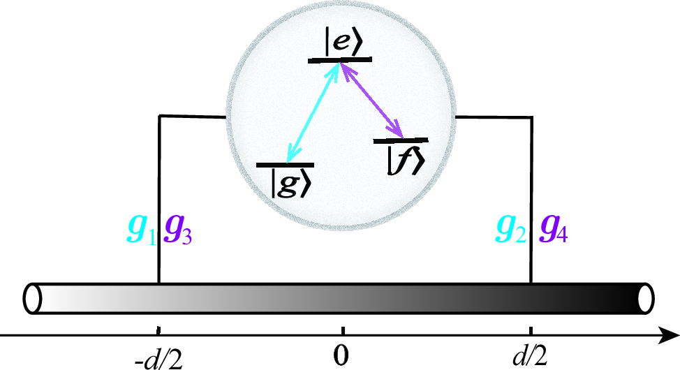
We consider a 3GA in a so-called \(\Lambda\) scheme with the upper level \(\left\vert e\right\rangle\), two lower levels \(\left\vert g\right\rangle\) and \(\left\vert f\right\rangle\) separated by the transition frequencies \(\omega _{e}\) and \(\omega _{ef}=\omega _{e}-\omega _{f}\), respectively, as shown in the schematic Fig. 1. Note that \(\omega _{e}-\omega _{ef}=\omega _{f}\) is the frequency separation of the lower levels with its ground energy being set to zero. The upper level \(\left\vert e\right\rangle\) is coupled to lower levels \(\left\vert g\right\rangle\) and \(\left\vert f\right\rangle\) by the same vacuum modes of a one-dimensional (1D) waveguide at position \(x=-d/2\) and \(d/2\). The waveguide supports a continuum of electromagnetic modes, each with associated frequency \(\omega\). Its 1D continuum is formed by the right-going and left-going modes, the right-going mode are represented by the canonical creation and annihilation operators \(\hat{r}_{\omega }^{\dagger }\) and \(\hat{r}_{\omega }\), and the left-going mode are represented by \(\hat{l}_{\omega }^{\dagger }\) and \(\hat{l}_{\omega }\). Both modes obey the bosonic commutation relation \([\alpha _{\omega },\alpha _{\omega ^{\prime }}^{\dagger }]=\delta (\omega -\omega ^{\prime })\) with \(\alpha =\hat{r}_{\omega },\hat{l}_{\omega }\). The total GA-waveguide Hamiltonian can be written as \(\hat{H}=\hat{H}_{A}+\hat{H}_{W}+\hat{H}_{I}\), where \[\hat{H}_{A}=\omega _{f}\hat{\sigma}_{ff}+\omega _{e}\hat{\sigma}_{ee} \label{sec2-1}\tag{1}\] is the Hamiltonian for the GA and atomic operator \(\hat{\sigma}_{\beta \beta ^{\prime }}=\left\vert \beta \right\rangle \left\langle \beta ^{\prime }\right\vert\) with \(\beta ,\beta ^{\prime }\in \left\{ g,f,e\right\}\). The free evolution of the quantized radiation field inside the waveguide is described by \[\hat{H}_{W}=\int_{0}^{\infty }d\omega \omega \left( \hat{r}_{\omega }^{\dagger }\hat{r}_{\omega }+\hat{l}_{\omega }^{\dagger }\hat{l}_{\omega }\right) .\]By neglecting counter-rotating terms, the interaction of the GA with the waveguide reads\[\begin{align} \hat{H}_{I} &=&\frac{1}{\sqrt{\upsilon _{g}}}\int_{0}^{\infty }d\omega \left( g_{1}e^{-\mathrm{i}\frac{\omega \tau }{2}}+g_{2}e^{\mathrm{i}\frac{\omega \tau }{2}}\right) \hat{r}_{\omega }^{\dagger }\hat{\sigma}_{ge}+H.c. \label{sec2-2} \\ &&+\frac{1}{\sqrt{\upsilon _{g}}}\int_{0}^{\infty }d\omega \left( g_{3}e^{-\mathrm{i}\frac{\omega \tau }{2}}+g_{4}e^{\mathrm{i}\frac{\omega \tau }{2}}\right) \hat{r}_{\omega }^{\dagger }\hat{\sigma}_{fe}+H.c. \notag \\ &&+\frac{1}{\sqrt{\upsilon _{g}}}\int_{0}^{\infty }d\omega \left( g_{1}e^{\mathrm{i}\frac{\omega \tau }{2}}+g_{2}e^{-\mathrm{i}\frac{\omega \tau }{2}}\right) \hat{l}_{\omega }^{\dagger }\hat{\sigma}_{ge}+H.c. \notag \\ &&+\frac{1}{\sqrt{\upsilon _{g}}}\int_{0}^{\infty }d\omega \left( g_{3}e^{\mathrm{i}\frac{\omega \tau }{2}}+g_{4}e^{-\mathrm{i}\frac{\omega \tau }{2}}\right) \hat{l}_{\omega }^{\dagger }\hat{\sigma}_{fe}+H.c. \notag \end{align}\tag{2}\] where \(g_{j}\) are GA-waveguide coupling strengths and \(\tau =d/\upsilon _{g}\) is delay time that the light emitted from the GA into the waveguide travels along the distance between two coupling points. As the total number of excitations is preserved in this system, the subspace without excitations is two-dimensional and is spanned by the bare states \(\left\{ \left\vert 0g\right\rangle ,\left\vert 0f\right\rangle \right\}\) with \(\left\vert 0\right\rangle\) being the vacuum state of the field. In the single-excitation subspace, the state at time \(t\) is a superposition of a photon moving to the right or the left with the GA in any of the lower state, and the GA is in the excited state \[\begin{align} \vert \Psi(t) \rangle &= \sum_{\beta=g,f} \int_{0}^{\infty} d\omega \, \psi_{\beta l\omega}(t) \, l_{\omega}^{\dagger} \vert 0\beta \rangle + u(t) \vert 0e \rangle \\ &\quad + \sum_{\beta=g,f} \int_{0}^{\infty} d\omega \, \psi_{\beta r\omega}(t) \, r_{\omega}^{\dagger} \vert 0\beta \rangle \end{align} \label{sec2-3}\tag{3}\] Here, \(u\left( t\right)\) is the excited amplitude, and \(\psi _{\beta r\omega }\left( t\right)\) (\(\psi _{\beta l\omega }\left( t\right)\)) are right- and left-moving field amplitudes with frequency \(\omega\) while the GA is in the state \(\left\vert \beta \right\rangle\). The Schrödinger equation transforms \(\left\vert \Psi \left( t\right) \right\rangle\) into coupled equations of motion for the amplitudes \[\label{sec2-4}\begin{align} \dot{\psi}_{gl\omega}\left( t\right) & =-\mathrm{i}\omega\psi_{gl\omega }\left( t\right) -\mathrm{i}\frac{u\left( t\right) }{\sqrt{\upsilon_{g}}}\left( g_{1}e^{\mathrm{i}\frac{\omega\tau}{2}}+g_{2}e^{-\mathrm{i}\frac{\omega\tau}{2}}\right) \\ \dot{\psi}_{gr\omega}\left( t\right) & =-\mathrm{i}\omega\psi_{gr\omega }\left( t\right) -\mathrm{i}\frac{u\left( t\right) }{\sqrt{\upsilon_{g}}}\left( g_{1}e^{-\mathrm{i}\frac{\omega\tau}{2}}+g_{2}e^{\mathrm{i}\frac{\omega\tau}{2}}\right) \\ \dot{\psi}_{fl\omega}\left( t\right) & =-\mathrm{i}\left( \omega _{f}+\omega\right) \psi_{fl\omega}\left( t\right) -\mathrm{i}\frac{u\left( t\right) }{\sqrt{\upsilon_{g}}}\left( g_{3}e^{\mathrm{i}\frac{\omega\tau}{2}}+g_{4}e^{-\mathrm{i}\frac{\omega\tau}{2}}\right) \nonumber\\ & \\ \dot{\psi}_{fr\omega}\left( t\right) & =-\mathrm{i}\left( \omega _{f}+\omega\right) \psi_{fr\omega}\left( t\right) -\mathrm{i}\frac{u\left( t\right) }{\sqrt{\upsilon_{g}}}\left( g_{3}e^{-\mathrm{i}\frac{\omega\tau }{2}}+g_{4}e^{\mathrm{i}\frac{\omega\tau}{2}}\right) \nonumber\\ & \\ \dot{u}\left( t\right) & =-\mathrm{i}\omega_{e}u\left( t\right) -\int_{0}^{\infty}d\omega\left( g_{1}^{\ast}e^{\mathrm{i}\frac{\omega\tau}{2}}+g_{2}^{\ast}e^{-\mathrm{i}\frac{\omega\tau}{2}}\right) \frac{\mathrm{i}\psi_{gr\omega}\left( t\right) }{\sqrt{\upsilon_{g}}}\nonumber\\ & -\int_{0}^{\infty}d\omega\left( g_{1}^{\ast}e^{-\mathrm{i}\frac{\omega\tau }{2}}+g_{2}^{\ast}e^{\mathrm{i}\frac{\omega\tau}{2}}\right) \frac{\mathrm{i}\psi_{gl\omega}\left( t\right) }{\sqrt{\upsilon_{g}}}\nonumber\\ & -\int_{0}^{\infty}d\omega\left( g_{3}^{\ast}e^{\mathrm{i}\frac{\omega\tau }{2}}+g_{4}^{\ast}e^{-\mathrm{i}\frac{\omega\tau}{2}}\right) \frac{\mathrm{i}\psi_{fr\omega}\left( t\right) }{\sqrt{\upsilon_{g}}}\nonumber\\ & -\int_{0}^{\infty}d\omega\left( g_{3}^{\ast}e^{-\mathrm{i}\frac{\omega\tau }{2}}+g_{4}^{\ast}e^{\mathrm{i}\frac{\omega\tau}{2}}\right) \frac{\mathrm{i}\psi_{fl\omega}\left( t\right) }{\sqrt{\upsilon_{g}}}\end{align}\tag{4}\]

3 Atomic dynamics↩︎

In this section we investigate the spontaneous emission of the GA initially prepared in the excited state, i.e., the initial state is \(\left\vert \Psi \left( 0\right) \right\rangle =\left\vert 0e\right\rangle\). By formally integrating the equations for \(\psi _{\beta r\omega }\left( t\right)\) and \(\psi _{\beta l\omega }\left( t\right)\) with intial \(\psi _{\beta r\omega }\left( 0\right) =\psi _{\beta l\omega }\left( 0\right) =0\) and inserting them into the Eq.(4 e), the photonic degree of freedom can be completely eliminated, yielding a delay-differential equation \[\begin{align} \dot{U}\left( t\right) &=&-\left( \frac{\Gamma _{g}}{2}+\frac{\Gamma _{f}}{2}\right) U\left( t\right) \label{sec3-01} \\ &&-\left( \frac{\gamma _{g}}{2}e^{\mathrm{i}\varphi _{g}}+\frac{\gamma _{f}}{2}e^{\mathrm{i}\varphi _{f}}\right) U\left( t-\tau \right) \notag \end{align}\tag{5}\] where we have introduced \(u\left( t\right) =U\left( t\right) e^{-\mathrm{i}\omega _{e}t}\), \(\Theta \left( t\right)\) is the Heaviside step function, and \[\label{sec3-02} \begin{eqnarray} \Gamma _{g} &=&\frac{2\pi }{\upsilon _{g}}\left( \left\vert g_{1}\right\vert ^{2}+\left\vert g_{2}\right\vert ^{2}\right) , \gamma _{g} =\frac{4\pi }{\upsilon _{g}}\left\vert g_{1}\right\vert \left\vert g_{2}\right\vert \cos \phi _{g}, \\ \Gamma _{f} &=&\frac{2\pi }{\upsilon _{g}}\left( \left\vert g_{3}\right\vert ^{2}+\left\vert g_{4}\right\vert ^{2}\right) , \gamma _{f} =\frac{4\pi }{\upsilon _{g}}\left\vert g_{3}\right\vert \left\vert g_{4}\right\vert \cos \phi _{f}. \end{eqnarray}The first term on the right hand side of Eq.(\ref{sec3-01}) corresponds to the usual free space exponential decay with rate \Gamma _{\alpha } to the continua \hat{l}_{\omega }^{\dagger }\left\vert 0\alpha \right\rangleand \hat{r}_{\omega }^{\dagger }\left\vert 0\alpha \right\rangle , which are referred to as g-channel and f-channel, respectively. The second term represents the effect of the retarded radiation on the GA that was emitted at time \taubefore it interacts again with the GA. Here, the emission field of the GA acquires phases \theta _{j}=\arg g_{j}, j\in \left\{ 1,2,3,4\right\}at the coupling points generating the phase difference \phi _{g}=\theta _{1}-\theta_{2} and \phi _{f}=\theta _{3}-\theta _{4} , and accumulates propagation phases \varphi _{g}=\omega _{e}\tauor \varphi _{f}=\omega _{ef}\tauwhen light propagates from one coupling point to its adjacent coupling point via g-channel or f-channel. The time-dependent excited amplitude in Eq.(\ref{sec3-01}) can be calculated by standard Laplace equations:\tag{6}\] \[U\left( t\right) =\int \frac{e^{st}ds/\left( 2\pi \mathrm{i}\right) }{s+\frac{\Gamma }{2}+\frac{1}{2}\left( \gamma _{g}e^{\mathrm{i}\varphi _{g}}+\gamma _{f}e^{\mathrm{i}\varphi _{f}}\right) e^{-s\tau }} \label{sec3-03}\tag{7}\] with the total decay rate \(\Gamma =\Gamma _{g}+\Gamma _{f}\) and \(s\) the complex frequency parameter of the Laplace transformation. In the case of \(\tau \rightarrow \infty\) or \(g_{1}\left( g_{2}\right) =0\) and \(g_{3}\left( g_{4}\right) =0\), the system becomes a pointlike 3LE interacting with a waveguide. When \(g_{1}=g_{2}=0\) or \(g_{3}=g_{4}=0\), the 3GA reduces to a 2GA where the \(g\)-channel or \(f\)-channel disappears, and the 2GA further reduces to a point-like 2LE when \(g_{3}(g_{4})=0\) or \(g_{1}(g_{2})=0\).

Using geometric series expansion as \(\gamma _{\beta }\leq \Gamma _{\beta }\) with \(\beta \in \left\{ g,f\right\}\), the inverse Laplace transform yields the time-dependent amplitudes \[U\left( t\right) =\sum_{n=0}^{\infty }\frac{\left( -1\right) ^{n}}{2^{n}n!}\left( \gamma _{g}e^{\mathrm{i}\varphi _{g}}+\gamma _{f}e^{\mathrm{i}\varphi _{f}}\right) ^{n}t_{n}^{n}e^{-\frac{\Gamma }{2}t_{n}}\Theta \left( t_{n}\right) \label{sec3-04}\tag{8}\] where \(t_{n}=t-n\tau\). Eq.(8 ) has a ” step”character if the time axis is divided into intervals of length \(\tau\). For the \(n=0\) interval \(t\in \left[ 0,\tau \right]\), the sum consists only of one term, \(\exp \left( -\Gamma t/2\right)\), coincides with the behavior of a pointlike 3LE decaying to a 1D waveguide since the emitted photon requires at least the time \(\tau\) to travel between adjacent coupling points. For \(t\in \left[ \tau ,2\tau \right]\), the amplitude consists of three terms since \(n=1\) interval in Eq.(8 ) is included, which give rise to interference in the atomic population due to the emitted radiation absorbed by the GA at the coupling point. And the propagation of the emitted photon along \(g\)- and \(f\)-channel leads to the dynamics of the GA strongly dependent on the propagating phases \(\varphi _{g}\) and \(\varphi _{f}\). For longer times, more terms from the series expansion (8 ) contribute to the dynamics.

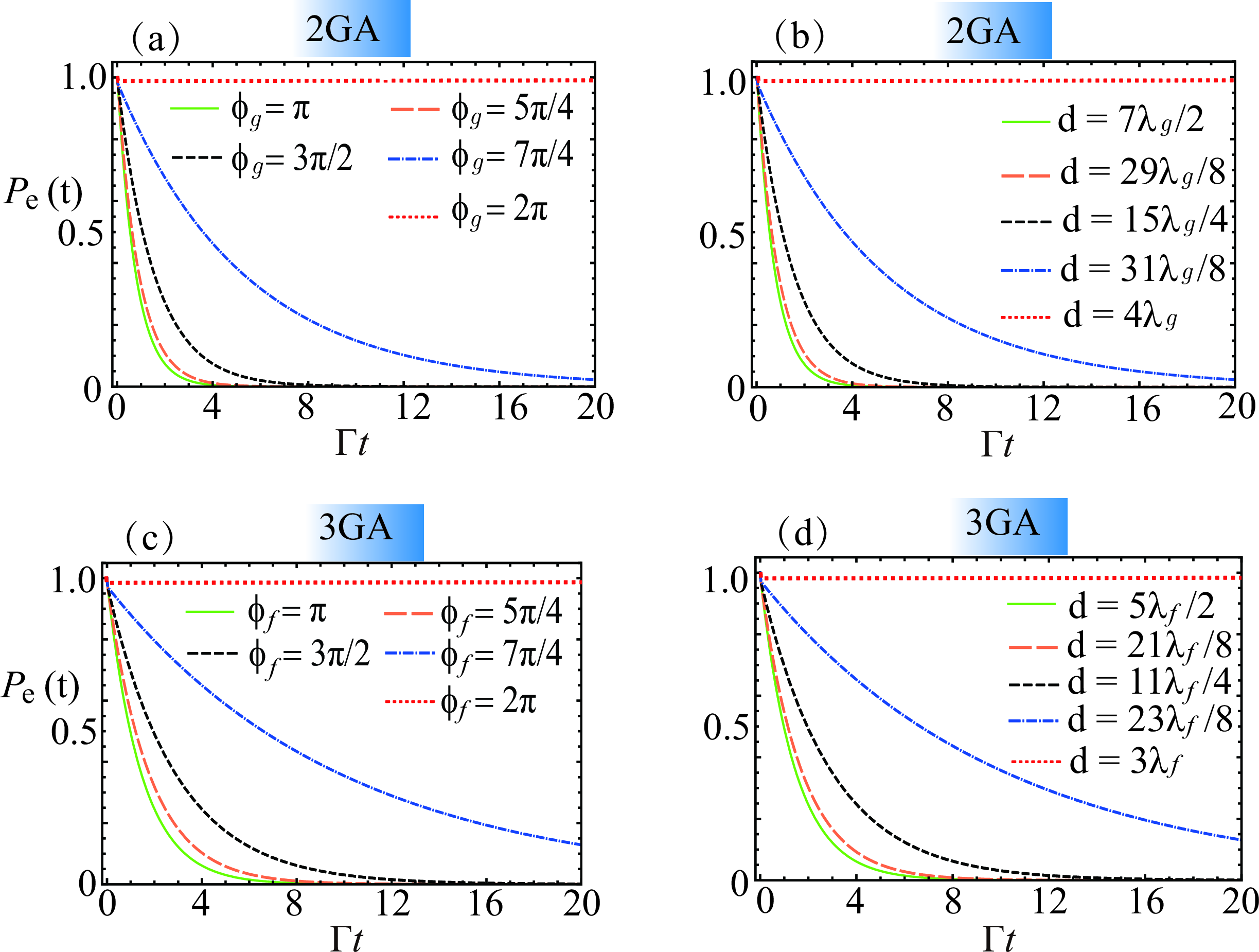
The role of the interference terms strongly depends on the distance \(d\) between the coupling points, the wavenumbers \(\lambda _{g}=2\pi \upsilon _{g}/\omega _{e}\) and \(\lambda _{f}=2\pi \upsilon _{g}/\omega _{ef}\), and the coherence length \(L=\upsilon _{g}/\Gamma\) describing the width of the emitted wave packet. For GAs, \(\lambda _{\beta }<d,L\) is usually satisfied. In Fig.2, we have plotted the probabilities \(P_{e}\left( t\right) =\left\vert u\left( t\right) \right\vert ^{2}\) in the excited state as a function of the scaled time \(\Gamma t\) in the short delay case under the condition \(\left\vert g_{1}\right\vert =\left\vert g_{2}\right\vert\) and \(\left\vert g_{3}\right\vert =\left\vert g_{4}\right\vert\). The short delay case corresponds to \(d\ll L\), i.e., the time it takes for the GA to completely decay to its two lower states is longer than the delay time. In this context, the factor \(e^{-s\tau }\approx 1\) in Eq.(7 ), so a Markovian approximation can be made. The exponential decay curves is usually associated with the Markovian approximation. To show the difference of the 2GA and the 3GA, we set \(g_{3}=g_{4}=0\) in Fig.2 (a,b). The behavior of the black dashed line with \(\phi _{g}=\left( n+1/2\right) \pi\) in Fig.2 (a) and \(d=\left( n\pm 1/4\right) \lambda _{g}\) (i.e., \(\varphi _{g}=\left( 2n\pm 1/2\right) \pi\)) in Fig.2 (b) is the same to the exponential decay of the 2LE coupled to a 1D waveguide. The decay is either enhanced or slowed down depending on the values of the parameters. The decay vanishes at \(\phi _{g}=2n\pi\) (\(\left( 2n+1\right) \pi\)) and \(\varphi _{g}=\left( 2n+1\right) \pi\) (\(2n\pi\)), and maximizes at \(\phi _{g}=\left( 2n+1\right) \pi\) (\(2n\pi\)) and \(\varphi _{g}=\left( 2n+1\right) \pi\) (\(2n\pi\)), see the red dotted lines and the green solid line in Fig.2 (a,b) respectively. The red dotted lines manifest a trapping of the excitation in the 2GA. In Fig.2 (c,d), we have fixed \(\phi _{g}=2\pi\) and \(\varphi _{g}=\left( 2n+1\right) \pi\) corresponding to complete suppression of the spontaneous emission of the 3GA via the g-channel, see the red dotted lines in Fig.2 (a). By allowing the transition \(\left\vert e\right\rangle \leftrightarrow \left\vert f\right\rangle\), the decay is generally enhanced, and the behavior of the black dashed curves with \(\phi _{f}=3\pi/2\) in Fig.2 (c) and \(d=\left( n\pm 1/4\right) \lambda _{f}\) (i.e., \(\varphi _{f}=\left( 2n\pm 1/2\right) \pi\)) in Fig.2 (d) is the same to the exponential decay of the 2LA with transition \(\left\vert e\right\rangle\) and \(\left\vert f\right\rangle\) coupled to a 1D waveguide. The decay maximizes at \(\phi _{f}=\left( 2n+1\right) \pi\) (\(2n\pi\)) and \(\varphi _{f}=\left( 2n+1\right) \pi\) (\(2n\pi\)), see the green solid curves. A trapping of the excitation in the excited state of the 3GA appears at \(\phi _{f}=2n\pi\) (\(\left( 2n+1\right) \pi\)) and \(\varphi _{f}=\left( 2n+1\right) \pi\) (\(2n\pi\)), see the red dotted curves. In contrast to the 3GA with external driving field in Ref.[43], [44], the population trapping of the excitation is manifested only in the form of a residual non-vanishing constant in the long enough time.

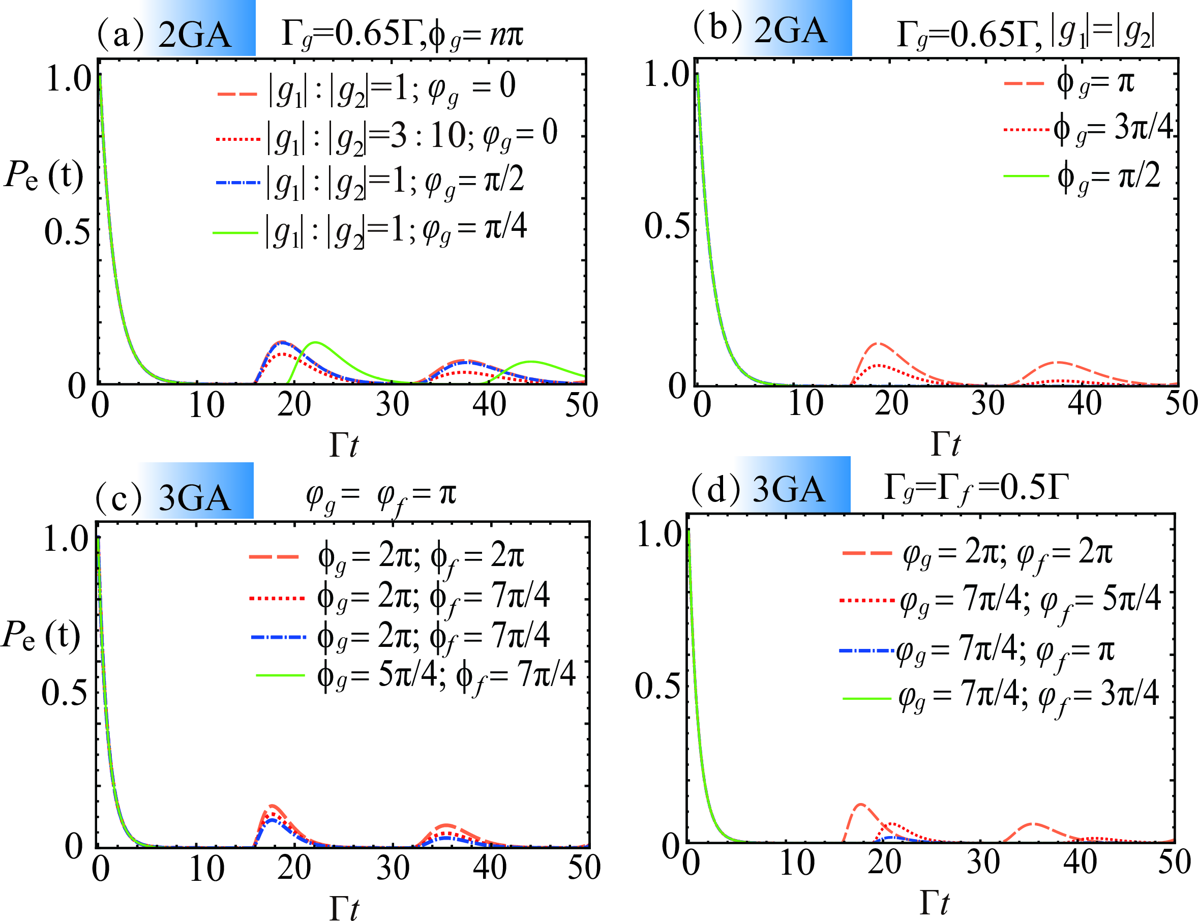
As the length of the distance of the coupling points grows such that \(d\gg L\), the lifetime \(\Gamma ^{-1}\) associated with the exponential decay factor on each time interval is short compared with the duration \(\tau\) of each interval, the contributions from different intervals do not appreciably overlap. In this long delay case, the probability reads \[P_{e}\left( t\right) \approx \frac{1}{2^{2n}n!^{2}}\left\vert \gamma _{g}+\gamma _{f}e^{\mathrm{i}\left( \varphi _{f}-\varphi _{g}\right) }\right\vert ^{2n}t_{n}^{2n}e^{-\Gamma t_{n}} \label{sec3-05}\tag{9}\] in the \(n\)th time interval. It is possible for the GA to be partially re-excited by the radiation which it has emitted before. Figure 3 shows the probability \(P_{e}\left( t\right)\) in the long delay case. The exponential decay in the first interval (\(0\leq t\leq \tau\)) is followed by a recurrence of probability beginning at \(t=\tau\). The probability peaks at \(t=n\left( \tau +2/\Gamma \right)\) and reaches a peak value at \[P_{e}\left( t\right) =\frac{1}{n!^{2}}\left\vert n\frac{\gamma _{g}+\gamma _{f}e^{\mathrm{i}\left( \varphi _{f}-\varphi _{g}\right) }}{\Gamma _{g}+\Gamma _{f}}\right\vert ^{2n}e^{-2n}, \label{sec3-06}\tag{10}\] but decreases as \(n\) increases. Consequently, the excitation is eventually in the guided modes of the waveguide. The recurrence of probability always begins at \(t=n\tau\) since the photon completely leaves the GA before the front of the wave packet reaches the other coupling point. For 2GA originated from setting \(g_{3}=g_{4}=0\) for the 3GA, it can be found that the maximum peak value occurs when \(\left\vert g_{1}\right\vert =\left\vert g_{2}\right\vert\) for a given \(\phi _{g}\) by comparing orange dashed line and the red dotted line in Fig.3 (a). And the peak value further increases until \(\phi _{g}=n\pi\), see the orange dashed line and red dotted line in Fig.3 (b). The change of frequency \(\omega _{e}\) has no effect on the probability \(P_{e}\left( t\right)\) as the orange dashed line and blue dot-dashed line are completely overlapping in Fig.3 (a). When \(\phi _{g}=\left( n+1/2\right) \pi\), the atomic decay is exponential regardless of the time delay, see the green solid line in Fig.3 (b). For the 3GA with degenerated two lower levels, \(\varphi _{f}-\varphi _{g}=0\) in Eq.(9 ), consequently, the energy spacing \(\omega _{e}\) has no effect, and the distance \(d\) only determines the time of the recurrence. Probability \(P_{e}\left( t\right)\) has a peak value when \(\left\vert g_{1}\right\vert =\left\vert g_{2}\right\vert\) and \(\left\vert g_{3}\right\vert =\left\vert g_{4}\right\vert\) (see the difference between the red dotted and the blue dot-dashed lines), and further reach its maximum when \(\phi _{g}=\phi _{f}=n\pi\) (see the difference between the orange dashed line and the red dotted line). The 3GA can enters the Markovian regime since we can make \(\gamma _{g}+\gamma _{f}=0\) by appropriately choosing \(\phi _{g}\) and \(\phi _{f}\) when \(\left\vert g_{1}g_{2}\right\vert =\left\vert g_{3}g_{4}\right\vert\), see the green solid line in Fig.3 (c). For the 3GA with non-degenerated two lower levels, \(\varphi _{f}-\varphi _{g}=\omega _{f}\tau\) gives the only difference from the degenerated case, which means that he effect of the \(|g_{j}|\) is similar to the degenerated case but the energy spacing \(\omega _{f}\) contributes to the dynamics besides the distance \(d\). Therefore, The behavior of the 3GA is shown by fixing the ratio of \(g_{1}\) \(\left( g_{3}\right)\) to \(g_{2}\) \(\left( g_{4}\right)\) in Fig 3 (d). Here, the distance is changed from \(d=3500\lambda _{g}\) for the orange dashed line to \(d=\left( 4200+7/8\right) \lambda _{g}\) for the red dotted line with the same \(\omega _{f}\), consequently, there is a shift of the revival time. The variation of phase \(\varphi _{f}\) for the red dotted line and the blue dot-dashed line is adjusted by the frequency \(\omega _{f}\). It can be found that the peak value decreases (increases) as \(\varphi _{f}-\varphi _{g}\) increases (decreases) from \(0\) (\(\pi\)) to \(\pi\) (\(0\)) as \(\phi _{g}=\phi _{f}\) (\(\phi _{g}=\pi +\phi _{f}\)). It is worth pointing out that the Markovian dynamics can be presented when one adjust \(\omega _{f}\) to satisfy \(\gamma _{g}+\gamma _{f}e^{\mathrm{i}\omega _{f}\tau }=0\) for a 3GA, see the green solid line in Fig 3 (d).

Having considered the short- and long-delay regimes, in the following, we focus on an intermediate regime of \(d\) comparable to \(L\). In this intermediate case, the previous intervals give more contribution to the next interval. We let \(|g_{j}|=cons.,j=1,\cdots ,4\) in order to give more concern on the phases. In Fig. 4, we show the dynamics of an initially excited 3GA.

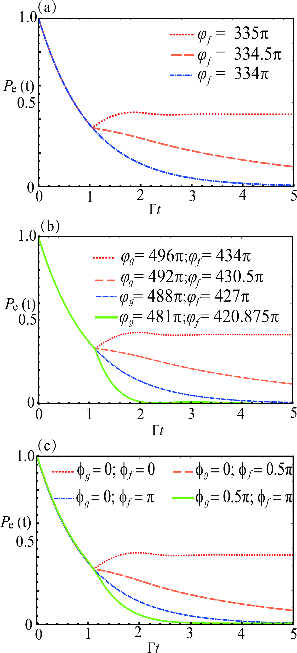
The excitation initially in the 3GA can be carried away by the guided modes. One can adjust the propagating phase through frequency \(\omega _{f}\) in panel (a), the coupling distance \(d\) in panel (b) and the coupling phase differences \(\phi _{\beta },\beta =g,f\) in panel (c) so that a 3GA presents a dynamics exactly the same to a small QE coupled to a waveguide, see the blue dot-dashed lines in Fig. 4. A departure from the exponential decay is visible after time \(t>\tau\). The decay is enhanced (slowed down) comparing to that of a small QE, see the green solid lines (orange dashed lines) in panels (b,c). And it can be found that the parameters for the orange dashed lines is due to the completely suppression of emission via the g-channel, in this context, the dynamics at \(t\geq \tau\) is exactly the same to the 2GA coupled to a waveguide with transition \(\left\vert e\right\rangle \leftrightarrow \left\vert f\right\rangle\), subsequently, the GA is in state \(\left\vert f\right\rangle\) in the long time limit. It is worth pointing out that 1) setting coupling phases \(\phi _{\beta }=(n+1/2)\pi\) make a GA enter an exact Markovian regime irrespectively of any inherent time delay, however, the propagating phases \(\varphi _{\beta }=(n+1/2)\pi\) may result in an exponential decay over time only in the Markovian regime; 2) setting either \(\phi _{f}-\phi _{g}=(2n+1)\pi\) when \(\varphi _{g}=2n\pi +\varphi _{f}\) or \(\phi _{f}-\phi _{g}=2n\pi\) when \(\varphi _{g}=(2n+1)\pi +\varphi _{f}\) also makes a GA show a dynamics exactly the same to a small QE due to the numerator null in Eq.(8 ). A considerable trapping of the probability within the 3GA for long times is clearly visible with a steady value of population, see the red dotted lines. To underly the physics of population trapping, let us find the poles of Eq.(8 ). The pure imaginary poles \(s=-\mathrm{i}\omega\) require\[\begin{eqnarray} \omega &=&\frac{\gamma _{g}}{2}\mathrm{\sin }\left( \varphi _{g}+\omega \tau \right) +\frac{\gamma _{f}}{2}\sin \left( \varphi _{f}+\omega \tau \right) , \\ -\frac{\Gamma }{2} &=&\frac{\gamma _{g}}{2}\cos \left( \varphi _{g}+\omega \tau \right) +\frac{\gamma _{f}}{2}\cos \left( \varphi _{f}+\omega \tau \right) \end{eqnarray}\]to be satisfied. Solving these two equations, the real solution \(\omega =0\) occurs for \(\left\vert g_{1}\right\vert =\left\vert g_{2}\right\vert\) and \(\left\vert g_{3}\right\vert =\left\vert g_{4}\right\vert\) with the four following conditions for phases: \[\label{sec3-08} \begin{eqnarray} \phi _{g} &=&\phi _{f}=2n\pi ;\varphi _{g}=\varphi _{f}=\left( 2n+1\right) \pi ; \\ \phi _{g} &=&\phi _{f}=\left( 2n+1\right) \pi ;\varphi _{g}=\varphi _{f}=2n\pi ; \\ \phi _{g} &=&\varphi _{f}=2n\pi ;\phi _{f}=\varphi _{g}=\left( 2n+1\right) \pi ; \\ \phi _{g} &=&\varphi _{f}=\left( 2n+1\right) \pi ;\phi _{f}=\varphi _{g}=2n\pi . \end{eqnarray}\tag{11}\] As the emission from the excited state to the guided modes are complete suppressed, a dressed atom-photon bound state is formed.

4 Field dynamics↩︎

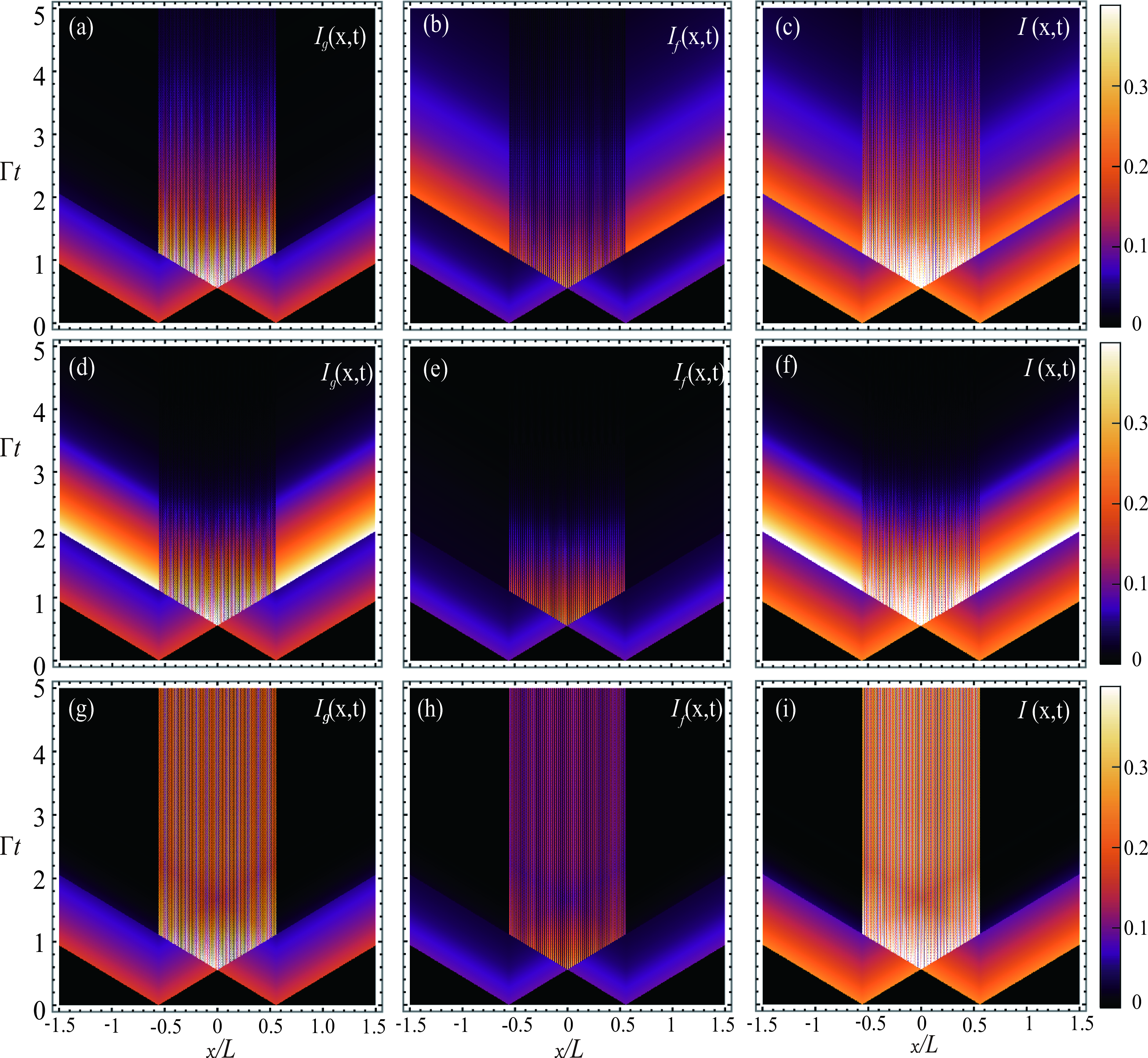
Spontaneous emission from an atom leads to a raise of the photon density in the continuum of the waveguide. To get more physical insight as the radiation field carries information about the atomic dynamics, we consider the local photon density \(I\left( x,t\right) =\left\langle \Psi \left( t\right) \right\vert \hat{a}^{\dagger }\left( x\right) \hat{a}\left( x\right) \left\vert \Psi \left( t\right) \right\rangle\) at position \(x\) and time \(t\), where the real-space field annihilation operator \[\hat{a}\left( x\right) =\int_{0}^{\infty }\frac{d\omega }{\sqrt{2\pi \upsilon _{g}}}\left( e^{-\mathrm{i}\frac{\omega x}{\upsilon _{g}}}\hat{r}_{\omega }+e^{\mathrm{i}\frac{\omega x}{\upsilon _{g}}}\hat{l}_{\omega }\right) \label{sec4-01}\tag{12}\] is the sum of annihilation operators of the right- and left-going modes. Obviously, \(I\left( x,t\right)=I_{g}\left( x,t\right)+I_{f}\left( x,t\right)\) with \(I_{\beta }\left( x,t\right)=\left\vert \Psi _{\beta }\left( x,t\right)\right\vert ^{2}\) due to the presence of the \(g\)- and \(f\)-channel. And the real-space field amplitudes are expressed as\[\label{sec4-02} \begin{align} \Psi_{g}(x,t) &= \frac{1}{\sqrt{2\pi v_{g}}} \int_{0}^{\infty} d\omega \left( e^{-i\frac{\omega x}{v_{g}}}\psi_{gr\omega}\left(t\right) + e^{i\frac{\omega x}{v_{g}}}\psi_{gl\omega}\left(t\right) \right), \\ \Psi_{f}(x,t) &= \frac{1}{\sqrt{2\pi v_{g}}} \int_{0}^{\infty} d\omega \left( e^{-i\frac{\omega x}{v_{g}}}\psi_{fr\omega}\left(t\right) + e^{i\frac{\omega x}{v_{g}}}\psi_{fl\omega}\left(t\right) \right). \end{align}\tag{13}\] With the help of Eq.(4 ) and (8 ), the real-space field amplitudes read \[\label{sec4-03}\begin{align} \Psi_{g}\left( x,t\right) & =-\mathrm{i}\sqrt{\frac{\pi}{2}}\frac{g_{1}}{\upsilon_{g}}u\left( t-\left\vert \tau_{x}^{+}\right\vert \right) \Theta\left( t-\left\vert \tau_{x}^{+}\right\vert \right) \nonumber\\ & -\mathrm{i}\sqrt{\frac{\pi}{2}}\frac{g_{2}}{\upsilon_{g}}u\left( t-\left\vert \tau_{x}^{-}\right\vert \right) \Theta\left( t-\left\vert \tau_{x}^{-}\right\vert \right) \\ \Psi_{f}\left( x,t\right) & =-\mathrm{i}\sqrt{\frac{\pi}{2}}\frac{g_{3}}{\upsilon_{g}}e^{-\mathrm{i}\omega_{f}\left\vert \tau_{x}^{+}\right\vert }u\left( t-\left\vert \tau_{x}^{+}\right\vert \right) \Theta\left( t-\left\vert \tau_{x}^{+}\right\vert \right) \nonumber\\ & -\mathrm{i}\sqrt{\frac{\pi}{2}}\frac{g_{4}}{\upsilon_{g}}e^{-\mathrm{i}\omega_{f}\left\vert \tau_{x}^{-}\right\vert }u\left( t-\left\vert \tau _{x}^{-}\right\vert \right) \Theta\left( t-\left\vert \tau_{x}^{-}\right\vert \right) \nonumber\\ & \null \end{align}\tag{14}\] where \(\tau _{x}^{\pm }=x/\upsilon _{g}\pm \tau /2\). Figure 5 numerically shows the dependence of the photon densities \(I_{g}\left( x,t\right)\), \(I_{f}\left( x,t\right)\) and \(I\left( x,t\right)\) on time and coordinator for \(d\sim L\). After a photon is emitted from the coupling points at \(\pm d/2\), it propagates towards left and right respectively, which is also symbolized by the variables \(t\pm x\) in Eq.(14 ). Some waves propagate back and forth between the regime of the coupling points. The emitted field interferes with itself and produce a series of alternating bright and dark fringes for a period in panels (a-f). During this period, the decay via the \(g/f\)-channel is completely suppressed, see the dark area at \(\left\vert x\right\vert \geq d/2\) in panel (a/e), however, the spontaneous emission still proceeds via the \(f/g\)-channel, see the bright area at \(\left\vert x\right\vert \geq d/2\) in panel (b/d), the decay to \(f/g\)-channel leads the disappearance of the fringes in the long time limit. Therefore, the total density in the waveguide are null in the regime \(\left\vert x\right\vert \leq d/2\) as photons propagate away from the GA, see panels (c) and (f). However, the panels (g-i) in Fig.5 show an stationary interference pattern after an initial rapid change with time, indicating that single photons are spatially localized in a finite regime. This steady state of the field is a localized eigenmode with energy eigenvalue residing directly in the continuum. The localized eigenmode emerges due to the parameters in panels (g-i) satisfying the condition in Eq.(11 ). With the parameters in Eq.(11 ), the real-space field amplitudes in time \(t>\Gamma\) can be further simplified as \[\begin{align} \Psi_{g}\left( x,t\right) & =\frac{\sqrt{2\pi}}{\upsilon_{g}}\frac{g_{1}e^{-\mathrm{i}\omega_{e}t}\sin\left( \omega_{e}\frac{2x+d}{2\upsilon_{g}}\right) }{1+\frac{2\pi\tau}{\upsilon_{g}}\left( \left\vert g_{1}\right\vert ^{2}+\left\vert g_{3}\right\vert ^{2}\right) }\\ \Psi_{f}\left( x,t\right) & =\frac{\sqrt{2\pi}}{\upsilon_{g}}\frac{g_{3}e^{-\mathrm{i}\omega_{e}t}\sin\left[ \left( \omega_{e}-\omega _{f}\right) \frac{2x+d}{2\upsilon_{g}}\right] }{1+\frac{2\pi\tau}{\upsilon_{g}}\left( \left\vert g_{1}\right\vert ^{2}+\left\vert g_{3}\right\vert ^{2}\right) }\end{align}\] As the GA cannot fully decay to the two lower states, thus, less than one photon exits the waveguide on average.

5 Conclusion↩︎

We study the dynamics of an upper level decaying to two lower states by coupling to the guided modes of a linear waveguide in vacuum at two spatially separated points in both Markovian and Non-Markovian regimes. The delay-differential equation for the amplitude of the 3GA in its excited state shows that two transitions induce two different propagating channels for the emitted excitation in the waveguide, which introduces two propagating independent phases \(\varphi _{\beta },\beta =g,f\) on the dynamics of the GA and results in the interference of the atomic population in its excited state after reabsorbing its own emitted excitation at its adjacent coupling point. In the Markovian regime, the \(\Lambda\)-type GA usually decays exponentially, a departure from the exponential decay is presented by a steady value for the dynamics of the GA in the long-time limit. In the non-Markovian regime, the exponential decay is followed by a recurrence of probability when the delay time is much larger than the lifetime of the excited state. However, when \(\tau \approx \Gamma ^{-1}\), its initial exponential decay is followed by an enhanced, slow down of the decay and a complete suppression of the emission of photons into the waveguide. The analysis of the local density of the field shows that the quenching of spontaneous emission is originated from the formation of the dressed atom-photon bound state. We also found that the \(\Lambda\)-type GA can enter the Markovian regime by the interference between two propagating channels in addition to tuning the complex phases of the GA-photon couplings.

References↩︎