¹

1 Introduction↩︎

Nonlinear filtering is a cornerstone of state estimation in dynamic systems, with applications ranging from meteorology to signal processing and geophysical modeling. While the Kalman filter framework is optimal for linear Gaussian systems, it struggles with nonlinearities and non-Gaussian noise, thus requiring approximations. Ensemble Kalman Filters (EnKFs, introduced in [2]) address this challenge by representing the forecast/prior distribution as an ensemble of particles and computing the analysis/posterior distribution in a manner that mimics the Kalman filter update. Here, the terms forecast/prior and analysis/posterior distributions stem from Bayesian analysis and are discussed in [3]. Building on [1], we refer the reader to this work for a comprehensive review of Ensemble Kalman methods. However, the analysis of the EnKF’s accuracy in with repect to the true filtering distribution remains in its infancy. In its regard, [4] recently demonstrated that in a near-linear regime, the distance between the EnKF and the theoretical filtering distribution can be bounded. This suggests that the EnKF may not provide a consistent approximation of the filtering distribution.

Alternative methods, such as Sequential Monte Carlo (SMC), can be designed to be consistent with the underlying nonlinear filtering problem, and do not rely on exactness only for linear Gaussian problems. The monographs [5], [6] provide an overview use of sequential Monte Carlo methods for general discrete time filtering and inference problems, while [7], [8] establish their convergence of sequential Monte Carlo methods, including in specific cases over long time horizons. However, SMC methods suffer from the curse of dimensionality and are currently not directly applicable to high dimensional problems such as those arising in geophysical applications.

In the paper, we focus on a discrete time stochastic filtering problem (i.e. a state estimation problem) where a stochastic dynamical system is observed through linear measurements with noise. Within this relatively restricted setting, we propose an algorithm inspired by SMC particle methods, where Dirac masses are replaced by Gaussian measures. This enables more efficient cover of the state space (potentially mitigating the curse of dimensionality). Our main contributions are as follows: we introduce an algorithm called the ExEnKF (Algorithm [alg:ExEnKF]), prove its asymptotic consistency with the optimal filter (Theorem 1) and demonstrate its robustness to poor initialization and model misspecification (Figure [fig:Trajectories-of-the]) in scenarios where the EnKF fails.

The paper is organized as follows. Section 2 presents the model. Section 3 establishes our convergence result. In Section 4, we introduce a toy model and conduct simulations for a specific set of parameters. Under this setting, we show that the EnKF is insensitive to poor initialization and model misspecification, and performs better than the EnKF.

2 Presentation of the model↩︎

2.1 Notations↩︎

Let \(d\in\mathbb{N}^{*}\). For any \(x\in\mathbb{R}^{d}\), let \(|x|\) denote the Euclidean norm of \(x\). Let \(\mu\) be a probability measure on \(\mathbb{R}^{d}\) (endowed with its Borel \(\sigma\)-algebra) and let \(Q\) be a Markov kernel on \(\mathbb{R}^{d}\). Let \(\phi\,:\,\mathbb{R}^{d}\rightarrow\mathbb{R}\) and \(\psi\,:\,\mathbb{R}^{d}\rightarrow\mathbb{R}^{+*}\) be Borel-measurable functions. We define the following:

• The pushforward measure \(\mu Q\) on \(\mathbb{R}^{d}\): \[\mu Q(dx)=\int_{\mathbb{R}^{d}}\mu(dy)Q(y,dx)\,.\]

• The expectation of \(\phi\) under \(\mu\): \[\langle\mu,\phi\rangle=\int_{\mathbb{R}^{d}}\phi(x)\mu(dx)\,.\]

• The action of \(Q\) on \(\phi\): \[Q\phi(x)=\int_{y\in\mathbb{R}^{d}}Q(x,dy)\phi(y)\,.\]

• The supremum norm of \(\psi\): \[\Vert\psi\Vert_{\infty}=\sup_{x\in\mathbb{R}^{d}}|\psi(x)|\,.\]

• If \(\langle\mu,\psi\rangle>0\), the reweighted measure \(\psi\bullet\mu\): \[\forall f\in\mathcal{M}_{1},\,\psi\bullet\mu(f)=\frac{\mu(f\psi)}{\langle\mu,\psi\rangle}\,,\] where \(\mathcal{M}_{1}\) denotes the set of bounded measurable functions on \(\mathbb{R}^{d}\).

For a symmetric matrix \(M\in\mathbb{R}^{d\times d}\) and vector \(m\in\mathbb{R}^{d}\), let \(\mathcal{N}(m;M)\) denote the Gaussian distribution with mean \(m\) and covariance \(M\). For \(n\in\mathbb{N}^{*}\), let \(I_{n}\) denote the \(n\times n\) identity matrix. Let \(\mathcal{C}(\dots)\) denote the space of continuous functions. A dot (\(\dot{\dots}\)) above a time dependent function (e.g. \(\dot{v}\)) denotes its time-derivative. For any \(n\in\mathbb{N}^{*}\), we define \([n]=\{1,2,\dots,n\}\).

Following [1], [4], we use the Mahalanobis norm \(|u|_{M}^{2}=u^{\top}M^{-1}u\) (for all \(d\in\mathbb{N}^{*}\), for all \(u\in\mathbb{R}^{d}\), \(M\in GL_{d}(\mathbb{R})\)).

2.2 Model.↩︎

Consider a Markov process \((X_{t})_{t\geq0}\) in \(\mathbb{R}^{d_{X}}\) (\(d_{X}\in\mathbb{N}^{*}\)) defined by the recurrence relations \[X_{t}=\Psi(X_{t-1})+V_{t}\,,\label{eq:def-X}\tag{1}\] where

• \(\Psi\,:\,\mathbb{R}^{d_{X}}\rightarrow\mathbb{R}^{d_{X}}\) is a deterministic drift function,

• \((V_{t})_{t\geq1}\) are independent and identically distributed (i.i.d.) centered Gaussian random variables with covariance matrix \(\Sigma\in\mathbb{R}^{d_{X}\times d_{X}}\).

Let \(K\) denote the Markov kernel associated to \((X_{t})_{t\geq0}\).

We observe the process through linear measurements \((Y_{t})_{t\geq1}\in\mathbb{R}^{d_{Y}}\) (\(d_{Y}\in\mathbb{N}^{*}\)), given by: \[Y_{t}=H\times X_{t}+W_{t}\,,\label{eq:def-Y}\tag{2}\] where

• \(H\) in \(\mathbb{R}^{d_{Y}}\times\mathbb{R}^{d_{X}}\) is the observation matrix,

• \((W_{t})_{t\geq1}\) are i.i.d. Gaussian random variables with covariance matrix \(\Gamma\in\mathbb{R}^{d_{Y}\times d_{Y}}\) (independent of \((V_{t})_{t\geq1}\)).

Our goal is to compute the filtering distribution \(\pi_{t}=\mathcal{L}_{\pi_{0}}(X_{t}|Y_{1},\dots,Y_{t})\) for all \(t\geq1\), where the subscript \(\pi_{0}\) means that \(X_{0}\) is distributed according to \(\pi_{0}\). This model is standard and be found in [9], example 3, p. 483.

2.3 Algorithm↩︎

2.3.1 Initialization↩︎

We sample \(N\) independent particles \((X_{0}^{i})_{1\leq i\leq N}\) from the initial distribution \(\pi_{0}\) and approximate \(\pi_{0}\) by the empirical measure: \[\pi_{0}^{N}:=\frac{1}{N}\sum_{k=1}^{N}\delta_{X_{0}^{k}}\,.\]

2.3.2 Propagation step↩︎

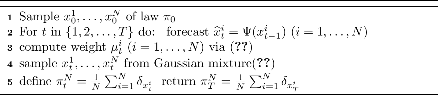
For \(t\geq1\), suppose we have an approximation \(\pi_{t-1}^{N}\) of \(\pi_{t-1}\) \((t\geq1)\): \[\pi_{t-1}^{N}=\frac{1}{N}\sum_{k=1}^{N}\delta_{X_{t-1}^{i}}\] for some particles \(X_{t-1}^{1},\dots,X_{t-1}^{N}\)). Each particle evolves deterministically under \(\Psi\) and generates a Gaussian distribution: \[\forall i\in[N]\,,\,\widehat{\pi}_{t}^{i}=\mathcal{N}(\Psi(X_{t-1}^{i}),\Sigma)\,.\label{eq:ens-gaussiennes}\tag{3}\] We call these Gaussians our forecast ensemble.

2.3.3 Correction step↩︎

We then compute a weight for each Gaussian distribution. \[\mu_{t}^{i}=\int_{\mathbb{R}^{d_{X}}}\frac{\exp(-\frac{1}{2}(u-\Psi(X_{t-1}^{i}))^{\top}\Sigma^{-1}((u-\Psi(X_{t-1}^{i})))\exp(-\frac{1}{2}(Y_{t}-Hu)^{\top}\Gamma^{-1}(Y_{t}-Hu))}{\sqrt{(2\pi)^{d_{X}}\det(\Sigma)}\sqrt{(2\pi)^{d_{Y}}\det(\Gamma)}}du\,.\] We need the following assumption.

We have, for all \(i\), \[\begin{gather} \exp\left(-\frac{1}{2}(u-\Psi(X_{t-1}^{i}))^{\top}\Sigma^{-1}((u-\Psi(X_{t-1}^{i})))\exp(-\frac{1}{2}(Y_{t}-Hu)^{\top}\Gamma^{-1}(Y_{t}-Hu)\right)=\\ \exp\left(-\frac{1}{2}|u-\Psi(X_{t-1}^{i})|_{\Sigma}^{2}-\frac{1}{2}|Y_{t}-Hu|_{\Gamma}^{2}\right)=\\ \text{(we\,write\,\Psi\,for \Psi(X_{t}^{i}))}\\ \exp\left(-\frac{1}{2}|u-(\Sigma^{-1}+H^{\top}\Gamma^{-1}H)^{-1}(\Sigma^{-1}\Psi+H^{T}\Gamma^{-1}Y_{t})|_{(\Sigma^{-1}+H^{\top}\Gamma^{-1}H)^{-1}}^{2}\right.\\ \left.-\frac{1}{2}|\Psi|_{\Sigma}^{2}-\frac{1}{2}|Y_{t}|_{\Gamma}^{2}+\frac{1}{2}|(\Sigma^{-1}\Psi+H^{T}\Gamma^{-1}Y_{t})|_{\Sigma^{-1}+H^{\top}\Gamma^{-1}H}^{2}\right)\,. \end{gather}\] So the weight \[\begin{gather} \mu_{t}^{i}:=\frac{\exp\left(-\frac{1}{2}|\Psi|_{\Sigma}^{2}-\frac{1}{2}|Y_{t}|_{\Gamma}^{2}+\frac{1}{2}|(\Sigma^{-1}\Psi+H^{T}\Gamma^{-1}Y_{t})|_{\Sigma^{-1}+H^{\top}\Gamma^{-1}H}^{2}\right)}{\sqrt{(2\pi)^{d_{X}}\det(\Sigma)}\sqrt{(2\pi)^{d_{Y}}\det(\Gamma)}}\\ \times\sqrt{(2\pi)^{d_{X}}\det((\Sigma^{-1}+H^{\top}\Gamma^{-1}H)^{-1})}\label{eq:weight} \end{gather}\tag{4}\] is explicit.

The forecast ensemble \(\{\widehat{\pi}_{t}^{i}\}_{1\leq i\leq N}\) is updated into a Gaussian mixture: \[\frac{\sum_{i=1}^{N}\mu_{t}^{i}\mathcal{N}((\Sigma^{-1}+H^{\top}\Gamma^{-1}H)^{-1}(\Sigma^{-1}\Psi(X_{t}^{i})+H^{T}\Gamma^{-1}Y_{t});(\Sigma^{-1}+H^{\top}\Gamma^{-1}H)^{-1})}{\sum_{i=1}^{N}\mu_{t}^{i}}\,.\label{eq:gaussian-mixture}\tag{5}\] We then sample N independant points \((X_{t}^{i})_{1\leq i\leq N}\) from this mixture. We call these points our analysis ensemble. From these points, we get an empirical measure we call \[\pi_{t}^{N}=\frac{1}{N}\sum_{i=1}^{N}\delta_{X_{t}^{i}}\,.\]

We refer to this method as the Exact Ensemble Kalman Filter (ExEnKF), as it is asymptotically consistent with the optimal filter (see Theorem 1 below). The pseudocode is provided in [alg:ExEnKF] ³.

3 Mathematical result↩︎

4 Numerical simulations↩︎

In this section, we compare the Exact Ensemble Kalman Filter (ExEnKF) with the standard Ensemble Kalman Filter (EnKF) as described in [1] (Algorithm 2, p. 144). Our experiments are based on variants of the Lorenz-96 model, a widely used benchmark in data assimilation and nonlinear filtering.

4.1 Lorenz-96 Multiscale Model↩︎

Let \(L\), \(J\) in \(\mathbb{N}^{*}\). We have slow variables \(v\in\mathcal{C}(\mathbb{R}^{+},\mathbb{R}^{L})\) and fast variables \(w\in\mathcal{C}(\mathbb{R}^{*},\mathbb{R}^{L\times J})\). Each slow variable \(v_{l}\) is coupled to a group of fast variables \(w_{l}=\{w_{l,j}\}_{j=1}^{J}\). The system is governed by the following ordinary differential equations (ODEs) (the difference between slow and fast variables is purely visual: some oscillate faster than others). For \(l=1,\dots,L\) and \(j=1,\dots,J\): \[\dot{v_{l}}=f_{l}(v)+h_{v}\overline{w}_{l}\,,\,\overline{w}_{l}=\frac{1}{J}\sum_{j=1}^{J}w_{l,j}\,,\label{eq:LMM-01}\tag{6}\] \[\dot{w}_{l,j}=\frac{1}{\epsilon}r_{j}(v_{l},w_{l})\,,\label{eq:LMM-02}\tag{7}\] where \[f_{l}(v)=-v_{l-1}(v_{l-2}-v_{l+1})-v_{l}+F\,,\label{eq:LMM-03}\tag{8}\] \[r_{j}(v_{l},w_{l})=-w_{l,j+1}(w_{l,j+2}-w_{l,j-1})-w_{l,j}+h_{w}v_{l}\,,\label{eq:LMM-04}\tag{9}\] Boundary conditions are imposed as: \[v_{l+L}=v_{l}\,,\,w_{l+L,j}=w_{l,j}\,,\,w_{l,j+J}=w_{l+1},j\,.\label{eq:LMM-05}\tag{10}\] Here:

• \(\epsilon>0\) is a scale separation parameter,

• \(h_{v}\), \(h_{w}\) in \(\mathbb{R}\) govern the couplings between the fast and slow system

• \(F>0\) is a constant forcing.

4.2 Lorenz-96 Singlescale Model↩︎

Let \(v\in\mathcal{C}(\mathbb{R}^{+},\mathbb{R}^{L})\). For \(l=1,\dots,L\), we have ODEs \[\dot{v_{l}}=f_{l}(v)+h_{v}\overline{w}_{l}\,,\,\overline{w}_{l}=M_{l}(v_{l}),\label{eq:LSM-01}\tag{11}\] where \(f_{l}\) is defined in (8 ), and \((M_{l})_{1\leq l\leq L}\) are suitably chosen functions.

We follow here the reasoning of [1], p. 146. If \(\epsilon\ll1\), the dynamics for the \(w\) governed by (7 ) evolve on a much faster timescale than the dynamics for the \(v\) governed by (6 ). Thus it is a reasonable approximation to think of \(v\) as frozen in (7 ). If we assume that the dynamics of \(w\) with \(v\) frozen are ergodic with invariant measure \(\mu^{v}(dw)\) (a measure in \(w\), parametrized by \(v\)) then the averaging principle ([13]–[15]) suggests that we may make the approximation (in (6 )) \[\overline{w}\approx M(v):=\int\left(\frac{1}{J}\sum_{j=1}^{J}w_{j}\right)\mu^{v}(dw)\,.\] We call \(M_{l}\) the \(l\)-th component of \(M\) above. We can add the approximation that, for all \(l\), \(M_{l}(v)\) is a function \(m(v_{l})\) of the sole component \(v_{l}\) (and not of the whole vector \(v\)) (approximation that is shown to be valid for large \(J\) in [16]), then we arrive at the singlescale Lorenz-96 model (11 ). The function \(m\) is not given explicitly, but may be estimated from data. Figure 2.1 of [1] shows such an \(m\) fit using Gaussian process regression methodology. Essentially, you need to make a simulation of \((v,w)\) solution of (6 )-(7 ) then fit a function \(m\) such that \[\frac{1}{J}\sum_{j=1}^{J}w_{l,j}=m(v_{l})\,,\,\forall l\,.\]

4.3 Numerical experiments↩︎

We wish to compare our algorithm to the EnKF of [1] (the code is available at https://github.com/EdoardoCalvello/EnsembleKalmanMethods/).

4.3.1 Generating the true signal↩︎

To create a benchmark dataset, we simulate the true signal using the Lorenz-96 multiscale model. We introduce a positive \(\tau\) (\(\tau\) will be the observation time interval). Let \(L=9\), \(J=8\). We initialize the system with arbitrary values for \((v_{0},w_{0})=:x_{0}^{\dagger}\in\mathbb{R}^{L}\times\mathbb{R}^{L\times J}\) (all the components set to zero). For \(t=0,1,2,\dots,T_{\max}-1\) (\(T_{max}\in\mathbb{N}\)), we proceed as follows

• Simulate the Lorenz-96 dynamics over a time interval of length \(\tau\) starting from \(x_{t}^{\dagger}\) yielding a vector \(\varphi(x_{t}^{\dagger})\).

• Update the true signal \[x_{t+1}^{\dagger}=\varphi(x_{t}^{\dagger})+\sigma Z_{t+1}\] (where \(Z_{t+1}\sim\mathcal{N}(0,I_{L+J})\) is independent of \(Z_{1},\dots,Z_{t}\) and \(\sigma>0\). As in [1], [4], the superscript \(\dagger\) indicate that \(x_{t}^{\dagger}\) is the true signal, and remain fixed throughout the experiment.

4.3.2 Generating the true observations↩︎

We define the observation operator \(H\in\mathbb{R}^{9\times6}\) as \[H=\left[\begin{array}{ccccccccc} 1 & 0 & 0 & 0 & 0 & 0 & 0 & 0 & 0\\ 0 & 1 & 0 & 0 & 0 & 0 & 0 & 0 & 0\\ 0 & 0 & 0 & 1 & 0 & 0 & 0 & 0 & 0\\ 0 & 0 & 0 & 0 & 1 & 0 & 0 & 0 & 0\\ 0 & 0 & 0 & 0 & 0 & 0 & 1 & 0 & 0\\ 0 & 0 & 0 & 0 & 0 & 0 & 0 & 1 & 0 \end{array}\right]\,.\] For \((x_{1},x_{2},\dots,x_{9})^{T}\in\mathbb{R}^{L}\), the observation is \[Hx^{T}=(x_{1},x_{2},x_{4},x_{5},x_{7},x_{8})^{T}\,.\] The true observations \(y_{t}^{\dagger}\) are generated as: \[y_{t}^{\dagger}=H\overline{x}_{t}^{\dagger}+\gamma\eta_{t}\,,\label{eq:true-observations}\tag{12}\] where

• \(\overline{x}_{t}^{\dagger}\) is the \(L\) first components of \(x_{t}^{\dagger}\) (the slow variables \(v\)),

• \(\eta_{t}\sim\mathcal{N}(0,I_{6})\) are independent standard Gaussian random variables,

• \(\gamma>0\) controls the observation noise.

As in [1], [4], the superscript \(\dagger\) indicates that \(y_{t}^{\dagger}\) is the true observations and remain fixed throughout the experiment.

4.3.3 Running ExEnKF↩︎

We apply Algorithm [alg:ExEnKF] (ExEnKF) to the observations \((y_{t}^{\dagger})_{t\geq1}\). To do so, we use the function \(m\) estimated in [1]. For an initial condition \(v_{0}\in\mathbb{R}^{L}\), we define \(\Psi(v_{0})\) as the solution of the singlescale Lorenz-96 model (11 ) at time \(\tau\), with \(M_{l}=m\) for all \(l\). We then run Algorithm [alg:ExEnKF] (loop \(T_{\text{max}}\) times) with:

• the dynamics \(\Psi=\varphi\),

• the observations \((y_{t}^{\dagger})_{t\geq1}\),

• a fixed number of particles \(N\).

This yields empirical measures \((\pi_{t}^{N})_{1\leq t\leq T_{\max}}\).

4.3.4 Model misspecification and poor initialization↩︎

To test the robustness of ExEnKF, we intentionally introduce two challenges:

1. Model misspecification: The observations \((y_{t}^{\dagger})_{t\geq1}\) are generated using the multiscale Lorenz-96 model, but ExEnKF assumes the singlescale model for state estimation.

2. Poor initialization: The particles in ExEnKF are initialized with \(x_{0}^{i}\sim\mathcal{N}(10,10\times I_{L})\), rather than the true initial condition \(x_{0}^{\dagger}=0\).

For each time \(t\), we compute the empirical mean \(\langle\pi_{t}^{N},\phi_{3}\rangle\) where \(\phi_{3}\) is defined by \(\phi(x_{1},\dots,x_{9})=x_{3}\) (the third component of the state). This allows us to compare the estimated trajectory of the hidden component \(x_{3}\) with the true signal \(\phi_{3}(x_{t}^{\dagger})\). Note that the third component of \(x_{t}^{\dagger}\) does not appear in the observations \(y_{t}^{\dagger}\) (see \(H\) above), making this a stringent test of the algorithm’s ability to track unobserved components.

4.3.5 Results↩︎

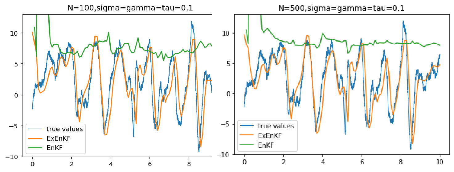
We present the results in Figure [fig:Trajectories-of-the] which shows the true trajectory (blue) alongside the estimates from EnKF (green) and ExEnKF (orange). In all experiments, we set \[\sigma=\gamma=\tau=0.1.\] These parameters correspond to a highly stochastic regime, where traditional EnKF methods often struggle. As shown in Figure 2.5 of [4], EnKF performs well for \(\sigma=\gamma=0.1\) and \(\tau=10^{-3}\). EnKF’s principle is that you run computations similar to those used for a Kalman filter (where all the measures are Gaussian and \(\Psi\) is a linear operator). When \(\tau\) increases, this approximation is bound to fail (see Figure [fig:Trajectories-of-the]). We also see in Figure [fig:Trajectories-of-the] that ExEnKF manages to track down the true trajectory after a poor initialization at time \(0\). We tried the various algorithms with \(N=100\) and \(N=500\) without noticeable variation.

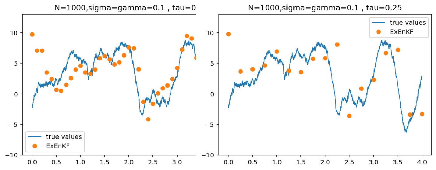
Like in [4], the algorithm struggles to recover the original trajectory when \(\tau\) increases (see Figure [fig:Trajectories-of-the-1]).

References↩︎