Closed-form solutions to some generalized variational inference problems
June 24, 2026
Abstract
The Donsker–Varadhan formula characterizes the ordinary Bayesian posterior as the solution of an unrestricted \(\mathsf{KL}\)-regularized variational problem. Generalized variational inference replaces this regularizer by other divergences, but the resulting measure-valued optimization problem is often studied only after restriction to a parametric variational family. This paper studies the unrestricted measure-level problem. Given a measurable space \((\mathcal{Z},\mathfrak{Z})\), a prior probability measure \(P\), a measurable loss \(\ell:\mathcal{Z}\to(-\infty,\infty]\), a regularization strength \(\alpha>0\), and a divergence \(\mathsf{D}(Q\Vert P)\), we seek probability measures in \[\underset{Q\in\mathcal{P}(\mathcal{Z})}{\mathrm{arg\,min}}\left\{\int_{\mathcal{Z}} \ell\,\mathrm{d}Q+\alpha\mathsf{D}(Q\Vert P)\right\}.\] For \(f\)-divergence penalties we derive a scalar inverse-gradient density formula and a one-dimensional dual identity; the Kullback–Leibler, Cressie–Read, and squared-Hellinger problems are treated as examples. Reverse \(f\)-divergences and mixed forward/reverse Kullback–Leibler penalties follow from the same separable integral principle. For Bregman divergences between densities we obtain a density-space solution with a scalar mass multiplier, including least-squares, density-power, and Burg/Itakura–Saito examples. For Rényi penalties of order \(r>1\) we derive a normalized truncated-power characterization and a threshold equation for every global optimizer. Finite model-weight formulas and simple conjugate Bayesian model illustrations show how these closed forms are realized in practice and differ from the traditional solutions.
generalized variational inference; \(f\)-divergence; Bregman divergence; Rényi divergence; Gibbs posterior; Donsker–Varadhan formula
1 Introduction↩︎
Classical Bayesian inference is concerned with the posterior probability measure \[Q(A\mid x)= \frac{\int_A L(x\mid\theta)\,P(\mathrm{d}\theta)}{\int_\Theta L(x\mid\vartheta)\,P(\mathrm{d}\vartheta)}, \qquad A\in\mathfrak{T},\] where \((\Theta,\mathfrak{T})\) is a measurable parameter space, \(P\) is the prior probability measure, \(x\) is the observed datum, and \(L(x\mid\theta)\) is the likelihood of \(x\) under the parameter value \(\theta\). When there are several observations, \(x\) may denote a sample; i.e., \(x=(y_1,\ldots,y_N)\). If \(\ell(\theta)=-\log L(x\mid\theta)\) up to an additive constant independent of \(\theta\), then this posterior measure is equivalently the solution of \[\underset{Q\in\mathcal{P}(\Theta)}{\mathrm{arg\,min}} \left\{\int_\Theta \ell\,\mathrm{d}Q+\mathsf{KL}(Q\Vert P)\right\}.\] This is an instance of the Gibbs/Donsker–Varadhan variational formula [1], and it is one of the bridges between Bayesian inference, convex duality, and statistical learning.
Let \((\mathcal{Z},\mathfrak{Z})\) be a measurable space and let \(P\in\mathcal{P}(\mathcal{Z})\) be a prior probability measure. For a measurable loss \(\ell:\mathcal{Z}\to(-\infty,\infty]\), a divergence \(\mathsf{D}\), and \(\alpha>0\), the generalized variational inference (GVI) problem considered here has the following possibly empty or non-singleton solution set \[\label{eq:master-intro} \underset{Q\in\mathcal{P}(\mathcal{Z})}{\mathrm{arg\,min}} \left\{\int_{\mathcal{Z}}\ell\,\mathrm{d}Q+\alpha\mathsf{D}(Q\Vert P)\right\}.\tag{1}\] In generalized Bayes, \(\ell\) may be any loss connecting the parameter to the data. When \(\mathsf{D}(Q\Vert P)=\mathsf{KL}(Q\Vert P)\), the solution satisfies \(\mathrm{d}Q^\star/\mathrm{d}P\propto \exp(-\ell/\alpha)\). The parameter \(\alpha\) therefore plays the role of a temperature: increasing \(\alpha\) weakens the loss tilt and keeps the solution closer to the prior, while decreasing \(\alpha\) concentrates more strongly near small-loss states.
The aim of this paper is to identify classes of divergences for which 1 has an exact density-form solution. We prove three main results. First, for differentiable strictly convex \(f\)-divergences, the solution is obtained by applying the inverse derivative of \(f\) to a shifted and rescaled loss, followed by one scalar normalization. Secondly, for separable Bregman divergences between densities, the solution is a mirror-descent step in density space, again with one scalar mass multiplier. Here separable means that, after fixing a dominating measure, the divergence is the integral of a pointwise function of the candidate density and the prior density, as in the Bregman-distance class studied by [2]. Thirdly, for the logarithmic \(\mathcal{L}^r(P)\) form of the Rényi divergence with \(r>1\), every global optimizer has a normalized positive-part power-law form. These formulas make exact GVI solutions available as mathematical objects in their own right, rather than only as targets for approximate variational optimization.
The relevant variational identities have a substantial history. \(\mathsf{KL}\)-regularized solutions appear in minimization views of Bayesian inference and loss-based Bayes [3], [4]. \(\mathsf{KL}\)-regularized estimators also underlie information-theoretic and PAC-Bayes bounds [5], [6]. The optimization-centric formulation of Bayesian and generalized variational inference was developed systematically by [7]; see also the machine-learning exposition of [8]. In contrast with works that primarily study computational restrictions or variational families, including GVI and related variational inference methods [7], [8], the present paper keeps the feasible set equal to the full space of probability measures.
For \(f\)-divergences, foundational sources include [9] and [10], with modern variational forms appearing in divergence estimation and learning [11]–[14]. The closest antecedent for the \(f\)-divergence part is the generalized Gibbs formula of [15]. If \(f^*\) denotes the Fenchel conjugate, then under the hypotheses of [15] one has \[\Lambda_f^P[g] = \inf_{\nu\in\mathbb{R}}\left\{\nu+\int_{\mathcal{Z}} f^*(g-\nu)\,\mathrm{d}P\right\} = \sup_Q\left\{\int_{\mathcal{Z}}g\,\mathrm{d}Q-\mathsf{D}_f(Q\Vert P)\right\}.\] When the infimum is attained at \(\nu^\star\) and \(f^*\) is differentiable, the optimizing measure has density \((f^*)'(g-\nu^\star)\), where \((f^*)'\) denotes the derivative of the scalar convex conjugate \(f^*\). Under strict convexity and differentiability, this derivative is the inverse-gradient map \((f')^{-1}\) on the relevant range. Our \(f\)-divergence theorem is the loss-minimization version of this identity with \(g=-\ell/\alpha\), together with explicit solution expressions.
Bregman divergences originate in the projection method of [16] and are closely tied to Legendre-function Bregman projections [17], mirror descent [18], and convex integral minimization under linear constraints [19]–[21]; see also [2] for generalized projections of non-negative functions using both \(f\)-divergence and Bregman-type distances. Finite-dimensional analogues include sparsemax and entmax maps, which are regularized simplex prediction maps induced by Euclidean or Tsallis-type penalties [22], [23].
Rényi divergences originate with [24] and have their own Donsker–Varadhan-type variational theory [25]–[27]. These works characterize or estimate Rényi divergences. The problem studied here is different: a linear expected loss plus a logarithmic \(\mathcal{L}^r(P)\) penalty over \(\mathrm{d}Q/\mathrm{d}P\). The resulting optimizer is not exponential but a positive-part power law with a threshold equation.
Two examples make the formulas concrete. First, a finite model list turns the measure-level problem into explicit generalized posterior model weights, recovering ordinary Bayesian model averaging in the \(\mathsf{KL}\) case. Secondly, two conjugate models illustrate the density shapes produced by the different divergence regularizers.
1.0.0.1 Contributions.
We provide exact solutions for four classes of examples: \(f\)-divergences, including \(\mathsf{KL}\), Cressie–Read cases such as Pearson \(\chi^2\), reverse \(f\)-divergence, reverse \(\mathsf{KL}\), and mixed-direction \(\mathsf{KL}\) cases; separable Bregman divergences, including least-squares, density-power, and Burg/Itakura–Saito cases; Rényi regularization with \(r>1\); and finite model-weight examples together with density-shape illustrations in standard conjugate models. All results are stated for general measurable spaces, except the Bregman section, which fixes a dominating measure for the two densities. Complete proofs of all results appear in the supplementary material.
2 Technical preliminaries↩︎
2.1 Notation and standing assumptions↩︎
Condition 1 (Measurable-space hypothesis). Let \((\mathcal{Z},\mathfrak{Z})\) be a measurable space and let \(P\in\mathcal{P}(\mathcal{Z})\) be fixed. The loss \(\ell:\mathcal{Z}\to(-\infty,\infty]\) is measurable, belongs to \(\mathcal{L}^1(P)\), and is bounded below \(P\)-almost surely.
For two probability measures \(Q\) and \(P\) on \((\mathcal{Z},\mathfrak{Z})\), the notation \(Q\ll P\) means that \(P(A)=0\) implies \(Q(A)=0\) for every \(A\in\mathfrak{Z}\). In this case \(u=\mathrm{d}Q/\mathrm{d}P\) denotes the Radon–Nikodym derivative, so \(\int_{\mathcal{Z}}\ell\,\mathrm{d}Q=\int_{\mathcal{Z}}\ell u\,\mathrm{d}P\) and \(\int_{\mathcal{Z}}u\,\mathrm{d}P=1\). We write \(a_+=\max\{a,0\}\). An integral of a measurable function is allowed to take the value \(+\infty\); it is interpreted as an extended integral in \((-\infty,\infty]\) whenever the negative part is finite. Boundedness below is enough to make \(\int_{\mathcal{Z}}\ell\,\mathrm{d}Q\) an extended real number with finite negative part for every \(Q\ll P\), and it also makes the \(\mathsf{KL}\) normalizer finite. The additional assumption \(\ell\in\mathcal{L}^1(P)\) is a simplifying nondegeneracy condition ensuring that the objective is finite at the reference measure \(Q=P\). Several results can be stated under weaker hypotheses, but Condition 1 keeps the exposition uniform.
A function \(g:\mathbb{R}\to(-\infty,\infty]\) is proper if it is not identically \(\infty\). It is lower semicontinuous (LSC) if all sets \(\{t:g(t)\le c\}\) are closed. Its Fenchel conjugate is \(g^*(y)=\sup_{t\in\mathbb{R}}\{ty-g(t)\}\), \(y\in\mathbb{R}\). For a proper convex function \(g\), a real number \(y\) is a subgradient of \(g\) at \(t\) if \(g(s)\ge g(t)+y(s-t)\) for every \(s\in\mathbb{R}\); the set of all such subgradients is denoted by \(\partial g(t)\). We use the Fenchel–Young inequality \(g(t)+g^*(y)\ge ty\), with equality if and only if \(y\in\partial g(t)\); compare Lemma 1. These are standard facts of convex optimization; see, for example, [21]. For the affine mass constraint \(\int_{\mathcal{Z}}u\,\mathrm{d}P=1\), the corresponding Lagrange multiplier is represented by a constant \(\lambda\), since \(\lambda\int_{\mathcal{Z}}(v-u)\,\mathrm{d}P=0\) for all feasible \(u\) and \(v\). The scalar monotonicity fact used to identify such multipliers is stated as Lemma 4 in the supplementary material.
3 \(f\)-divergence regularization↩︎
3.1 General solution↩︎
Let \(f:[0,\infty)\to(-\infty,\infty]\) be proper, LSC, convex, finite and differentiable on \((0,\infty)\), and satisfy \(f(1)=0\) and \(f(t)\ge0\), with equality only at \(t=1\). Extend \(f(t)=\infty\) for \(t<0\) and define \[\label{eq:fdiv-def} \mathsf{D}_f(Q\Vert P)= \begin{cases} \displaystyle \int_{\mathcal{Z}} f\!\left(\frac{\mathrm{d} Q}{\mathrm{d} P}\right)\,\mathrm{d}P, & Q\ll P,\\[0.5em] \infty, & \text{otherwise.} \end{cases}\tag{2}\] Under this convention, any probability measure \(Q\) that is not absolutely continuous with respect to \(P\) has infinite divergence. It is the usual convention for the examples in this paper; more general conventions for singular parts are discussed by [28] and [15]. With \(u=\mathrm{d}Q/\mathrm{d}P\), the optimization problem is \[\label{eq:f-primal} \inf_{u\in\mathcal{U}}\int_{\mathcal{Z}}\{\ell u+\alpha f(u)\}\,\mathrm{d}P, \qquad \mathcal{U}=\left\{u:\mathcal{Z}\to[0,\infty)\text{ measurable}:\int_{\mathcal{Z}}u\,\mathrm{d}P=1\right\}.\tag{3}\] For the explicit inverse-gradient formula we assume, in addition, that \(f\) is strictly convex on \((0,\infty)\), \(f'_+(0)=\lim_{t\downarrow0}f'(t)\in[-\infty,\infty)\), and \(f'_-(\infty)=\lim_{t\uparrow\infty}f'(t)=\infty\).
Theorem 1 (\(f\)-divergence solution). Assume Condition 1 and the hypotheses on \(f\) stated in this subsection. For \(\lambda\in\mathbb{R}\) define \[\label{eq:u-lambda-main} u_\lambda(z)=\underset{t\ge0}{\mathrm{arg\,min}}\{\alpha f(t)+(\ell(z)+\lambda)t\}.\tag{4}\] Then \(u_\lambda\) is measurable and is given by \[\label{eq:u-inverse-main} u_\lambda(z)= \begin{cases} 0, & -\dfrac{\ell(z)+\lambda}{\alpha}\le f'_+(0),\\[0.8em] (f')^{-1}\!\left(-\dfrac{\ell(z)+\lambda}{\alpha}\right), & -\dfrac{\ell(z)+\lambda}{\alpha}> f'_+(0), \end{cases}\tag{5}\] with the convention that the first branch is void when \(f'_+(0)=-\infty\). There is a unique \(\lambda^\star\in\mathbb{R}\) satisfying \[\label{eq:f-normalization-main} \int_{\mathcal{Z}}u_{\lambda^\star}\,\mathrm{d}P=1.\tag{6}\] The unique minimizer of 3 is \(u^\star=u_{\lambda^\star}\); equivalently, the solution of 1 with \(\mathsf{D}=\mathsf{D}_f\) is the probability measure \(Q^\star\) satisfying \(\mathrm{d}Q^\star/\mathrm{d}P=u_{\lambda^\star}\).
Proof. See Supplement 10. ◻
Corollary 1 (\(f\)-divergence dual identity). Under the hypotheses of Theorem 1, \[\label{eq:f-dual-main} \inf_{u\in\mathcal{U}}\int_{\mathcal{Z}}\{\ell u+\alpha f(u)\}\,\mathrm{d}P =\sup_{\lambda\in\mathbb{R}}\left\{-\lambda-\alpha\int_{\mathcal{Z}} f^*\!\left(-\frac{\ell+\lambda}{\alpha}\right)\,\mathrm{d}P\right\}.\tag{7}\] The supremum is attained at the normalizing multiplier \(\lambda^\star\) from Theorem 1.
Proof. See Supplement 10. ◻
3.2 Examples↩︎
3.2.0.1 Kullback–Leibler divergence.
For \(f(t)=t\log t-t+1\), \(f'(t)=\log t\). Since \(\ell\) is bounded below, \(Z_\alpha=\int_{\mathcal{Z}}\exp(-\ell/\alpha)\,\mathrm{d}P<\infty\), and \[\label{eq:kl-main} \frac{\mathrm{d}Q^\star}{\mathrm{d}P}(z)=\frac{\exp(-\ell(z)/\alpha)}{Z_\alpha}.\tag{8}\] The optimal value is \(-\alpha\log Z_\alpha\), recovering the Gibbs/Donsker–Varadhan formula.
3.2.0.2 Cressie–Read power divergences and Pearson \(\chi^2\).
For \(\gamma\in\mathbb{R}\setminus\{0,1\}\), the Cressie–Read family may be written, up to the usual normalization convention, as \[f_\gamma(t)=\frac{t^\gamma-\gamma t+\gamma-1}{\gamma(\gamma-1)}, \qquad t>0.\] The limiting cases \(\gamma\to1\) and \(\gamma\to0\) give forward and reverse Kullback–Leibler divergences, and particular choices give the Pearson \(\chi^2\), modified \(\chi^2\), and Hellinger cases; see [29] and [11]. For \(\gamma>1\), the inverse-gradient formula gives \[u_\lambda(z)= \left(1-\frac{(\gamma-1)(\ell(z)+\lambda)}{\alpha}\right)_+^{1/(\gamma-1)}, \qquad \int_{\mathcal{Z}}u_{\lambda^\star}\,\mathrm{d}P=1,\] with the unique normalizing multiplier. The unscaled Pearson generator used here is \(f(t)=(t-1)^2\), equal to \(2f_2(t)\) in the preceding convention, and therefore \[\label{eq:chi-main} u_\lambda(z)=\left(1-\frac{\ell(z)+\lambda}{2\alpha}\right)_+, \qquad \int_{\mathcal{Z}} u_{\lambda^\star}\,\mathrm{d}P=1.\tag{9}\] Thus \(Q^\star\) is a clipped affine reweighting of \(P\). This finite-dimensional form is the same thresholding mechanism that appears in distributionally robust optimization (DRO) with \(f\)-divergence balls [30].
3.2.0.3 Reverse \(f\)-divergences.
Reverse \(f\)-divergence regularization is also separable after a change of generator. Let \(r=\mathrm{d}Q/\mathrm{d}P\) and assume \(Q\ll P\) and \(P\ll Q\). Then \[\label{eq:perspective-main} \mathsf{D}_f(P\Vert Q)=\int_{\mathcal{Z}} f^\diamond(r)\,\mathrm{d}P, \qquad f^\diamond(r)=r f(1/r),\quad r>0.\tag{10}\] The map \(f^\diamond\) is the one-dimensional perspective transform of \(f\) and is convex; the convexity of perspective functions is a standard fact of convex analysis [21]. If \(f^\diamond\) is strictly convex and differentiable and the corresponding scalar minimizer can be normalized, any minimizer of \[\underset{Q:Q\ll P,\,P\ll Q}{\mathrm{arg\,min}}\left\{\int_{\mathcal{Z}}\ell\,\mathrm{d}Q+\alpha \mathsf{D}_f(P\Vert Q)\right\}\] has likelihood ratio \[\label{eq:reverse-f-main} r^\star(z)=\left((f^\diamond)'\right)^{-1}\!\left(-\frac{\ell(z)+\lambda^\star}{\alpha}\right), \qquad \int_{\mathcal{Z}} r^\star\,\mathrm{d}P=1.\tag{11}\] For reverse \(\mathsf{KL}\), \(f(t)=t\log t-t+1\) gives \(f^\diamond(r)=-\log r+r-1\). For any normalizing multiplier with \(\alpha+\ell+\lambda^\star>0\) \(P\)-a.s., \[\label{eq:reverse-kl-main} r^\star(z)=\frac{\alpha}{\alpha+\ell(z)+\lambda^\star}.\tag{12}\]
3.2.0.4 Mixed-direction \(\mathsf{KL}\).
For a mixed penalty \(a\mathsf{KL}(Q\Vert P)+b\mathsf{KL}(P\Vert Q)\) with \(a,b>0\), the effective generator is \[f_{a,b}(r)=a(r\log r-r+1)+b(-\log r+r-1), \qquad f'_{a,b}(r)=a\log r+b(1-1/r).\] Inverting \(f'_{a,b}\) gives a closed form in the principal branch of the Lambert \(W\) function. Here \(\mathrm{W}\) denotes the principal real branch of the inverse of \(w\mapsto w e^w\) on \([0,\infty)\) [31]: \[\label{eq:mixed-kl-main} r_\lambda(z)=\frac{b/a}{\mathrm{W}\!\left((b/a)\exp\left[b/a+\frac{\ell(z)+\lambda}{\alpha a}\right]\right)}, \qquad \int_{\mathcal{Z}} r_{\lambda^\star}\,\mathrm{d}P=1.\tag{13}\] For \(a=b=1\) the penalty is the Jeffreys divergence [32], \[\mathsf{J}(Q,P)=\mathsf{KL}(Q\Vert P)+\mathsf{KL}(P\Vert Q),\] and 13 gives its closed-form likelihood ratio. The derivations are given in Supplement 12.
3.3 Squared-Hellinger divergence↩︎
For \(f(t)=(\sqrt t-1)^2\), the derivative \(f'(t)=1-t^{-1/2}\) has finite limit \(f'_-(\infty)=1\). Thus Theorem 1 does not apply, because the scalar objective may fail to be coercive unless the shifted loss is sufficiently positive. Suppose there is \(\lambda^\star\) such that \(\alpha+\ell+\lambda^\star>0\) \(P\)-a.s. and \[\int_{\mathcal{Z}}\left(\frac{\alpha}{\alpha+\ell+\lambda^\star}\right)^2\,\mathrm{d}P=1.\] Then the unique minimizer is \[\label{eq:hell-main} \frac{\mathrm{d}Q^\star}{\mathrm{d}P}(z)=\left(\frac{\alpha}{\alpha+\ell(z)+\lambda^\star}\right)^2.\tag{14}\] The positivity condition is not vacuous: if \(\alpha+\ell(z)+\lambda\le0\) on a set of positive \(P\)-mass, the pointwise scalar objective is not bounded below along large values of the density on that set. The derivation is given in Supplement 11.
4 Bregman divergence regularization↩︎
4.1 General solution↩︎
Condition 2 (Dominating measure for Bregman divergences). Let \(\mu\) be a \(\sigma\)-finite measure on \((\mathcal{Z},\mathfrak{Z})\). Assume \(P\ll\mu\) with density \(p=\mathrm{d}P/\mathrm{d}\mu\), and consider candidates \(Q\ll\mu\) with density \(q=\mathrm{d}Q/\mathrm{d}\mu\). Assume that \(\ell\) is finite and bounded below \(\mu\)-almost surely.
Let \(I\) be either \([0,\infty)\) or \((0,\infty)\). Let \(\psi:I\to(-\infty,\infty]\) be proper, LSC, strictly convex, and differentiable on \((0,\infty)\). Assume \(\psi'_-(\infty)=\infty\). If \(I=(0,\infty)\), assume also \(p>0\) \(\mu\)-a.e. and \(\psi'_+(0)=-\infty\); this is the barrier-domain case. If \(I=[0,\infty)\), assume \(\psi'_+(0)>-\infty\), put \(\psi'_+(0)=\lim_{t\downarrow0}\psi'(t)\), and interpret \(\psi'(p)\) as \(\psi'_+(0)\) on the set where \(p=0\). Define \[\label{eq:breg-def-main} \mathsf{D}_\psi(Q\Vert P)=\int_{\mathcal{Z}}\{\psi(q)-\psi(p)-\psi'(p)(q-p)\}\,\mathrm{d}\mu.\tag{15}\] Keeping only the pointwise terms in the objective that depend on \(q\) gives the reduced problem \[\label{eq:breg-primal-main} \inf_{q:\int_{\mathcal{Z}} q\,\mathrm{d}\mu=1}\int_{\mathcal{Z}}\{\alpha\psi(q)+(\ell-\alpha\psi'(p))q\}\,\mathrm{d}\mu,\tag{16}\] with \(q(z)\in I\) \(\mu\)-a.e. This reduced formulation is obtained from 15 by omitting pointwise terms that do not depend on \(q\). Indeed, expanding 15 in the original objective gives 16 plus the constant \(\alpha\int_{\mathcal{Z}}\{\psi'(p)p-\psi(p)\}\,\mathrm{d}\mu\), which is independent of the candidate density \(q\). When this constant is finite, adding or removing it leaves the set of minimizers unchanged. The proof again uses the scalar Lagrange multiplier for the mass constraint and pointwise minimization of the separable integrand.
Theorem 2 (Bregman density solution). Assume Conditions 1 and 2, and the hypotheses on \(I\) and \(\psi\), above. For \(\lambda\in\mathbb{R}\) define \[\label{eq:q-lambda-main} q_\lambda(z)=\underset{t\in I}{\mathrm{arg\,min}}\{\alpha\psi(t)+(\ell(z)-\alpha\psi'(p(z))+\lambda)t\}.\tag{17}\] Then \(q_\lambda\) is measurable. If \(\lambda^\star\) satisfies \(\int_{\mathcal{Z}} q_{\lambda^\star}\,\mathrm{d}\mu=1\) and the reduced objective in 16 is finite at \(q_{\lambda^\star}\), then \(q^\star=q_{\lambda^\star}\) is the unique minimizer of 16 . At points \(z\) for which the scalar minimizer in 17 lies in the open interval \((0,\infty)\), \[\label{eq:breg-inverse-main} q_\lambda(z)=(\psi')^{-1}\!\left(\psi'(p(z))-\frac{\ell(z)+\lambda}{\alpha}\right).\tag{18}\] If \(I=[0,\infty)\), this is clipped at zero: \[\label{eq:breg-clip-main} q_\lambda(z)= \begin{cases} 0, & \psi'(p(z))-\dfrac{\ell(z)+\lambda}{\alpha}\le\psi'_+(0),\\[0.8em] (\psi')^{-1}\!\left(\psi'(p(z))-\dfrac{\ell(z)+\lambda}{\alpha}\right),&\text{otherwise.} \end{cases}\tag{19}\] If the constant \(\alpha\int_{\mathcal{Z}}\{\psi'(p)p-\psi(p)\}\,\mathrm{d}\mu\) is finite, then the probability measure with density \(q^\star\) is also the unique minimizer of the original Bregman-regularized objective.
Proof. See Supplement 13. ◻
Corollary 2 (Bregman normalizer). Under the hypotheses of Theorem 2, suppose \[G(\lambda)=\int_{\mathcal{Z}}q_\lambda\,\mathrm{d}\mu<\infty \quad\text{for all }\lambda\in\mathbb{R},\qquad \lim_{\lambda\to\infty}G(\lambda)=0,\qquad \lim_{\lambda\to-\infty}G(\lambda)=\infty.\] Then there is a unique \(\lambda^\star\) with \(G(\lambda^\star)=1\). If the reduced objective is finite at \(q_{\lambda^\star}\), then Theorem 2 applies.
Corollary 3 (Bregman dual identity). Under the hypotheses of Theorem 2, suppose that \(\lambda^\star\) satisfies \(\int_{\mathcal{Z}}q_{\lambda^\star}\,\mathrm{d}\mu=1\) and that the reduced objective is finite at \(q_{\lambda^\star}\). Let \(\psi^*\) denote the Fenchel conjugate of \(\psi\) after extending \(\psi\) by \(\infty\) outside \(I\). Then \[\label{eq:breg-dual-main} \inf \int_{\mathcal{Z}}\{\alpha\psi(q)+(\ell-\alpha\psi'(p))q\}\,\mathrm{d}\mu = \sup_{\lambda\in\mathbb{R}}\left\{-\lambda-\alpha\int_{\mathcal{Z}}\psi^*\!\left(\psi'(p)-\frac{\ell+\lambda}{\alpha}\right)\,\mathrm{d}\mu\right\}.\tag{20}\] The infimum in (20 ) is taken over measurable functions \(q:\mathcal{Z}\to I\) satisfying \(\int_{\mathcal{Z}}q\,\mathrm{d}\mu=1\), and the supremum is attained at \(\lambda^\star\).
Proof. See Supplement 13. ◻
Remark 3 (Mirror-descent interpretation). Equation 18 is a density-space mirror step in the sense of [18]: \[\psi'(q^\star)=\psi'(p)-\frac{\ell+\lambda^\star}{\alpha}.\] The term \(\lambda^\star\) is the scalar Lagrange multiplier that enforces \(\int_{\mathcal{Z}}q^\star\,\mathrm{d}\mu=1\). In a finite simplex problem, the analogous Bregman proximal map is \[\underset{q\in\Delta_n}{\mathrm{arg\,min}} \left\{\langle \ell,q\rangle+\alpha\sum_{i=1}^n \left[\psi(q_i)-\psi(p_i)-\psi'(p_i)(q_i-p_i)\right]\right\},\] where \(\Delta_n=\{q\in[0,\infty)^n:\sum_{i=1}^n q_i=1\}\). The scalar multiplier is the Lagrange multiplier for the affine constraint \(\sum_{i=1}^n q_i=1\). Thus, on entries with \(q_i>0\), the stationarity condition is \(\ell_i+\alpha[\psi'(q_i)-\psi'(p_i)]+\lambda=0\), which is the finite-dimensional counterpart of 18 ; entries with \(q_i=0\) satisfy the corresponding one-sided inequality.
4.2 Examples↩︎
4.2.0.1 Density power and least squares.
For \(\beta>0\) and \(\psi_\beta(t)=t^{\beta+1}/[\beta(\beta+1)]\), Theorem 2 gives \[\label{eq:dp-main} q_\lambda(z)=\left(p(z)^\beta-\frac{\beta}{\alpha}(\ell(z)+\lambda)\right)_+^{1/\beta}.\tag{21}\] Density-power divergences are standard in minimum-distance inference and robustness; see [33]. The corresponding Bregman representation is also discussed in that literature. The least-squares Bregman divergence is the special case \(\beta=1\), for which \(\psi(t)=t^2/2\), \(\mathsf{D}_\psi(Q\Vert P)=\frac{1}{2}\int_{\mathcal{Z}}(q-p)^2\,\mathrm{d}\mu\), and \[\label{eq:l2-main} q_\lambda(z)=\left(p(z)-\frac{\ell(z)+\lambda}{\alpha}\right)_+, \qquad \int_{\mathcal{Z}} q_{\lambda^\star}\,\mathrm{d}\mu=1.\tag{22}\] For finite \(\mathcal{Z}\), 22 is Euclidean projection onto the probability simplex after a loss-dependent shift. This is the same convex-duality-over-the-simplex mechanism used in finite-alphabet GVI derivations [8], and the same thresholded simplex projection underlying sparsemax [22]. More generally, 21 is the density-form analogue of Tsallis and entmax maps, which produce sparse power-law probabilities rather than exponential softmax probabilities [23].
4.2.0.2 Burg/Itakura–Saito.
The logarithmic barrier generator is the Bregman generator behind Burg entropy and the Itakura–Saito divergence, both originating in spectral estimation and speech-processing applications [34], [35]. This generator does not satisfy the endpoint hypothesis \(\psi'_-(\infty)=\infty\) in Theorem 2; instead, the same scalar minimization argument applies whenever the linear coefficient makes the scalar problem coercive. For \(\psi(t)=-\log t\) on \((0,\infty)\) with \(p>0\) \(\mu\)-a.e., suppose \(\alpha+p(\ell+\lambda^\star)>0\) \(\mu\)-a.e. and \[\int_{\mathcal{Z}}\frac{\alpha p}{\alpha+p(\ell+\lambda^\star)}\,\mathrm{d}\mu=1.\] Then \[\label{eq:burg-main} q^\star(z)=\frac{\alpha p(z)}{\alpha+p(z)(\ell(z)+\lambda^\star)}.\tag{23}\] Here barrier means that \(\psi(t)\to\infty\) as \(t\downarrow0\), so the density is kept in the open positive domain. Since \(\psi'(t)=-1/t\), the transformed density is reciprocal, and the inverse mirror step produces a reciprocal reweighting rather than the affine thresholding in 22 .
5 Rényi divergence regularization↩︎
Condition 3 (Rényi setting). Assume Condition 1 and fix \(r>1\). For \(Q\ll P\) with \(u=\mathrm{d}Q/\mathrm{d}P\), define \[\label{eq:renyi-def-main} \mathsf{D}_{\mathrm{R}}^{(r)}(Q\Vert P)=\frac{1}{r-1}\log\int_{\mathcal{Z}} u^r\,\mathrm{d}P.\tag{24}\]
We consider \[\label{eq:renyi-primal-main} \inf_{u\ge0,\,\int_{\mathcal{Z}} u\,\mathrm{d}P=1}\left\{\int_{\mathcal{Z}}\ell u\,\mathrm{d}P+\frac{\alpha}{r-1}\log\int_{\mathcal{Z}} u^r\,\mathrm{d}P\right\}.\tag{25}\] Let \(s=1/(r-1)\) and, for \(\lambda>\mathrm{ess\,inf}_{P}\ell\), put \[\label{eq:A-def-main} A_t(\lambda)=\int_{\mathcal{Z}}(\lambda-\ell)_+^t\,\mathrm{d}P.\tag{26}\] Because \(\ell\) is bounded below, \(A_t(\lambda)<\infty\) for all finite \(\lambda\) and \(t>0\).
Theorem 4 (Rényi optimizer characterization). Assume Condition 3. Let \(u^\star\) be a global minimizer of 25 . If \(0<\int_{\mathcal{Z}} (u^\star)^r\,\mathrm{d}P<\infty\), then there exists \(\lambda^\star>\operatorname*{ess\,inf}_{P}\ell\) such that \[\label{eq:renyi-density-main} \frac{\mathrm{d}Q^\star}{\mathrm{d}P}(z)=u^\star(z)= \frac{(\lambda^\star-\ell(z))_+^s}{A_s(\lambda^\star)}\tag{27}\] and \(\lambda^\star\) satisfies \[\label{eq:theta-main} \alpha=\frac{r-1}{r}\frac{A_{s+1}(\lambda^\star)}{A_s(\lambda^\star)}.\tag{28}\]
Proof. See Supplement 14. ◻
Remark 5. Theorem 4 is a characterization of exact optimizers, not an existence theorem. The logarithmic \(\mathcal{L}^r\) term is not used here through the same convex integral structure as the \(f\)-divergence and Bregman sections, so the theorem does not assert uniqueness. When several thresholds satisfy 28 , the objective in 25 must be evaluated to identify the global solution. This situation can already occur on two points. Let \(r=2\), let \(\ell(1)=0\), \(\ell(2)=10\), let \(P(\{1\})=0.1\) and \(P(\{2\})=0.9\). For \(\alpha=4\), the threshold equation has the three solutions \(\lambda=8\), \(\lambda=13-\sqrt{7}\), and \(\lambda=13+\sqrt{7}\). They give different candidate densities. Each candidate must be substituted into the original objective in 25 ; a candidate is globally optimal exactly when it attains the smallest objective value among the feasible candidates.
5.0.0.1 Order-two Rényi divergence on a finite support.
Let \(r=2\), let \(\mathcal{Z}=\{1,\ldots,K\}\), let \(\mathfrak{Z}=2^{\mathcal{Z}}\), and let \(P(\{i\})=1/K\). Let \(\ell_i=\ell(i)\) for \(i\in\mathcal{Z}\). Then \(s=1\) and \[\label{eq:renyi-r2-finite} q_i^\star=Q^\star(\{i\})=\frac{(\lambda^\star-\ell_i)_+}{\sum_{j=1}^K(\lambda^\star-\ell_j)_+}, \qquad \alpha=\frac{1}{2}\frac{\sum_{j=1}^K(\lambda^\star-\ell_j)_+^2}{\sum_{j=1}^K(\lambda^\star-\ell_j)_+}.\tag{29}\] For a fixed active set \(A=\{i:\ell_i<\lambda\}\), the threshold solves \(2\alpha\sum_{i\in A}(\lambda-\ell_i)=\sum_{i\in A}(\lambda-\ell_i)^2\), with the consistency condition \(\ell_i<\lambda\) for \(i\in A\) and \(\ell_i\ge\lambda\) for \(i\notin A\). If the losses are arranged from smallest to largest, any active set must consist of the first few entries in that ordered list. Hence there are only finitely many candidate active sets to check. Since the simplex is compact, a global minimizer exists; every global minimizer must appear in this candidate list, and the exact solution is obtained by evaluating 25 on the candidates and selecting a minimizer. Details are given in Supplement 15.
6 Posterior model weights on a finite model list↩︎
A concrete finite-state application is obtained by taking \(\mathcal{Z}=\{1,\ldots,K\}\), where \(i\) indexes a candidate model \(M_i\). Let \(p_i=P(\{i\})\) be prior model weights, and let \(x\) denote the observed data. In ordinary Bayesian model comparison, the data enter through model evidences \[m_i(x)=\int L_i(x\mid\vartheta_i)\,\pi_i(\mathrm{d}\vartheta_i),\] where \(L_i(x\mid\vartheta_i)\) is the likelihood under model \(M_i\) and \(\pi_i\) is the prior for its model-specific parameter \(\vartheta_i\). Posterior model probabilities are proportional to \(p_i m_i(x)\) [36], [37]. This is the basic weighting used in Bayesian model averaging. Modern predictive model-combination methods also operate on finite model-weight vectors, although they may learn the weights from predictive scoring rules rather than from marginal likelihoods; see, for example, the stacking and pseudo-BMA constructions of [38].
Set \(\ell_i(x)=-\log m_i(x)\), up to an additive constant common to all models. The finite-state version of 1 is \[q^\star\in\underset{q\in\Delta_K}{\mathrm{arg\,min}} \left\{\sum_{i=1}^K q_i\ell_i(x)+\alpha\mathsf{D}(q\Vert p)\right\}, \qquad \Delta_K=\left\{q\in[0,\infty)^K:\sum_{i=1}^K q_i=1\right\}.\] For \(\mathsf{D}=\mathsf{KL}\), this gives \[\label{eq:model-kl-weights} q_i^\star=\frac{p_i\exp(-\ell_i/\alpha)}{\sum_{j=1}^K p_j\exp(-\ell_j/\alpha)} =\frac{p_i m_i(x)^{1/\alpha}}{\sum_{j=1}^K p_jm_j(x)^{1/\alpha}}.\tag{30}\] Thus \(\alpha=1\) recovers ordinary posterior model probabilities. Other divergences give different closed-form generalized posterior model weights from the same evidential input; for instance, \[\label{eq:model-nonkl-weights} \begin{align} q_i^{\chi^2}&=p_i\left(1-\frac{\ell_i+\lambda_{\chi^2}^\star}{2\alpha}\right)_+, &q_i^{\mathrm{LS}}&=\left(p_i-\frac{\ell_i+\lambda_{\mathrm{LS}}^\star}{\alpha}\right)_+,\\ q_i^{\mathrm{J}}&=\frac{p_i}{\mathrm{W}\!\left(\exp\left[1+\frac{\ell_i+\lambda_{\mathrm{J}}^\star}{\alpha}\right]\right)}, &q_i^{\mathrm{Burg}}&=\frac{\alpha p_i}{\alpha+p_i(\ell_i+\lambda_{\mathrm{Burg}}^\star)},\\ q_i^{\mathrm{R}(r)}&=\frac{p_i(\lambda_{\mathrm{R}}^\star-\ell_i)_+^{1/(r-1)}}{\sum_{j=1}^Kp_j(\lambda_{\mathrm{R}}^\star-\ell_j)_+^{1/(r-1)}}. \end{align}\tag{31}\] Here \(q_i^{\chi^2}\), \(q_i^{\mathrm{LS}}\), \(q_i^{\mathrm{J}}\), \(q_i^{\mathrm{Burg}}\), and \(q_i^{\mathrm{R}(r)}\) denote the generalized posterior model weights obtained from the Pearson \(\chi^2\) \(f\)-divergence, least-squares Bregman, Jeffreys, Burg/Itakura–Saito, and Rényi penalties, respectively. Each multiplier is chosen so that the corresponding displayed vector has total mass one. As a numerical illustration, use the Gaussian model list from [38]: \(M_i=\mathrm{N}(i,1)\) for \(i=1,\ldots,8\), with uniform prior weights. For a single observation \(x=3.4\), taking \(\ell_i=(x-i)^2/2\) gives
| \(i\) | 1 | 2 | 3 | 4 | 5 | 6 | 7 | 8 |
|---|---|---|---|---|---|---|---|---|
| \(q_i^{\mathsf{KL}}\) | 0.022 | 0.150 | 0.369 | 0.334 | 0.111 | 0.014 | 0.001 | 0.000 |
| \(q_i^{\chi^2}\) | 0.078 | 0.197 | 0.253 | 0.247 | 0.178 | 0.047 | 0 | 0 |
| \(q_i^{\mathrm{LS}}\) | 0 | 0 | 0.550 | 0.450 | 0 | 0 | 0 | 0 |
| \(q_i^{\mathrm{J}}\) | 0.068 | 0.159 | 0.278 | 0.260 | 0.135 | 0.058 | 0.028 | 0.016 |
| \(q_i^{\mathrm{Burg}}\) | 0.116 | 0.149 | 0.172 | 0.169 | 0.142 | 0.110 | 0.082 | 0.061 |
| \(q_i^{\mathrm{R}(2)}\) | 0 | 0.203 | 0.324 | 0.311 | 0.163 | 0 | 0 | 0 |
for \(\alpha=1\). The normalizing constants are one-dimensional quantities: in this example \(\lambda_{\mathsf{KL}}\approx-1.162\), \(\lambda_{\chi^2}\approx-2.130\), \(\lambda_{\mathrm{LS}}\approx-0.505\), \(\lambda_{\mathrm{J}}\approx-1.430\), \(\lambda_{\mathrm{Burg}}\approx-2.254\), and \(\lambda_{\mathrm{R}}^{(2)}\approx2.489\). They were obtained by solving the scalar mass equations in 30 and 31 ; that is, each displayed vector is normalized to have total mass one. The example shows how the same model-evidence scores recover the usual Bayesian model posterior in the \(\mathsf{KL}\) case, while non-\(\mathsf{KL}\) penalties can produce flatter or sparse generalized posterior model weights.
7 Illustrations↩︎
This section visualizes the density-form solutions from the preceding sections in two elementary models. The \(f\)-divergence panels use 5 , 9 , and 13 ; the Bregman panels use 18 , 22 , and 23 ; and the Rényi panel uses 27 and 28 with \(r=2\). In the \(\mathsf{KL}\) panel, the normalizing constant is the closed-form \(Z_\alpha\) in 8 . In the other \(f\)-divergence and Bregman panels, the scalar mass multiplier is obtained by solving the corresponding normalization equation with a bracketed one-dimensional root-finding procedure; in the Rényi case, admissible thresholds are further evaluated via the objective value when more than one candidate is found. In both examples, the loss is the negative log likelihood up to an additive constant. Hence, because there is one observation, the \(\mathsf{KL}\) solution at \(\alpha=1\) is the classical Bayesian posterior.
For the normal–normal illustration, let \[\theta\sim \mathrm{N}(0,1),\qquad Y\mid\theta\sim \mathrm{N}(\theta,1),\] and take the observed value \(y=1.5\). Up to an additive constant independent of \(\theta\), \(\ell(\theta)=\tfrac12(y-\theta)^2\), and the classical posterior is \(\theta\mid y\sim \mathrm{N}(0.75,0.5)\).
For the Poisson–gamma illustration, use the shape–rate parameterization and let \[\theta\sim \mathrm{Gamma}(2,1),\qquad Y\mid\theta\sim \mathrm{Poisson}(\theta),\] with observed value \(y=6\). Up to an additive constant independent of \(\theta\), \(\ell(\theta)=\theta-y\log\theta\), and the classical posterior is \(\theta\mid y\sim \mathrm{Gamma}(8,2)\).
In both Figures 1 and 2, the grey dashed curve is the prior, the black dotted curve is the classical posterior, and the vertical dotted line marks the generative parameter value. The generative values used in the numerical illustrations are \(\theta=1\) in the normal–normal example and \(\theta=4\) in the Poisson–gamma example. The coloured curves display the unrestricted GVI solutions for several values of \(\alpha\).
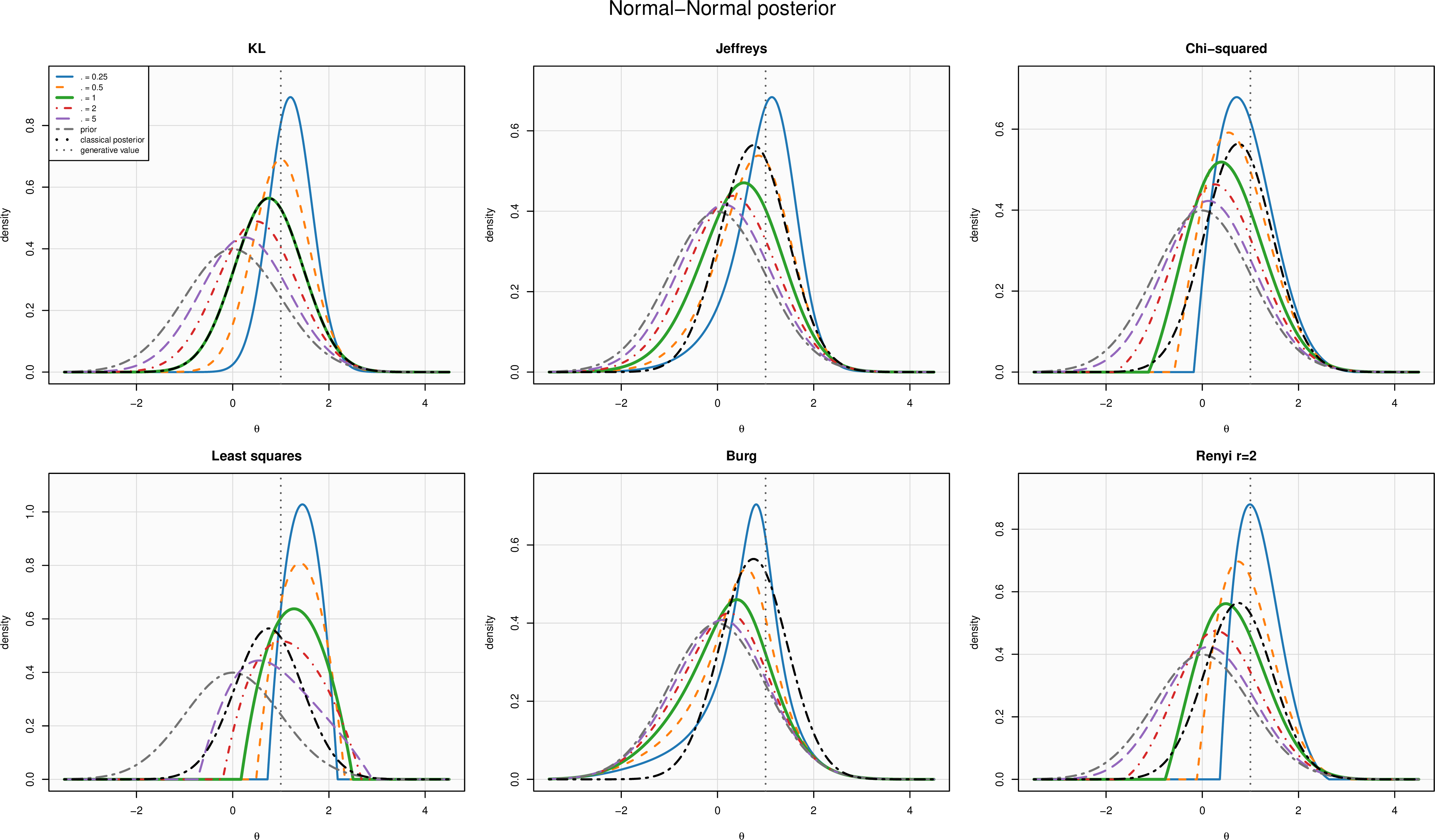
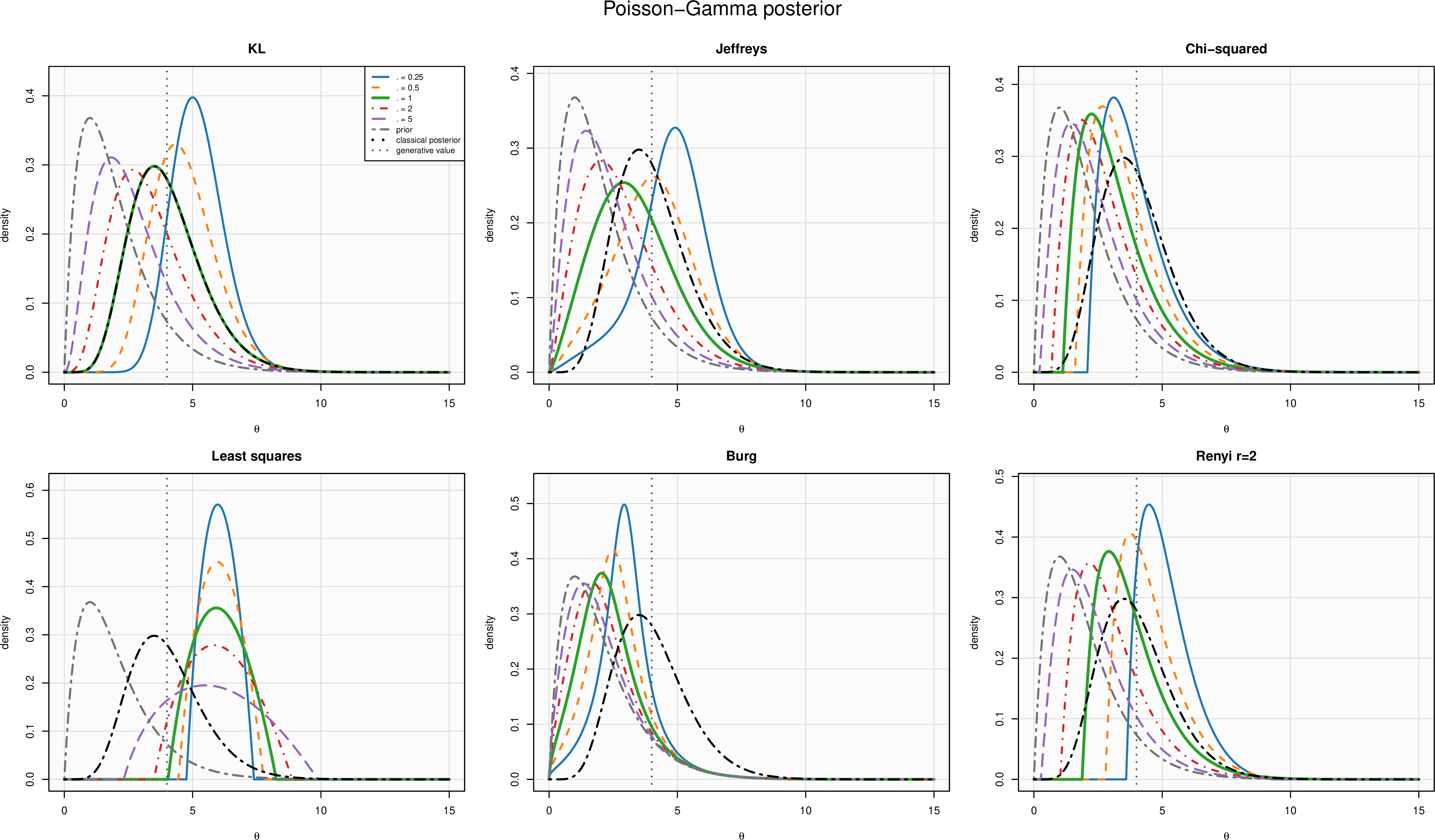
Figures 1 and 2 show that changing the divergence affects more than the effective temperature of the likelihood. In the \(\mathsf{KL}\) panel, changing \(\alpha\) produces the familiar exponential tilting of the prior by the likelihood loss, and the \(\alpha=1\) curve coincides with the classical posterior. The Pearson \(\chi^2\), least-squares, and order-two Rényi panels display the positive-part structure of the formulas in Sections 3, 4, and 5. By contrast, Jeffreys and Burg/Itakura–Saito regularization retain positive densities in these examples but reweight the prior through nonlinear ratio or density coordinates.
8 Conclusion↩︎
Exact GVI solutions exist beyond the \(\mathsf{KL}\)/Gibbs case. These formulas can make non-\(\mathsf{KL}\) GVI analytically tractable and can also serve as inputs to downstream asymptotic questions, such as posterior consistency, Bernstein–von Mises limits, and large-sample limits of posterior functionals, in the spirit of existing generalized-posterior theory [39], [40]. Natural extensions include projection of the closed-form solutions onto tractable variational families, development of stochastic or deterministic solvers for the scalar multiplier, and analysis of their numerical and statistical properties. We leave these directions to future work.
Acknowledgements↩︎
The authors thank Julyan Arbel and Thomas Guilmeau for helpful discussions.
Supplementary Materials
Closed-form solutions to some generalized variational inference problems
9 Foundational facts↩︎
The following facts are used as convex-analytic and scalar-normalization background behind our technical statements.
Lemma 1 (Fenchel–Young equality). Let \(g:\mathbb{R}\to(-\infty,\infty]\) be proper, LSC, and convex. Then \(g(t)+g^*(y)\ge ty\) for all \(t,y\in\mathbb{R}\), and equality holds if and only if \(y\in\partial g(t)\).
Proof. This is the Fenchel–Young inequality; see [21]. ◻
Lemma 2 (Separable convex integral optimality). Let \((\mathcal{Z},\mathfrak{Z},\nu)\) be a measure space, let \(I\subseteq\mathbb{R}\) be an interval, and let \(H:\mathcal{Z}\times I\to(-\infty,\infty]\) be measurable in \(z\) and proper, LSC, strictly convex, and coercive in \(t\in I\). If, for some \(\lambda^\star\in\mathbb{R}\), a measurable function \(t_{\lambda^\star}\) minimizes \(H(z,t)+\lambda^\star t\) pointwise over \(I\) and satisfies \(\int_{\mathcal{Z}}t_{\lambda^\star}\,\mathrm{d}\nu=1\), then \(t_{\lambda^\star}\) minimizes \(\int_{\mathcal{Z}}H(z,t(z))\,\mathrm{d}\nu\) over measurable \(t\) satisfying \(\int_{\mathcal{Z}}t\,\mathrm{d}\nu=1\). The minimizer is unique up to \(\nu\)-a.e. equality whenever equality in the objective is attained by another feasible function.
Proof. For every feasible measurable \(t\), pointwise optimality gives \[H(z,t(z))+\lambda^\star t(z)\ge H(z,t_{\lambda^\star}(z))+\lambda^\star t_{\lambda^\star}(z)\] for \(\nu\)-a.e. \(z\). After integration, the two multiplier terms are both equal to \(\lambda^\star\) by the mass constraint, so \(t_{\lambda^\star}\) has objective value no larger than that of \(t\). If another feasible \(t\) attains the same value, then the pointwise inequality must be an equality \(\nu\)-a.e. on the set where the integrals are finite. Strict convexity of the scalar objective gives \(t=t_{\lambda^\star}\) \(\nu\)-a.e. ◻
Lemma 3 (Lagrange multiplier for the mass constraint). For the affine set of densities \(\{u:\int_{\mathcal{Z}}u\,\mathrm{d}\nu=1\}\), the Lagrange multiplier for the mass constraint is represented by a constant function. Thus the first-order condition for a separable integrand contains a scalar additive term \(\lambda\).
Proof. Adding a scalar multiple of the mass constraint changes the objective by \(\lambda\int_{\mathcal{Z}}u\,\mathrm{d}\nu\). On the feasible set this quantity is the constant \(\lambda\), so it does not change which feasible density minimizes the objective. The scalar \(\lambda\) is chosen so that the pointwise minimizer of the modified integrand has total mass one. Equivalently, for any two feasible densities \(u\) and \(v\), \(\lambda\int_{\mathcal{Z}}(v-u)\,\mathrm{d}\nu=0\), which is why only a constant additive term appears in the scalar first-order condition. ◻
Lemma 4 (Normalizing multiplier). Let \((\mathcal{Z},\mathfrak{Z},\nu)\) be a measure space, let \(h:\mathcal{Z}\to\mathbb{R}\) be measurable, and let \(\Phi:\mathbb{R}\to[0,\infty)\) be continuous, nonincreasing, and strictly decreasing on \(\{x:\Phi(x)>0\}\). Suppose \[G(\lambda)=\int_{\mathcal{Z}}\Phi(h(z)+\lambda)\,\nu(\mathrm{d}z)<\infty \quad\text{for all }\lambda\in\mathbb{R}.\] Then \(G\) is continuous and nonincreasing, and each positive level set \(G^{-1}(\{c\})\), \(c>0\), contains at most one point. If, additionally, \[\lim_{\lambda\to\infty}G(\lambda)=a,\qquad \lim_{\lambda\to-\infty}G(\lambda)=b,\] with \(0\le a<b\le\infty\), then for every \(c\in(a,b)\) there is a unique \(\lambda\) such that \(G(\lambda)=c\).
Proof. Monotonicity of \(G\) follows from monotonicity of \(\Phi\). To prove continuity, fix \(\lambda\in\mathbb{R}\) and choose \(\delta>0\). For \(|\eta|\le\delta\), \[0\le \Phi(h+\lambda+\eta)\le \Phi(h+\lambda-\delta),\] because \(\Phi\) is nonincreasing. The right-hand side is integrable by the hypothesis \(G(\lambda-\delta)<\infty\). Since \(\Phi\) is continuous, dominated convergence gives \(G(\lambda+\eta)\to G(\lambda)\) as \(\eta\to0\).
For uniqueness, suppose \(\lambda_1<\lambda_2\) and \(G(\lambda_1)=G(\lambda_2)=c>0\). Let \(A=\{z:\Phi(h(z)+\lambda_2)>0\}\). Since \(G(\lambda_2)=c>0\), \(\nu(A)>0\). On \(A\), monotonicity gives \(\Phi(h+\lambda_1)\ge\Phi(h+\lambda_2)>0\), so both arguments lie in the positivity set of \(\Phi\). Strict decrease on this set gives \(\Phi(h+\lambda_1)>\Phi(h+\lambda_2)\) on \(A\), while monotonicity gives the same weak inequality on \(\mathcal{Z}\setminus A\). Hence \(G(\lambda_1)>G(\lambda_2)\), a contradiction.
If the endpoint limits are \(a\) and \(b\) with \(0\le a<b\le\infty\), continuity and monotonicity imply that the range of \(G\) contains every \(c\in(a,b)\). The uniqueness just proved completes the argument. ◻
10 Proof of Theorem 1 and Corollary 1↩︎
Fix \(\lambda\in\mathbb{R}\) and \(z\in\mathcal{Z}\). The scalar map \[t\mapsto \alpha f(t)+(\ell(z)+\lambda)t\] is proper, LSC, and strictly convex on \([0,\infty)\). The assumption \(f'_-(\infty)=\infty\) implies that the derivative of this scalar objective tends to \(\infty\) as \(t\to\infty\), hence the objective is coercive and has a unique minimizer. If the minimizer is positive, differentiability gives \[\ell(z)+\lambda+\alpha f'(u_\lambda(z))=0.\] If the minimizer is zero, the one-sided optimality condition is \[\ell(z)+\lambda+\alpha f'_+(0)\ge0,\] equivalently \(-(\ell(z)+\lambda)/\alpha\le f'_+(0)\). This proves 5 . Since the scalar solution is obtained by applying a monotone inverse, with possible clipping at zero, to the measurable function \(\ell+\lambda\), it is measurable.
It remains to show that the scalar minimizer can be normalized. Define \[G(\lambda)=\int_{\mathcal{Z}}u_\lambda\,\mathrm{d}P.\] Since \(\ell\) is bounded below, say \(\ell\ge m\) \(P\)-a.s., the formula 5 gives \[0\le u_\lambda(z)\le \max\left\{0,(f')^{-1}\!\left(-\frac{m+\lambda}{\alpha}\right)\right\}\] with the obvious interpretation when the inverse branch is inactive. Hence \(G(\lambda)<\infty\) for every finite \(\lambda\). The map \(\lambda\mapsto u_\lambda(z)\) is continuous and nonincreasing, and is strictly decreasing whenever it is positive. Lemma 4 implies that \(G\) is continuous and that each positive level set contains at most one point. As \(\lambda\to\infty\), \(u_\lambda(z)\to0\) pointwise and dominated convergence gives \(G(\lambda)\to0\). As \(\lambda\to-\infty\), \(u_\lambda(z)\to\infty\) for \(P\)-a.e. \(z\) with finite \(\ell(z)\), and this set has \(P\)-mass one because \(\ell\in\mathcal{L}^1(P)\). Monotone convergence gives \(G(\lambda)\to\infty\). Lemma 4 therefore gives a unique \(\lambda^\star\) such that \(G(\lambda^\star)=1\).
Let \(u\in\mathcal{U}\). Applying Lemma 1 with \(y=-(\ell+\lambda)/\alpha\) yields, \(P\)-a.s., \[f(u)+f^*\!\left(-\frac{\ell+\lambda}{\alpha}\right) \ge -\frac{\ell+\lambda}{\alpha}u.\] Multiplying by \(\alpha\) and integrating over \(\mathcal{Z}\) gives \[\int_{\mathcal{Z}}\{\ell u+\alpha f(u)\}\,\mathrm{d}P \ge -\lambda\int_{\mathcal{Z}}u\,\mathrm{d}P - \alpha\int_{\mathcal{Z}}f^*\!\left(-\frac{\ell+\lambda}{\alpha}\right)\,\mathrm{d}P.\] Since \(\int_{\mathcal{Z}}u\,\mathrm{d}P=1\), this is the weak dual bound \[\int_{\mathcal{Z}}\{\ell u+\alpha f(u)\}\,\mathrm{d}P \ge -\lambda- \alpha\int_{\mathcal{Z}}f^*\!\left(-\frac{\ell+\lambda}{\alpha}\right)\,\mathrm{d}P.\] Taking the supremum over \(\lambda\) gives weak duality, in the sense that the primal infimum is bounded below by the supremum of the displayed dual lower bounds.
At \(\lambda=\lambda^\star\), the density \(u_{\lambda^\star}\) belongs to \(\mathcal{U}\). By construction, \(u_{\lambda^\star}(z)\) minimizes \(t\mapsto\alpha f(t)+(\ell(z)+\lambda^\star)t\). Equivalently, for \(P\)-a.e. \(z\), the value \(y_z=-(\ell(z)+\lambda^\star)/\alpha\) belongs to \(\partial f(u_{\lambda^\star}(z))\), with the boundary case \(u_{\lambda^\star}(z)=0\) interpreted through the one-sided subgradient condition. Hence Fenchel–Young is an equality \(P\)-a.s., \[f(u_{\lambda^\star})+f^*\!\left(-\frac{\ell+\lambda^\star}{\alpha}\right) =-\frac{\ell+\lambda^\star}{\alpha}u_{\lambda^\star}.\] Therefore the weak dual bound is attained by \(u_{\lambda^\star}\). This proves optimality and the dual identity in Corollary 1. The supremum in 7 is attained at \(\lambda^\star\).
If another feasible \(u\) also attained the minimum, equality in the weak dual bound at \(\lambda^\star\) would be necessary. Equality in Fenchel–Young would then hold for \(P\)-a.e. \(z\). Since the scalar minimizer is unique, \(u(z)=u_{\lambda^\star}(z)\) for \(P\)-a.e. \(z\). This proves uniqueness.
11 Derivations for the \(f\)-divergence examples↩︎
For \(\mathsf{KL}\), \(f'(t)=\log t\) and \(u_\lambda=e^{-(\ell+\lambda)/\alpha}\). Normalization gives \[e^{-\lambda/\alpha}=\left(\int_{\mathcal{Z}}e^{-\ell/\alpha}\,\mathrm{d}P\right)^{-1},\] which is 8 . For Pearson \(\chi^2\), \(f'(t)=2(t-1)\), so the unconstrained solution is \(1-(\ell+\lambda)/(2\alpha)\) and the constraint \(t\ge0\) gives the positive part in 9 .
For squared Hellinger, the Lagrangian integrand is \[(\ell+\lambda)t+\alpha(\sqrt t-1)^2 = (\ell+\lambda+\alpha)t-2\alpha\sqrt t+\alpha.\] Let \(c=\ell+\lambda+\alpha\). If \(c>0\), then \[ct-2\alpha\sqrt t=\left(\sqrt c\sqrt t-\frac{\alpha}{\sqrt c}\right)^2-\frac{\alpha^2}{c},\] with equality at \(t=\alpha^2/c^2\). Choosing \(\lambda=\lambda^\star\) satisfying the normalization condition gives 14 . Strict convexity of \(t\mapsto(\sqrt t-1)^2\) on \((0,\infty)\) and the equality argument above give uniqueness. If \(c<0\) on a set of positive \(P\)-mass, the scalar objective tends to \(-\infty\) as \(t\to\infty\) on that set; if \(c=0\), it tends to \(-\infty\) as \(\sqrt t\to\infty\). Hence the positivity condition is the condition under which the displayed scalar minimizer is meaningful.
12 Proof of the reverse \(f\)-divergence and mixed \(\mathsf{KL}\) formulas↩︎
If \(r=\mathrm{d}Q/\mathrm{d}P>0\), then \(\mathrm{d}P/\mathrm{d}Q=1/r\) and \(\mathrm{d}Q=r\,\mathrm{d}P\), hence \[\mathsf{D}_f(P\Vert Q)=\int_{\mathcal{Z}} f(1/r)r\,\mathrm{d}P =\int_{\mathcal{Z}} f^\diamond(r)\,\mathrm{d}P, \qquad f^\diamond(r)=r f(1/r).\] Convexity of \(f^\diamond\) follows because \((x,t)\mapsto t f(x/t)\) is the perspective of \(f\), restricted to \(x=1\). The proof of 11 is then the proof of Theorem 1 on the open domain \((0,\infty)\), under the corresponding endpoint and normalizing hypotheses for \(f^\diamond\).
For reverse \(\mathsf{KL}\), \(f^\diamond(r)=-\log r+r-1\). The scalar first-order condition \[\ell+\lambda+\alpha(1-1/r)=0\] gives 12 . For the mixed \(\mathsf{KL}\) generator, \[f'_{a,b}(r)=a\log r+b(1-1/r).\] Solving \(f'_{a,b}(r)=-(\ell+\lambda)/\alpha=c\) gives \[a\log r+b-b/r=c.\] Set \(v=b/(ar)\). Then \(\log r=\log(b/a)-\log v\), and the equation becomes \[\log v+v=\log(b/a)+\frac{b-c}{a}.\] Thus \(v e^v=(b/a)\exp((b-c)/a)\) and \[r=\frac{b/a}{\mathrm{W}\left((b/a)\exp((b-c)/a)\right)},\] which is 13 after substituting \(c=-(\ell+\lambda)/\alpha\).
13 Proof of Theorem 2, Corollary 2, and Corollary 3↩︎
For fixed \(\lambda\in\mathbb{R}\) and \(z\in\mathcal{Z}\), the terms depending on \(t\) in the Lagrangian integrand are \[t\mapsto \alpha\psi(t)+(\ell(z)-\alpha\psi'(p(z))+\lambda)t .\] If \(I=[0,\infty)\), the assumptions \(\psi'_-(\infty)=\infty\) and LSC give existence of a minimizer, and strict convexity gives uniqueness. If \(I=(0,\infty)\), the additional assumption \(\psi'_+(0)=-\infty\) implies that the derivative of the scalar objective tends to \(-\infty\) as \(t\downarrow0\), while \(\psi'_-(\infty)=\infty\) implies that the derivative tends to \(+\infty\) as \(t\to\infty\); hence the minimum is attained in the interior of \((0,\infty)\) and is unique.
When the minimizer is interior, the first-order condition is \[\alpha\psi'(q_\lambda(z))+\ell(z)-\alpha\psi'(p(z))+\lambda=0,\] which is 18 . If \(I=[0,\infty)\) and the minimizer occurs at zero, the right-sided derivative at the endpoint is nonnegative: \[\alpha\psi'_+(0)+\ell(z)-\alpha\psi'(p(z))+\lambda\ge0.\] Equivalently, \[\psi'(p(z))-\frac{\ell(z)+\lambda}{\alpha}\le\psi'_+(0),\] which gives the zero branch in the clipped formula 19 . Since the scalar solution is obtained by applying a monotone inverse, with possible clipping at zero, to measurable functions of \(p\) and \(\ell\), the map \(q_\lambda\) is measurable.
Extend \(\psi\) by \(\infty\) outside \(I\) and let \(\psi^*\) denote the Fenchel conjugate of this extended convex function. Put \[b(z)=\ell(z)-\alpha\psi'(p(z)).\] For any feasible density \(q\) in 16 , the Fenchel–Young inequality with \(y=-(b+\lambda)/\alpha\) gives, \(\mu\)-a.e., \[\psi(q)+\psi^*\!\left(-\frac{b+\lambda}{\alpha}\right) \ge -\frac{b+\lambda}{\alpha}q.\] Multiplying by \(\alpha\) and integrating gives \[\int_{\mathcal{Z}}\{\alpha\psi(q)+bq\}\,\mathrm{d}\mu \ge -\lambda\int_{\mathcal{Z}}q\,\mathrm{d}\mu - \alpha\int_{\mathcal{Z}}\psi^*\!\left(-\frac{b+\lambda}{\alpha}\right)\,\mathrm{d}\mu.\] Because \(q\) is feasible, \(\int_{\mathcal{Z}}q\,\mathrm{d}\mu=1\), so \[\int_{\mathcal{Z}}\{\alpha\psi(q)+bq\}\,\mathrm{d}\mu \ge -\lambda - \alpha\int_{\mathcal{Z}}\psi^*\!\left(-\frac{b+\lambda}{\alpha}\right)\,\mathrm{d}\mu.\] This is the weak dual lower bound for 16 .
Now suppose that \(\lambda^\star\) normalizes \(q_{\lambda^\star}\). By the scalar optimality condition defining \(q_{\lambda^\star}\), \[-\frac{b(z)+\lambda^\star}{\alpha} \in \partial\psi(q_{\lambda^\star}(z))\] for \(\mu\)-a.e. \(z\). If \(q_{\lambda^\star}(z)=0\) in the case \(I=[0,\infty)\), this inclusion means \[-\frac{b(z)+\lambda^\star}{\alpha}\le\psi'_+(0),\] which is the right-sided subgradient condition for the extended convex function at the endpoint \(0\). Hence Fenchel–Young is an equality at \(q_{\lambda^\star}\), and the weak dual lower bound is attained by \(q_{\lambda^\star}\). Therefore \(q_{\lambda^\star}\) is a global minimizer of 16 , and taking the supremum over \(\lambda\) gives the dual identity in Corollary 3.
If another feasible density \(q\) also attained the same minimum, equality in the weak dual bound at \(\lambda^\star\) would be necessary. Equality in Fenchel–Young would then hold for \(\mu\)-a.e. \(z\). Since the scalar minimizer in 17 is unique, \(q=q_{\lambda^\star}\) \(\mu\)-a.e. This proves uniqueness. Corollary 2 follows by applying Lemma 4 to \(G(\lambda)=\int_{\mathcal{Z}}q_\lambda\,\mathrm{d}\mu\).
The least-squares and density-power examples follow by substituting \(\psi'(t)=t\) and \(\psi_\beta'(t)=t^\beta/\beta\), respectively. For Burg/Itakura–Saito, \(\psi(t)=-\log t\) gives the scalar objective \[-\alpha\log t+\left(\ell(z)+\lambda+\frac{\alpha}{p(z)}\right)t,\] whose derivative vanishes at \[t=\frac{1}{p(z)^{-1}+(\ell(z)+\lambda)/\alpha} =\frac{\alpha p(z)}{\alpha+p(z)(\ell(z)+\lambda)}.\] Normalization gives 23 ; strict convexity gives uniqueness.
14 Proof of Theorem 4↩︎
Let \(S(u)=\int_{\mathcal{Z}}u^r\,\mathrm{d}P\) and assume \(u^\star\) is a global minimizer with \(0<S(u^\star)<\infty\).
For \(n\ge1\), set \(B_n=\{u^\star\ge 1/n\}\). Let \(h\) be bounded, measurable, supported in \(B_n\), and satisfy \(\int_{\mathcal{Z}}h\,\mathrm{d}P=0\). For all sufficiently small \(|\varepsilon|\), the density \(u^\star+\varepsilon h\) is nonnegative and integrates to one. The map \[\varepsilon\mapsto \int_{\mathcal{Z}}\ell(u^\star+\varepsilon h)\,\mathrm{d}P +\frac{\alpha}{r-1}\log\int_{\mathcal{Z}}(u^\star+\varepsilon h)^r\,\mathrm{d}P\] has a minimum at \(\varepsilon=0\). Differentiation under the integral is justified by boundedness of \(h\), the lower bound \(u^\star\ge1/n\) on the support of \(h\), and the finiteness of \(S(u^\star)\). Hence \[0=\int_{B_n}\left[\ell+ \frac{\alpha r}{r-1}\frac{(u^\star)^{r-1}}{S(u^\star)}\right]h\,\mathrm{d}P.\] The bracketed term is therefore constant on \(B_n\). Since \(B_n\uparrow B=\{u^\star>0\}\) and the constants agree on overlaps, there is \(\lambda^\star\in\mathbb{R}\) such that \[\ell(z)+\frac{\alpha r}{r-1}\frac{u^\star(z)^{r-1}}{S(u^\star)}=\lambda^\star \quad\text{for }P\text{-a.e. }z\in B.\] Thus on \(B\), \[u^\star(z)=k(\lambda^\star-\ell(z))^{1/(r-1)}, \qquad k=\left(\frac{r-1}{\alpha r}S(u^\star)\right)^{1/(r-1)}.\] In particular, \(\ell<\lambda^\star\) on \(B\). Since \(u^\star\) has total mass one, \(P(B)>0\), and therefore \(\lambda^\star>\operatorname*{ess\,inf}_{P}\ell\).
It remains to identify the zero set. Let \(C\subseteq B^c\) be measurable. Choose a measurable \(E\subseteq B\) with \(0<P(E)<\infty\) and \(u^\star\) bounded away from zero on \(E\); such an \(E\) exists because \(\int_{\mathcal{Z}}u^\star\,\mathrm{d}P=1\). For \(P(C)>0\), use the right-sided feasible perturbation \[h=\frac{\mathbf{1}_C}{P(C)}-\frac{\mathbf{1}_E}{P(E)}.\] For sufficiently small \(\varepsilon>0\), \(u^\star+\varepsilon h\) is feasible. The one-sided derivative at zero is nonnegative. On \(C\), the derivative of the \(\mathcal{L}^r\) term is zero because \(r>1\) and \(u^\star=0\) there; on \(E\), the bracketed first-order term equals \(\lambda^\star\). Hence \[0\le \frac{1}{P(C)}\int_C(\ell-\lambda^\star)\,\mathrm{d}P.\] Since this holds for every measurable \(C\subseteq B^c\) with positive \(P\)-mass, \(\ell\ge\lambda^\star\) \(P\)-a.e. on \(B^c\). Consequently \[u^\star(z)=k(\lambda^\star-\ell(z))_+^s, \qquad s=\frac{1}{r-1}.\] Normalization gives \(k=1/A_s(\lambda^\star)\), proving 27 . Moreover, \[S(u^\star)=\frac{A_{s+1}(\lambda^\star)}{A_s(\lambda^\star)^r}.\] Combining this with \(k^{r-1}=(r-1)S(u^\star)/(\alpha r)\) yields \[\frac{1}{A_s(\lambda^\star)^{r-1}} = \frac{r-1}{\alpha r}\frac{A_{s+1}(\lambda^\star)}{A_s(\lambda^\star)^r},\] which is equivalent to 28 .
15 Finite-support calculation for order-two Rényi regularization↩︎
For the order-two Rényi regularization, write \(q_i=Q(\{i\})\) and use the uniform prior \(P(\{i\})=1/K\). Then \(u_i=\mathrm{d}Q/\mathrm{d}P(i)=Kq_i\), and \[\int u^2\,\mathrm{d}P=\frac{1}{K}\sum_{i=1}^K K^2q_i^2=K\sum_{i=1}^K q_i^2.\] Hence the finite-dimensional objective is \[F(q)=\sum_{i=1}^K q_i\ell_i+\alpha\log\left(K\sum_{i=1}^K q_i^2\right), \qquad q\in\Delta_K.\] The simplex is compact, \(\sum_i q_i^2>0\) on \(\Delta_K\), and \(F\) is continuous on \(\Delta_K\), so a global minimizer exists.
Let \(A=\{i:q_i>0\}\) be the active set of a candidate minimizer. Substituting \(s=1\) into 27 gives \[q_i=\frac{(\lambda-\ell_i)_+}{\sum_{j=1}^K(\lambda-\ell_j)_+}.\] Thus \(A=\{i:\ell_i<\lambda\}\). On a fixed nonempty active set \(A\), this becomes \[q_i=\frac{\lambda-\ell_i}{\sum_{j\in A}(\lambda-\ell_j)},\quad i\in A, \qquad q_i=0,\quad i\notin A,\] and the threshold equation 28 becomes \[2\alpha\sum_{i\in A}(\lambda-\ell_i)=\sum_{i\in A}(\lambda-\ell_i)^2.\] Equivalently, if \(m=|A|\), \(L_A=\sum_{i\in A}\ell_i\), and \(S_A=\sum_{i\in A}\ell_i^2\), then \(\lambda\) satisfies the quadratic equation \[m\lambda^2-2(L_A+\alpha m)\lambda+S_A+2\alpha L_A=0.\] Only roots satisfying \(\ell_i<\lambda\) for \(i\in A\) and \(\ell_i\ge\lambda\) for \(i\notin A\) are consistent with the chosen active set. If the losses are ordered from smallest to largest, the possible active sets are exactly the first \(k\) losses for \(k=1,\ldots,K\). Evaluating the original objective \(F\) on the finitely many consistent candidates identifies the global minimizer.