The renormalization of the shell-model neutrinoless double-\(\beta\) decay operator starting from effective field theory (I)
June 24, 2026
Abstract
In this work, we approach for the first time the task to perform a shell-model calculation of the matrix element for the neutrinoless double-\(\beta\) decay, within a fully-consistent framework where the expressions of the nuclear Hamiltonian and of the decay operators have been derived through chiral perturbation theory. More precisely, the effective shell-model Hamiltonian and all transition operators have been constructed by way of the many-body perturbation theory, and then employed to calculate both spectroscopic properties of the nuclei involved in the decays under our consideration — namely \(^{48}\)Ca, \(^{76}\)Ge, and \(^{82}\)Se –, as well as the nuclear matrix elements of the electromagnetic and neutrinoless double-\(\beta\) decays. We also present a study of the convergence properties of the calculated matrix elements in order to provide the elements for an estimate of the theoretical uncertainty.
1 Introduction↩︎
During the first decades of this century, the nuclear structure community has seen the rise and consolidation of an innovative approach to the description of atomic nuclei, namely the application of the principles of effective field theory (EFT) to the dynamics ruling the interaction of nucleons in the nuclear environment.
The seeds of such a revolution were planted in a few papers by Steven Weinberg, where it was suggested that nuclei, as low-energy systems, could be studied in terms of pions and nucleons within the framework of EFT [1]–[3]. In such an approach, the long-range component of the nuclear force should be ruled by the symmetries of low-energy QCD – and in particular the spontaneously broken chiral symmetry – and the short-range dynamics is taken into account by a complete set of contact terms, which are proportional to low-energy constants (LECs) that have to be fitted to data.
Chiral perturbation theory (ChPT) has then provided a powerful tool to construct nuclear Hamiltonians with a direct link to the underlying theory for the strong force among hadrons (QCD), and to expand nuclear forces in a consistent structure of two- and many-body components [4], [5].
Moreover, also electroweak currents can be consistently constructed through ChPT, since this framework accounts for the composite nature of hadrons through the symmetries of QCD. As a matter of fact, during the last decade the ChPT expansion of the Gamow-Teller (GT) decay operator has been applied to study standard \(\beta\)-decay processes in different mass regions [6]–[12], and has contributed substantially to the understanding of the nature of the well-known problem of the quenching of the axial coupling constant \(g_A\).
In recent years, EFT has been also applied to construct electroweak currents corresponding to the neutrinoless double-\(\beta\) (\(0\nu\beta\beta\)) decay, performing a ChPT expansion of the two-body current up to next-to-next-to-leading order (N\(^2\)LO) [13]. A relevant feature of the derivation of the \(0\nu\beta\beta\) decay operator within EFT – within the light Majorana-neutrino exchange scenario – is the emergence at the leading order (LO) of a contact operator, that is required to guarantee the renormalizability of the process [13], [14]. Such a short-range component does not appear in the standard expression of the \(0\nu\beta\beta\) operator, that is characterized only by a long-range component [15], [16], and also introduces a new LEC that has to be renormalized by evaluating the \(nn \rightarrow pp e^- e^-\) amplitude [17].
In this paper, we present the results of shell-model (SM) calculations which aim to calculate the nuclear matrix element of the \(0\nu\beta\beta\) decay \(M^{0\nu}\) for a few nuclei of interest – \(^{48}\)Ca, \(^{76}\)Ca, and \(^{82}\)Se –, in terms of effective SM Hamiltonians and decay operators that have been derived from nuclear potentials and \(0\nu\beta\beta\) currents which have been constructed through ChPT.
Our present work is a natural extension of a previous one [12], where we investigated GT transitions involving the same nuclear systems to assess the role of both two-body electroweak currents and many-body correlations as the causes of the well-known issue of the quenching of the axial coupling constant \(g_A\) [18]. In fact, as in Ref. [12], we employ effective SM Hamiltonians (\(H_{\rm eff}\)’s) derived by way of the many-body perturbation theory [19]–[22], starting from the well-known two-nucleon potential constructed by Entem and Machleidt through a chiral perturbative expansion up to N\(^3\)LO [5], [23], and paired by a three-body component that is consistently built at N\(^2\)LO in ChPT.
Consistently with the construction of \(H_{\rm eff}\)’s, we derive effective SM decay operators from two-body current operators at LO in ChPT, and compare the results with those reported in our previous study [24], where the calculations were performed starting from the high-precision CD-Bonn nucleon-nucleon (2N) potential [24], whose repulsive high-momentum components were renormalized through the \(V_{{\rm low}-k}\) procedure [25]. We also confront the outcome of our study with the results reported in a recent paper of Castillo et al., where the authors performed the calculation of \(0\nu\beta\beta\) nuclear matrix elements by way of the nuclear shell model and proton-neutron quasiparticle random-phase approximation (pnQRPA), using two-body decay currents up to N\(^2\)LO in ChPT, but employing phenomenological \(H_{\rm eff}\)’s [26].
This work is organized as follows. In the upcoming Section 2, we report a few details about the expression of the \(0\nu\beta\beta\) decay operator according to the ChPT expansion [13], and highlight the procedure we have followed to derive the effective SM Hamiltonian as well as the \(0\nu\beta\beta\) operator, starting from the chiral 2N N\(^3\)LO potential constructed by Entem and Machleidt [23] and juxtaposed by a three-body component at N\(^2\)LO in ChPT [5].
The results of the SM calculations are then presented in Sec. 3, where first we report the results of low-energy spectroscopic properties of the nuclei involved in the \(0\nu\beta\beta\) decay of \(^{48}\)Ca, \(^{76}\)Ge, and \(^{82}\)Se, to support the reliability of our approach to the SM calculation of electroweak transitions by way of effective Hamiltonians and operators, and validate the nuclear wave functions of the initial and final states. Then, we report the calculated nuclear matrix elements \(M^{0\nu}\)’s, as well as a study of the perturbative behavior of those theoretical values to estimate the theoretical uncertainties that originate from our approach.
The conclusions of this study are drawn in Sec. 4, together with the perspectives of our current project.
2 Theoretical framework↩︎
2.1 ChPT Hamiltonian and \(0\nu\beta\beta\) decay operators↩︎
As mentioned in the Introduction, during the end of 1990s and the dawn of 2000s the application of EFT to low-energy nuclear systems, especially within the ChPT approach, has provided a valuable tool to tackle the problem of generating hadronic interactions in a low-energy regime [4], [5]. The relevant feature of pursuing this approach to the construction of nuclear forces is the link with their underlying theory – the quantum chromodynamics –, that is obtained through the fundamental requirement that any nuclear effective Hamiltonian has to obey to the relevant symmetries of QCD [1].
This framework is based on identifying a separation of the scales between hadronic systems that are characterized by well-defined energy regimes [27]. For finite nuclei the so-called “hard scale’’ is set at \(\Lambda_\chi \sim m_\rho \sim 1\) GeV and the soft scale is then identified with the pion mass – \(Q \sim m_\pi\) –, known also as the chiral-symmetry breaking scale. This represents the building block of the low-energy ChPT expansion, which is arranged in terms of the soft scale over the hard scale, \((Q/\Lambda_\chi)^\nu\), \(Q\) being an external momentum or a pion mass, while the degrees of freedom of the nuclear Hamiltonian are pions and nucleons and, in some cases, (\(\Delta\)) resonances.
As previously reported, for the present study, we have considered a nuclear Hamiltonian consisting of a two- (2NF) and a three-nucleon (3NF) component of the nuclear force. As regards the 2NF component, we choose the high-precision 2N potential developed by Entem and Machleidt through a perturbative expansion at N\(^3\)LO [28]. Consistently, the 2NF potential is paired by a 3NF one, derived at N\(^2\)LO in ChPT, and consisting of three topologies: the two-pion exchange (2PE), one-pion exchange (1PE), and three-nucleon-contact interactions [5]. These terms are specified by a set of LECs that already appear in the 2NF components, but they also contain a new LEC \(c_D\) – associated to the 1PE contribution –, while another new one, \(c_E\) , enters in the 3NF contact potential. These LECs, \(c_D\) and \(c_E\) , should be fixed to reproduce the observables of the \(A=3\) system, and we have adopted the same values as in Refs. [12], [29]–[33], namely \(c_D=-1\) and \(c_E=-0.34\). This choice traces back to a study performed within the no-core shell model (NCSM), where the authors first constrained the relation of \(c_D\)-\(c_E\), and then investigated a set of observables in light \(p\)-shell nuclei to obtain a second constraint [34].
As pointed out in the Introduction, another key feature of ChPT is to provide a tool to construct also electroweak currents consistently with the derivation of the nuclear Hamiltonian, rooting the structure of these decay operators in the symmetries of the QCD and also accounting for the composite structure of nucleons and pions [35]–[40]. This approach has been extensively applied to study GT transitions in light nuclear systems [6]–[10], in a few medium-mass nuclei through ab initio methods [11], and also by way of the realistic shell model [12]. The application of ChPT to the study of \(\beta\) decay has represented a turning point in the understanding of the mechanism of the renormalization of electroweak operators in nuclear systems, and overcoming the so-called “quenching problem” of the axial coupling constant \(g_A\) [41]–[43].
ChPT has been also employed to construct the expression of the \(0\nu\beta\beta\) decay operator induced by the light Majorana-neutrino exchange, shifting the physics of such a process from the energy scale of the lepton-number violation \(\Lambda_{\rm LNV}=1-100\) TeV down the one of low-energy nuclear systems, namely the chiral-symmetry breaking scale [13].
In recent years, the expansion of two- and three-body currents of the \(0\nu\beta\beta\) operator has been carried out in ChPT [13], [44], [45], and a few studies on the impact of this novel approach to the definition of the \(0\nu\beta\beta\) operator has been already conducted by calculating the nuclear matrix elements \(M^{0\nu}\)’s for nuclei that are currently of experimental interest [26], [46]–[48].
As a matter of fact, one of the most relevant features of the definition of the \(0\nu\beta\beta\) decay operator in ChPT is the emergence of a short-range contact operator which is not present in the standard formulation of the theory of \(0\nu\beta\beta\) decay [15], [16]. In the earliest formulation of the EFT approach to defining the light-neutrino exchange mechanism of the \(0\nu\beta\beta\) decay, this contact term appeared as a contribution at N\(^2\)LO of the ChPT expansion [13]. Then, in a following study it has been shown that this contribution had to be promoted at LO of the expansion, to accomplish the need to introduce a counterterm to absorb the ultraviolet (UV) divergences that appear in the calculation of the amplitude of the \(nn \rightarrow pp e^-e^-\) process for \(1S_0 \rightarrow 1S_0\) transitions [14].
As a counterterm, this contribution is regulated by a LEC, dubbed \(g_{\nu}^{\rm NN}\), and the only way to fix it would be by reproducing the data of lepton-number-violation (LNV) processes, data that are not available at present.
In Ref. [14], the authors suggested to estimate the magnitude of the contact term by considering the coefficients of the charge-independence breaking (CIB) contact interaction. For the Entem-Machleidt N\(^3\)LO potential this leads to a value \(g_{\nu}^{\rm NN}=-0.47\) fm\(^2\). It is worth pointing out that Jokiniemi et al. have followed the same considerations in Ref. [47].
As can be seen in the following, these considerations about the contact term, that is intimately connected with the renormalization mechanism of ChPT approach, are very important in the definition of the nuclear matrix element \(M^{0\nu}\).
It should be recalled that the expression of the half-life of a \(0\nu\beta\beta\) decay, assuming the exchange of a light Majorana neutrino, is:
\[\left[ T^{0\nu}_{1/2}\right]^{-1} = G^{0\nu} g_A^4 \left| M^{0\nu} \right|^2 \left|\frac{ \langle m_{\nu}\rangle}{m_e}\right|^2~, \label{halflife}\tag{1}\]
where \(G^{0\nu}\) is the phase-space factor [49], [50], \(M^{0\nu}\) is the nuclear matrix element directly related to the wave functions of the parent and grand-daughter nuclei, \(g_A\) is the axial coupling constant, \(m_e\) is the electron mass, and \(\langle m _{\nu} \rangle = \sum_i (U_{ei})^2 m_i\) is the effective neutrino mass, as expressed in terms of the neutrino masses \(m_i\) and their mixing matrix elements \(U_{ei}\).
At LO in ChPT, \(M^{0\nu}\) is expressed as the sum of a long- and short-range components [13]:
\[M^{0\nu} = M^{0\nu}_{\rm L} + M^{0\nu}_{\rm S} \label{nmeLS}\tag{2}\]
In turn, the formal expression of the LO long-range component \(M^{0\nu}_{\rm L}\) is expressed in terms of the two-body transition-density matrix elements \(\langle f | a^{\dagger}_{p}a_{n} a^{\dagger}_{p^\prime} a_{n^\prime} | i \rangle\), between the initial (\(i\)) and final (\(f\)) nuclear wave functions, as:
\[\begin{align} M_{\rm L \alpha }^{0\nu} & = & \sum_{j_n j_{n^\prime} j_p j_{p^\prime}} \langle f | a^{\dagger}_{p}a_{n} a^{\dagger}_{p^\prime} a_{n^\prime} | i \rangle \nonumber \\ ~ & ~& \times \left< j_p j_{p^\prime} \mid \Theta_{\rm L \alpha} \mid j_n j_{n^\prime} \right>~, \label{M0nuappl} \end{align}\tag{3}\]
where \(\alpha\) stands for Fermi (\(F\)), Gamow-Teller (GT), or tensor (\(T\)) decay channels, and the operators \(\Theta_{\rm L \alpha}\) are [51]:
\[\begin{align} \Theta_{\rm GT} & = & [ \tau^-_{1} \tau^-_{2} (\vec{\sigma}_1 \cdot \vec{\sigma}_2) H_{\rm GT}(r) ]\tag{4} \, , \\ \Theta_{\rm F} & = & \tau^-_{1} \tau^-_{2} H_{\rm F}(r) \tag{5} \, ,\\ \Theta_{\rm T} & = & [\tau^-_{1} \tau^-_{2} \left( 3\left(\vec{\sigma}_1 \cdot \hat{r} \right) \left(\vec{\sigma}_2 \cdot \hat{r} \right) - \right. \nonumber \\ ~ & ~ & \left. \vec{\sigma}_1 \cdot \vec{\sigma}_2 \right) H_{\rm T}(r) ]~, \tag{6} \end{align}\]
The neutrino potentials are expressed as [13]:
\[H_{\alpha}(r)=\frac{2R}{\pi} \int_{0}^{\infty} \frac{j_{n_{\alpha}}(qr) h_{\alpha}(q^2)qdq}{q}~. \label{neutpotappl}\tag{7}\]
It should be pointed out that at LO the expression of \(M^{0\nu}_{\rm L}\), as well as the one of the neutrino potentials in Eq. (7 ), is the same as the one in the standard formulation [15], [16] when resorting to the closure approximation [51], but setting the closure energy equal to zero [13].
Coming back to Eq. (7 ), the nuclear radius \(R\) is defined as \(R=1.2 A^{1/3}\) fm, \(j_{n_{\alpha}}(qr)\) is the spherical Bessel function, \(n_{\alpha}=0\) for Fermi and Gamow-Teller components, while \(n_{\alpha}=2\) for the tensor component.
In the following, we also report the explicit expressions of neutrino form functions, \(h_{\alpha}(q)\), for light-neutrino exchange at LO [13]:
\[\begin{align} h_{\rm F} ({ q}^{2}) & = & g^2_V \, , \nonumber \\ h_{\rm GT} ({ q}^{2}) & = & \left[ 1 - \frac{2}{3} \frac{ { q}^{2}}{ { q}^{2} + m^2_\pi } + \frac{1}{3} ( \frac{ { q}^{2}}{ { q}^{2} + m^2_\pi } )^2 \right] \nonumber\\ && + \frac{2}{3} \frac{g^2_M}{g^2_A} \frac{{ q}^{2} }{4 m^2_p }, \nonumber \\ h_{\rm T} ({ q}^{2}) & = & \left[ \frac{2}{3} \frac{ { q}^{2}}{ { q}^{2} + m^2_\pi } - \frac{1}{3} ( \frac{ { q}^{2}}{ { q}^{2} + m^2_\pi } )^2 \right] \nonumber\\ && + \frac{1}{3} \frac{g^2_M}{g^2_A} \frac{{ q}^{2} }{4 m^2_p } \, , \end{align}\] where \(g_V = 1\), \(g_A \equiv g_A^{free}=1.2723\), \(g_M=(\mu_p - \mu_n)g_V\), and \((\mu_p - \mu_n) = 4.7\).
Then, the full expression of the long-range term (at LO) of the nuclear matrix element \(M^{0\nu}\) is written as \[M^{0\nu}_{\rm L} = M_{\rm GT}^{0\nu} - \frac{g_V^2}{g_A^2} M_{\rm F}^{0\nu} + M_{\rm T}^{0\nu}~~. \label{nme00nu}\tag{8}\]
As regards the short-range contact term, its expression is the same as in Eq. 3
\[\begin{align} M_{\rm S}^{0\nu} & = & \sum_{j_n j_{n^\prime} j_p j_{p^\prime}} \langle f | a^{\dagger}_{p}a_{n} a^{\dagger}_{p^\prime} a_{n^\prime} | i \rangle \nonumber \\ ~ & ~& \times \left< j_p j_{p^\prime} \mid \Theta_{\rm S} \mid j_n j_{n^\prime} \right>~, \label{M0nuappCT} \end{align}\tag{9}\]
where \(\Theta_{\rm S}\) is:
\[\begin{align} \Theta_{\rm S} & = & \tau^-_{1} \tau^-_{2} H_{\rm S}(r) \label{operatorCT} \, , \end{align}\tag{10}\] and the neutrino potential is:
\[H_{\rm S}(r)=\frac{2R}{\pi} \int_{0}^{\infty} j_{0}(qr) h_{\rm S}(q^2)q^2dq~, \label{neutpotappCT}\tag{11}\]
where we choose to regularize the contact term with a Gaussian regulator as in Refs. [26], [47]:
\[h_{\rm S} (q^2) = -2 (g^{\rm NN}_{\nu}/g_A^2) e^{-q^2/(2\Lambda^2)}~. \label{pots}\tag{12}\]
For the sake of consistency, the value of the cutoff is the same as the one chosen for the Hamiltonian regulator \(\Lambda=500\) MeV, and, as previously mentioned, the LEC \(g^{\rm NN}_{\nu} = -0.47\) fm\(^2\), according to Ref. [14] for the Entem-Machleidt 2N potential.
2.2 Effective SM Hamiltonian and transition operators↩︎
In this section we are going to sketch out briefly our approach to the derivation of the effective SM operators that are necessary to construct the nuclear wave functions – namely, the effective SM Hamiltonian \(H_{\rm eff}\) –, and then calculate the nuclear matrix elements that are needed to extract the half-lives of electromagnetic and \(\beta\) decays, the effective SM decay operators \(\Theta_{\rm eff}\)’s.
A more detailed presentation of our approach to the derivation of effective SM Hamiltonians and transition operators by way of the many-body perturbation theory, and starting from realistic nuclear forces, can be found in Refs. [21], [22], [52].
As mentioned in the Introduction, we construct the two \(H_{\rm eff}\)’s, for \(0f1p\) and \(0f_{5/2}1p0g_{9/2}\) model spaces, respectively, from the high-precision 2NF potential developed by Entem and Machleidt through a chiral perturbative expansion at N\(^3\)LO [28] of the EFT Lagrangian, introducing a regulator function whose cutoff parameter is \(\Lambda = 500\) MeV, and that is characterized by a smooth behavior in the high-momentum regime and can be profitably employed for a perturbative derivation of \(H_{\rm eff}\) , as was shown in Refs. [21], [30]. Aside the N\(^3\)LO 2NF component, we include also a 3NF term, which is derived at N\(^2\)LO in the chiral perturbative expansion [5]. The 3NF LECs that do not appear in the 2NF component of the nuclear Hamiltonian, which should be fixed to reproduce the observables of \(A\geq 3\) systems, have been chosen to be \(c_D=-1\) and \(c_E=-0.34\), as introduced in Ref. [34], where the authors identified a set of observables in light \(p\)-shell nuclei that are strongly sensitive to the \(c_D\) value, and then \(c_E\) was constrained to reproduce the binding energies of the \(A=3\) system. We have employed this parametrization also in our preceding works, where the same nuclear Hamiltonian has been considered [12], [29]–[33].
It is also worth noting that the Coulomb potential is explicitly included in the proton-proton channel of the nuclear Hamiltonian.
The procedure to derive \(H_{\rm eff}\) starts from the SM nuclear Hamiltonian \(H\) for \(A\) interacting nucleons, which, by introducing an auxiliary potential \(U\), is split into a one-body term \(H_0\), whose eigenvectors provide the unperturbed SM basis, and an interaction component \(H_1\):
\[\begin{align} H &= & T + V_{\rm 2N} + V_{\rm 3N}= (T+U)+(V_{\rm 2N}+ V_{\rm 3N}-U) \nonumber\\ ~& = &H_{0}+H_{1}~,\label{smham} \end{align}\tag{13}\]
where the auxiliary potential \(U\) is chosen to be the harmonic-oscillator (HO) one, with a value according to the Blomqvist-Molinari formula \(\hbar \omega = 45 A^{-1/3} - 25 A^{-2/3}\) MeV [53], namely \(\hbar \omega = 11\) and 10 MeV for \(^{40}\)Ca and \(^{56}\)Ni cores, respectively .
Since the eigenvalue problem of \(H\) for a many-body system, and within an infinite Hilbert-space of \(H_0\) eigenvectors, cannot be solved, there is the need to construct an effective Hamiltonian by way of a similarity transformation [54], [55] to project the eigenvalue problem into a truncated model space. In our case, we study the double-\(\beta\) decay of \(^{48}\)Ca considering the model space by four proton and neutron orbitals \(0f_{7/2}, 0f_{5/2}, 1p_{3/2}, 1p_{1/2}\), outside \(^{40}\)Ca doubly-closed core. As regards the decays of \(^{76}\)Ge and \(^{82}\)Se, the model space is spanned by the four HO orbitals \(0f_{5/2}, 1p_{3/2}, 1p_{1/2}, 0g_{9/2}\), now considering \(^{56}\)Ni as reference nucleus.
These are the same model spaces as in Ref. [12], where we have performed a study of single- and double-\(\beta\) decays of the same isotopes.
The \(H_{\rm eff}\)’s for these model spaces are derived by way of the time-dependent perturbation theory, namely performing the Kuo-Lee-Ratcliff folded-diagram expansion in terms of the \(\hat{Q}\)-box vertex function [21], [56], [57]:
\[H^{\rm eff}_1 (\omega) = \hat{Q}(\epsilon_0) - P H_1 Q \frac{1}{\epsilon_0 - Q H Q} \omega H^{\rm eff}_1 (\omega) ~,\label{eqfinal}\tag{14}\] where \(\omega\) is the wave operator decoupling the model space \(P\) and its complement \(Q\), and \(\epsilon_0\) is the eigenvalue of the unperturbed degenerate HO Hamiltonian \(H_0\).
We recall that \(\hat{Q}\) box operator is defined as \[\hat{Q} (\epsilon) = P H_1 P + P H_1 Q \frac{1}{\epsilon - Q H Q} Q H_1 P ~, \label{qbox}\tag{15}\] and \(\epsilon\) is an energy parameter called the “starting energy”.
Computationally, it is impossible to perform an exact calculation of the \(\hat{Q}\) box, then the term \(1/(\epsilon - Q H Q)\) is expanded as a power series
\[\frac{1}{\epsilon - Q H Q} = \sum_{n=0}^{\infty} \frac{1}{\epsilon -Q H_0 Q} \left( \frac{Q H_1 Q}{\epsilon -Q H_0 Q} \right)^{n} ~.\]
In all our applications of the many-body perturbation theory to derive \(H_{\rm eff}\), we expand the \(\hat{Q}\) box up to the third order in perturbation theory (n=1) [22], and the set of two-body configurations belonging to the subspace \(Q\) is truncated to those which correspond to an excitation energy smaller than \(E_{\rm max}= N_{\rm max} \hbar \omega\) [21]. In the present paper, we employ the same \(H_{\rm eff}\)’s as in Ref. [12], where all effective SM operators and Hamiltonians have been calculated through \(N_{\rm max} = 18\).
It should be pointed out that we have performed previous studies [30], [58], where it was verified that such a value of \(N_{\rm max}\) is large enough to obtain convergent values of the single-particle (SP) energies and two-body matrix elements of the residual interaction (TBMEs), that is the basic requirement for stable values of the excitation spectra and transition strengths, with a fixed decay operator.
After the \(\hat{Q}\) box is calculated perturbatively, the non-linear matrix equation (14 ) can be solved by way of iterative techniques [54], [59], or graphical non-iterative methods [60].
Usually, SM calculations are performed by a number of valence nucleons that are larger than two, then we include also contributions from induced three-body forces in the calculation of the \(\hat{Q}\) box, namely involving also three valence nucleons, and then resort to a normal-ordering decomposition of the 3NF induced-force contributions arising at second order in perturbation theory. More details of such a method are reported in Refs. [22], [31], but it is worth pointing out that the chosen reference state is the ground state of the nucleus under study, and we consider a fractional filling of model-space orbitals, a procedure that is performed also for the application of the valence-space in-medium similarity transformation group (VS-IMSRG) approach within the “target” normal ordering [61].
We have adopted the normal-ordering decomposition also calculating the contributions at first order in many-body perturbation theory for the calculation of the \(\hat{Q}\) box of the N\(^2\)LO \(3N\) component of the ChPT Hamiltonian [29].
The SM parameters of the \(H_{\rm eff}\)’s that have been employed to study the \(0\nu\beta\beta\) decay of \(^{48}\)Ca, \(^{76}\)Ge, and \(^{82}\)Se – namely the SP energies and the TBMEs of the residual interaction – are included in the Supplemental Material in Ref. [12].
Now, we turn our attention to the derivation of effective SM decay operators \(\Theta_{\rm eff}\)’s.
The need to build effective operators is due to the issue that the diagonalization of the \(H_{\rm eff}\) does not lead to the true nuclear wave-functions, but to their projections onto the model space \(P\). This means that, consistently with the construction of \(H_{\rm eff}\), any decay operator \(\Theta\) has to be renormalized, so that \(\Theta_{\rm eff}\) accounts for the neglected degrees of freedom belonging to the subspace \(Q=1-P\).
As in our previous studies of double-\(\beta\) decay processes [12], [25], [62]–[64], the construction of the effective SM \(0\nu\beta\beta\) operators has been carried out by way of the approach that has been introduced by Suzuki and Okamoto [20], that is consistent with the derivation of \(H_{\rm eff}\).
As for \(H_{\rm eff}\), the derivation of \(\Theta_{\rm eff}\) is grounded on the perturbative expansion of a vertex function, the so-called \(\hat{\Theta}\) box, which is the counterpart of the \(\hat{Q}\) box that has been previously defined in Eq. (15 ). The details of the procedure can be found in Refs. [20], [22], here we are only going to outline the structure of the derivation of any effective SM decay operators \(\Theta_{\rm eff}\) by way of many-body perturbation theory.
As previously mentioned, the perturbative calculation of \(\Theta_{\rm eff}\) starts from introducing two energy-dependent vertex functions:
\[\hat{\Theta} (\epsilon) = P \Theta P + P \Theta Q \frac{1}{\epsilon - Q H Q} Q H_1 P ~,\] \[\hat{\Theta} (\epsilon_1 ; \epsilon_2) = P H_1 Q \frac{1}{\epsilon_1 - Q H Q} Q \Theta Q \frac{1}{\epsilon_2 - Q H Q} Q H_1 P ~,\]
and of their derivatives calculated in \(\epsilon=\epsilon_0\), \(\epsilon_0\) being the eigenvalue of the degenerate unperturbed Hamiltonian \(H_0\):
\[\hat{\Theta}_m = \frac{1}{m!} \frac{d^m \hat{\Theta} (\epsilon)}{d \epsilon^m} \biggl|_{\epsilon=\epsilon_0} ~,\] \[\hat{\Theta}_{mn} = \frac{1}{m! n!} \frac{d^m}{d \epsilon_1^m} \frac{d^n}{d \epsilon_2^n} \hat{\Theta} (\epsilon_1 ;\epsilon_2) \biggl|_{\epsilon_1= \epsilon_0, \epsilon_2 = \epsilon_0} ~\]
Then, a series of operators \(\chi_n\) is calculated:
\[\begin{align} \chi_0 &=& (\hat{\Theta}_0 + h.c.)+ \hat{\Theta}_{00}~~, \tag{16} \\ \chi_1 &=& (\hat{\Theta}_1\hat{Q} + h.c.) + (\hat{\Theta}_{01}\hat{Q} + h.c.) ~~, \tag{17} \\ \chi_2 &=& (\hat{\Theta}_1\hat{Q}_1 \hat{Q}+ h.c.) + (\hat{\Theta}_{2}\hat{Q}\hat{Q} + h.c.) + \nonumber \\ ~ & ~ & (\hat{\Theta}_{02}\hat{Q}\hat{Q} + h.c.)+ \hat{Q} \hat{\Theta}_{11} \hat{Q}~~, \tag{18} \\ &~~~& \cdots \nonumber \end{align}\]
where \(\hat{Q} \equiv \hat{Q}(\epsilon)\).
Finally, \(\Theta_{\rm eff}\) is expressed in the following form: \[\Theta_{\rm eff} = H_{\rm eff} \hat{Q}^{-1} (\chi_0+ \chi_1 + \chi_2 +\cdots) ~, \label{effopexp}\tag{19}\]
where the \(\hat{\Theta}\) function is expanded up to third order in perturbation theory, consistently with the perturbative calculation of the \(\hat{Q}\) box.
It should be noticed that, since the \(0\nu\beta\beta\)-decay operator owns a two-body structure and we are considering nuclear systems with a number of valence nucleons far larger than two, we have included in the \(\hat{\Theta}\) box expansion also leading-order three-body contributions, namely the second-order three-body diagrams that can be found in Refs. [22], [25]. In Ref. [25] we have also discussed the impact of these three-body contributions to the definition of \(\Theta_{\rm eff}\) for the \(0\nu\beta\beta\) decay.
In Refs. [25], [58], [63] there are reported studies of the convergence of the \(\chi_n\) series and of the perturbative properties of the \(\hat{\Theta}\) box, in order to support the robustness of the expansion of \(\Theta_{\rm eff}\).
It is worth pointing out that one of the themes of discussion of the results in Sec. 3 will be the evaluation of theoretical uncertainties associated to our calculated \(M^{0\nu}\)’s of the \(0\nu\beta\beta\) decays of \(^{48}\)Ca, \(^{76}\)Ge, and \(^{82}\)Se, uncertainties that originate from the perturbative expansion of \(H_{\rm eff}\) and \(\Theta_{\rm eff}\).
3 Results↩︎
In this section we present the results of our SM calculations, that are obtained by employing \(H_{\rm eff}\)’s and \(\Theta_{\rm eff}\)’s from ChPT.
First, it is worth considering the quality of the agreement between calculated and experimental spectroscopic properties of the nuclei which are the focus of our study, aiming to assess the quality of the nuclear wave functions we employ to calculate \(M^{0\nu}\)’s. The results of such a study have already been reported in Ref. [12], and in Sec. 3.1 we will report a study of the perturbative properties of \(H_{\rm eff}\)’s and decay \(\Theta_{\rm eff}\)’s.
Then, in Sec. 3.2 we report the results of the calculation of \(M^{0\nu}\)’s for \(^{48}\)Ca, \(^{76}\)Ge, and \(^{82}\)Se decays, considering the \(0\nu\beta\beta\) decay operator at the LO in ChPT expansion. We will present an analysis of the perturbative properties of the \(0\nu\beta\beta\) \(\Theta_{\rm eff}\) to ascertain an uncertainty estimate of the calculated \(M^{0\nu}\)’s, and compare the results with those we obtained in a similar study, in which we have derived \(H_{\rm eff}\)’s and \(\Theta_{\rm eff}\)’s from the meson-theoretic CD-Bonn 2N potential [25].
3.1 Theoretical results vs. experimental quantities↩︎
As already pointed out in the previous sections, our SM calculations are carried out employing theoretical SP energies, TBMEs, and effective transition operators as reported in Sec. 2.2, whose details can be found in Ref. [22].
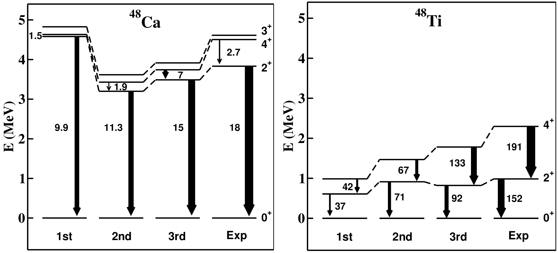
We start considering the nuclei involved in the double-\(\beta\) decay of \(^{48}\)Ca, namely the latter and \(^{48}\)Ti. In Fig. 1, we show the experimental [65] and calculated low-energy spectra of both nuclei, obtained within the full \(fp\) shell, namely the proton and neutron \(0f_{7/2}\), \(0f_{5/2}\), \(1p_{3/2}\), and \(1p_{1/2}\) orbitals. The arrow widths are proportional to the \(B(E2)\) strengths, and next to them we report also the theoretical and experimental values in \(e^2\)fm\(^4\) [65].
Since we want to evaluate the perturbative behavior of the calculated SM effective Hamiltonian, we compare the low-lying excitation spectra obtained with \(H_{\rm eff}\)’s derived at first-, second-, and third-order in many-body perturbation theory. A similar study, performed for one- and two-valence nuclei, was reported in Ref. [30], and here we want to extend it to many-valence nucleon systems.
It should be noticed that in the present study we have employed the same effective \(E2\) transition operator, the one derived at third order in perturbation theory, to calculate \(B(E2)\)’s with \(H_{\rm eff}\)’s that are calculated at different order. In such a way, the focus is spotted on the quality of the shell-model wave functions at each order in perturbation theory, so to recover these information when the attention will be turned to the calculation of \(0\nu\beta\beta\) matrix elements.
As can be seen, the observed shell closure of the neutron \(0f_{7/2}\) orbital in \(^{48}\)Ca is reproduced at all orders, a feature that traces back to the contribution of the three-body component of the nuclear Hamiltonian [30]. The perturbative behavior of the results obtained with second- and third-order \(H_{\rm eff}\)’s is satisfactory, as well as the agreement with experiment. First-order results exhibit some overestimate of the shell closure, that is testified also by the smaller \(B(E2; 2^+_1 \rightarrow 0^+_1)\) with respect to second- and third-order ones.
As regards \(^{48}\)Ti, the strength of the proton-neutron interaction induces a larger collectivity in its low-energy excitation spectrum, also evidenced by larger \(B(E2)\)’s. Second- and third-order \(H_{\rm eff}\)’s reproduce quite well these experimental features, while first-order \(H_{\rm eff}\) is characterized by smaller \(B(E2)\)’s, despite the compressed energy spectrum which usually leads to a larger collectivity.
The calculation of low-energy spectra and wave functions of \(^{76}\)Ge, \(^{76}\)Se, \(^{82}\)Se, and \(^{82}\)Kr has been carried out by employing the four proton and neutron orbitals \(0f_{5/2}\), \(1p_{3/2}\), \(1p_{1/2}\) and \(0g_{9/2}\), outside \(^{56}\)Ni closed core, as model space.
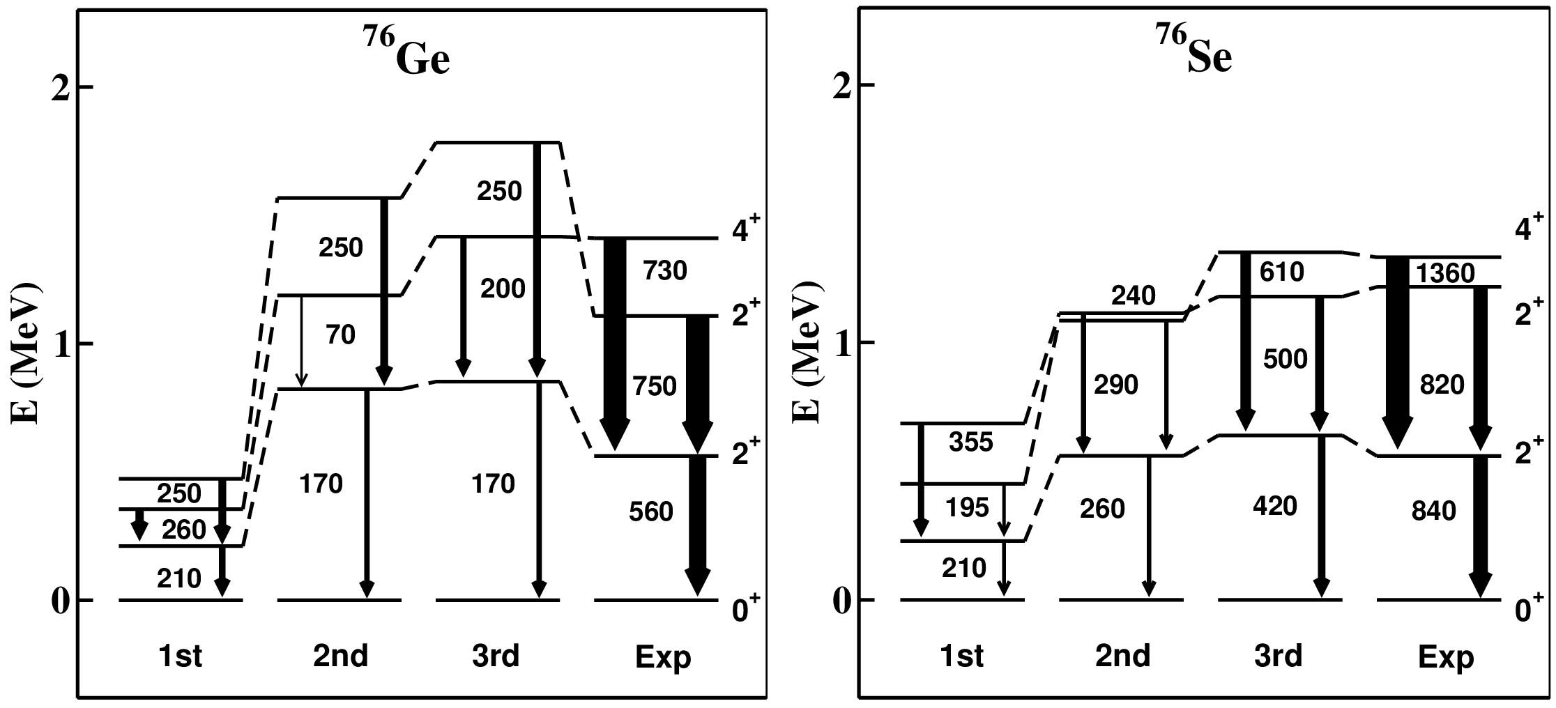
Fig. 2 reports the experimental [65] and calculated low-energy spectra of \(^{76}\)Ge an \(^{76}\)Se, as well as the electric quadrupole transition strengths, following the same scheme of analysis as for \(^{48}\)Ca and \(^{48}\)Ti. It is worth pointing out that the reproduction of the observables characterizing low-energy states in these nuclides is far more challenging for a microscopic nuclear structure model, owing to the experimental evidence of the \(^{76}\)Ge rigid triaxial deformation [66].
First, we observe that there is quite a satisfactory perturbative behavior between second- and third-order \(H_{\rm eff}\)’s , as regards the spectroscopic properties of low-energy states. As regards the agreement with experiment, we have already noticed in Ref. [12] that the agreement between the experimental and calculated spectra and \(B(E2)\)’s for \(^{76}\)Se is very satisfactory, but this is not the same for \(^{76}\)Ge. We have also shown that this traces back to the monopole component of the \(H_{\rm eff}\), especially when comparing with the results obtained in our earlier study where \(H_{\rm eff}\) was derived from a \(V_{{\rm low}-k}\) potential obtained from the CD-Bonn potential [63].
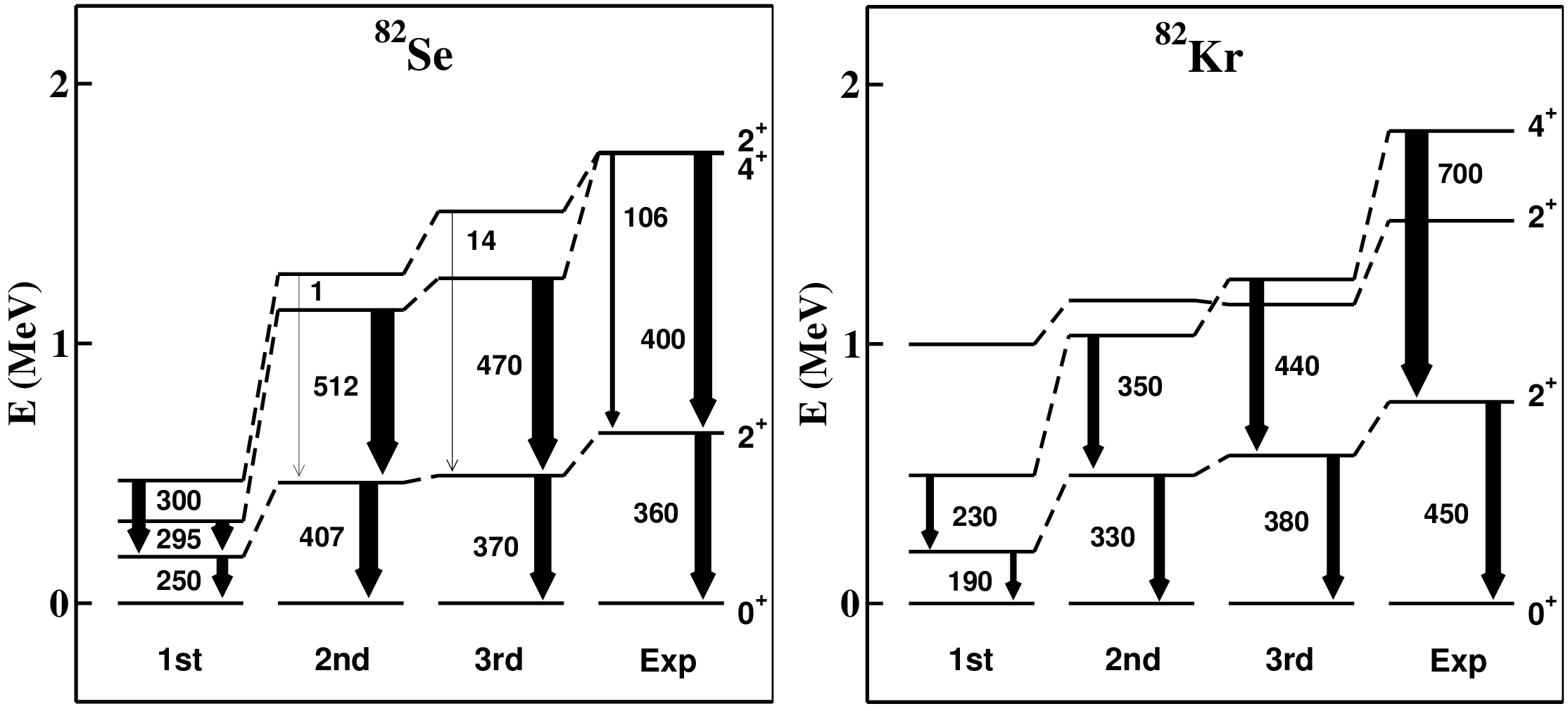
In Fig. 3 we report the results for \(^{82}\)Se and \(^{82}\)Kr low-energy spectra, and compare them with the experimental ones. As can be seen, we have obtained both a good perturbative behavior of the \(H_{\rm eff}\)’s, and a quantitative agreement with observables.
Now, we shift our attention to the results of the matrix elements \(M^{2\nu}\)’s for the two-neutrino double-\(\beta\) decay of \(^{48}\)Ca, \(^{76}\)Ge, and \(^{82}\)Se. The SM effective operator has been constructed by way of ChPT, namely the one- and two-body matrix elements of the axial currents \({\mathbf{J}_A}\) are derived through a chiral expansion up to N\(^3\)LO, and the LECs appearing in their expression are consistent with those of the nuclear potential. The details about the derivation of the SM effective decay operator are reported in Ref. [12], here we have employed the same one – calculated at third order in many-body perturbation theory –, but diagonalizing the SM Hamiltonian with first-, second-, and third-order \(H_{\rm eff}\)’s.
As for the calculation of the \(B(E2)\)’s, our intent is to focus to the perturbative behavior of the SM wave functions, as well as their reliability to reproduce data, within the perspective of the prediction of \(0\nu\beta\beta\) nuclear matrix elements.
| Decay | 1st order | 2nd order | 3rd order | Expt |
| \(^{48}\)Ca\(\rightarrow\)\(^{48}\)Ti | 0.055 | 0.014 | 0.019 | \(0.042 \pm 0.004\) |
| \(^{76}\)Ge\(\rightarrow\)\(^{76}\)Se | 0.022 | 0.056 | 0.118 | \(0.129 \pm 0.004\) |
| \(^{82}\)Se\(\rightarrow\)\(^{82}\)Kr | 0.042 | 0.099 | 0.095 | \(0.103 \pm 0.001\) |
Table ¿tbl:ME952nbb? reports the calculated \(M^{2\nu}\)’s, obtained with the different \(H_{\rm eff}\)’s, for the \(2\nu\beta\beta\) decays \(^{48}\)Ca\(\rightarrow\) \(^{48}\)Ti, \(^{76}\)Ge\(\rightarrow\) \(^{76}\)Se, \(^{82}\)Se\(\rightarrow\) \(^{82}\)Kr (ground state to ground state).
As can be observed, the perturbative behavior is very good for the theoretical \(M^{2\nu}\)’s of \(^{48}\)Ca and \(^{82}\)Se, and less satisfactory for \(^{76}\)Ge, in line with the results for the electric-quadrupole \(B(E2)\)’s. The agreement with experiment is very good considering the third-order \(H_{\rm eff}\), as already pointed out in Ref. [12].
The outcome of the study of the perturbative behavior of the calculated \(H_{\rm eff}\)’s and, most importantly of the calculated SM wave functions, makes us confident that the \(H_{\rm eff}\)’s calculated at third-order in many-body perturbation theory are the best starting point to study the \(0\nu\beta\beta\) decay of \(^{48}\)Ca, \(^{76}\)Ge, and \(^{82}\)Se. Then, in the following section the calculation of \(M^{0\nu}\)’s will be performed by way of third-order \(H_{\rm eff}\)’s to concentrate the attention to the perturbative properties of the SM effective \(0\nu\beta\beta\)-decay operator, and the related uncertainty estimate of the nuclear matrix elements \(M^{0\nu}\)’s.
3.2 Neutrinoless double-\(\beta\) decay of \(^{48}\)Ca, \(^{76}\)Ge, and \(^{82}\)Se↩︎
As introduced in Sec. 2.1, in the present work the calculation of \(M^{0\nu}\) accounts for the light-neutrino exchange mechanism, the total nuclear matrix element being expressed as in Eq. (2 ) and calculated accordingly to Eqs. (4 ,5 ,6 ,10 ,3 ,9 ,7 ,11 ). It should be also recalled that for the short-range contact term we have employed a value of the low-energy constant \(g^{\rm NN}_{\nu}=-0.47\) fm\(^2\), as discussed in Sec. 2.1.
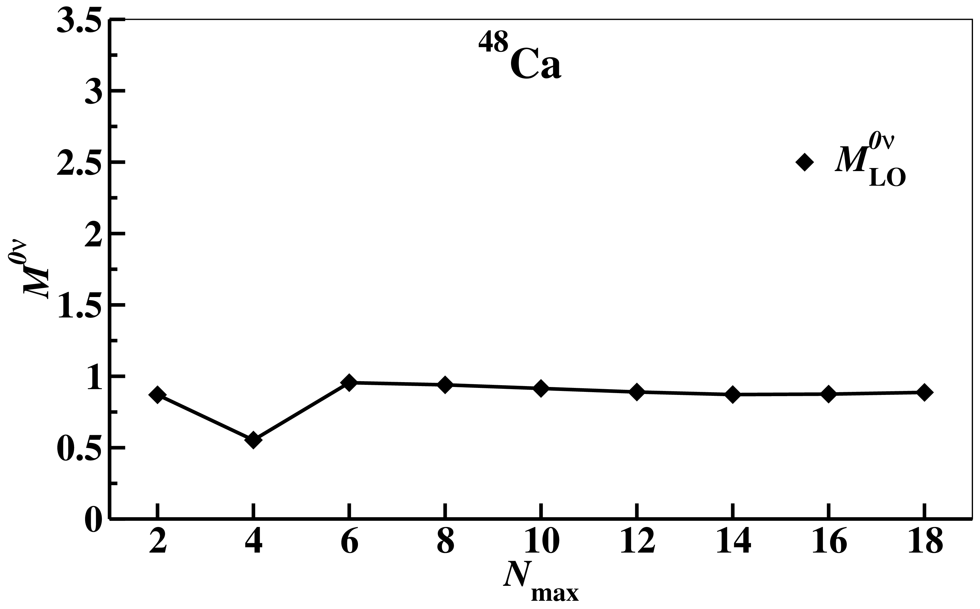
As in our previous studies of the \(0\nu\beta\beta\) decay [25], [64], we have carried out the perturbative expansion of the \(0\nu\beta\beta\) effective operator \(\Theta_{\rm eff}\) including in the \(\hat{\Theta}\) box diagrams up to the third order (see Section 2.2), and a number of intermediate states which corresponds to oscillator quanta up to \(N_{\rm max}=18\). In fact, this value corresponds to a number of intermediate states that is large enough to guarantee a substantial convergence of the calculated \(M^{0\nu}\)’s.
In Fig. 4 the calculated values of \(M^{0\nu}\) for the \({\rm ^{48}Ca} \rightarrow {\rm ^{48}Ti}\) decay are reported as a function of \(N_{\rm max}\), and, as can be observed, results are substantially convergent from \(N_{\rm max}=14\) on.
This convergent behavior appears also for the \(M^{0\nu}\)’s calculated for the \(^{76}\)Ge and \(^{82}\)Se decays, as reported in Table ¿tbl:ME950nbb?.
| Decay | \(N_{\rm max}=14\) | \(N_{\rm max}=16\) | \(N_{\rm max}=18\) |
| \(^{76}\)Ge\(\rightarrow\)\(^{76}\)Se | 1.698 | 1.658 | 1.661 |
| \(^{82}\)Se\(\rightarrow\)\(^{82}\)Kr | 1.284 | 1.250 | 1.253 |
Now, we shift the focus on the results of the order-by-order convergence, that are the starting point for discussing the uncertainties related to our calculated \(M^{0\nu}\)’s.
First, we consider the \(0\nu\beta\beta\) decay between the ground states of \(^{48}\)Ca and \(^{48}\)Ti. In Fig. 5 we have reported the calculated values of \(M^{0\nu}\), \(M^{0\nu}_{\rm GT}\), \(M^{0\nu}_{\rm F}\), \(M^{0\nu}_{\rm T}\), and \(M^{0\nu}_{\rm S}\) from first- up to third-order in perturbation theory. We have decided to report also the value of their Padé approximant \([2|1]\), as an indicator of the quality of the perturbative behavior of the calculated \(M^{0\nu}\) [68].
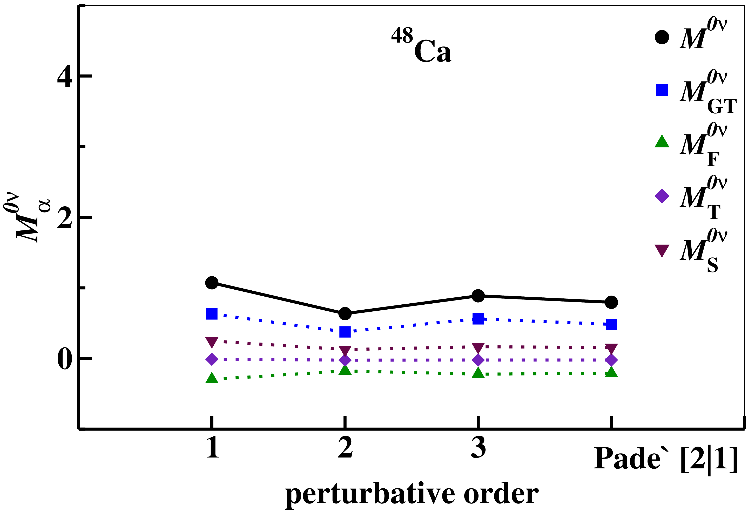
As can be seen in Fig. 5, the perturbative behavior is driven by the Gamow-Teller component, since LO contact term is rather flat between second- and third-order, and both Fermi and tensor matrix elements \(M^{0\nu}_{\rm F}\), \(M^{0\nu}_{\rm T}\) are weakly affected by the renormalization procedure.
A more refined analysis of our results and of the perturbative behavior may be obtained performing a decomposition of \(M^{0\nu}\)’s in terms of the contributions from the decaying pair of neutrons coupled to a given angular momentum and parity \(J^{\pi}\). This decomposition for \(0\nu\beta\beta\) decay of \(^{48}\)Ca is reported in Fig. 6, comparing the contributions obtained by employing the SM effective \(0\nu\beta\beta\)-decay operator \(\Theta_{\rm eff}\) as calculated at first-, second-, and third-order in many-body perturbation theory.
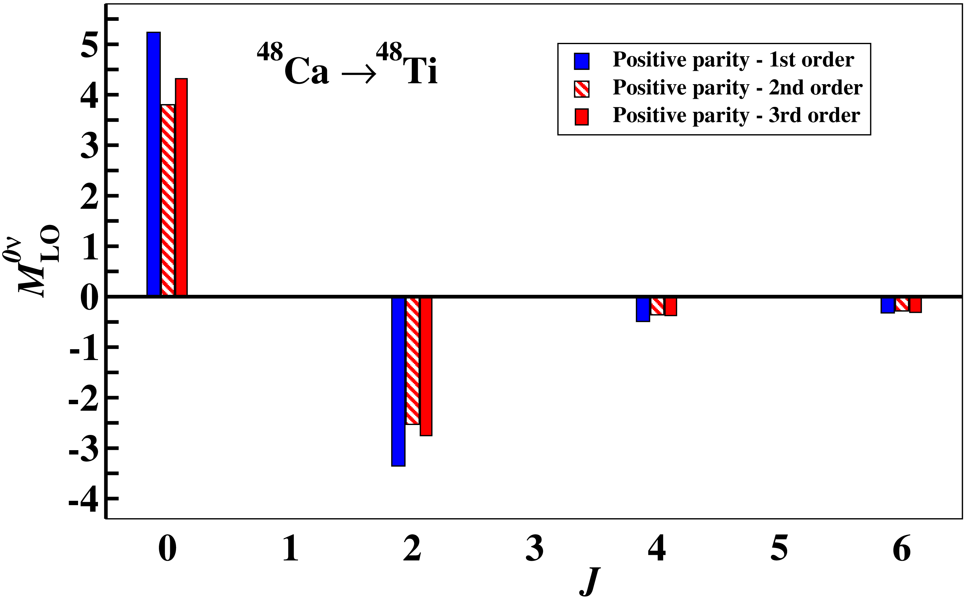
There are two remarks that we point out from the inspection of Fig. 6: first, the main contributions, at all orders, are provided by \(J^{\pi}=0^+,2^+\) components and they are always of opposite sign, and this fact is mainly responsible for the particularly small \(M^{0\nu}\) for the decay of \(^{48}\)Ca, a feature that is common to almost all calculations for this doubly-closed nuclear system [25], [69]–[72].
Second, we note that the perturbative behavior of each component is much better than the total \(M^{0\nu}\), as observed in Fig. 5, and that it is just the cancellation between the two main components which contributes largely to the increase of the uncertainty of the calculated \(M^{0\nu}\), with respect to the one that characterizes each term of the decomposition.
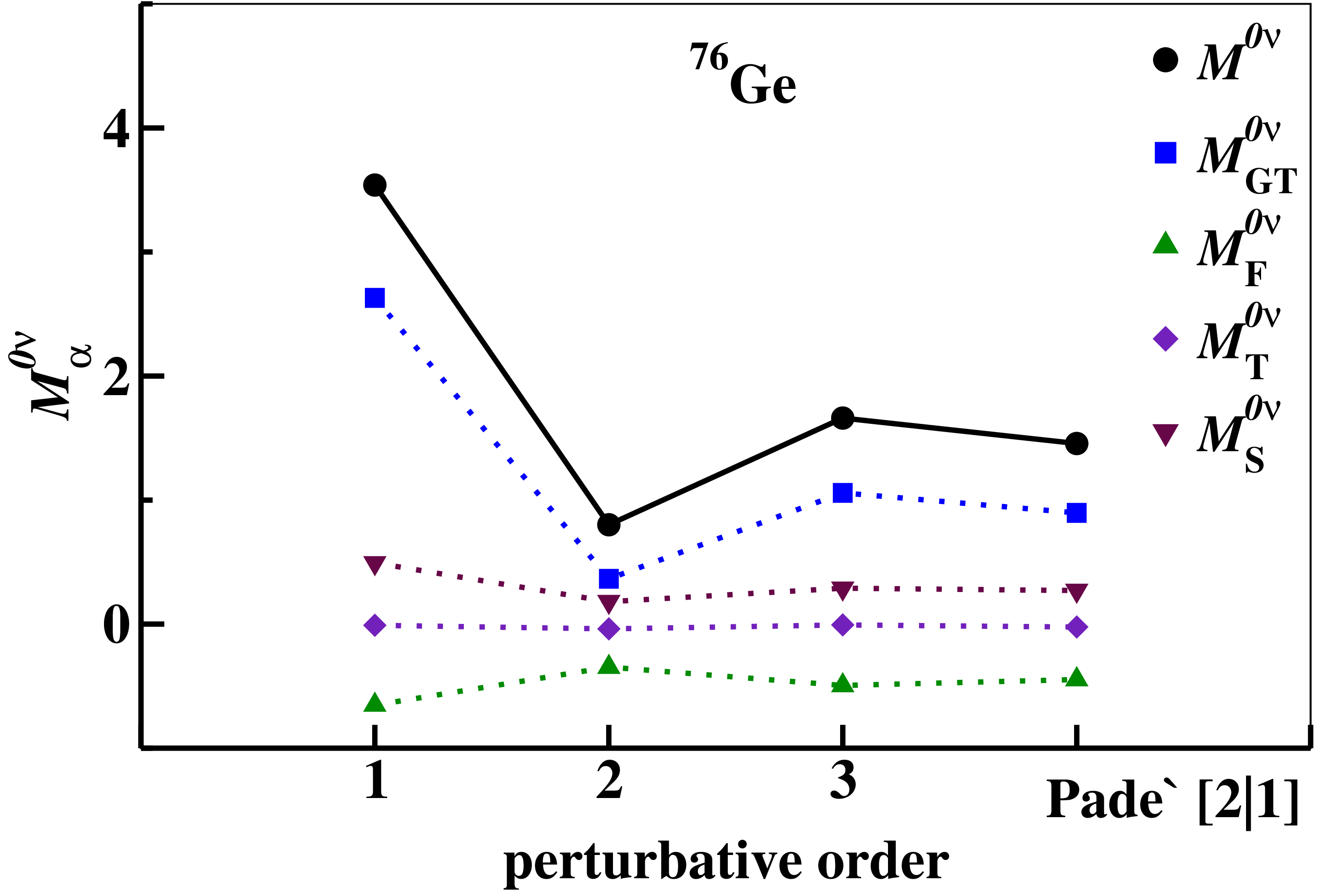
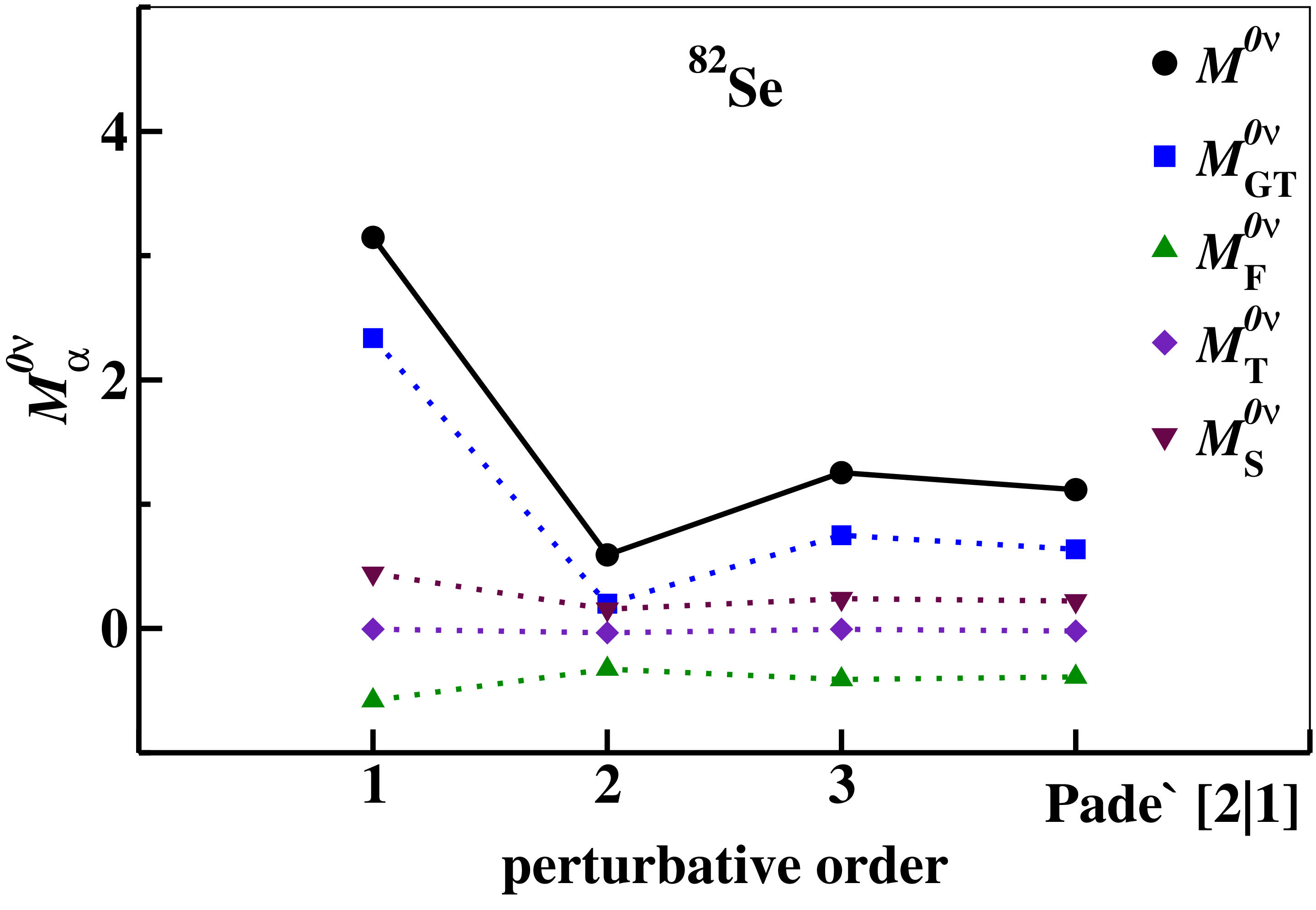
Very similar observations can be drawn also for the \(0\nu\beta\beta\) decay of the ground states of \(^{76}\)Ge, \(^{82}\)Se into the one of \(^{76}\)Se, \(^{82}\)Kr, from the inspection of Figs. 7,8 where they are reported the calculated values of \(M^{0\nu}\), \(M^{0\nu}_{\rm GT}\), \(M^{0\nu}_{\rm F}\), \(M^{0\nu}_{\rm T}\), and \(M^{0\nu}_{\rm S}\) from first- up to third-order in perturbation theory, as well as the value of their Padé approximant \([2|1]\).
For these decays too, the decomposition of \(M^{0\nu}\)’s in terms of the contributions of the decaying pair of neutrons coupled to a given angular momentum and parity \(J^{\pi}\) provides a useful insight on the main sources of the uncertainties related to the perturbative expansion of \(0\nu\beta\beta\) \(\Theta_{\rm eff}\)’s.
From the inspection of Figs. 9,10, we observe that the most relevant contributions come by the \(J^{\pi}=0^+,2^+\) components and they are always of opposite sign, as for the decay of \(^{48}\)Ca, but their respective intensities differ more substantially, and lead to larger \(M^{0\nu}\)’s with respect to the \(^{48}\)Ca decay.
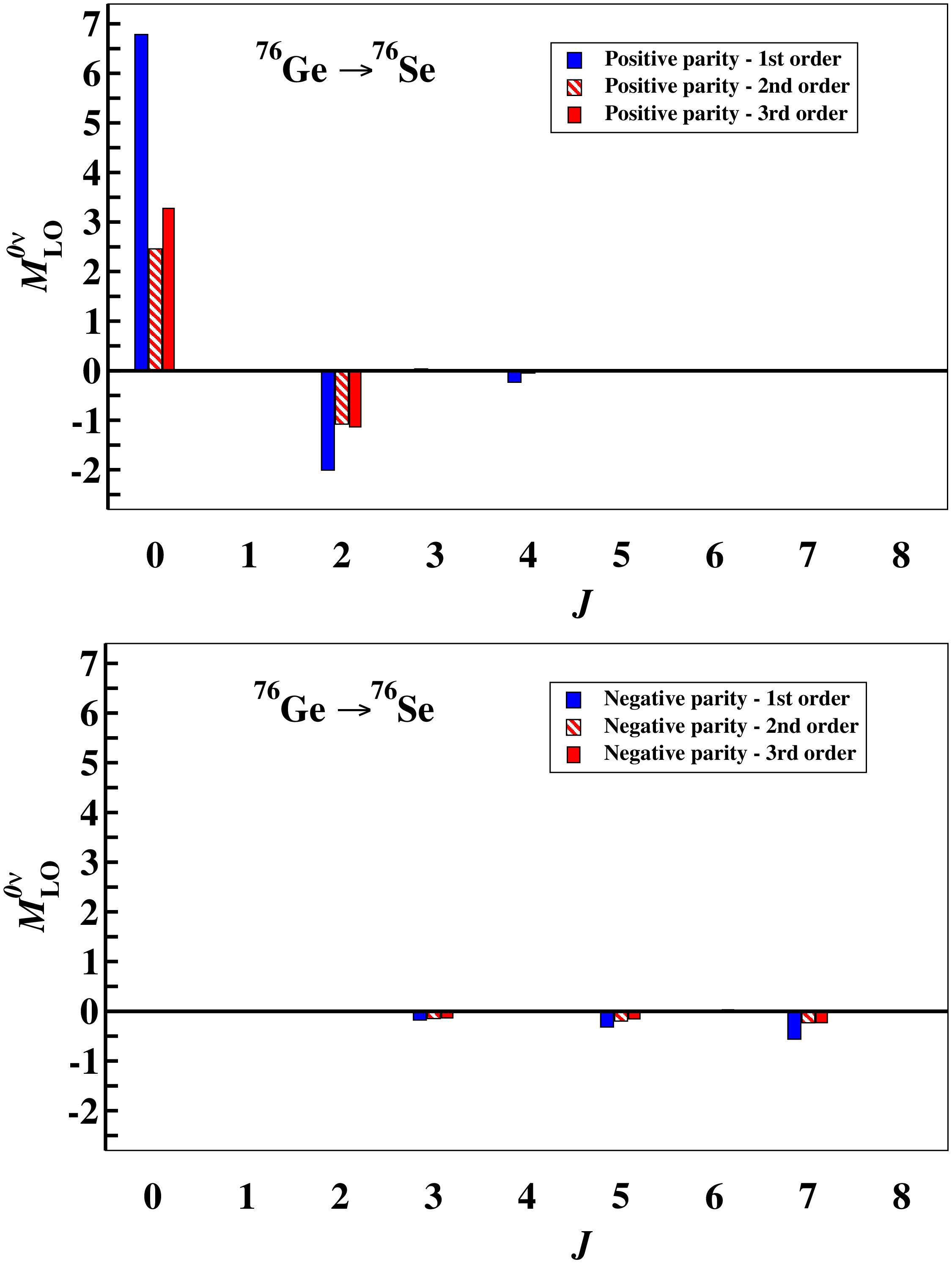
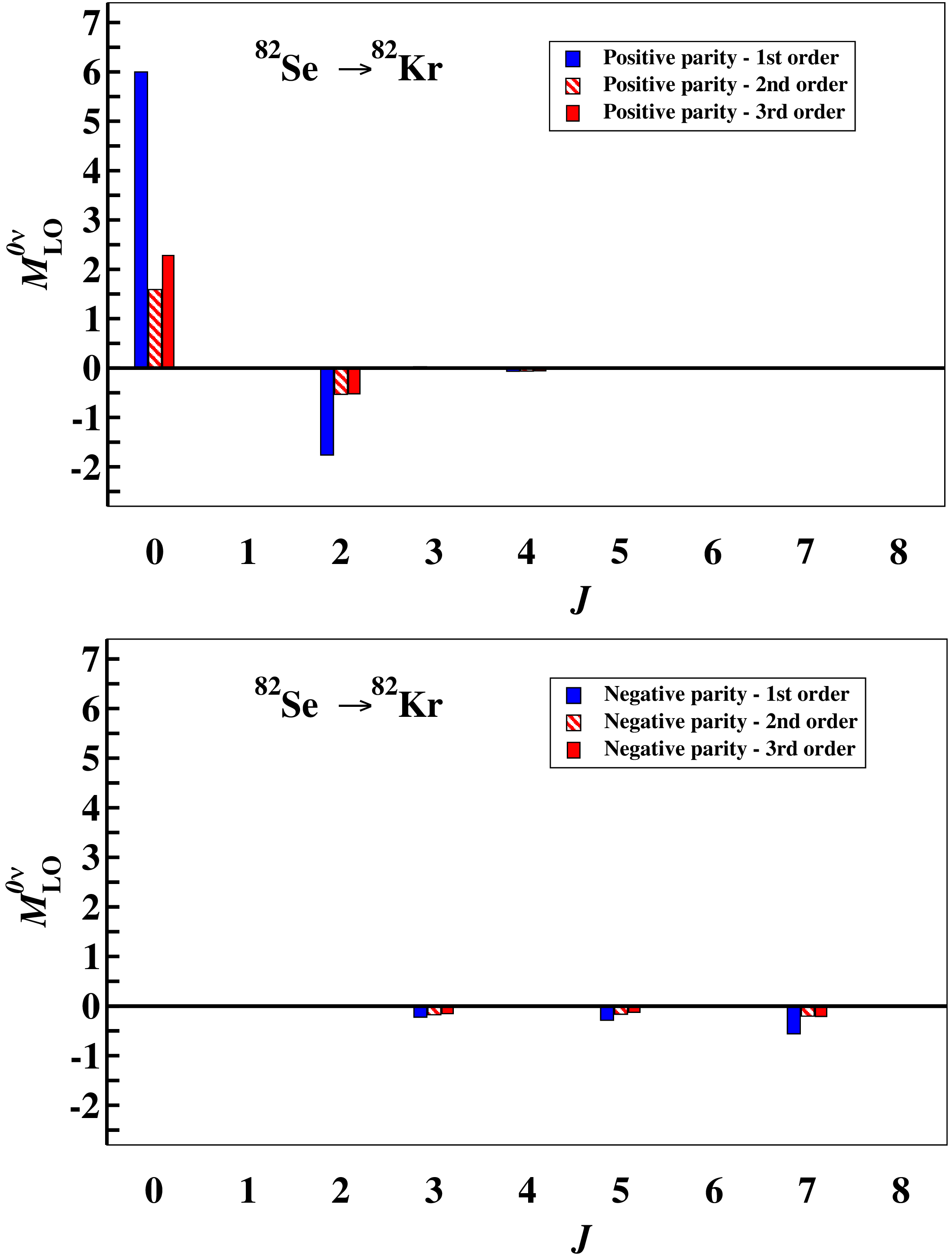
The perturbative behavior is dominated by the \(J^{\pi}=0^+\) component, that is characterized by a larger difference between second- and third-order calculations.
This exposition of our results leads to an analysis of our evaluation of \(M^{0\nu}\)’s for \(^{48}\)Ca, \(^{76}\)Ge, and \(^{82}\)Se \(0\nu\beta\beta\) decays, as well as an estimate of the corresponding theoretical uncertainties.
It should be stressed that a calculation that is grounded on many-body perturbation theory is not a size-extensive approach as for ab initio methods, then a proper theoretical error cannot be evaluated. Then, we rely on the theory of Padé approximant as an instrument to obtain the best approximation of the sum of a perturbative expansion from a truncated power series [68]. Moreover, here we refer only to the many-body perturbation theory as a source of uncertainties, while a complete treatment should involve also a study of the perturbativity of the ChPT expansion of the nuclear Hamiltonian and electroweak currents, the latter defining the decay operators.
| Decay | \(M^{0\nu}_{\rm 3rd}\) | \(M^{0\nu}_{\textrm{Pad\'e}}\) | \(\Delta\) |
| \(^{48}\)Ca \(\rightarrow\) \(^{48}\)Ti | 0.9 (0.89) | 0.8 (0.80) | 0.1 (0.09) |
| \(^{76}\)Ge \(\rightarrow\) \(^{76}\)Se | 1.7 (1.66) | 1.5 (1.46) | 0.2 (0.20) |
| \(^{82}\)Se \(\rightarrow\) \(^{82}\)Kr | 1.3 (1.25) | 1.1 (1.12) | 0.1 (0.13) |
On the above grounds, we have reported in Table ¿tbl:NME? the values of \(M^{0\nu}\)’s as obtained at third order in many-body perturbation theory, and the Padé approximant \([2|1]\) which accounts for the perturbative behavior up to third-order. In the last column, we have reported the absolute value of the difference between these two values \(\Delta=|M^{0\nu}_{\rm 3rd} - M^{0\nu}_{\textrm {Pad\'e}}|\), that we propose as the estimate of the uncertainties associated to our calculated \(M^{0\nu}\)’s.
Finally, it is worth to compare our results with those reported in recent papers, where the \(0\nu\beta\beta\) decay for intermediate- and heavy-mass systems has been investigate within EFT electroweak operators.
| Decay | \(M^{2\nu}_{\rm 3rd}\) | \(M^{2\nu}_{\textrm {Pad\'e}}\) | \(\Delta\) | Expt |
| \(^{48}\)Ca\(\rightarrow\)\(^{48}\)Ti | 0.019 | 0.019 | 0.0 | \(0.042 \pm 0.004\) |
| \(^{76}\)Ge\(\rightarrow\)\(^{76}\)Se | 0.118 | 0.114 | 0.004 | \(0.129 \pm 0.004\) |
| \(^{82}\)Se\(\rightarrow\)\(^{82}\)Kr | 0.095 | 0.093 | 0.002 | \(0.103 \pm 0.001\) |
In Ref. [48], the authors carried out a comprehensive ab initio uncertainty quantification of the \(0\nu\beta\beta\) decay of \(^{76}\)Ge, employing nuclear Hamiltonians and electroweak operators derived within ChPT. \(^{76}\)Ge \(M^{0\nu}\) was calculated with recently developed many-body emulators, and their numerical result is \(M^{0\nu} = 2.60^{+1.28}_{-1.36}\).
The latter is greater than the value reported in Table ¿tbl:NME? – \(M^{0\nu} =1.46\) –, but both \(M^{0\nu}\)’s are consistent within the theoretical error in Ref. [48] and our estimated uncertainty.
The authors of the study in Ref. [26] evaluated the \(M^{0\nu}\)’s for several \(0\nu\beta\beta\) decays, employing \(0\nu\beta\beta\) decay operators derived up to N\(^2\)LO in ChPT, and employing both pnQRPA and nuclear shell model, but with empirical effective Hamiltonians. The SM results reported there in Table 1 evidence values for \(M^{0\nu}\)’s of \(^{48}\)Ca, \(^{76}\)Ge, and \(^{82}\)Se, for the LO long- and short-range components of the \(0\nu\beta\beta\) decay operator, larger than the one reported in Table ¿tbl:NME?.
It should be pointed out that with empirical \(H_{\rm eff}\)’s, as in Ref. [26], it is not possible to construct consistent SM effective decay operators. Then, their results need to be compared with our results obtained with our \(0\nu\beta\beta\) \(\Theta_{\rm eff}\) at first order in many-body perturbation theory.
For \(^{48}\)Ca decay, our first-order long-range \(M^{0\nu}_{\rm L}=0.83\), the short-range component being \(M^{0\nu}_{\rm S}=0.25\) at first order. Considering \(^{76}\)Ge and \(^{82}\)Se decays, our first-order values are \(M^{0\nu}_{\rm L}=3.05,2.70\) and \(M^{0\nu}_{\rm S}=0.49,0.44\), respectively, which are in a much closer agreement with the central values of Ref. [26], considering the ranges reported there in Table 1.
4 Summary and Outlook↩︎
In this work, for the first time, we have carried out a shell-model calculation of the matrix elements for the \(0\nu\beta\beta\)-decay \(^{48}\)Ca, \(^{76}\)Ge, and \(^{82}\)Se, employing consistent effective Hamiltonians and decay operators derived within the ChPT. In particular, we have started from the nuclear Hamiltonian which has been constructed including two-body contributions up to N\(^3\)LO and three-body ones up to N\(^2\)LO, and the \(0\nu\beta\beta\)-decay operator included only the leading-order (LO) contribution for the light-neutrino exchange.
The derivation of the SM effective operators has been performed through many-body perturbation theory, including all contributions up to third order. The reliability of such an approach has been tested in a previous work [12], comparing spectroscopic observables and experimental GT matrix elements with the theoretical ones. Here we have also added a discussion about the convergence properties of calculated low-energy spectra and \(2\nu\beta\beta\)-decay matrix elements for the nuclei under scrutiny, aiming to establish the soundness of the many-body perturbative expansion.
Then, the focus of the perturbativity has been spotted also on the calculated \(M^{0\nu}\)’s, since one of our interests has been to estimate the uncertainties associated to them because of the perturbative approach. Because we employ a many-body perturbative approach to carry out the shell-model calculations, the evaluation of the uncertainties related to \(M^{0\nu}\)’s has been grounded on the theory of Padé approximants, and does not account for the theoretical errors that are associated to the construction of the nuclear Hamiltonian and electroweak decay operators within the chiral perturbation theory, and that is also tackled in other recent works [48].
The outlook of our study of calculating \(M^{0\nu}\)’s– and in general electroweak decay observables that may be related to such a rare process – is to shift our efforts in considering higher-order contributions of the ChPT expansion of the \(0\nu\beta\beta\) currents, namely including in the SM effective decay operator terms up to N\(^2\)LO, and then investigating also the perturbative properties of approaching the \(0\nu\beta\beta\) decay within EFT.
Moreover, we plan to apply this framework to study also the double-\(\beta\) decay of \(^{100}\)Mo, a nuclear system that is currently a candidate to the detection of the \(0\nu\beta\beta\) decay, but that is very challenging from the point of view of a shell-model calculation.