Quantitative Wasserstein Propagation of Chaos for
Transport Ensemble Filters
June 24, 2026
Abstract
We develop a general probabilistic framework for analyzing propagation of chaos in transport ensemble filters (TEFs), a broad class of interacting particle systems that are used to approximate the sequence of state distributions in hidden Markov models given a history of observations. This class of transport-based filtering algorithms includes the widely used ensemble Kalman filter (EnKF), based on affine updates at each filtering step, as well as the ensemble stochastic map filter (EnSMF), which employs nonlinear updates. For this class, we identify the limiting mean-field dynamics. We then establish non-asymptotic, high-probability, pathwise Wasserstein convergence of the interacting particle system to an i.i.d.ensemble drawn from this mean-field limit at the Monte Carlo rate. Convergence to the mean-field law itself follows with the usual dimension-dependent empirical Wasserstein rate. The proof combines a synchronous coupling construction with stability of moments and tails under conditioning, together with quantitative estimates for the propagation of the underlying dynamics through the interacting particle system. Applying our theory to both the EnKF and the EnSMF yields the first non-asymptotic, high-probability convergence guarantees for TEFs.
1 Introduction↩︎
1.1 Problem Statement↩︎
Given measurable maps \(\Psi:\mathbb{R}^n \rightarrow\mathbb{R}^n\) and \(h:\mathbb{R}^n\rightarrow \mathbb{R}^m\), we consider a sequence of random variables \(\{(X^j, Y^{j+1})\}_{j\geq 0}\), with \((X^j, Y^{j+1})\) taking values in \(\mathbb{R}^n\times \mathbb{R}^m\), defined by the dynamics and observation models: \[\tag{1} \begin{align} X^{j+1}&=\Psi\left(X^{j}\right)+\xi^{j}, \\ Y^{j+1}& =h\bigl(X^{j+1}\bigr)+\eta^{j+1}, \tag{2} \end{align}\] respectively, for all \(j \in \mathbb{N}\), where \(X^0 \sim \mu^0 \in \mathcal{P}(\mathbb{R}^n)\) is the initial condition, \(\xi^j \sim \nu^j_\xi \in \mathcal{P}(\mathbb{R}^n)\) for \(j\ge 0\) are process noises, and \(\eta^j \sim \nu_\eta^j \in\mathcal{P}(\mathbb{R}^m)\) for \(j\ge 1\) are observation noises. The goal of the filtering problem is to characterize the regular conditional probability distribution, \[\label{eq:filtered95distribution} \mu_X^{a,j} \mathrel{\vcenter{:}}= \mathrm{Law}(X^{j}|Y^{1:j}=y^{1:j}),\tag{3}\] for any \(j \in \mathbb{N}_{\geq 1}\) and a given observation path \(y^{1:j}\in(\mathbb{R}^{m})^j\). We refer to \(\mu_X^{a,j}\) as the filtering or analysis distribution. Throughout, we assume that \(\{(X^j, Y^{j+1})\}_{j\geq 0}\) follow a standard hidden Markov model (HMM), so that \(X^0\), \(\{\xi^j\}_j\), and \(\{\eta^j\}_j\) are jointly independent random variables. With this HMM structure, \(\mu_X^{a,j}\) admits a recursive dependence on the filtered law \(\mu_X^{a,j-1}\) from the previous time step, a property that is exploited to develop efficient filtering algorithms [1], [2].
The recursive update for the filtering distribution is defined using a two-step procedure. First, we define a joint measure on \((X,Y)\), called the joint forecast distribution, obtained by propagating the analysis distribution \(\mu^{a,j-1}_X\) through the dynamics and observation models in Equation 1 : \[\mu_{XY}^{f, j} = \mathrm{Law}(X^j, Y^j|Y^{1:j-1} = y^{1:j-1}) \, . \label{eq:joint95forecast}\tag{4}\] (For \(j=1\), conditioning on \(Y^{1:0}\) denotes conditioning on the trivial \(\sigma\)-algebra.) Formally, we define the dynamics operator \(P^j: \mathcal{P}(\mathbb{R}^n)\rightarrow \mathcal{P}(\mathbb{R}^n)\) acting on measures \[P^j(\pi) \mathrel{\vcenter{:}}= (\Psi_\sharp\pi) \star \nu^j_\xi,\] where \(\star\) denotes the convolution for Borel measures and \(\Psi_\sharp \pi\) is the pushforward measure of \(\pi\) through the map \(\Psi\). Similarly, we define the observation operator \(Q^j:\mathcal{P}(\mathbb{R}^n )\rightarrow \mathcal{P}(\mathbb{R}^n\times \mathbb{R}^m)\) acting on measures \[Q^j(\pi) \mathrel{\vcenter{:}}= H_\sharp(\pi\otimes \nu_\eta^j),\] where \[H: \mathbb{R}^n\times \mathbb{R}^m \rightarrow \mathbb{R}^n \times \mathbb{R}^m, \quad H(x, z) = \left(x, h(x) + z\right),\] implements the observation step in Equation 1 by lifting the measure on \(X\) to a joint measure on \((X,Y)\). The pushforward through \(H\) implicitly carries out the convolution with the noise measure. Using these operators, the forecast distribution can be expressed in terms of the filtering distribution as \[\label{eq:dynamics95measure95perspective95joint} \mu_{XY}^{f,j} = Q^{j}P^{j-1}\mu_X^{a,j-1}.\tag{5}\]
Second, we obtain the analysis distribution by conditioning the joint forecast distribution on a new observation \(y^j\). That is, \[\label{eq:analysis95step} \mu_X^{a,j} = B_{y^j}\mu_{XY}^{f,j}.\tag{6}\] Here \(B_y\) is the conditioning operator, defined by \[\label{eq:cond95operator} B: \mathbb{R}^m \times \mathcal{P}(\mathbb{R}^n\times\mathbb{R}^m)\to \mathcal{P}(\mathbb{R}^n), \quad B(y,\pi)\mathrel{\vcenter{:}}= \pi_{X\mid Y=y},\tag{7}\] where \(\pi_{X\mid Y=y}\) denotes a version of the regular conditional distribution of \(X\) given a fixed \(Y=y\). We abbreviate \(B_y\pi\mathrel{\vcenter{:}}= B(y,\pi)\). Since regular conditional distributions are unique only \(\pi_Y\)-almost surely, statements involving \(B_Y\pi\) for a random observation \(Y\sim\pi_Y\) are understood \(\pi_Y\)-a.s., which is the setting in which the exact filtering recursion is used below. In summary, the analysis distribution evolves as \[\label{eq:dynamics95measure95perspective} {\mu_X^{a,j} = B_{y^j} Q^{j} P^{j-1} \mu_X^{a,j-1}},\tag{8}\] for all \(j \in \mathbb{N}_{\ge 1}\) [1], [2].
Implementing Equation 8 for \(\mu_X^{a,j}\) computationally poses two obstacles:
Probability measures of the form \(\mu^{a,j}_X\) or \(\mu^{f,j}_{XY}\) cannot in general be represented exactly on a computer as members of a parametric class of distributions;
Computing \(B_{y^j}\mu_{XY}^{f,j}\) requires high-dimensional integration (e.g., to compute normalizing constants), which is typically intractable for models as in Equation 1 with high-dimensional variables.
Two principal methods have been developed to address some of these challenges: particle filters and ensemble filters [3]–[5]. While particle filters come with consistency guarantees in the large sample limit [6], they suffer from the curse of dimensionality [7]. This work focuses on ensemble filters, which remain less well studied.
In ensemble filters, the first problem is resolved by approximating \(\mu^{a,j-1}_X\) with the empirical measure \[\label{eq:filtering95ensemble} \hat{\mu}_{X,N}^{a,j-1} \mathrel{\vcenter{:}}= \frac{1}{N}\sum_{\ell=1}^N \delta_{x_{\ell}^{a,j-1}},\tag{9}\] given an ensemble of \(N\) particles \(x_{\ell}^{a,j-1} \in \mathbb{R}^n, \ell=1,\ldots,N\). (Throughout, hats on measures denote interacting empirical measures.) The forecast step in Equation 5 is then implemented by evaluating the forecast model at each particle \(x_{\ell}^{a,j-1}\) and adding independent realizations of the process noise and observation noise, i.e., a single draw of \(Q^{j}P^{j-1}\), so that the ensemble size \(N\) remains fixed. That is, the propagation of the ensemble is given by: \[\label{eq:particles95dynamics} \begin{align} x_{\ell}^{f,j} &= \Psi(x_{\ell}^{a,j-1}) + \xi_\ell^{j-1}, & \xi_\ell^{j-1} \overset{\text{i.i.d.}}{\sim} \nu_\xi^{j-1}, & \quad \ell=1,\dots,N, \\ y_{\ell}^{f,j} &= h(x_{\ell}^{f,j}) + \eta_\ell^{j}, & \eta_\ell^{j} \overset{\text{i.i.d.}}{\sim} \nu_\eta^{j}, & \quad \ell=1,\dots,N. \end{align}\tag{10}\] This yields an approximate forecast distribution given by the empirical measure \[\label{eq:forecast95ensemble} \hat{\mu}_{XY, N}^{f,j} \mathrel{\vcenter{:}}= \frac{1}{N}\sum_{\ell=1}^N \delta_{(x_{\ell}^{f,j}, y_{\ell}^{f,j})}.\tag{11}\] Finally, the analysis step in Equation 6 is implemented in ensemble filtering by approximating the conditioning (“Bayes”) operator \(B_{y}\) using a transport map \(T_{y}^{\pi}\) that acts on particles from the joint forecast distribution \(\pi\). The map implements an approximate conditioning operator \(\tilde{B}_{y}\) that is close to the true Bayes operator \(B_{y}\). Specifically, let \(\kappa\in\mathcal{P}_2\left(\mathbb{R}^a\right)\) be a fixed latent distribution, naturally including deterministic maps. Then the map \(T_{y}^{\pi}\) acts on \(\pi\) and \(\kappa\) as \[\tilde{B}_{y} \pi := \bigl(T_{y}^\pi\bigr)_\sharp(\pi\otimes\kappa) \approx B_{y}\pi,\] for “typical” forecast joint distributions \(\pi\in\mathcal{P}_2\left(\mathbb{R}^n\times\mathbb{R}^m\right)\). A popular choice for \(T_y^\pi\) is the ensemble Kalman filter (EnKF) [5], where the transport map is an affine function of \(x\) and \(y\), defined as \[\label{eq:enkf95beta95map} T_{y^j}^{\pi}(x,y) = x + \mathrm{Cov}(\pi)_{XY} \mathrm{Cov}(\pi_Y)^{\dagger}(y^{j}-y) \, .\tag{12}\] Here \(\mathrm{Cov}(\pi)_{XY}\) is the cross-covariance of \((X,Y)\) under the joint forecast \(\pi\), \(\mathrm{Cov}(\pi_Y)\) is the covariance of the \(Y\)-marginal \(\pi_Y\) of \(\pi\),1 and \({}^\dagger\) denotes the Moore–Penrose pseudoinverse. Other choices of \(T\)—in particular, nonlinear maps—are also possible; specific choices yield ensemble filtering algorithms such as the ensemble stochastic map filter (EnSMF) [8], the conditional mean filter (CMF) [9], learning-enhanced ensemble filters [10], or other nonlinear filters [11]. To include such possibilities in our theory, we keep the map \(T_{y^j}^{\pi}\) general. More formally, taking \(\mathcal{P}_2(\mathbb{R}^{n}\times \mathbb{R}^m)\) endowed with the \(2\)-Wasserstein topology, we consider Borel measurable maps \[T:\mathbb{R}^m\times \mathcal{P}_2(\mathbb{R}^{n} \times \mathbb{R}^{m})\times\mathbb{R}^{n}\times\mathbb{R}^{m} \times \mathbb{R}^a\to \mathbb{R}^n.\] For \(y^\star\in\mathbb{R}^m\) and \(\pi\in\mathcal{P}_2(\mathbb{R}^{n}\times\mathbb{R}^{m})\), we abbreviate the map as \[T_{y^\star}^\pi(x,y,\omega) \mathrel{\vcenter{:}}= T\bigl(y^\star,\pi,x,y,\omega\bigr).\] Here \(\omega \in \mathbb{R}^a\) is an auxiliary random variable drawn from \(\kappa\) to allow for stochastic transport mechanisms as, for example, in [11].
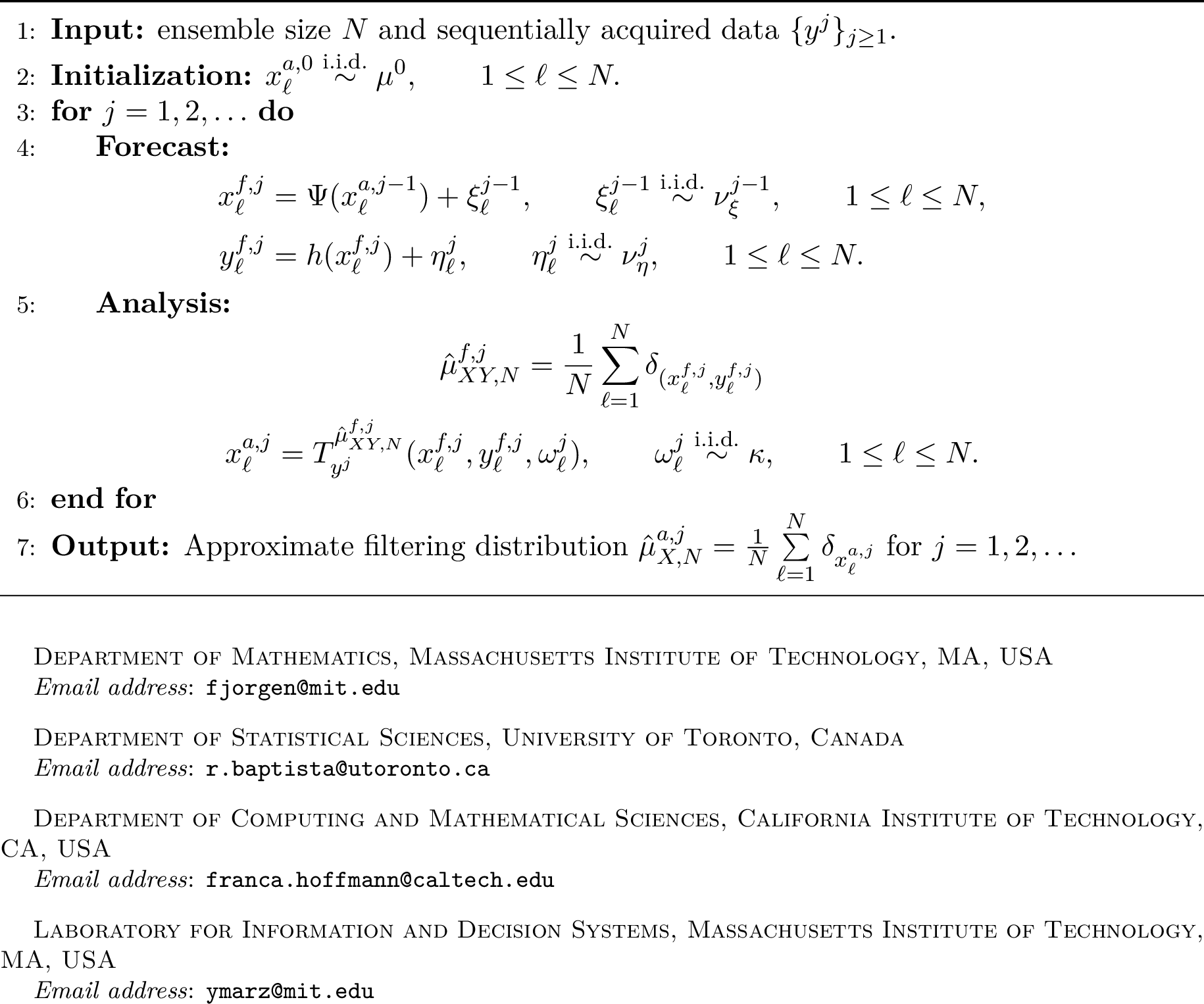
In practice, the transport map is usually constructed from the empirical joint forecast \(\hat{\mu}_{XY,N}^{f,j}\) and the new observation \(y^j\). Then, the analysis particles are obtained by evaluating the map at each sample from the forecast distribution in Equation 11 . That is, \[\label{eq:particle95stochastic95updates} x_{\ell}^{a,j}= T^{\hat{\mu}^{f, j}_{XY,N}}_{y^j} \bigl ( x_{\ell}^{f,j}, y_{\ell}^{f,j}, \omega_\ell^j \bigr), \quad \omega_\ell^{j} \overset{\text{i.i.d.}}{\sim} \kappa, \qquad \ell = 1,\dots,N.\tag{13}\] Consequently, the \(x_{\ell}^{a,j}\) are generally not i.i.d.; they interact through their common dependence on the forecast \(\hat{\mu}_{XY,N}^{f,j}\). Equation 13 completes the recursion for \(\hat{\mu}_{X,N}^{a,j}\) in time and yields a fully specified filtering algorithm via Equations 9 , 10 , 11 , and 13 . We summarize this scheme in Algorithm 1 and call this class of algorithms transport ensemble filters. The term transport ensemble filters should not be confused with ensemble transform Kalman filters [12], [13], or with more general ensemble transform methods and particle filters based on optimal transport [1], [14], [15]. In our terminology, transport refers broadly to the particle-wise analysis map in Algorithm 1; in this sense, ensemble transport filters [16] can be viewed as falling under our template, whereas the cited optimal-transport particle filters and ensemble transform Kalman filters are distinct notions and are not meant to be included here.
This work addresses the central question of consistency of transport ensemble filtering algorithms: what is the limiting behavior of the empirical measure \(\hat{\mu}_{X,N}^{a,j}\) generated by the interacting particle scheme in Equation 13 , and how is it related to the true filtering distribution \(\mu_X^{a,j}\) for each time \(j\)? Intuitively, under mild regularity of \(T\), increasing \(N\) weakens the interaction among particles through the forecast \(\hat{\mu}_{XY,N}^{f,j}\), suggesting convergence as \(N\to\infty\). This phenomenon—particles becoming asymptotically independent—is known as propagation of chaos [17], [18]. The main objective of this paper is to make this intuition precise and to answer the following two questions:
What is the mean-field law \(\tilde{\mu}_X^{a,j}\) to which \(\hat{\mu}_{X,N}^{a,j}\) converges in a suitable sense as the number of particles grows \(N\rightarrow \infty\)?
At what rate does \(\hat{\mu}_{X,N}^{a,j}\) converge to the mean-field law \(\tilde{\mu}_X^{a,j}\)?
Remark 1. We work on \(\mathcal{P}_2(\mathbb{R}^{n}\times\mathbb{R}^{m})\) for two reasons. First, most linear and nonlinear transport ensemble filters (e.g., EnKF, EnSMF, CMF) are formulated at least in terms of first- and second-order moments (e.g., means, covariances, and/or covariances of nonlinear features). Second, \(\mathcal{P}_2\) equips the space with the 2-Wasserstein distance \(W_2\), which provides a geometric and statistically meaningful metric for both (i) assessing prediction error of the empirical law \(\hat{\mu}_{X,N}^{a,j}\) and (ii) analyzing empirical measures.
1.2 Related Work↩︎
To the best of our knowledge, there are no results establishing mean-field convergence bounds for nonlinear transport ensemble filters—i.e., when the analysis step is implemented via a nonlinear map \(T^\pi_{y^j}\) in Equation 13 —as in, for example, the EnSMF or CMF [8], [9].
By contrast, for the specific case of EnKF-type algorithms in which \(T^\pi_{y^j}\) is an affine map, some results are available in the literature. The earliest mean-field convergence results for the EnKF are due to Mandel et al. [19] and Le Gland et al. [20]. In the linear-Gaussian setting (linear \(\Psi\), linear \(h\), and Gaussian noise/initialization in Equation 1 ), Mandel et al.prove convergence of the first two moments of the empirical analysis ensemble \(\hat{\mu}_{X,N}^{a,j}\) as \(N\to\infty\). Thus, in expectation over the particle draws of \((\xi_\ell^{j-1}, \eta_\ell^{j})\), the ensemble statistics of \(\hat{\mu}_{X,N}^{a,j}\) converge in \(L^{p}\), for all \(p\in[1,\infty)\), to those of the mean-field \(\tilde{\mu}_X^{a,j}\) (which coincides with \(\mu_X^{a,j}\) in the linear-Gaussian setting). Le Gland et al.extend this line of analysis: for Gaussian noise variables, initial condition \(\mu^0\) with bounded moments of all orders, locally Lipschitz \(\Psi\), and linear \(h\) in Equation 1 , the authors identify the mean-field limit \(\tilde{\mu}_X^{a,j}\) and show that, for locally Lipschitz test functions with polynomial growth at infinity \(\varphi:\mathbb{R}^n\to\mathbb{R}\), we have \[\label{eq:previous95work95bound} \left(\mathbb{E}\Bigl|\textstyle\int \varphi \, \mathrm{d}\hat{\mu}_{X,N}^{a,j}-\int \varphi \, \mathrm{d}\tilde{\mu}_{X}^{a,j}\Bigr|^p\right)^{1/p} =O\left(N^{-1/2}\right)\tag{14}\] for any \(p \geq 1\). A more concise proof, with explicit dependence of the \(O(N^{-1/2})\) constant on the relevant moments, is given in the recent work of Calvello et al. [21]. Law et al. [22] restate the result in Equation 14 and broaden the class of admissible test functions \(\varphi\) to include bounded functions as well. For the ensemble square root filter (ESRF), Kwiatkowski and Mandel [23] obtain analogous mean-field convergence using similar techniques, and the recent work of Al-Ghattas and Sanz-Alonso [24] proves the first dimension-independent and non-asymptotic \(O\left(N^{-1/2}\right)\) convergence rates of the first two moments for the first ESRF update (i.e., at time \(j = 1\)) in the linear-Gaussian setting. A related but distinct thread studies state-estimation accuracy of EnKF-type algorithms (rather than convergence of empirical measures), typically under dissipativity of the dynamics, linear and sufficiently informative observation operators, Gaussian noise variables, and Gaussian initial condition. Representative results include well-posedness and estimation accuracy for the perturbed-observation EnKF [25], accuracy and stability of localized variants (based on sparse regularization of the covariances in the EnKF map) [26], [27], and long-time/stability analyses under structural assumptions on the dynamics and observations [28].
There is also a parallel literature on the continuous-time limit of filtering, often called the ensemble Kalman–Bucy filter (EnKBF). These works use techniques different from the discrete-time setting to establish mean-field limits, stability, and propagation-of-chaos-type results for the associated McKean–Vlasov dynamics; see, e.g., Del Moral and coauthors [29], [30], de Wiljes et al. [31], and recent overviews such as Bishop and Del Moral [32].
1.3 Main Results↩︎
Our results advance the theory of ensemble filtering by developing a unified mean-field convergence framework for the broad class of transport ensemble filters defined in Algorithm 1. This framework includes the EnKF as a special case, thereby furthering EnKF theory, while allowing for genuinely nonlinear analysis maps, such as the EnSMF [8]. For transports in this broad class, we identify the mean-field limit \(\tilde{\mu}^{a,j}_{X}\) in Equation 20 . Our main technical result in Theorem 1 proves convergence of the algorithmic ensemble \(\hat{\mu}^{a,j}_{X,N}\) to this mean-field limit. More precisely, we construct a coupling of the interacting analysis ensemble \(\hat{\mu}_{X,N}^{a,j}\) with an empirical measure \(\tilde{\mu}_{X,N}^{a,j}\) of i.i.d.mean-field particles such that for a finite time horizon \(J\in\mathbb{N}\) we have the pathwise convergence \[\label{eq:informal951} \sup_{1 \leq j \leq J}W_2\bigl(\hat{\mu}_{X,N}^{a,j},\tilde{\mu}_{X, N}^{a,j}\bigr) \lesssim N^{-1/2},\tag{15}\] with high probability (Theorem 1) and in expectation (Corollary 1). In both results, the probability and expectation are taken over both the particle draws in Algorithm 1 and the observation realizations \(y^{1:j}\).
Remark 2. Our proofs also imply that with high probability we have the pathwise bound \[\sup_{1 \leq j \leq J}\sqrt{\frac{1}{N}\sum\limits_{\ell = 1}^N \left\|x_{\ell}^{a,j} - v_\ell^{a,j}\right\|_2^2}\lesssim N^{-1/2},\] where \(v_\ell^{a,j}\) are mean-field i.i.d.particles. This is a tighter bound and closer to the classical way of stating propagation of chaos results in the literature [18], [33]. We will state our results by comparing measures, i.e., in the form of Equation 15 , for ease of presentation.
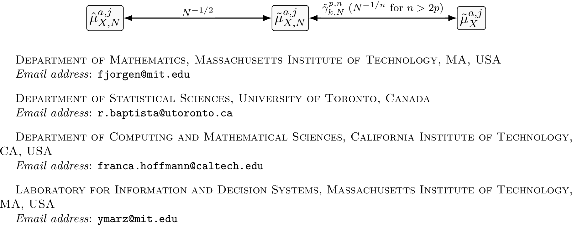
Our results show that the interacting particle system is quantitatively close to an i.i.d.sample from the mean-field law at the \(N^{-1/2}\) rate. For a confidence parameter \(k\ge2\), corresponding to events of probability at least \(1-1/k\), the component of the standard i.i.d.Wasserstein convergence rate [34], [35] is \[\label{eq:standard95iid95wasserstein95rate} \gamma_{k,N}^{p,n} = \begin{cases} \left(\frac{\log k}{N}\right)^{1/n} &\text{if } 1\le p < \frac{n}{2},\\ \left(\frac{\log k}{N}\right)^{1/n}\bigl(\log(2+N)\bigr)^{2/n} &\text{if } p = \frac{n}{2},\\ \left(\frac{\log k}{N}\right)^{1/(2p)} &\text{if } \frac{n}{2} < p \le 2. \end{cases}\tag{16}\] Combining Equation 15 with the rate in Equation 16 yields a convergence result \[\label{eq:informal952} \sup_{1 \leq j \leq J}W_p\bigl(\hat{\mu}_{X,N}^{a,j},\tilde{\mu}_{X}^{a,j}\bigr) \lesssim \gamma_{k,N}^{p,n}+\frac{(\log k)^{1+J/2}}{\sqrt N}.\tag{17}\] This bound holds with probability \(1-1/k\) over the particle realizations and observations for \(1 \le p \le 2\). In the high-dimensional regime \(n>2p\), the empirical-measure term reduces to \(N^{-1/n}\) and dominates the Monte Carlo interaction term for fixed \(k\) and \(J\). We state the result formally in Corollary 2.
The main ideas and the full proofs of our results are developed in Sections 2 and 3. Our proofs rely on a classical synchronous coupling argument, by driving \(\hat{\mu}_{X,N}^{a,j}\) and \(\tilde{\mu}_{X, N}^{a,j}\) with the same noise (Subsection 2.2), and the main technical challenge lies in handling the moments of the intermediate distributions (Subsections 3.3 and 3.4) as well as their dependence on the random observations \(y^{1:j}\) (Subsections 3.2 and 3.3). In the process, we derive an interesting technical result in Proposition 5 on the high-probability stability of sub-Gaussianity under disintegration and conditioning. In order to prove this result, we introduce an equivalent characterization of sub-Gaussianity that extends the moment-generating-function definition to non-centered random variables.
Section 4 presents applications of the results derived in the earlier sections to specific transport ensemble filters. Subsections 4.1 and 4.2 illustrate how Equations 15 and 17 specialize to the EnKF and to the nonlinear transport analogue, the EnSMF, respectively. In the EnKF case, these results improve the convergence analyses in [20], [19], and [23] along several axes: first, our statements account for the randomness of the observation path, rather than conditioning on a fixed \(y^{1:J}\). Second, we control (with high probability) the observational and algorithmic randomness, rather than only obtaining convergence in expectation. Third, our bounds are stated in Wasserstein metrics on \(\mathcal{P}_2( \mathbb{R}^n)\) (as opposed to single test-function averages), thereby directly quantifying distributional error. Fourth, we allow more general noise variables (i.e., sub-Gaussian, as opposed to Gaussian). Fifth, we replace the linear observation assumption by a Lipschitz condition on \(h\), accommodating nonlinear observation operators. Finally, our guarantees are non-asymptotic in \(N\), delivering the first explicit finite-sample rates, whereas all previous results for the EnKF held in the asymptotic regime.
Remark 3. Another way to relate these results to bounds of the form in Equation 14 appearing in the literature is as follows. Since the \(W_p\) distance for \(p\ge 1\) dominates the \(W_1\) distance, and \(W_1\) admits a variational characterization in terms of Lipschitz functions \(\varphi\) with constant \(\mathrm{Lip}(\varphi)\), it follows from Equations 15 and 17 that the following uniform convergence bounds hold: \[\begin{align} \sup_{1 \le j \le J} \sup_{\mathrm{Lip}(\varphi)\le 1} \Bigl|\textstyle\int \varphi \, \mathrm{d}\hat{\mu}_{X,N}^{a,j}-\int \varphi \, \mathrm{d}\tilde{\mu}_{X, N}^{a,j}\Bigr| &\lesssim N^{-1/2}\\ \sup_{1 \le j \le J} \sup_{\mathrm{Lip}(\varphi)\le 1} \Bigl|\textstyle\int \varphi \, \mathrm{d}\hat{\mu}_{X,N}^{a,j}-\int \varphi \, \mathrm{d}\tilde{\mu}_{X}^{a,j}\Bigr| &\lesssim \gamma_{k,N}^{p,n} +\frac{(\log k)^{1+J/2}}{\sqrt N}, \end{align}\] where \(\mathrm{Lip}(\varphi)\) denotes the Lipschitz constant of \(\varphi\). The first bound holds both with high probability and in expectation. The second one holds with high probability as displayed, and in expectation with \(\gamma_{k,N}^{p,n}\) replaced by a \(k\)-independent factor \(\bar\gamma_N^{p,n}\).
1.4 Notation and Basic Definitions↩︎
Throughout the paper we use the conventions \(\mathbb{N}=\{0,1,2,\ldots\}\) and \(\mathbb{N}_{\ge 1}=\{1,2,\ldots\}\). Moreover, we work on finite-dimensional Euclidean spaces: vectors are equipped with the Euclidean norm \(\|x\|_{2}\) and matrices with the induced operator norm \(\left\|A\right\|_{2}=\sup_{\|x\|_{2}=1}\|Ax\|_{2}\). All Lipschitz constants are taken with respect to these norms. The Moore–Penrose pseudoinverse of a matrix \(A\) is denoted by \(A^{\dagger}\). For \(u \in \mathbb{N}_{\ge 1}\), the identity map on \(\mathbb{R}^{u}\) is \(I_{u}\); more generally \(I_{V}\) denotes the identity on a vector space \(V\). For any Lipschitz function \(f\) between Euclidean vector spaces, we define \(\mathrm{Lip}(f)\) as the smallest Lipschitz constant of \(f\). For \(x \in \mathbb{R}^u\) and any integer \(1 \le k \le u\), we define the subvector \(x_{1:k} = (x_1,x_2,\dots,x_k) \in\mathbb{R}^k\). For a sequence of vectors \(y^j \in \mathbb{R}^d\), \(d\in \mathbb{N}_{\geq 1}\) we write \(y^{1:J}=(y^{1},\dots,y^{J})\in(\mathbb{R}^{d})^{J}\). All probability measures are defined on the Borel \(\sigma\)-algebra \(\mathcal{B}(\mathbb{R}^{u})\) of the relevant space. We use \(\mathcal{P}(\mathbb{R}^{u})\) for all Borel probability measures on \(\mathbb{R}^{u}\) and consider the subset of measures \[\begin{align} \mathcal{P}_{p}(\mathbb{R}^{u}) &=\Bigl\{\mu\in\mathcal{P}(\mathbb{R}^{u}) : \int\|x\|_{2}^{p} \, \mathrm{d}\mu(x)<\infty\Bigr\}. \end{align}\] A real random variable \(X\) is sub-Gaussian with parameter \(K\) (cf. Def. 2.5.5 of [36]) if there exists \(K>0\) such that \[\mathbb{E}\bigl(e^{X^2/K^2}\bigr)\le2.\] Equivalently, by introducing the \(\psi_2\)-Orlicz norm \[\label{eq:Orlicz} \|X\|_{\psi_2} := \inf\Bigl\{t>0 : \mathbb{E}\bigl(e^{(X/t)^2}\bigr)\le2\Bigr\},\tag{18}\] we have that \(X\) is sub-Gaussian when \(\|X\|_{\psi_2}<\infty\). Note that the infimum in 18 is attained unless \(X\) is almost surely \(0\). We extend the definition to probability measures through \(\|\mu\|_{\psi_2} = \|X\|_{\psi_2}\) for \(X \sim \mu\). The notion generalizes directly to vectors (cf. [36]): a random vector \(X\in\mathbb{R}^u\) is sub-Gaussian if \[\|X\|_{\psi_2} \mathrel{\vcenter{:}}= \sup_{\|v\|_2=1}\|v^\top X\|_{\psi_2} <\infty.\] To take the sub-Gaussian norm of the Euclidean norm of a random vector we will write \[\|X\|_{2,\psi_2} \mathrel{\vcenter{:}}= \left\|\|X\|_2\right\|_{\psi_2},\] instead, and similarly for measures \(\mu \in \mathcal{P}(\mathbb{R}^u)\), we write \(\|\mu\|_{2,\psi_2} = \|X\|_{2,\psi_2}\) for \(X\sim \mu\). We fix dimensions \(n,m\in\mathbb{N}_{\ge1}\) corresponding to the state and observation spaces \(\mathbb{R}^{n}\) and \(\mathbb{R}^{m}\), respectively. For a joint law \(\mu\in\mathcal{P}\!\bigl(\mathbb{R}^{n}\times\mathbb{R}^{m}\bigr)\), we define the coordinate projections \[\operatorname{pr}_X:\mathbb{R}^{n}\times\mathbb{R}^{m}\to\mathbb{R}^{n},\quad\operatorname{pr}_X(x,y)=x, \qquad \operatorname{pr}_Y:\mathbb{R}^{n}\times\mathbb{R}^{m}\to\mathbb{R}^{m},\quad\operatorname{pr}_Y(x,y)=y.\] The \(X\)-marginal and \(Y\)-marginal of \(\mu\) are given by the pushforward distributions \[\mu_X \mathrel{\vcenter{:}}= (\operatorname{pr}_X)_{\sharp}\mu, \qquad \mu_Y \mathrel{\vcenter{:}}= (\operatorname{pr}_Y)_{\sharp}\mu.\] Moreover, we write \(\mu_{XY}=\mu\) for the full joint distribution. Because \(\mathbb{R}^{n}\) and \(\mathbb{R}^{m}\) are Polish spaces (hence standard Borel), the disintegration theorem (e.g., [37]) ensures the existence of a regular conditional probability measure given by the map \[y \mapsto \mu_{X\mid Y=y}\in\mathcal{P}(\mathbb{R}^{n}),\] satisfying \[\mu(A\times B)=\int_{B}\mu_{X\mid Y=y}(A) \, \mathrm{d}\mu_{Y}(y), \qquad \forall A\in\mathcal{B}(\mathbb{R}^{n}),B\in\mathcal{B}(\mathbb{R}^{m}),\] where \(y\mapsto\mu_{X\mid Y=y}(A)\) is Borel-measurable for every fixed \(A\). We call \(\mu_{X\mid Y=y}\) the conditional distribution of \(X\) given \(Y=y\); the map \(y\mapsto\mu_{X\mid Y=y}\) is unique \(\mu_{Y}\)-a.s. For random vectors \(X\in\mathbb{R}^{u_1}\) and \(Y\in\mathbb{R}^{u_2}\) we write \(\mathbb{E}(X)\) for expectation, \[\mathrm{Cov}(X,Y) \mathrel{\vcenter{:}}= \mathbb{E}\,\!\bigl((X-\mathbb{E}X)(Y-\mathbb{E}Y)^{\mathsf T}\bigr) \in\mathbb{R}^{u_1\times u_2},\] for the cross-covariance matrix of \(X\) and \(Y\) (if it exists), and \(\mathrm{Cov}(X) \mathrel{\vcenter{:}}= \mathrm{Cov}(X,X)\) for the covariance matrix. In particular, note that \(\mathrm{Cov}((X,Y)) \in \mathbb{R}^{(u_1+u_2)\times(u_1+u_2)}\) is the covariance of the random variable \((X,Y)\). \(\mathrm{Law}(X)\) is the distribution of \(X\), the trace of a matrix is \(\text{Tr}(\cdot)\), and we abbreviate \(\text{Tr}\mathrm{Cov}(X)\mathrel{\vcenter{:}}= \text{Tr}\bigl(\mathrm{Cov}(X)\bigr).\) For \(\mu\in\mathcal{P}_1(\mathbb{R}^u)\), we write \(\mathbb{E}\mu\) for its mean and define the centered measure \[\mu-\mathbb{E}\mu \mathrel{\vcenter{:}}= (x\mapsto x-\mathbb{E}\mu)_\sharp\mu.\] Similarly, \(\|\mu-\mathbb{E}\mu\|_{2,\psi_2}\) means \(\|X-\mathbb{E}X\|_{2,\psi_2}\) and \(\|\mu\|_{2,\psi_2}\) means \(\|X\|_{2,\psi_2}\) for any \(X\sim\mu\), when finite. For \(\mu\in\mathcal{P}_2(\mathbb{R}^u)\), covariance-related quantities are defined by considering \(X\sim\mu\); in particular, \(\mathrm{Cov}(\mu)\mathrel{\vcenter{:}}=\mathrm{Cov}(X)\) and \(\text{Tr}\mathrm{Cov}(\mu)\mathrel{\vcenter{:}}=\text{Tr}(\mathrm{Cov}(\mu))\). If the displayed Orlicz norm is finite, then \(\text{Tr}\mathrm{Cov}(\mu)\le 2 \|\mu-\mathbb{E}\mu\|_{2,\psi_2}^2\le 8 \|\mu\|_{2,\psi_2}^2\). For \(\mu\in\mathcal{P}_{q}(\mathbb{R}^{u})\) and \(q\ge1\) we use the centered \(q\)-th moment \[\overline{M}_{q}(\mu)= \Bigl(\int\|x-\mathbb{E}\mu\|_{2}^{q}\,\mathrm{d}\mu(x)\Bigr)^{1/q}.\] For \(\mu,\nu\in\mathcal{P}_{p}(\mathbb{R}^{u})\) (\(p\ge1\)), the \(p\)-Wasserstein distance is \[W_{p}(\mu,\nu)= \Bigl(\inf_{\pi\in\Pi(\mu,\nu)}\int\|x-y\|_{2}^{p} \, \mathrm{d}\pi(x,y)\Bigr)^{1/p},\] where \(\Pi(\mu,\nu)\) is the set of couplings with marginals \(\mu,\nu\). Tildes denote mean-field quantities, hats denote interacting empirical measures, and a subscript \(N\) denotes an empirical measure.
2 Mean-Field Approximation and Proof Strategy↩︎
2.1 Deriving Mean-Field Dynamics↩︎
In the transport ensemble filter, the particles are coupled through the update map \(T\): each particle’s position after the analysis step depends not only on its own forecast position \((x_{\ell}^{f,j},y_{\ell}^{f,j})\) but also on the empirical joint forecast distribution \(\hat{\mu}_{XY,N}^{f,j}\). This creates an \(N\)-particle interacting system. The mean-field approximation is a standard way to handle such models: instead of tracking all interactions explicitly, we approximate the random empirical laws \(\hat{\mu}_{XY,N}^{f,j}\) and \(\hat{\mu}_{X,N}^{a,j}\) with deterministic measures \(\tilde{\mu}_{XY}^{f,j}\) and \(\tilde{\mu}_{X}^{a,j}\) (given \(y^{1:j}\)) in the regime where \(N\) becomes infinite. In this infinite-ensemble limit, particles become independent with common law, and their interaction through \(T\) is replaced by the response to a fixed mean-field. To make this idea more concrete, consider a representative mean-field particle \(U^{j-1}\sim \tilde{\mu}_X^{a,j-1}\). By drawing fresh noise, \[\xi^{j-1}\sim \nu_\xi^{j-1}, \qquad \eta^{j}\sim \nu_\eta^{j},\] the forecast step in the mean field stays the same, i.e., \[(U^{f,j},Y^{f,j}) =\Bigl(\Psi(U^{j-1})+\xi^{j-1}, \, h(\Psi(U^{j-1})+\xi^{j-1})+\eta^{j}\Bigr),\] in law or, equivalently, \[\tilde{\mu}_{XY}^{f,j} =Q^jP^{j-1} \tilde{\mu}_{X}^{a,j-1}.\] For the analysis step in Equation 13 , however, we replace the random empirical law by the deterministic forecast law \(\tilde{\mu}_{XY}^{f,j}\). This means that the mean-field particle is updated using the map \[U^{j} =T_{y^j}^{\tilde{\mu}_{XY}^{f,j}}\!\bigl(U^{f,j},Y^{f,j},\omega^{j}\bigr),\] where \(\omega^{j}\sim \kappa\) is an independent auxiliary random sample and we assume that the expression above is well-defined (i.e., \(\tilde{\mu}_{XY}^{f,j}\in\mathcal{P}_2\left(\mathbb{R}^n\times\mathbb{R}^m\right)\); we will verify this under sufficient regularity of Equation 1 in the next section). We define the mean-field approximate conditioning operator given \(\nu \in \mathcal{P}_2\left(\mathbb{R}^n\times\mathbb{R}^m \right)\), whenever the following pushforward lies in \(\mathcal{P}_2(\mathbb{R}^n)\) (as will be ensured under the conditions established in the next section), as \[\label{eq:mean95field95operator} \tilde{B}_{y^j}^\nu:\mathcal{P}_2(\mathbb{R}^{n}\times \mathbb{R}^{m})\to \mathcal{P}_2(\mathbb{R}^n), \qquad \tilde{B}_{y^j}^\nu\pi\mathrel{\vcenter{:}}= \bigl(T_{y^j}^\nu\bigr)_\sharp\!\bigl(\pi\otimes \kappa\bigr),\tag{19}\] with the abbreviation \(\tilde{B}_{y^j} \pi\mathrel{\vcenter{:}}= \tilde{B}_{y^j}^\pi\pi\). Using \(\tilde{B}\), we rewrite the update on the law of \(U^{j}\) as \[\tilde{\mu}_X^{a,j}=\mathrm{Law}(U^{j}) = \tilde{B}_{y^j}\tilde{\mu}_{XY}^{f,j}.\] Then, collecting both steps from above, the derived limiting mean-field system is \[\label{eq:mf95alg95measure95perspective} \begin{align} \tilde{\mu}_X^{a,0} &= \mu^0,\\ \tilde{\mu}_X^{a,j} &= \tilde{B}_{y^j} Q^j P^{j-1}\tilde{\mu}_X^{a,j-1}. \end{align}\tag{20}\] This recursion mirrors the exact filtering recursion in Equation 8 , with \(B_{y^j}\) replaced by the approximate conditioning operator \(\tilde{B}_{y^j}\) defined through \(T\). The argument above is heuristic, and we will prove formally that \(\hat{\mu}_{X,N}^{a,j}\) converges to the mean-field system \(\tilde{\mu}^{a,j}_{X}\) in the next sections.
2.2 Idea of the Proof↩︎
Our goal is to show that the interacting particle system \(\hat{\mu}_{X,N}^{a,j}\) converges to the mean-field system \(\tilde{\mu}^{a,j}_{X}\) in \(W_p\)-distance. To prove this, we apply the classic idea of a synchronous coupling [18], [38]: we construct an i.i.d.mean-field ensemble of size \(N\), \((v_\ell^{a,j})_{\ell=1}^N\), whose empirical laws \((\tilde{\mu}^{f,j}_{XY,N},\tilde{\mu}^{a,j}_{X,N})\) are sampled from the mean-field recursion. When the observation path is random, this i.i.d.statement is understood conditional on that path; for readability, we omit this qualifier below. The key idea is to couple \((\tilde{\mu}^{f,j}_{XY,N},\tilde{\mu}^{a,j}_{X,N})\) and \((\hat{\mu}^{f,j}_{XY,N},\hat{\mu}^{a,j}_{X,N})\) by driving them with the same randomness \(\{(\xi_\ell^{j-1},\eta_\ell^j,\omega_\ell^j)\}_{\ell=1}^N\) at every step \(j\). This ensures that any discrepancy stems only from the interaction caused by the dependence of \(T\) on the empirical forecast distribution \(\hat{\mu}_{XY,N}^{f,j}\), which we will refer to as an interaction term. This allows us to make an inductive argument. For fixed \(N\) and for each \(j\), we draw i.i.d.initializations \(\{x_{\ell}^{a,0}\}_{\ell=1}^N \sim \mu^0\) and i.i.d.noise samples \(\{(\xi_\ell^{j-1},\eta_\ell^{j},\omega_\ell^{j})\}_{\ell=1}^N \sim \nu_\xi^{j-1}\!\otimes\!\nu_\eta^{j}\!\otimes\!\kappa\), independent across \(j\). Then, we define the coupling as follows, letting \(v_\ell^{a,0} = x_{\ell}^{a,0}\): \[\tag{21} \begin{figure}\includegraphics[width=0.8\textwidth]{_pdflatex/euljhbwf.png}\tag{22}\end{figure}\hfill \begin{figure}\includegraphics[width=0.8\textwidth]{_pdflatex/tzhaonsj.png}\tag{23}\end{figure}\] To compare \(\tilde{\mu}_{X,N}^{a,j}\) to the mean-field distribution \(\tilde{\mu}_{X}^{a,j}\) defined in Equation 20 , it is instructive to apply the triangle inequality \[\label{eq:triangle95intuitive951} W_p(\hat{\mu}^{a,j}_{X,N},\tilde{\mu}^{a,j}_{X}) \leq W_p(\hat{\mu}^{a,j}_{X,N},\tilde{\mu}^{a,j}_{X, N}) +W_p(\tilde{\mu}^{a,j}_{X, N},\tilde{\mu}^{a,j}_{X}).\tag{24}\] Since \(\tilde{\mu}^{a,j}_{X, N}\) consists of i.i.d.particles, the second term \(W_p(\tilde{\mu}^{a,j}_{X, N},\tilde{\mu}^{a,j}_{X})\) can be explicitly controlled in expectation or with high probability, non-recursively, through a rate \(\gamma(N)\) using modern Wasserstein convergence results [35], as long as we can control higher moments of \(\tilde{\mu}^{a,j}_{X}\). \(\gamma(N)\) typically suffers from the curse of dimensionality: for \(p\)-Wasserstein distances in \(\mathbb{R}^n\), it scales as \(\gamma(N)\asymp N^{-1/n}\), which is known to be sharp in general [35]. For this reason, simply controlling \(W_p(\hat{\mu}^{a,j}_{X,N},\tilde{\mu}^{a,j}_{X})\) conflates the interaction error with the slow i.i.d.sampling rate \(W_p(\tilde{\mu}^{a,j}_{X,N},\tilde{\mu}^{a,j}_{X})\) in high dimensions.
As a result, it is informative to separate the scale of the second term in the upper bound in Equation 24 and to study the first term \(W_p(\hat{\mu}^{a,j}_{X,N},\tilde{\mu}^{a,j}_{X,N})\) in isolation: it captures the algorithmic interaction error by quantifying how close the interacting ensemble is to behaving like an i.i.d.sample from the mean-field law. Given sufficient Lipschitz regularity of \(T\) (Assumption 2) and the dynamics model (Assumption 1), we will show that it satisfies a self-recursion \[\label{eq:triangle95intuitive952} W_p(\hat{\mu}^{a,j}_{X,N},\tilde{\mu}^{a,j}_{X, N}) \leq C_1W_p(\hat{\mu}^{a,j-1}_{X,N},\tilde{\mu}^{a,j-1}_{X, N}) + C_2/\sqrt{N},\tag{25}\] where \(C_1\) and \(C_2\) are random variables. The second term enters this upper bound because of the discrepancy caused by the interaction measure in \(T\) between \(\hat{\mu}^{a,j}_{X,N}\) and \(\tilde{\mu}^{a,j}_{X, N}\). Then, Equation 25 yields an inductive bound \(W_p(\hat{\mu}^{a,j}_{X,N},\tilde{\mu}^{a,j}_{X,N})\lesssim N^{-1/2}\) with high probability and in expectation, and this is essentially the proof of the main result (Theorem 1). As a direct corollary, we obtain the corresponding high-probability and expectation bounds for \(W_p(\hat{\mu}^{a,j}_{X,N},\tilde{\mu}^{a,j}_{X})\) using the empirical-measure rates in Corollary 2. The key ingredient in these proofs is to obtain high-probability bounds on the random variables \(C_1\) and \(C_2\) in Equation 25 . To obtain such bounds, we need to control the moments and tails of the distributions \(\mu^{f,j}_{XY}\), \(\hat{\mu}^{f,j}_{XY,N}\), \(\tilde{\mu}^{f,j}_{XY,N}\), and \(\tilde{\mu}^{f,j}_{XY}\) as well as some of their differences (with high probability for the random empirical measures).
Before formulating these bounds, we make explicit one additional source of randomness: all the measures we defined (e.g., \(\hat{\mu}_{X,N}^{a,j}\), \(\tilde{\mu}_{X}^{a,j}\), \(\mu^{a,j}_{X}\)) depend implicitly on the observation path \(y^{1:j}\). Under the model in Equation 1 , however, the observation sequence \(Y^{1:j}\) itself is random, and this randomness should be taken into account when formulating the bounds with high probability or in expectation. Letting \(J\in\mathbb{N}\) be a finite time horizon and using the stochastic process \(Y^{1:j}\) given by Equation 1 , we define \[\label{eq:rho95def} \rho^J \mathrel{\vcenter{:}}= \mathrm{Law}(Y^{1:J}),\tag{26}\] and promote \(y^{1:J}\) to a random draw \(Y^{1:J}\sim\rho^J\). This observation path is taken independent of the algorithmic particle, noise, and auxiliary variables used to construct the interacting and mean-field ensembles. Henceforth, all bounds will be stated in probability or in expectation with respect to this joint law.
3 Proving Convergence to the Mean-Field↩︎
In this section, we will present and prove our main result, Theorem 1 (Subsection 3.1). The argument hinges on three ingredients: (i) high-probability control of moments of the forecast distribution under random observations (Subsection 3.2), (ii) analogous moment bounds for the mean-field dynamics (Subsection 3.3), and (iii) concentration of empirical moments for the interacting system (Subsection 3.4). After building up these technical preliminaries, we combine them to prove Theorem 1 in Subsection 3.5.
3.1 Mean-Field Limit Statements↩︎
The main result of this section is the control of the distance between the interacting particles and the i.i.d.draws from the corresponding mean-field distribution as defined in Equation 21 . This result holds under Assumptions 1 and 2, which are introduced in the following sections.
Theorem 1. Fix \(J\in\mathbb{N}_{\ge1}\), draw \(Y^{1:J} \sim \rho^J\), and suppose Assumptions 1 and 2 hold. Let \(\{\hat{\mu}_{X,N}^{a,j}\}_{j=1}^{J}\) be the analysis empirical measures generated by the interacting-particle system and \(\{\tilde{\mu}_{X, N}^{a,j}\}_{j=1}^{J}\) the corresponding i.i.d.mean-field sequence as coupled in Equation 21 , both using observations \(y^{1:J}=Y^{1:J}\). Then there exists a constant \(C\mathrel{\vcenter{:}}= C(\mathcal{Q})>0\) depending only on the quantities \[\mathcal{Q} \mathrel{\vcenter{:}}= (n,m,a,b,\sigma_{\max},\lambda_{\max},\sigma_X, L_\Psi,L_h,C_{\mathrm{L}},L_y,e_{\mathrm{L}}, C_{\mathrm{est}},e_{\mathrm{est},1},e_{\mathrm{est},2},e_y, \sigma_\kappa,J,L_g)\] such that for all \(k\ge 2\), with probability at least \(1-\frac{1}{k}\), \[W_2\bigl(\hat{\mu}_{X,N}^{a,j},\tilde{\mu}_{X, N}^{a,j}\bigr)\leq C \left(1 + \left( \frac{\log k}{\sqrt{N}}\right)^{p_j}\right)\frac{(\log k)^{1 + j/2}}{\sqrt{N}} \text{ for all } 1 \leq j \leq J,\] where \(p_j \mathrel{\vcenter{:}}=(1+2e_\mathrm{L})^{J-1}\left(e_{\mathrm{est},1} + (j-1)\max\left(e_\mathrm{L}, e_{\mathrm{est},1} +\frac{1}{2}\right)\right)\). In particular, if \(N\geq (\log k)^2\), \[\sup_{1 \leq j \leq J}W_2\bigl(\hat{\mu}_{X,N}^{a,j},\tilde{\mu}_{X, N}^{a,j}\bigr)\leq C\frac{(\log k)^{1 +J/2}}{\sqrt{N}},\] with the same probability. The randomness in the expression \(W_2\bigl(\hat{\mu}_{X,N}^{a,j},\tilde{\mu}_{X, N}^{a,j}\bigr)\) is over particle realizations and over the assumed values of the observations \(Y^{1:J}\).
Remark 4. The constant \(C(\mathcal{Q})\) diverges to infinity as \(J\to\infty\) and thus the bounds in Theorem 1 only hold for finite time. Extending these bounds to infinite time horizons is of key interest for the analysis of filtering algorithms.
As an immediate corollary, through the elementary equality for non-negative scalar random variables \(X\) with finite expectation \(\mathbb{E}(X) = \int_0^{\infty} \mathbb{P}(X > t)dt\), we can bound the expectation over particle realizations and observations.
Corollary 1. Consider the same setting as in Theorem 1. Then, \[\mathbb{E}\left(\sup_{1 \leq j \leq J}W_2 \bigl(\hat{\mu}_{X,N}^{a,j},\tilde{\mu}_{X, N}^{a,j}\bigr)\right) \;\le\; \frac{C'(\mathcal{Q})}{\sqrt{N}}\] with a constant \(C' \mathrel{\vcenter{:}}= C'(\mathcal{Q})>0\).
Remark 5. Note that sub-Gaussian tail assumptions are only needed for the high–probability statements in Theorem 1. For the bound in Corollary 1 it would also suffice to assume moment control of the driving noises and the initialization in Assumptions 1 and 2.
Next, we would like to bound \(W_p\bigl(\hat{\mu}_{X,N}^{a,j},\tilde{\mu}_X^{a,j}\bigr)\) for \(1\le p \le 2\), for which we use the concentration result Proposition 9 in Appendix 5.1 following Example 3.4 of [34] (we also refer to Theorem 2 of [35]). We use the high-probability empirical-measure rate \(\tilde{\gamma}_{k,N}^{p,d}\) defined in Proposition 9. For the expectation bound, define the corresponding \(k\)-free empirical-measure rate \[\bar\gamma_N^{p,d} = \begin{cases} N^{-1/d} &\text{if } 1\le p < \frac{d}{2},\\ N^{-1/d}\bigl(\log(2+N)\bigr)^{2/d} &\text{if } p = \frac{d}{2},\\ N^{-1/(2p)} &\text{if } \frac{d}{2} < p \le 2. \end{cases}\]
Corollary 2. Consider the setting of Theorem 1 and the mean-field sequence \(\{\tilde{\mu}_{X}^{a,j}\}_{j=1}^{J}\) as defined in Equation 20 using the observation \(y^{1:J}=Y^{1:J}\). Pick any \(p\in[1,2]\). Then there exists a constant \(C''=C''(\mathcal{Q})>0\), depending only on \(\mathcal{Q}\) and \(p\), such that for all \(k\geq 2\) and \(N\geq (\log k)^2\), with probability at least \(1-\frac{1}{k}\), \[W_p\bigl(\hat{\mu}_{X,N}^{a,j},\tilde{\mu}_X^{a,j}\bigr) \leq C''\left(\gamma_{k,N}^{p,n} +\frac{(\log k)^{1 +j/2}}{\sqrt{N}}\right) \text{ for all }1 \leq j \leq J.\] Moreover, \[\mathbb{E}\left(\sup\limits_{1\le j\le J} W_p\bigl(\hat{\mu}_{X,N}^{a,j},\tilde{\mu}_X^{a,j}\bigr)\right) \le C'' \bar\gamma_N^{p,n} .\]
Proof. Proposition 6 states the sub-Gaussian bound for the forecast laws \(\tilde{\mu}_{XY}^{f,j}\), but its proof also controls the corresponding centered analysis variables \(\tilde{X}^{a,j}\) at each step of the same induction. Hence, for fixed observation paths \(y^{1:j}\), the analysis laws satisfy \(\left\|\tilde{\mu}^{a,j}_{X}-\mathbb{E}\tilde{\mu}^{a,j}_{X}\right\|_{2,\psi_2}\leq \tilde{C}_{\mathrm{subG}}\) for all \(1\le j\le J\), after increasing the constant if necessary, with a constant uniform over observation paths. Let us condition on \(Y^{1:J}\). Then \(\tilde{\mu}_{X,N}^{a,j}\) is an empirical measure of i.i.d.samples from the deterministic law \(\tilde{\mu}_X^{a,j}\), so Proposition 9 and a union bound over \(j=1,\ldots,J\) give \[\mathbb{P}\left(W_p(\tilde{\mu}_{X,N}^{a,j},\tilde{\mu}_X^{a,j})\le C\tilde{\gamma}_{k,N}^{p,n}\;\text{for all }1\le j\le J\,\middle|\,Y^{1:J}\right)\ge 1-\frac{1}{2k},\] after adjusting the constants. By the definition of \(\tilde{\gamma}_{k,N}^{p,n}\) and the elementary bound \(\max(a,b)\le a+b\), \[\tilde{\gamma}_{k,N}^{p,n}\le \gamma_{k,N}^{p,n}+\sqrt{\log k/N}.\] Since \(\sqrt{\log k/N}\lesssim_J (\log k)^{1+j/2}/\sqrt N\) for \(k\ge2\) and \(1\le j\le J\), the square-root term is absorbed by the interaction term. Integrating this conditional statement over \(Y^{1:J}\), intersecting it with the event from Theorem 1, and applying the triangle inequality yields the high-probability bound. The expectation bound follows similarly by conditioning on \(Y^{1:J}\), applying the \(k\)-free empirical-measure expectation rate \(\bar\gamma_N^{p,n}\) uniformly in the observation path, and combining with Corollary 1. The latter term is dominated by \(\bar\gamma_N^{p,n}\) up to constants for \(p\in[1,2]\). ◻
Remark 6. It is well known that the empirical Wasserstein rate as in Corollary 2 (i.e., \(N^{-1/d}\) in high dimensions) is sharp in general [39], [40]; see also Theorem 2 of [35]. While there are regimes in which this curse of dimensionality can be alleviated [35], [41], identifying structural assumptions natural to filtering that ensure improved rates lies beyond the scope of this work.
As illustrated in Figure 2, our approach decomposes the total error into an interaction term—quantifying how far the finite-\(N\) interacting ensemble is from behaving as i.i.d.draws from the mean field (Theorem 1)—and an unavoidable sampling term that no ensemble-based algorithm can improve without additional structure (as in the proof of Corollary 2). The interaction term scales at the optimal Monte Carlo rate \(N^{-1/2}\), while the i.i.d.term scales as \(N^{-1/n}\) in the high-dimensional regime \(n>2p\), reflecting the intrinsic curse of dimensionality for \(W_p\) approximation.
Remark 7. While these theorems provide finite-horizon convergence guarantees for a broad class of interacting particle systems, natural directions for future work concern stronger concentration bounds and long-time behavior. The main challenge in the expectation analysis is to ensure that the contraction induced by the analysis step quantitatively dominates the expansive effect of the forecast, so that the net one-step map remains contractive on average. Natural structural assumptions on the underlying dynamics that can allow for this dominance include dissipation, observability, or ergodicity—and possibly stabilization mechanisms embedded in the analysis map \(T\) (e.g., covariance inflation/localization in the linear case for \(T\) [25]–[28]). Obtaining time-uniform concentration bounds likely requires simultaneously controlling randomness across time, particles, and observations—rather than our current inductive approach that bounds each step in isolation.
3.2 Controlling the Dynamics↩︎
To handle the randomness introduced by the observation path \(y^{1:j}\), we develop control of the moments of the conditional forecast laws \(\mu^{f,j}_{XY}\). These estimates will be a key ingredient for bounding the random Lipschitz constants arising in the coupling argument. We will derive these bounds under the following assumptions on the dynamics and observation model in Equation 1 .
Assumption 1 (Dynamics). The dynamics satisfy the following properties:
Regularity of Noise: There are parameters \(\sigma_{\max}, \lambda_{\max} \geq 0\) such that \[\|\eta^j\|_{2,\psi_2} \leq \lambda_{\max}\quad (j\geq 1), \qquad \| \xi^j \|_{2,\psi_2} \leq \sigma_{\max}\quad (j\geq 0).\]
HMM: \(X^0\), \(\{\xi^j\}\), and \(\{\eta^j\}\) are jointly independent.
Regularity of Initialization: \(\|\mu^0\|_{2,\psi_2} \leq \sigma_X\) for some \(\sigma_X > 0\).
Lipschitzness of Dynamics: \(\Psi: \mathbb{R}^n \rightarrow \mathbb{R}^n\) is Lipschitz with constant \(L_\Psi \geq 0\).
Lipschitzness of Observation Map: \(h: \mathbb{R}^n \rightarrow \mathbb{R}^m\) is Lipschitz with constant \(L_h \geq 0\).
Our main goal in this subsection will be to prove the following result.
Proposition 1. Suppose Assumption 1 holds. Fix some \(J \in\mathbb{N}_{\ge1}\), \(q\geq 1\), and consider the random observation \(Y^{1:J} \sim \rho^J\). Let \(\{\mu_{XY}^{f,j} \}_{j= 1}^J\) be the random forecast distributions obtained from the observation \(y^{1:J} = Y^{1:J}\) as defined in Equation 4 . Then, there is a constant \[C_M\mathrel{\vcenter{:}}= C_M(\sigma_X,\sigma_{\max}, \lambda_{\max}, L_\Psi, L_h, J, q)\] such that for all \(k \geq 2\) and \(1\leq q^\prime \leq q\), \[\begin{align} \mathbb{P}\Bigl(&\overline{M}_{q^\prime}\left(\mu_{XY}^{f,j}\right) \leq C_M \log k \text{ and } \|Y^j - \mathbb{E}(Y^j|Y^{1:j-1})\|_2^2 \leq C_M{\log k},\\ &\forall j \in \{1, \ldots, J\}\Bigr) \geq 1 - \frac{1}{k}. \end{align}\]
To prove Proposition 1, our strategy is to prove sub-Gaussianity of \[\|Y^j - \mathbb{E}(Y^j|Y^{1:j-1})\|_2\] and the norm of \(\mu_{XY}^{f,j}\) with high probability over the random observation path \(Y^{1:j}\). Proving that under Assumption 1 the Euclidean norm of \((X^j, Y^j)\) as defined in Equation 1 has sub-Gaussian tails is simple.
Lemma 1. Assume that \((X^j, Y^j)\) is defined as in Equation 1 and suppose that Assumption 1 holds. Let \(J \in \mathbb{N}\). Then the norm of the centered process is sub-Gaussian for \(1\leq j \leq J\), \[\left\|(X^j, Y^j) - \mathbb{E}(X^j, Y^j)\right\|_{2,\psi_2} \leq C_{\text{subG}}\] with \(C_{\text{subG}} \mathrel{\vcenter{:}}= C_{\text{subG}} (\sigma_X, \sigma_{\max}, \lambda_{\max}, L_\Psi, L_h, J)\).
The proof of this lemma is a straightforward induction using standard properties of sub-Gaussian random variables; see Appendix 5.2. The main difficulty in Proposition 1 stems from conditioning: both the term \(\|Y^j-\mathbb{E}(Y^j\mid Y^{1:j-1})\|_2\) and the forecast law \(\mu_{XY}^{f,j}\) are random and \(Y^{1:j}\)-dependent. The sub-Gaussianity of \(\|Y^j-\mathbb{E}(Y^j\mid Y^{1:j-1})\|_2\) is immediate from that of \(Y^j\) and follows from the following proposition.
Proposition 2. Let \(X\) be a sub-Gaussian random vector. Consider any other random variable \(Y\) on the same probability space. Then \[\left\|\mathbb{E}(X|Y)\right\|_{2,\psi_2} \leq \|X\|_{2,\psi_2}.\]
A short proof is included in Appendix 5.2. By contrast, controlling \(\mu_{XY}^{f,j}\) is more subtle: even after conditioning on \(Y^{1:j}\), it remains a probability measure. To obtain usable bounds, we must understand how sub-Gaussianity behaves under conditioning and how such stability properties transfer to measure-valued objects. We recall the following basic fact from [36].
Proposition 3 (Prop. 2.5.2 of [36]). Let \(X\) be a random variable. The following statements are equivalent.
\(X\) is sub-Gaussian, namely \(K_1 \mathrel{\vcenter{:}}= \|X\|_{\psi_2}< \infty\).
The tails of \(X\) satisfy \[\mathbb{P}\bigl(|X|\ge t\bigr)\leq 2\exp \bigl(-t^2/K_2^2\bigr)\quad \text{ for all } t\geq0\] for some constant \(K_2 > 0\).
The moments of \(X\) grow as \[\mathbb{E}(|X|^p)^{\frac{1}{p}}\leq K_3 \sqrt{p} \quad \text{ for all } p \geq 1\] for some constant \(K_3 > 0\).
Moreover, if \(\mathbb{E}(X) = 0\), then all the above are also equivalent to the following fourth property: \[\mathbb{E}\exp (\lambda X) \leq \exp \left(\lambda^{2}K_4^2\right) \quad \text{ for all }\lambda \in \mathbb{R}.\] for some constant \(K_4 > 0\). Further, there exists a universal constant \(\tilde{C}_{\psi_2} \geq 1\) such that if Property \(j\in\{1,2,3\}\) holds with parameter \(K_j> 0\), then Property \(i\in\{1,2,3\}\) also holds with parameter \(K_i>0\) that is bounded as \[K_i \leq \tilde{C}_{\psi_2}K_j\] for all \(i, j \in \{1,2,3\}\). In the centered case, the same statement holds for all \(i,j\in\{1,2,3,4\}\), where Property \(4\) is the moment-generating-function bound above.
It turns out that an alternative characterization of sub-Gaussian random variables, which extends the moment generating function condition to settings where \(\mathbb{E}(X)\) is nonzero, will be useful for demonstrating the stability of sub-Gaussianity under conditioning.
Proposition 4. A random variable \(X\) is sub-Gaussian if and only if there is a constant \(K_5 > 0\) such that for any \(|t|\geq 1/K_5\) it holds that \[\label{eq:subG95mgf} \mathbb{E}\exp(tX) \leq \exp\left( {t^2K_5^2}\right).\tag{27}\] This property is monotone: if \(\tilde{K}_5 \ge K_5\) and \(|t| \ge 1/\tilde{K}_5\), then \[\mathbb{E}\exp(tX) \le \exp\left(t^{2}\tilde{K}_5^{2}\right).\] Further, there exists a universal constant \(C_{\psi_2} \geq 1\), satisfying \(C_{\psi_2}\ge \tilde{C}_{\psi_2}\) for the equivalence constant \(\tilde{C}_{\psi_2}\) in Proposition 3, such that 27 holds for some \(K_5>0\) with \(K_5\le C_{\psi_2}\|X\|_{\psi_2}\) for nonzero \(X\), and conversely any \(K_5>0\) satisfying 27 obeys \(\|X\|_{\psi_2}\le C_{\psi_2}K_5\).
A proof of this result is given in Appendix 5.2. Using this new characterization, we can prove the stability of sub-Gaussianity under conditioning.
Proposition 5. Let \(X\) be a sub-Gaussian random variable. Consider any other random variable \(Y\) defined on the same probability space and taking values in a Euclidean space; let \(\pi_{XY}\) be their joint measure and let \(\pi_{X|Y=y}\) be a regular conditional measure. Then there is a universal constant \(C_{\mathrm{cond}} > 0\) such that we can bound the sub-Gaussianity of \(\pi_{X|Y=y}\) with high probability over realizations of \(Y\): \[\mathbb{P}\left(\left\|\pi_{X|Y=Y}\right\|_{\psi_2} \leq C_{\mathrm{cond}} (1 + c)\|X\|_{\psi_2} \right) \geq 1 -\exp({-c}), \;\forall c > 0.\] \(\|\pi_{X\mid Y=y}\|_{\psi_2}\) is the Orlicz norm of the regular conditional distribution evaluated at \(y\). Thus the expression above is a high-probability bound on the \(Y\)-measurable real-valued quantity \(\|\pi_{X\mid Y=Y}\|_{\psi_2}\).
Proof. Pick \(K_5 =C_{\psi_2}\|X\|_{\psi_2}\) as in Proposition 4 such that Equation 27 holds. For any \(\lambda \in \mathbb{R}\), the moment generating function of \(\pi_{X|Y=y} \sim X^\prime\) is \(M_\lambda(y) \mathrel{\vcenter{:}}= \mathbb{E}\exp\left(\lambda X^\prime \right).\)
Bound mgf for a fixed value: Pick any \(|\lambda|\geq 1/K_5\). As a consequence of the disintegration theorem and sub-Gaussianity of \(X\), the following is true: \[\begin{align} \;\mathbb{E}M_\lambda(Y) &= \mathbb{E}\exp\left(\lambda X \right) \; \leq \;{\exp\left(K_5^2|\lambda|^2\right)}. \end{align}\] By Markov’s inequality, for all \(k\geq 1\), \(\mathbb{P}\big(M_\lambda(Y) \geq k\mathbb{E}(M_\lambda(Y)) \big) \leq k^{-1}.\) Since we have an upper bound on the expectation, we plug in \(k = \exp\left(cK_5^2|\lambda|^2\right)\) for some \(c \geq 0\) and conclude \[\mathbb{P}\left(M_\lambda(Y) \geq \exp\left(K_{5,c}^2|\lambda|^2\right) \right) \leq \exp\left( -cK_5^2|\lambda|^2\right)\] for any \(|\lambda| \geq 1/K_5\) and \(K_{5,c}\mathrel{\vcenter{:}}= \sqrt{1 + c}K_5\).
Bound on dyadic net: Define the set and the event \[\Lambda = \{\pm 2^{j}/K_{5} |j \in \mathbb{N}\}, \quad A_{c} = \left\{\exists \lambda \in \Lambda: M_\lambda(Y) \geq \exp\left(K_{5,c}^2|\lambda|^2\right) \right\}.\] Apply a union bound over the net, for any \(c>0\) \[\label{eq:prob95ac95bound} \mathbb{P}\left(A_{c} \right) \leq 2\sum\limits_{j = 0}^\infty \exp\left( - {c}2^{2j}\right) \;\leq\; 2\exp({-c})\left(1+\frac{1}{c\log 4}\right).\tag{28}\] The upper bound in the sum above is derived in Lemma 4 (Appendix 5.2).
Extending outside the dyadic net: Define the event \[B_{c} = \left\{ \pi_{X|Y=Y} \text{ is not sub-Gaussian with parameter } \tilde{K}_{5,c}\right\}\] for \(\tilde{K}_{5,c} = 2\sqrt{1+c}K_{5,c}\) and some choice of the regular conditional \(\pi_{X|Y}\). The parameter we refer to in the definition of \(B_c\) is the one as in Equation 27 of Proposition 4. The randomness in the event \(B_{c}\) comes from the randomness of the conditioning variable \(Y\). Therefore, equivalently, \[B_{c} = \left\{ \exists |\lambda| \geq 1/ \tilde{K}_{5, c} \text{ s.t. } M_{\lambda} (Y) > \exp\left({\tilde{K}_{5,c}^2|\lambda|^2}\right)\right\}.\] We will show that \(B_{c} \subseteq A_{c}\). Let \(|\lambda| \geq 1/ \tilde{K}_{5, c}\) be such that \[M_{\lambda} (Y) > \exp\left({\tilde{K}_{5,c}^2|\lambda|^2}\right).\] In what follows, we split into the cases (1) \(|\lambda| \geq 1/ K_{5}\), and (2) \(1/K_{5} \geq |\lambda| \geq 1/ \tilde{K}_{5, c}\).
Case 1: Assume that \(|\lambda| \geq 1/ K_{5}\). By the mean value theorem, there are \(j \in \mathbb{N}, p \in [0, 1], s \in \{\pm 1\}\) such that we have the convex decomposition \[\lambda = p \cdot s2^{j}/K_5 + (1-p)\cdot s2^{j+1}/K_5.\] By log-convexity, this shows that \[\begin{align} K_{5, c}^2\left(\frac{2^{j+1}}{K_5}\right)^2& \leq \tilde{K}_{5,c}^2 |\lambda|^2 < \log M_{\lambda}(Y) \\ & \leq p \log M_{s2^{j}/K_5}(Y) + (1-p)\log M_{s2^{j+1}/K_5}(Y). \end{align}\] By the pigeonhole principle, this means that either \(\log M_{s2^{j}/K_5}(Y) > K_{5, c}^2\left(\frac{2^{j + 1}}{K_5}\right)^2\) or \(\log M_{s2^{j + 1}/K_5}(Y) > K_{5, c}^2\left(\frac{2^{j+1}}{K_5}\right)^2\), each of which implies that we are on \(A_{c}\).
Case 2: Assume that \(1/K_{5} \geq |\lambda| \geq 1/ \tilde{K}_{5, c}\). Pick \(s= \text{sgn}(\lambda)\) and decompose convexly as \[\lambda = \left(1-|\lambda| K_5\right)\cdot 0 + \left(|\lambda| K_5\right)\cdot \frac{s}{K_5}.\] Log-convexity implies \[\begin{align} \tilde{K}_{5,c}^2 |\lambda|^2 < \log M_{\lambda}(Y) & \;\leq\; \left(1-|\lambda| K_5\right)\cdot\log M_0(Y) + \left(|\lambda| K_5\right) \cdot\log M_{\frac{s}{K_5}}(Y)\\ & \;=\; (|\lambda| K_5)\cdot\log M_{\frac{s}{K_5}}(Y). \end{align}\] This means, in particular, that \[\begin{align} 2(1 + c)= \frac{\tilde{K}_{5,c}}{K_5} \;\leq\; \frac{\tilde{K}_{5,c}^2 |\lambda|^2 }{|\lambda| K_5} \;<\; \log M_{\frac{s}{K_5}}(Y) \end{align}\] which is equivalent to \[M_{\frac{s}{K_5}}(Y)> \exp\left(2(1+c)\right) \geq \exp\left(K_{5,c}^2\left|\frac{s}{K_5}\right|^2\right)\] and so we are on the event \(A_{c}\).
This concludes the proof of \(B_{c} \subseteq A_{c}\). To conclude the entire argument, define any \(\Delta C>0\) sufficiently large, set \(C_{\mathrm{cond}}\mathrel{\vcenter{:}}= 2C_{\psi_2}^2(1+\Delta C)\), use equivalence of sub-Gaussian definitions (Proposition 4) and apply \(B_{c} \subseteq A_{c}\): \[\begin{align} \mathbb{P}\bigl(\|\pi_{X|Y=Y}\|_{\psi_2} > C_{\mathrm{cond}}(1 + c)\|X\|_{\psi_2} \bigr) & \leq \mathbb{P}\bigl(\|\pi_{X|Y=Y}\|_{\psi_2}\\ &\qquad > 2C_{\psi_2}^2(1 + c +\Delta C)\|X\|_{\psi_2} \bigr) \\ & \leq \mathbb{P}(B_{c + \Delta C}) \\ & \leq \mathbb{P}(A_{c + \Delta C}) \\ &\leq \exp(-c). \end{align}\] By inequality 28 , the last line holds for sufficiently large \(\Delta C>0\), independent of \(c\) and \(\|X\|_{\psi_2}\), completing the proof. ◻
With Proposition 5 and Lemma 1 it is straightforward to prove Proposition 1.
Proof of Proposition 1. Let \(k\geq 2\). For \(j=1\), we interpret \(Y^{1:0}\) as the trivial \(\sigma\)-algebra, so that \(\mathbb{E}(Y^1\mid Y^{1:0})=\mathbb{E}Y^1\). Lemma 1 shows that the Euclidean norm of the centered process satisfies \[\left\|(X^j, Y^j) - \mathbb{E}(X^j, Y^j)\right\|_{2,\psi_2} \leq C_{\text{subG}}\] for \(1\leq j \leq J\).
Conditional expectation: In particular, \(\left\| Y^j - \mathbb{E}(Y^j)\right\|_2\) is sub-Gaussian with the same Orlicz-norm bound. Further, note that \[\|Y^j - \mathbb{E}(Y^j|Y^{1:j-1})\|_2 \leq \|Y^j - \mathbb{E}(Y^j)\|_2 + \|\mathbb{E}(Y^j|Y^{1:j-1})- \mathbb{E}(Y^j)\|_2.\] By Proposition 2, \(\|\mathbb{E}(Y^j|Y^{1:j-1})- \mathbb{E}(Y^j)\|_2\) is sub-Gaussian with the same Orlicz-norm bound. This shows \(\left\|Y^j - \mathbb{E}(Y^j|Y^{1:j-1})\right\|_{2,\psi_2} \leq 2 C_{\text{subG}}\) for all \(1 \leq j \leq J\). Appealing to the equivalent definitions of sub-Gaussianity in Proposition 4, we showed that \[\mathbb{P}\left( \|Y^j - \mathbb{E}(Y^j|Y^{1:j-1})\|_2 \geq c_1\sqrt{\log k}\right) \leq \frac{1}{3kJ}\] for a suitable choice of \(c_1 \mathrel{\vcenter{:}}= c_1(\sigma_X,\sigma_{\max}, \lambda_{\max}, L_\Psi, L_h, J)\) since \(C_{\text{subG}}\) is a constant depending only on \(\sigma_X,\sigma_{\max}, \lambda_{\max}, L_\Psi, L_h, J\) according to Lemma 1 .
Moments: Next, consider a version of the regular conditional \(\mu_{X Y}^{f, j}\) and put \[Z(y^{1:j-1}) \sim \mu_{X Y}^{f, j}(y^{1:j-1})\; \forall y^{1:j-1} \in (\mathbb{R}^m)^{j-1}\] where we make the dependence on the observations \(y^{1:j-1}\) explicit here. In particular, by disintegration \(Z(Y^{1:j-1})\) is the same in law as \((X^j,Y^j)\). By definition, for every \(q \geq 1\), \[\begin{align} \overline{M}_q\left( Z(y^{1:j-1})\right) & = \left(\mathbb{E}\left\|Z(y^{1:j-1})- \mathbb{E}\left(Z(y^{1:j-1}) \right) \right\|_2^q\right)^\frac{1}{q} \\ & \leq \underbrace{\left(\mathbb{E}\left\|Z(y^{1:j-1})- \mathbb{E}\left(X^j, Y^j \right) \right\|_2^q\right)^\frac{1}{q}}_{\text{I}}\\ &\quad +\underbrace{ \left\|\mathbb{E}(X^j, Y^j)- \mathbb{E}\left(Z(y^{1:j-1}) \right) \right\|_2}_{\text{II}}. \end{align}\] We proceed term-by-term.
Term I: By the disintegration theorem, we have \[\mathrm{Law}\left(\|Z(Y^{1:j-1})- \mathbb{E}(X^j, Y^j)\|_2\right) = \mathrm{Law}\left( \|(X^j, Y^j)- \mathbb{E}(X^j, Y^j)\|_2\right).\] Therefore, by Lemma 1, the scalar random variable \(\|Z(Y^{1:j-1})- \mathbb{E}(X^j, Y^j)\|_2\) is sub-Gaussian with Orlicz norm bounded by \(C_{\text{subG}}\). We now apply Proposition 5 to this scalar norm, with conditioning variable \(Y^{1:j-1}\). Thus, for all \(c \geq 0\) it holds that \[\left\|Z(y^{1:j-1})- \mathbb{E}(X^j, Y^j)\right\|_{2,\psi_2} \leq C_{\mathrm{cond}}(1+c) C_{\text{subG}}\] with probability \(1 - \exp\left( -c\right)\) in \(y^{1:j-1} = Y^{1:j-1}\). Using the moment definition of sub-Gaussianity in Proposition 4, we have that with the same probability and for all \(q\geq 1\), \[\left(\mathbb{E}\|Z(y^{1:j-1})- \mathbb{E}(X^j, Y^j)\|_2^q\right)^{\frac{1}{q}} \leq \sqrt{q} C_{\psi_2}C_{\mathrm{cond}}(1+c) C_{\text{subG}}.\] Reminding ourselves that \(k\geq 2\), put differently, there is a constant \[c_2 \mathrel{\vcenter{:}}= c_2(\sigma_X,\sigma_{\max}, \lambda_{\max}, L_\Psi, L_h, J)\] such that with probability \(1 - \frac{1}{3kJ}\) in \(y^{1:j-1}=Y^{1:j-1}\) \[\left(\mathbb{E}\|Z(y^{1:j-1})- \mathbb{E}(X^j, Y^j)\|_2^q\right)^{\frac{1}{q}} \leq c_2\sqrt{q} \log k.\] Term II: Further, by Proposition 2, \(\left\|\mathbb{E}(X^j,Y^j)- \mathbb{E}\left(Z(Y^{1:j-1})\right)\right\|_{2}\) is sub-Gaussian with norm \(C_{\text{subG}}\). Therefore, there is a constant \(c_3 = c_3(\sigma_X,\sigma_{\max}, \lambda_{\max}, L_\Psi, L_h, J)\) such that with probability \(1 - \frac{1}{3kJ}\) in \(y^{1:j-1} = Y^{1:j-1}\) it holds that \[\left\|\mathbb{E}(X^j, Y^j)- \mathbb{E}\left(Z(y^{1:j-1}) \right) \right\|_2 \leq c_3 \sqrt{\log k}.\] When \(j=1\), \(Y^{1:0}\) is trivial and \((\mathbb{R}^m)^0\) is a singleton; then \(Z(Y^{1:0})\sim\mathrm{Law}(X^1,Y^1)\), so term II is zero and the same estimates apply.
Union Bound: Taking a union bound, we showed that there is a constant \[C_M\mathrel{\vcenter{:}}= C_M(\sigma_X,\sigma_{\max}, \lambda_{\max}, L_\Psi, L_h, J, q)\] such that for all \(k \geq 2\) and \(1\leq q^\prime \leq q\), \[\begin{align} \mathbb{P}&\left( \overline{M}_{q^\prime}\left(\mu_{XY}^{f,j}\right) \leq C_M\log k \right.\\ \quad \text{and} \quad &\left.\|Y^j - \mathbb{E}(Y^j|Y^{1:j-1})\|_2^2 \leq C_M{\log k} \text{ for all }j \in \{1, \ldots, J\}\right) \geq 1 - \frac{1}{k}. \end{align}\] ◻
Remark 8. Our argument in the proof of Proposition 1 also shows that the random measure \(\mu_{X Y}^{f, j}\) is sub-Gaussian with high probability.
3.3 Bounding Moments of Mean-Field Measure↩︎
Next, having established control of the dynamical process (Equation 1 ) and the latent stochasticity due to the observation \(y^{1:j}\), we turn to bounding higher moments of the mean-field forecast law \(\tilde{\mu}^{f,j}_{XY}\). To this end, we impose the following assumption on the transport ensemble filter, as defined through \(T\) and \(\kappa\) in Algorithm 1.
Assumption 2 (Transport Ensemble Filter). We assume the following to hold.
Lipschitz properties.
Lipschitz after estimation: There are constants \(C_{\mathrm{L}}, e_{\mathrm{L}} \geq 0\) such that, for every \(\mu \in \mathcal{P}_2\left(\mathbb{R}^n\times\mathbb{R}^m\right)\) and \(y \in \mathbb{R}^m\), the map \(T_y^\mu:\mathbb{R}^n\times\mathbb{R}^m\times\mathbb{R}^a \to \mathbb{R}^n\) is Lipschitz continuous in its non-measure arguments with constant \[L_T^\mu = C_{\mathrm{L}} \left(1 + \text{Tr}\mathrm{Cov}(\mu)^{e_{\mathrm{L}}}\right).\]
Estimation stability: There are constants \(e_{\mathrm{est},1}, e_{\mathrm{est},2}, C_{\mathrm{est}} \geq 0\) and a Lipschitz function \(g:\mathbb{R}^{n}\times \mathbb{R}^{m} \rightarrow \mathbb{R}^b\) with Lipschitz constant \(L_g\) such that for every \(\mu , \nu \in \mathcal{P}_{2}(\mathbb{R}^n \times \mathbb{R}^m)\) and all \(x\in\mathbb{R}^n\), \(y,y^\star\in\mathbb{R}^m\), \(\omega\in\mathbb{R}^a\), \[\begin{align} \left\|T^{\nu}_{y^\star}(x,y, \omega) - T^{\mu}_{y^\star}(x, y, \omega)\right\|_2 & \leq C_{\mathrm{est}} \left(1 + \text{Tr}\mathrm{Cov}( \nu)^{e_{\mathrm{est},1}} + \text{Tr}\mathrm{Cov}(\mu)^{e_{\mathrm{est},2}} \right)\\ &\cdot \left(\|\omega\|_2+ \|y - y^\star\|_2\right)\left\|\mathrm{Cov}(g_\sharp \nu) - \mathrm{Cov}(g_\sharp \mu)\right\|_2. \end{align}\]
Sub-Gaussian auxiliary noise: There is a finite constant \(\sigma_\kappa \geq0\) such that \(\left\|\kappa\right\|_{2,\psi_2} \leq \sigma_\kappa\).
Transport sensitivity: There are constants \(L_y, e_y \geq 0\) such that for all \[\begin{gather} \nu \in \mathcal{P}_2\left(\mathbb{R}^n\times\mathbb{R}^m\right), \quad x\in\mathbb{R}^n, \quad y\in\mathbb{R}^m,\\ y^\star \in\mathbb{R}^m, \quad \omega \in \mathbb{R}^a, \end{gather}\] \[\label{eq:y95lipschitz} \left\|T^\nu_{y^\star}(x,y, \omega ) - x \right\|_2 \leq L_y\left(1 + \text{Tr}\mathrm{Cov}\left( \nu\right)^{e_y}\right) \left( \left\|y - y^\star \right\|_2+ \left\|\omega\right\|_2\right).\tag{29}\]
Under this assumption, the required moment bounds for \(\tilde{\mu}^{f,j}_{XY}\) follow from a straightforward induction on \(j\), which we prove in Appendix 5.3.
Proposition 6. Fix \(J\in\mathbb{N}_{\ge1}\) and an observation path \(y^{1:J}\). Suppose Assumptions 1 and 2 hold. Then, there exists a constant \[\tilde{C}_{\mathrm{subG}}\mathrel{\vcenter{:}}= \tilde{C}_{\mathrm{subG}}\big(L_\Psi,L_h,J,\sigma_X,\sigma_{\max}, \lambda_{\max},\sigma_\kappa,C_{\mathrm{L}},e_{\mathrm{L}}\big)\] such that \[\left\|\tilde{\mu}_{XY}^{f,j} -\mathbb{E}\tilde{\mu}_{XY}^{f,j}\right\|_{2,\psi_2} \le\;\tilde{C}_{\mathrm{subG}}\qquad\text{for all }1\le j\le J.\]
As noted in Subsection 2.2, another key step towards showing Theorem 1 is to control the gap between the update maps \(T^{\hat{\mu}^{f,j}_{XY,N}}_{Y^j}\) and \(T^{\tilde{\mu}^{f,j}_{XY}}_{Y^j}\). Unavoidably, such bounds hinge on the “innovation” term \((\tilde{Y}_f^j - Y^j)\), which must be controlled with high probability. Here \(Y^j\) is generated by the true dynamics (Equation 1 ) while \(\tilde{Y}_f^j\) denotes the mean-field forecast observation given the observation \(y^{1:j-1}=Y^{1:j-1}\), i.e.,the \(Y\)-component of \((\tilde{X}_f^j,\tilde{Y}_f^j)\sim \tilde{\mu}^{f,j}_{XY}\) from Equation 20 . A priori, these two objects are unrelated, and there is no direct reason to expect the approximate and exact conditioning operators \(\tilde{B}_y\) and \(B_y\) to be close, so \((\tilde{Y}_f^j - Y^j)\) need not be small. The crucial leverage comes from the transport stability in Assumption 2 (3): the map \(y^\star\mapsto T^\nu_{y^\star}(x,y,\omega)\) varies smoothly in the observation argument. Applied with \(y^\star=Y^j\) and \(y=\tilde{Y}_f^j\), this provides exactly the mechanism we need to control \(\left\|\mathbb{E}\left( \tilde{Y}^j_f - Y^j\left|Y^{1:j-1}\right.\right) \right\|_2\) with high probability. By Proposition 6, after increasing constants if necessary, there is a universal constant \(C_{\mathrm{tr}}\) such that \[\text{Tr}\mathrm{Cov}(\tilde{\mu}_{XY}^{f,j}) \le C_{\mathrm{tr}}\tilde{C}_{\mathrm{subG}}^2 \qquad \text{for all } 1\le j\le J,\] uniformly over observation paths. Define the deterministic sequence by \[\bar t^1 = 2L_\Psi\sigma_X + 2\sigma_{\max},\] and, for \(j\ge 2\), \[\bar t^j = L_\Psi\left[ L_y\left(1+\left(C_{\mathrm{tr}}\tilde{C}_{\mathrm{subG}}^2\right)^{e_y}\right) \left(L_h\bar t^{j-1}+2\lambda_{\max}+\sigma_\kappa\right) +\bar t^{j-1} \right] +2\sigma_{\max}.\]
Proposition 7. Suppose Assumptions 1 and 2 hold. Fix \(J\in\mathbb{N}_{\geq 1}\), consider the dynamical process \(\{(X^j, Y^{j+1})\}_{j \geq 0}\) as defined in Equation 1 , and let \((\tilde{X}^j_f, \tilde{Y}^j_f) \sim \tilde{\mu}_{XY}^{f,j}\) for the mean-field algorithm \(\{\tilde{\mu}_{XY}^{f, j}\}_{j=1}^J\) defined in Equation 20 , using the observation \(y^{1:J}=Y^{1:J}\). Then, for any \(k\geq 1\) with probability \(1-\frac{1}{k}\) in \(Y^{1:J}\) \[\label{eq:stability95mf95true} \left\|\mathbb{E}\left( \tilde{Y}^j_f - Y^j\left|Y^{1:j-1}\right.\right) \right\|_2\leq L_hC_{\psi_2}\bar t^j\sqrt{\log(2kJ)} +2 \lambda_{\max} \text{ for all }j =1,\ldots, J.\tag{30}\]
Proof. Inequality 30 does not depend on the particular coupling of \((X^j,Y^j)|Y^{1:j-1}\) and \((\tilde{X}_f^j,\tilde{Y}_f^j)|Y^{1:j-1}\), so we are free to choose whichever coupling we want, as long as the marginals are correct. The joint distribution of \(\{(X^j, Y^j)\}_{j\geq 1}\) is
described through the dynamics in Equation 1 , namely \[\begin{align} X^{j}&=\Psi\left(X^{j-1}\right)+\xi^{j-1}, \qquad \xi^{j-1} \sim \nu_\xi^{j-1} \text{ independently} \\ Y^{j}&
=h\left(X^{j}\right)+\eta^{j}, \qquad \eta^{j} \sim \nu_\eta^{j} \text{ independently}
\end{align}\] for all \(j\geq 1\) and \(X^0 \sim \mu^0\). We couple \(\left\{(\tilde{X}^j_f, \tilde{Y}^j_f)\right\}_{j\geq 1}\) through \[\begin{align} \tilde{X}^j_f &= \Psi\left(\tilde{X}^{j-1}\right)+\tilde{\xi}^{j-1},\qquad \tilde{\xi}^{j-1} \sim \nu_\xi^{j-1} \text{ independently} \\ \tilde{Y}^{j}_f& =h\left(\tilde{X}^{j}_f\right)+\tilde{\eta}^{j}, \qquad
\tilde{\eta}^{j} \sim \nu_\eta^{j} \text{ independently} \\ \tilde{X}^{j} &= T^{\tilde{\mu}^{f, j}_{XY}}_{Y^j} ( \tilde{X}^j_f, \tilde{Y}^j_f, \omega^j), \quad \omega^{j} \sim \kappa \text{ independently}
\end{align}\] for all \(j\geq 1\) and \(\tilde{X}^0 \sim\mu^0\) independently.
Step I. We begin the proof by showing, inductively, that \[\Delta^j \mathrel{\vcenter{:}}= \|X^j - \tilde{X}_f^j\|_2\] is sub-Gaussian with deterministic parameter \(\bar t^j\). We
will use this fact later to control \[\left\|\mathbb{E}\left(\tilde{Y}_f^j - Y^j \mid Y^{1:j-1}\right)\right\|_2 .\] For \(j = 1\), we have that \(\left\|\Delta^1\right\|_{\psi_2} \leq 2L_\Psi\sigma_X + 2 \sigma_{\max}=\bar t^1\). Let \(j\geq 2\) and assume \(\left\|\Delta^{j-1}\right\|_{\psi_2} \leq \bar
t^{j-1}.\) Then, \[\begin{align} \Delta^j &= \left\|X^j -\tilde{X}^j_f\right\|_2 \;\leq\; L_\Psi\left\|\tilde{X}^{j-1}- X^{j-1}\right\|_2 +\left\|\xi^{j-1} \right\|_2 + \left\|\tilde{\xi}^{j-1}\right\|_2 .
\end{align}\] Apply Equation 29 to bound \[\begin{align} \left\|\tilde{X}^{j-1}- X^{j-1}\right\|_2 &= \left\|T^{\tilde{\mu}^{f, j-1}_{XY}}_{Y^{j-1}} ( \tilde{X}^{j-1}_f,
\tilde{Y}^{j-1}_f, \omega^{j-1}) - X^{j-1}\right\|_2 \\ &\leq \left\|T^{\tilde{\mu}^{f, j-1}_{XY}}_{Y^{j-1}} ( \tilde{X}^{j-1}_f, \tilde{Y}^{j-1}_f, \omega^{j-1}) - \tilde{X}^{j-1}_f\right\|_2 + \left\|X^{j-1} - \tilde{X}^{j-1}_f\right\|_2\\ & \leq
L_y\left(1 + \text{Tr}\mathrm{Cov}\left( \tilde{\mu}^{f, j-1}_{XY}\right)^{e_y}\right) \left( \left\|\tilde{Y}^{j-1}_f - Y^{j-1} \right\|_2+ \left\|\omega^{j-1}\right\|_2\right)+ \Delta^{j-1}.
\end{align}\] Step II. Further, we have \(\left\|\tilde{Y}^{j-1}_f - Y^{j-1} \right\|_2 \leq L_h\Delta^{j-1} + \left\|\tilde{\eta}^{j-1}\right\|_2 +\left\| \eta^{j-1} \right\|_2.\) Combining these estimates
yields \[\begin{align} \left\|\Delta^j \right\|_{\psi_2} & \leq L_\Psi\Bigl( L_y\left(1 + \text{Tr}\mathrm{Cov}\left( \tilde{\mu}^{f, j-1}_{XY}\right)^{e_y}\right) \\ &\qquad\qquad\cdot \left(
L_h\left\|\Delta^{j-1}\right\|_{\psi_2}+2\lambda_{\max}+\sigma_\kappa\right)\\ &\qquad\qquad + \left\|\Delta^{j-1}\right\|_{\psi_2}\Bigr)+2\sigma_{\max} \\ & \leq L_\Psi\Bigl( L_y\left(1 +
\left(C_{\mathrm{tr}}\tilde{C}_{\mathrm{subG}}^2\right)^{e_y}\right) \\ &\qquad\qquad\cdot \left( L_h\bar t^{j-1}+2\lambda_{\max}+\sigma_\kappa\right) + \bar t^{j-1}\Bigr)+2\sigma_{\max} =\bar t^j\,,
\end{align}\] and this completes the induction.
We have \[\begin{align} \left\|\mathbb{E}\left( \tilde{Y}^j_f - Y^j\left|Y^{1:j-1}\right.\right) \right\|_2& \leq \mathbb{E}\left( \left\|\tilde{Y}^j_f - Y^j\right\|_2\left|Y^{1:j-1}\right.\right) \\ &= \mathbb{E}\left( \left\|h\left(\tilde{X}^{j}_f\right)+\tilde{\eta}^{j} - h\left(X^{j}\right)-\eta^{j}\right\|_2\left|Y^{1:j-1}\right.\right) \\ &\leq \mathbb{E}\left( \left\|h\left(\tilde{X}^{j}_f\right) - h\left(X^{j}\right)\right\|_2\left|Y^{1:j-1}\right.\right) + 2\mathbb{E}\left( \left\|\eta^{j}\right\|_2\right) \\ & \leq L_h\mathbb{E}\left( \Delta^j\left|Y^{1:j-1}\right.\right)+ 2 \lambda_{\max}. \end{align}\] Here we used \(\mathbb{E}\|\eta^j\|_2\le \|\eta^j\|_{2,\psi_2}\le\lambda_{\max}\), which follows from Jensen’s inequality and the definition of \(\|\cdot\|_{2,\psi_2}\) in Equation 18 . Step I and Proposition 2 prove that \(\mathbb{E}\left( \Delta^j\left|Y^{1:j-1}\right.\right)\) is sub-Gaussian with parameter \(\bar t^j\). Further, Property 2 in Proposition 3 proves that \[\mathbb{P}\bigl(\mathbb{E}\left( \Delta^j\left|Y^{1:j-1}\right.\right)\ge \alpha\bigr)\leq 2\exp\!\bigl(-\alpha^2/K_2^2\bigr)\quad \text{ for all } \alpha\geq0\] for \(K_2 = C_{\psi_2}\bar t^j\). Therefore, for any \(k\geq 1\), with probability \(1 - \frac{1}{kJ}\), \[\mathbb{E}\left( \Delta^j\left|Y^{1:j-1}\right.\right)< C_{\psi_2}\bar t^j\sqrt{\log(2kJ)}\] and with probability \(1 - \frac{1}{k}\) \[\left\|\mathbb{E}\left( \tilde{Y}^j_f - Y^j\left|Y^{1:j-1}\right.\right) \right\|_2 \leq L_hC_{\psi_2}\bar t^j\sqrt{\log(2kJ)} +{2}\lambda_{\max} \text{ for all }j =1,\ldots, J.\] ◻
3.4 High-Probability Moment Bounds for the Interacting Particle System↩︎
The final ingredient for controlling the random coefficients \(C_1\) and \(C_2\) in Equation 25 —and hence for proving convergence to the mean-field—is a high-probability bound on the second moment of the interacting finite-\(N\) forecast law \(\hat{\mu}_{XY,N}^{f,j}\). Although the forecast ensemble \(\hat{\mu}^{f,j}_{XY,N}\) is not i.i.d., to control its moments it suffices to understand how the centered second empirical moment of i.i.d.sub-Gaussian samples concentrates. In this and the next subsection, we will apply the following concentration bounds, which are simple consequences of standard concentration of measure results [42].
Lemma 2. Let \(X_1,\dots,X_N\in\mathbb{R}^d\) be i.i.d.with mean \(M=\mathbb{E}X_1\) and covariance \(\Sigma=\mathbb{E}\left((X_1-M)(X_1-M)^\top\right)\). Assume \(\big\|X_1\big\|_{2,\psi_2}\le K\). Write \[\begin{align} \overline{X}_N&=\frac{1}{N}\sum_{i=1}^N X_i,\\ \Sigma_N&=\frac{1}{N}\sum_{i=1}^N (X_i-\overline{X}_N)(X_i-\overline{X}_N)^\top,\\ \widetilde{\Sigma}_N&=\frac{1}{N}\sum_{i=1}^N (X_i-M)(X_i-M)^\top. \end{align}\] There exist universal constants \(c_1,c_2, c_3 \geq 0\) such that for all \(u\ge \log 2\):
With probability at least \(1-e^{-u}\), \[\|\overline{X}_N-M\|_2 \le c_1K\sqrt{\frac{du}{N}}.\]
With probability at least \(1-e^{-u}\), \[\|\Sigma_N-\Sigma\|_2 \le c_2K^2d{\frac{u}{\sqrt{N}}}.\]
With probability at least \(1-e^{-u}\), \[\left|\text{Tr}(\widetilde{\Sigma}_N - \Sigma)\right| \leq c_3K^2 d^2\frac{u}{\sqrt{N}}, \qquad \left|\text{Tr}(\Sigma_N - \Sigma)\right| \leq c_3K^2 d^2\frac{u}{\sqrt{N}}.\]
Proof. Let \(Y_i\mathrel{\vcenter{:}}= X_i-M\).
(i) By the monotonicity and centering properties of \(\psi_2\) norms (see [43]), for each \(v\in\mathbb{S}^{d-1}\) the marginal \(\langle v,Y_1\rangle\) is centered sub-Gaussian with parameter \(2K\). Therefore, \(\langle v,\overline{X}_N-M\rangle\) is sub-Gaussian with parameter \(2K/\sqrt{N}\). In particular, \(\|\overline{X}_N - M\|_{\psi_2} \leq \frac{2K}{\sqrt{N}}\). By Exercise 3.39 of [43], this implies \[\left\|\overline{X}_N-M\right\|_{2,\psi_2} \lesssim \sqrt{d/N}K.\] The claim then follows by Proposition 3 (Property 2), after choosing the universal constant \(c_1\) sufficiently large.
(ii) Because the \(Y_i\) are \(2K\)-sub-Gaussian and \(\widetilde{\Sigma}_N=\frac{1}{N}\sum_{i=1}^N (X_i-M)(X_i-M)^\top\), Theorem 6.5 of [42] gives, for all \(s\ge0\) and universal \(\tilde{c}_1, \tilde{c}_2, \tilde{c}_3\geq 0\), \[\mathbb{P}\!\left( \|\widetilde{\Sigma}_N-\Sigma\|_2 > \tilde{c}_14 K^2\left(\sqrt{\frac{d}{N}}+\frac{d}{N}+s\right) \right)\le \tilde{c}_2e^{-\tilde{c}_3N\min\{s,s^2\}}.\] Choosing \[s= \tilde{c}_4\left(\sqrt{u/N}+u/N\right)\] with a sufficiently large constant \(\tilde{c}_4\) gives \[\tilde{c}_2e^{-\tilde{c}_3N\min\{s,s^2\}} \leq e^{-u}.\] Therefore, with probability at least \(1 - e^{-u}\) \[\|\widetilde{\Sigma}_N-\Sigma\|_2 \le \tilde{c}_5K^2 \frac{d + u}{\sqrt{N}}\] for another universal constant \(\tilde{c}_5\). Finally, consider the event from (i). Since \(\Sigma_N=\widetilde{\Sigma}_N-(\overline{X}_N-M)(\overline{X}_N-M)^\top\), the decomposition \(\|\Sigma_N-\Sigma\|_2\le \|\widetilde{\Sigma}_N-\Sigma\|_2+\|\overline{X}_N-M\|_2^2\) concludes the proof.
(iii) Finally, \[\left|\text{Tr}(\widetilde{\Sigma}_N - \Sigma)\right| \leq d \left\|\widetilde{\Sigma}_N - \Sigma\right\|_2\] shows the first inequality. The other inequality follows from the same argument, utilizing the result from (ii). ◻
Remark 9. More sophisticated dimension-free bounds exist that are applicable to strictly sub-Gaussian random variables [44], [45]. Such bounds are of interest for extending our argument to infinite-dimensional Hilbert spaces.
Using Lemma 2 as the i.i.d.input at each step and leveraging the Lipschitz stability provided by our assumptions, we obtain the desired high-probability bounds for the second moment of the interacting forecast law \(\hat{\mu}_{XY,N}^{f,j}\).
Proposition 8. Let \(J,N\in\mathbb{N}_{\ge1}\), and let \(\{\hat{\mu}_{XY,N}^{f,j}\}_{j=1}^{J}\) be as defined in Equation 11 with observations \(y^{1:j}\) fixed. Suppose Assumptions 1 and 2 hold. Define \(r_j \mathrel{\vcenter{:}}= (1+2e_\mathrm{L})^{j-1}\). Then there exists a constant \[C_{\mathrm{ips}}\mathrel{\vcenter{:}}= C_{\mathrm{ips}}\big(L_\Psi,L_h,C_{\mathrm{L}},e_{\mathrm{L}},J,\sigma_X,\sigma_{\max},\lambda_{\max},\sigma_\kappa,n,m,a\big)\] such that, for all \(k\ge2\), \[\overline{M}_2\big(\hat{\mu}_{XY,N}^{f,j}\big)\le C_{\mathrm{ips}} \left(1+ \left(\frac{\log k}{\sqrt{N}}\right)^{r_j/2}\right) \text{ for } 1\leq j\leq J\] with probability at least \(1-\frac{1}{k}\).
Proof. We will repeatedly use the following two standard bounds: if \(f\) is \(L\)-Lipschitz and \(Z\) has second moments \[\label{eq:two-sample} \overline{M}_2\big(\mathrm{Law}(f(Z))\big) \le L\overline{M}_2(\mathrm{Law}(Z))\tag{31}\] Further, for any joint random variable \((U,V) \in \mathbb{R}^n \times \mathbb{R}^m\), \[\label{eq:prod-moment-bound} \overline{M}_2(\mathrm{Law}(U,V))\le \overline{M}_2(\mathrm{Law}(U))+\overline{M}_2(\mathrm{Law}(V)) .\tag{32}\] Introduce the independent noise-pair and seed samples \[\varepsilon_\ell^{j-1}\mathrel{\vcenter{:}}= (\xi_\ell^{j-1},\eta_\ell^{j}) \sim \nu_\xi^{j-1} \otimes \nu_\eta^{j}, \qquad \omega_\ell^{j}\sim\kappa,\] and the empirical measures \[\begin{gather} \hat{\mu}^{a,0}_{X,N}=\tfrac1N\sum_{\ell=1}^N\delta_{x_{\ell}^{a,0}},\quad \hat{\mu}^{j-1}_{\varepsilon,N}=\tfrac1N\sum_{\ell=1}^N\delta_{\varepsilon_\ell^{j-1}},\\ \hat{\mu}^{f,j}_{\omega,N}=\tfrac1N\sum_{\ell=1}^N\delta_{\omega_\ell^{j}}, \quad \hat{\mu}^{j-1}_{X\varepsilon,N} = \tfrac1N\sum_{\ell=1}^N\delta_{(x_{\ell}^{a,j-1}, \varepsilon_\ell^{j-1})}. \end{gather}\] By Assumption 1, \(x_{\ell}^{a,0}\sim\mu^0\) are sub-Gaussian with parameter \(\sigma_X\), \(\xi_\ell^{j-1}\) and \(\eta_\ell^{j}\) are sub-Gaussian with parameters \(\sigma_{\max}\) and \(\lambda_{\max}\), and \(\omega_\ell^{j}\) has parameter \(\sigma_\kappa\). Further, note that for any two distributions \(\mu, \nu \in \mathcal{P}_2\left(\mathbb{R}^u\right)\), \(\overline{M}_2^2(\mu) = \text{Tr}\mathrm{Cov}(\mu) \leq |\text{Tr}\mathrm{Cov}(\mu) -\text{Tr}\mathrm{Cov}(\nu)| +\text{Tr}\mathrm{Cov}(\nu)\). Therefore, by (iii) in Lemma 2 and a union bound over \(j=1,\dots,J\), we have that the event \[\mathcal{E}_k\mathrel{\vcenter{:}}= \left\{ \max\left(\overline{M}_2(\hat{\mu}^{a,0}_{X,N}), \overline{M}_2(\hat{\mu}^{j-1}_{\varepsilon,N}), \overline{M}_2(\hat{\mu}^{f,j}_{\omega,N})\right)\le C_1 + C_2\sqrt{\frac{\log k}{\sqrt{N}}}\quad \forall j\le J \right\}\] has probability at least \(1-\frac{1}{k}\) for constants \(C_1, C_2\) depending only on \(\sigma_X\), \(\sigma_{\max}\), \(\lambda_{\max}\), \(\sigma_\kappa\), \(n\), \(m\), \(a\), \(J\). While the constant \(C_2\) bounds the concentration terms (e.g., \(|\text{Tr}\mathrm{Cov}(\hat{\mu}^{a,0}_{X,N}) - \text{Tr}\mathrm{Cov}(\mu^0)|\)), the constant \(C_1\) controls the constant terms (e.g., \(\text{Tr}\mathrm{Cov}( \mu^{0})\)). Next, we condition on \(\mathcal{E}_k\). Write \[d_{XY}^j\mathrel{\vcenter{:}}= \overline{M}_2(\hat{\mu}_{XY,N}^{f,j}), \qquad d_X^{j-1}\mathrel{\vcenter{:}}= \overline{M}_2(\hat{\mu}_{X,N}^{a,j-1}).\] Define the forecast map \(\Phi(x,\xi,\eta)\mathrel{\vcenter{:}}= \big(\Psi(x)+\xi, h(\Psi(x)+\xi)+\eta\big),\) and its Lipschitz constant inherited from Equation 1 : \(L_{PQ}\mathrel{\vcenter{:}}= (1+L_h)(1+L_\Psi).\) By the definitions in Equations 10 and 11 , \(\hat{\mu}_{XY,N}^{f,j}=\Phi_{\sharp}\hat{\mu}^{j-1}_{X\varepsilon,N},\) so by Equations 31 and 32 , \[\label{eq:forecast-moment} d_{XY}^j =\overline{M}_2\big(\Phi_{\sharp}\hat{\mu}^{j-1}_{X\varepsilon,N}\big) \;\le\; L_{PQ}\overline{M}_2(\hat{\mu}^{j-1}_{X\varepsilon,N}) \;\le\; L_{PQ}\left(d_X^{j-1}+C_1 +C_2\sqrt{\frac{\log k}{\sqrt{N}}}\right).\tag{33}\] Let \(\hat{\mu}^{f,j-1}_{XY\omega,N} =\tfrac1N\sum_{\ell=1}^N\delta_{(x_{\ell}^{f,j-1},y_{\ell}^{f,j-1},\omega_\ell^{j-1})}.\) Then \(\hat{\mu}_{X,N}^{a,j-1} =(T_{y^{j-1}}^{\hat{\mu}_{XY,N}^{f,j-1}})_{\sharp}\hat{\mu}^{f,j-1}_{XY\omega,N}.\) By Assumption 2 (1a), \[\mathrm{Lip}\Big(T_{y^{j-1}}^{\hat{\mu}_{XY,N}^{f,j-1}}\Big) \le C_{\mathrm{L}}\Big(1+\text{Tr}\mathrm{Cov}(\hat{\mu}_{XY,N}^{f,j-1})^{e_{\mathrm{L}}}\Big) = C_{\mathrm{L}}(1+(d_{XY}^{j-1})^{2e_{\mathrm{L}}}).\] Another application of Equations 31 and 32 yields \[d_X^{j-1} \le C_{\mathrm{L}}\big(1+(d_{XY}^{j-1})^{2e_{\mathrm{L}}}\big) \overline{M}_2(\hat{\mu}^{f,j-1}_{XY\omega,N}) \le C_{\mathrm{L}}\big(1+(d_{XY}^{j-1})^{2e_{\mathrm{L}}}\big) \big(d_{XY}^{j-1}+\overline{M}_2(\hat{\mu}^{f,j-1}_{\omega,N})\big).\] We can simplify this further to \[\label{eq:analysis-moment} d_X^{j-1} \le C_{\mathrm{L}}\big(1+(d_{XY}^{j-1})^{2e_{\mathrm{L}}}\big) \left(d_{XY}^{j-1}+C_1 +C_2\sqrt{\frac{\log k}{\sqrt{N}}}\right).\tag{34}\] Set \(A\mathrel{\vcenter{:}}= C_1 +C_2\sqrt{\frac{\log k}{\sqrt{N}}}\). Insert Equation 34 into Equation 33 to get, for all \(j\ge2\), \[\label{eq:main-recursion} d_{XY}^{j} \;\le\;L_{PQ}\Big( C_{\mathrm{L}}\big(1+(d_{XY}^{j-1})^{2e_{\mathrm{L}}}\big)\big(d_{XY}^{j-1}+A\big) +A\Big).\tag{35}\] For \(j=1\), Equation 33 gives \[d_{XY}^{1}\leq 2 L_{PQ}A.\] Choosing sufficiently large \(\alpha\geq 1\) depending only on \(L_{PQ}\) and \(C_{\mathrm{L}}\), Equation 35 implies that, for all \(j\ge2\), \[\begin{align} 1 +d_{XY}^{j} &\le L_{PQ}\Big( C_{\mathrm{L}}\big(1+(d_{XY}^{j-1})^{2e_{\mathrm{L}}}\big)\big(d_{XY}^{j-1}+A\big) +A\Big) + 1 \\ & \leq \alpha\left(\big(1 +d_{XY}^{j-1}\big)^{2e_{\mathrm{L}} + 1} + \big(1 +d_{XY}^{j-1}\big)^{2e_{\mathrm{L}}} (1+A)\right) \end{align}\] and \(d_{XY}^{1}\le \alpha A\). Define \(\beta\mathrel{\vcenter{:}}= 2e_{\mathrm{L}} + 1\), \(r_1\mathrel{\vcenter{:}}=1\), \(r_j\mathrel{\vcenter{:}}=\beta r_{j-1}\) for \(j\ge 2\), and \(D_1\mathrel{\vcenter{:}}=\alpha\). Since \(\alpha\ge1\), we have \(1 +d_{XY}^{1} \le D_1 (1+A)^{r_1}\). Assume \(1 +d_{XY}^{j-1} \le D_{j-1} (1+A)^{r_{j-1}}\). Then \[\begin{align} 1 +d_{XY}^{j} &\le \alpha\left(\big(1 +d_{XY}^{j-1}\big)^{\beta} + \big(1 +d_{XY}^{j-1}\big)^{\beta-1} (1+A)\right)\\ &\le \alpha\left(D_{j-1}^\beta(1+A)^{\beta r_{j-1}} + D_{j-1}^{\beta-1} (1+A)^{(\beta-1)r_{j-1}+1}\right)\,. \end{align}\] Since \(r_{j-1}\ge 1\), we have \((\beta-1)r_{j-1}+1\le \beta r_{j-1}= r_j\). Hence, define \[D_j\mathrel{\vcenter{:}}= \alpha \left( D_{j-1}^\beta+D_{j-1}^{\beta-1}\right).\] Then \(1 +d_{XY}^{j} \le D_j (1+A)^{r_j}\), and so this estimate holds for any \(j\ge 1\) by induction. Define \(C_{\mathrm{ips}}\mathrel{\vcenter{:}}=\max_{1\le j \le J} D_j\). Then \(C_{\mathrm{ips}}\) depends only on \(L_\Psi,L_h,C_{\mathrm{L}},e_{\mathrm{L}},J\), and it holds \[1 +d^j_{XY} \leq C_{\mathrm{ips}} (1+ A)^{r_j}\] for \(r_j \mathrel{\vcenter{:}}= (1 +2 e_{\mathrm{L}})^{j-1}\) and all \(j\in\{1,\ldots J\}\). Since \(k\geq 2, N\geq 1\), we can redefine \(C_{\mathrm{ips}}\) such that \[d^j_{XY} \leq C_{\mathrm{ips}} \left(1+ \left(\frac{\log k}{\sqrt{N}}\right)^{r_j/2}\right)\] and introducing additional dependencies on \(\sigma_X,\sigma_{\max},\lambda_{\max},\sigma_\kappa,n,m,a\). ◻
Remark 10. Crucially, \(C_{\mathrm{ips}}\) does not depend on the particular choice of \(y^{1:j}\) and will therefore hold for random choices of \(y^{1:j}\) too.
3.5 Proof of Main Mean-Field Limit Result↩︎
Finally, we can combine our results from the previous sections to prove the main result, Theorem 1.
Proof of Theorem 1. Whenever we say something depends on the allowed quantities, we mean it depends on \(\mathcal{Q}\). We write \(\lesssim\) if the constant in the bound depends only on these quantities. Define the empirical input measures (including the latent seed) as \[\hat{\mu}^{j}_{XY\omega,N}\mathrel{\vcenter{:}}= \frac{1}{N}\sum_{\ell=1}^N \delta_{(x_{\ell}^{f,j},y_{\ell}^{f,j},\omega_\ell^{j})}, \qquad \tilde{\mu}^{j}_{XY\omega,N}\mathrel{\vcenter{:}}= \frac{1}{N}\sum_{\ell=1}^N \delta_{(v_\ell^{f,j},o_\ell^{f,j},\omega_\ell^{j})}.\] Let \((\tilde{X}^j_f, \tilde{Y}^j_f) \sim \tilde{\mu}_{XY}^{f,j}\) denote samples from the mean-field algorithm \(\{\tilde{\mu}_{XY}^{f, j}\}_{j=1}^J\) defined in Equation 20 , independent of all other random variables. We also abbreviate \[\delta_{k,N} = \frac{\log k}{\sqrt{N}},\] as this term will come up repeatedly throughout our argument. Since we use the synchronous coupling as defined in Equation 21 , note that \[\label{eq:forecast95coupling} \|(x_{\ell}^{f,j},y_{\ell}^{f,j})-(v_\ell^{f,j},o_\ell^{f,j})\|_2 \le L_{PQ}\|x_{\ell}^{a,j-1}-v_\ell^{a,j-1}\|_2,\tag{36}\] for \(L_{PQ}\mathrel{\vcenter{:}}= (1+L_h)(1+L_\Psi)\). Set \[\varepsilon^j\mathrel{\vcenter{:}}= \sqrt{\frac{1}{N}\sum\limits_{\ell= 1}^N\left\|x_{\ell}^{a,j} - v_\ell^{a,j}\right\|_2^2}.\] Then \(\varepsilon^0=0\) by initialization. Our argument will be inductive over \(j\). We start by fixing \(k\ge2\) and it will be helpful to condition on an event \(\mathcal{A}_k\) that we define as the intersection of:
The dynamical-process moment bounds \[\overline{M}_{2}^2\left(\mu_{XY}^{f,j}\right) \lesssim (\log k)^2 \text{ and } \|Y^j - \mathbb{E}(Y^j|Y^{1:j-1})\|_2^2 \lesssim {\log k} \text{for all } j=1,\ldots,J,\] from Proposition 1.
The mean-field stability bounds \[\left\|\mathbb{E}\left( \tilde{Y}^j_f - Y^j\left|Y^{1:j-1}\right.\right) \right\|_2\lesssim \sqrt{\log k}\text{ for all }j =1,\ldots, J,\] as in Proposition 7, using Proposition 6 to bound \(\text{Tr}\mathrm{Cov}\left(\tilde{\mu}_{X Y}^{f, j-1}\right)\).
Defining \(\tilde{\mu}^{f,j}_{Y}\) as the \(Y\)-marginal of \(\tilde{\mu}^{f,j}_{XY}\), noting that \(o^{f,j}_\ell \sim \tilde{\mu}^{f,j}_{Y}\) i.i.d., and writing \(m_f^j\mathrel{\vcenter{:}}=\mathbb{E}(\tilde{Y}_f^j|Y^{1:j-1})\), \[\begin{align} \frac{1}{N}\sum\limits_{\ell = 1}^N\left\|o^{f,j}_\ell - m_f^j\right\|_2^2 &= \text{Tr}\left(\frac{1}{N}\sum\limits_{\ell = 1}^N \bigl(o^{f,j}_\ell - m_f^j\bigr) \bigl(o^{f,j}_\ell - m_f^j\bigr)^\top\right. \\ &\left.\qquad-\mathrm{Cov}(\tilde{Y}^{j}_f|Y^{1:j-1}) \right) +\text{Tr}\bigl(\mathrm{Cov}(\tilde{Y}^{j}_f|Y^{1:j-1})\bigr)\\ &\lesssim\delta_{k,N} +1 \qquad \text{for all } j=1,\ldots,J, \end{align}\] where Lemma 2 controls the first term and Proposition 6 the second.
The moment bounds \(\overline{M}_2\big(\hat{\mu}_{XY,N}^{f,j}\big)\lesssim 1+ \delta_{k,N}^{(1+2e_\mathrm{L})^{J-1}/2}\) for all \(j=1,\ldots,J\), following from Proposition 8.
Concentration of mean-field covariance and mean: for all \(j = 1, \ldots, J\) \[\begin{align} \|\mathbb{E}\tilde{\mu}^{f,j}_{XY,N}-\mathbb{E}\tilde{\mu}^{f,j}_{XY}\|_2 &\lesssim \sqrt{\frac{\log k}{N }} \,,\\ \|\mathrm{Cov}(\tilde{\mu}^{f,j}_{XY,N})-\mathrm{Cov}(\tilde{\mu}^{f,j}_{XY}) \|_2&\lesssim \delta_{k,N}\,, \end{align}\] using Proposition 6 and Lemma 2. We also include the corresponding direct concentration bound after applying \(g\) to the i.i.d.mean-field samples: \[\|\mathrm{Cov}(g_\sharp\tilde{\mu}^{f,j}_{XY,N})-\mathrm{Cov}(g_\sharp\tilde{\mu}^{f,j}_{XY}) \|_2\lesssim \delta_{k,N} \qquad \text{for all }j = 1,\ldots,J,\] which follows from the same concentration lemma applied to \(g_\sharp\tilde{\mu}^{f,j}_{XY}\), using the Lipschitz continuity of \(g\).
Concentration of auxiliary noise: for all \(j = 1, ..., J\), \[\sum\limits_{\ell = 1}^N\frac{1}{N} \|\omega^j_\ell\|_2^2 \lesssim \delta_{k,N}+ 1,\] through a similar decomposition as for \(\frac{1}{N}\sum\limits_{\ell = 1}^N\left\|o^{f,j}_\ell - m_f^j\right\|_2^2\), relying on Lemma 2 and Proposition 4.
By a union bound and our standing assumptions, we can tune the confidence levels in the constituent events so that their intersection satisfies \(\mathbb{P}(\mathcal{A}_k)\;\ge\;1-\tfrac{1}{k}\) for all \(k\ge 2.\) In particular, although each marginal statement is stated with probability \(1-\tfrac{1}{k}\), we may assign them probabilities \(1-\tfrac{1}{C k}\) (for a fixed constant \(C\)) so that the total failure probability remains \(\le \tfrac{1}{k}\) and the resulting \(C\)-factors are absorbed into harmless constants. The lower bound \(2\) for \(k\) is chosen arbitrarily in all proofs simply to ensure \(\log k\) is lower bounded by some fixed positive constant. Now, let \(j\geq 1\) and use the triangle inequality to decompose \[\begin{align} \varepsilon^j &= \sqrt{\sum\limits_{\ell = 1}^N\frac{1}{N} \left\|T_{y^j}^{\hat{\mu}_{XY,N}^{f,j}}(x_{\ell}^{f,j},y_{\ell}^{f,j},\omega_\ell^{j}) - T_{y^j}^{\tilde{\mu}_{XY}^{f,j}}(v_\ell^{f,j},o_\ell^{f,j},\omega_\ell^{j})\right\|_2^2} \\ &\leq \underbrace{\sqrt{\sum\limits_{\ell = 1}^N\frac{1}{N} \left\|T_{y^j}^{\hat{\mu}_{XY,N}^{f,j}}(x_{\ell}^{f,j},y_{\ell}^{f,j},\omega_\ell^{j}) -T_{y^j}^{\hat{\mu}_{XY,N}^{f,j}}(v_\ell^{f,j},o_\ell^{f,j},\omega_\ell^{j})\right\|_2^2}}_{\text{Term A}}\\ &+ \underbrace{\sqrt{\sum\limits_{\ell = 1}^N\frac{1}{N} \left\|T_{y^j}^{\hat{\mu}_{XY,N}^{f,j}}(v_\ell^{f,j},o_\ell^{f,j},\omega_\ell^{j}) - T_{y^j}^{\tilde{\mu}_{XY}^{f,j}}(v_\ell^{f,j},o_\ell^{f,j},\omega_\ell^{j})\right\|_2^2}}_{\text{Term B}} \end{align}\] Term A. Note that for \(j=1\), \((x_{\ell}^{f,1},y_{\ell}^{f,1}) =(v_\ell^{f,1},o_\ell^{f,1})\), and so Term A vanishes. For \(j\ge 2\), Assumption 2 (1a) and Equation 36 yield \[\begin{align} \text{Term A} & \le L_T^{\hat{\mu}_{XY,N}^{f,j}}{\sqrt{\sum\limits_{\ell = 1}^N\frac{1}{N} \left\|(x_{\ell}^{f,j},y_{\ell}^{f,j},\omega_\ell^{j}) -(v_\ell^{f,j},o_\ell^{f,j},\omega_\ell^{j})\right\|_2^2}}\\ & \leq L_T^{\hat{\mu}_{XY,N}^{f,j}}L_{PQ}\varepsilon^{j-1}. \end{align}\] On \(\mathcal{A}_k\), \[L_T^{\hat{\mu}_{XY,N}^{f,j}} =C_{\mathrm{L}}\bigl(1+\text{Tr}\mathrm{Cov}(\hat{\mu}_{XY,N}^{f,j})^{e_{\mathrm{L}}}\bigr) \lesssim 1 + \delta_{k,N}^{(1+2e_\mathrm{L})^{J-1}e_\mathrm{L}}.\] Combining both inequalities, \[\label{eq:termA95final} \text{Term A} \lesssim \left(1 + \delta_{k,N}^{(1+2e_\mathrm{L})^{J-1}e_\mathrm{L}}\right)\varepsilon^{j-1}.\tag{37}\] Term B. Apply Assumption 2 (1b) with \(\nu=\hat{\mu}_{XY,N}^{f,j}\), \(\mu=\tilde{\mu}_{XY}^{f,j}\) \[\begin{align} \text{Term B} &= \sqrt{\sum\limits_{\ell = 1}^N\frac{1}{N} \left\|T_{y^j}^{\hat{\mu}_{XY,N}^{f,j}}(v_\ell^{f,j},o_\ell^{f,j},\omega_\ell^{j}) - T_{y^j}^{\tilde{\mu}_{XY}^{f,j}}(v_\ell^{f,j},o_\ell^{f,j},\omega_\ell^{j})\right\|_2^2} \\ & \lesssim \left(1 + \text{Tr}\mathrm{Cov}\left( \hat{\mu}_{XY,N}^{f,j}\right)^{e_{\mathrm{est},1}} + \text{Tr}\mathrm{Cov}(\tilde{\mu}_{XY}^{f,j})^{e_{\mathrm{est},2}} \right)\\ & \cdot\left\|\mathrm{Cov}(g_\sharp \hat{\mu}_{XY,N}^{f,j}) - \mathrm{Cov}(g_\sharp \tilde{\mu}_{XY}^{f,j})\right\|_2\sqrt{\sum\limits_{\ell = 1}^N\frac{1}{N} \left(\|\omega^j_\ell\|_2+ \|o^{f,j}_\ell - y^j\|_2\right)^2}\\ & \lesssim \left(1 + \delta_{k,N}^{(1+2e_\mathrm{L})^{J-1}e_{\mathrm{est},1}}\right)\left\|\mathrm{Cov}(g_\sharp \hat{\mu}_{XY,N}^{f,j}) - \mathrm{Cov}(g_\sharp \tilde{\mu}_{XY}^{f,j})\right\|_2\\ & \cdot\left(\sqrt{\sum\limits_{\ell = 1}^N\frac{1}{N} \|o^{f,j}_\ell - y^j\|_2^2}+ \sqrt{\sum\limits_{\ell = 1}^N\frac{1}{N} \|\omega^j_\ell\|_2^2}\right) \end{align}\] We bound the covariance term and the innovation term separately. Note that \[\begin{align} \overline{M}_2^2(\tilde{\mu}_{XY,N}^{f,j}) &= \text{Tr}\left(\mathrm{Cov}(\tilde{\mu}_{XY,N}^{f,j}) - \mathrm{Cov}(\tilde{\mu}_{XY}^{f,j})\right) + \text{Tr}\mathrm{Cov}(\tilde{\mu}_{XY}^{f,j}) \\ & \lesssim 1 +\delta_{k,N} \end{align}\] and by inequality 36 , \(W_2\left(\hat{\mu}_{XY,N}^{f,j},\tilde{\mu}_{XY,N}^{f,j}\right) \lesssim \varepsilon^{j-1}\). Therefore, for the covariance term, we have by Lemma 5 (Appendix 5.4) \[\begin{align} \left\|\mathrm{Cov}(g_\sharp \hat{\mu}_{XY,N}^{f,j}) - \mathrm{Cov}(g_\sharp \tilde{\mu}_{XY}^{f,j})\right\|_2 &\leq \left\|\mathrm{Cov}(g_\sharp \hat{\mu}_{XY,N}^{f,j}) -\mathrm{Cov}(g_\sharp \tilde{\mu}_{XY,N}^{f,j}) \right\|_2\\ &\quad +\left\|\mathrm{Cov}(g_\sharp \tilde{\mu}_{XY,N}^{f,j}) - \mathrm{Cov}(g_\sharp \tilde{\mu}_{XY}^{f,j})\right\|_2 \\ &\lesssim \left(\overline{M}_2(g_\sharp \hat{\mu}_{XY,N}^{f,j}) + \overline{M}_2(g_\sharp \tilde{\mu}_{XY,N}^{f,j})\right)\\ &\quad\cdot W_2\left(g_\sharp \hat{\mu}_{XY,N}^{f,j}, g_\sharp \tilde{\mu}_{XY,N}^{f,j}\right)\\ &\quad+\left\|\mathrm{Cov}(g_\sharp \tilde{\mu}_{XY,N}^{f,j}) - \mathrm{Cov}(g_\sharp \tilde{\mu}_{XY}^{f,j})\right\|_2\\ &\lesssim \left(\overline{M}_2(\hat{\mu}_{XY,N}^{f,j}) +\overline{M}_2(\tilde{\mu}_{XY,N}^{f,j})\right)\\ &\quad\cdot W_2\left(\hat{\mu}_{XY,N}^{f,j},\tilde{\mu}_{XY,N}^{f,j}\right)\\ &\quad+\left\|\mathrm{Cov}(g_\sharp\tilde{\mu}_{XY,N}^{f,j}) - \mathrm{Cov}(g_\sharp\tilde{\mu}_{XY}^{f,j})\right\|_2\\ &\lesssim \left(1 + \delta_{k,N}^{(1+2e_\mathrm{L})^{J-1}/2}\right)\varepsilon^{j-1} + \delta_{k,N}\,, \end{align}\] where the last estimate holds on the event \(\mathcal{A}_k\). We can bound the innovation term as: \[\begin{align} \sqrt{\frac{1}{N}\sum\limits_{\ell = 1}^N\|o^{f,j}_\ell - y^j\|_2^2 } &\leq \sqrt{\frac{1}{N}\sum\limits_{\ell = 1}^N\|o^{f,j}_\ell - m_f^j\|_2^2} + \|m_f^j- \mathbb{E}(Y^{j}|Y^{1:j-1})\|_2 \\ &\quad +\|Y^j - \mathbb{E}(Y^{j}|Y^{1:j-1})\|_2 \\ &\lesssim \sqrt{\delta_{k,N}}+ 1+\sqrt{\log k} + \sqrt{\log k} \lesssim \sqrt{\log k}. \end{align}\] Finally, noting \(\sqrt{\sum\limits_{\ell = 1}^N\frac{1}{N} \|\omega^j_\ell\|_2^2}\lesssim \sqrt{\log k}\) on \(\mathcal{A}_k\), we can combine these estimates to \[\begin{align} \text{Term B} &\lesssim \left(1 + \delta_{k,N}^{(1+2e_\mathrm{L})^{J-1}e_{\mathrm{est},1}}\right)\left(\left(1 + \delta_{k,N}^{(1+2e_\mathrm{L})^{J-1}/2}\right)\varepsilon^{j-1} + \delta_{k,N}\right) \sqrt{\log k} \\ & \lesssim \left(1 + \delta_{k,N}^{(1+2e_\mathrm{L})^{J-1}(e_{\mathrm{est},1} +\frac{1}{2})}\right)\sqrt{\log k}\varepsilon^{j-1} + \left(1 + \delta_{k,N}^{(1+2e_\mathrm{L})^{J-1}e_{\mathrm{est},1}}\right)\frac{(\log k)^{3/2}}{\sqrt{N}}. \end{align}\] Closing the recursion. Combining Term A and B yields \[\varepsilon^j \lesssim \left(1 + \delta_{k,N}^{e_{\mathrm{rec},1}}\right)\sqrt{\log k}\varepsilon^{j-1} + \left(1 + \delta_{k,N}^{e_{\mathrm{rec}, 2}}\right)\frac{(\log k)^{3/2}}{\sqrt{N}}\text{ for } j=1,\ldots,J,\qquad \varepsilon^0=0\] for \(e_{\mathrm{rec}, 1} \mathrel{\vcenter{:}}= (1+2e_\mathrm{L})^{J-1}\max\left(e_\mathrm{L}, e_{\mathrm{est},1} +\frac{1}{2}\right)\) and \(e_{\mathrm{rec}, 2} \mathrel{\vcenter{:}}= (1+2e_\mathrm{L})^{J-1}e_{\mathrm{est},1}\). Inducting this inequality over \(1\leq j\le J\) and defining \((q_1, p_1)= (3/2,e_{\mathrm{rec},2})\), \((q_{j+1}, p_{j+1}) = (q_j +\frac{1}{2}, p_j +e_{\mathrm{rec},1})\) shows we can bound this by \[\varepsilon^j\;\lesssim \left(1 + \delta_{k,N}^{p_j}\right)\frac{(\log k)^{q_j}}{\sqrt{N}}\,.\] For the induction step \(j\ge2\), if \(\varepsilon^{j-1}\lesssim \left(1 + \delta_{k,N}^{p_{j-1}}\right)\frac{(\log k)^{q_{j-1}}}{\sqrt{N}}\) holds, then we have \[\begin{align} \varepsilon^j & \lesssim \left(1 + \delta_{k,N}^{e_{\mathrm{rec},1}}\right)\sqrt{\log k}\varepsilon^{j-1} + \left(1 + \delta_{k,N}^{e_{\mathrm{rec}, 2}}\right)\frac{(\log k)^{3/2}}{\sqrt{N}}\\ & \lesssim \left(1 + \delta_{k,N}^{e_{\mathrm{rec},1}}\right)\sqrt{\log k}\left(1 + \delta_{k,N}^{p_{j-1}}\right)\frac{(\log k)^{q_{j-1}}}{\sqrt{N}} + \left(1 + \delta_{k,N}^{e_{\mathrm{rec}, 2}}\right)\frac{(\log k)^{3/2}}{\sqrt{N}}\\ & \lesssim\left(1 + \delta_{k,N}^{p_{j-1} + e_{\mathrm{rec},1}}\right)\frac{(\log k)^{q_{j-1} +\frac{1}{2}}}{\sqrt{N}} + \left(1 + \delta_{k,N}^{e_{\mathrm{rec}, 2}}\right)\frac{(\log k)^{3/2}}{\sqrt{N}}\\ & \lesssim\left(1 + \delta_{k,N}^{p_{j}}\right)\frac{(\log k)^{q_{j} }}{\sqrt{N}}\,. \end{align}\] Finally, the coupling \(\frac{1}{N}\sum_{\ell=1}^N\delta_{(x_{\ell}^{a,j},v_\ell^{a,j})}\) is an admissible coupling between \(\hat{\mu}_{X,N}^{a,j}\) and \(\tilde{\mu}_{X,N}^{a,j}\), and the parameters \(p_j, q_j\) can be explicitly expressed as \[\begin{align} p_j \mathrel{\vcenter{:}}=(1+2e_\mathrm{L})^{J-1}\left(e_{\mathrm{est},1} + (j-1)\max\left(e_\mathrm{L}, e_{\mathrm{est},1} +\frac{1}{2}\right)\right)\,,\qquad q_j=1+j/2\,. \end{align}\] Therefore, for all \(1\le j \le J\), \[W_2\bigl(\hat{\mu}_{X,N}^{a,j},\tilde{\mu}_{X,N}^{a,j}\bigr)\le \varepsilon^j \lesssim \left(1 + \left( \frac{\log k}{\sqrt{N}}\right)^{p_j}\right)\frac{(\log k)^{1 + j/2}}{\sqrt{N}},\] which gives the stated bound. ◻
4 Applications to Filtering Algorithms↩︎
In this section we apply the general mean-field convergence framework of Section 3 to concrete ensemble filtering algorithms. In Subsection 4.1 we derive mean-field convergence bounds for the ensemble Kalman filter (EnKF) that improve on previous work as described in the introduction. In Subsection 4.2 we derive bounds for the ensemble stochastic map filter (EnSMF), a nonlinear extension of the EnKF.
4.1 Mean-Field Convergence of the EnKF↩︎
To develop the theory for the EnKF, we recall that it is a special case of Algorithm 1 for maps \(T\) that are affine functions of \(x\) and \(y\); see the summary in Algorithm 3. For simplicity of exposition in this subsection, we assume the distribution for the observation noise is independent of time, i.e., \(\nu_\eta^{j} \equiv \nu_\eta\) for all \(j\in\mathbb{N}_{\ge 1},\) and additionally assume the corresponding covariance matrix is positive definite: \[\label{eq:enkf95observation95covariance} \Lambda\mathrel{\vcenter{:}}= \mathrm{Cov}(\eta^j) \succeq \lambda_{\min} I_m \quad \text{for some }\lambda_{\min}>0.\tag{38}\] Then, the EnKF update that is applied to samples from a joint forecast distribution \(\pi\) is given by the affine map \[\label{eq:enkf95beta95map95gen} T_{y^j}^{\mathrm{K},\pi}(x,y) \mathrel{\vcenter{:}}= x + \mathrm{Cov}(\pi)_{XY} \bigl(\mathrm{Cov}(h_{\sharp}\pi_X)+\Lambda\bigr)^{-1}(y^{j}-y),\tag{39}\] where the superscript \(\mathrm K\) is used to denote the Kalman map.
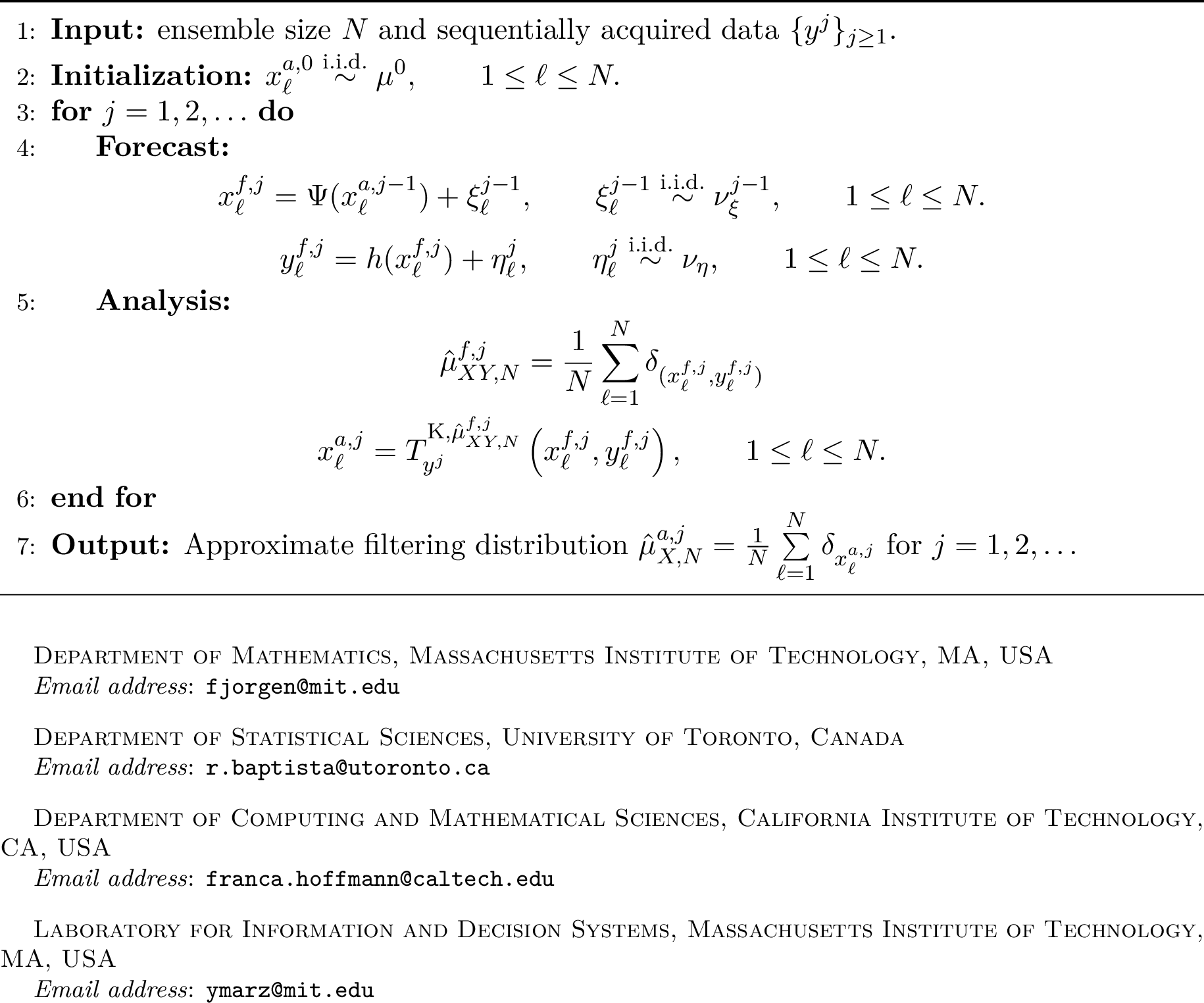
As outlined in Subsection 2.1, the mean-field dynamics associated with Algorithm 3 are given by the distributions \[\label{eq:mf95alg95measure95perspective95enkf} \begin{align} \tilde{\mu}_X^{a,0} &= \mu^0,\\ \tilde{\mu}_X^{a,j} &= \tilde{B}_{y^j}^{\mathrm{K}} Q^j P^{j-1}\tilde{\mu}_X^{a,j-1}, \end{align}\tag{40}\] where \(\tilde{B} ^ {\mathrm{K}}_y\) is the approximate conditioning operator as defined in Equation 19 . To establish the convergence of \(\hat{\mu}_{X,N}^{a,j}\) to \(\tilde{\mu}_{X}^{a,j}\) rigorously, we invoke the general results of Section 3. In order to apply these theorems in the EnKF setting, it remains to verify that the transport map \(T_y^{\mathrm K,\pi}\) in Equation 39 satisfies the required Lipschitz and stability properties in Assumption 2.
Lemma 3. Assume Equation 38 holds. The map \(T^{\mathrm{K},\mu}_{y}\) as defined in Equation 39 for all \(\mu \in \mathcal{P}_2(\mathbb{R}^n \times \mathbb{R}^m)\) and \(y \in \mathbb{R}^m\) satisfies Assumption 2 with the constants in Table ¿tbl:tab:enkf95constants95values?.
Proof. We will show the three conditions required by Assumption 2.
(1a) By definition of \(T^{\text{K},\mu}_{y^\star}\), for all \(x,x^\prime \in \mathbb{R}^n\) and \(y,y^\prime \in \mathbb{R}^m\) it holds that \[\begin{align} &\left\| T^{\text{K},\mu}_{y^\star}(x,y) - T^{\text{K},\mu}_{y^\star}(x^\prime, y^\prime)\right\|_2\\ &\quad = \left\|(x - x^\prime) + \mathrm{Cov}\left(\mu\right)_{XY} \left(\mathrm{Cov}\left(h_\sharp\mu_X\right) + \Lambda\right)^{-1}(y^\prime - y)\right\|_2 \\ &\leq \left( 1 + \left\|\Lambda^{-1}\right\|_{2}\left\|\mathrm{Cov}\left(\mu\right)_{XY}\right\|_{2}\right)\left\|(x,y) - (x^\prime,y^\prime)\right\|_2 \\ &\leq \left( 1 + \left\|\Lambda^{-1}\right\|_{2}{\text{Tr}\mathrm{Cov}\left(\mu\right)}\right)\left\|(x,y) - (x^\prime,y^\prime)\right\|_2 \\ &\leq \left( 1 + \lambda_{\min}^{-1}\right)\left( 1 + {\text{Tr}\mathrm{Cov}\left(\mu\right)}\right)\left\|(x,y) - (x^\prime,y^\prime)\right\|_2, \end{align}\] where we use Equation 38 .
(1b) We abbreviate \(\Delta y = y^\star - y\) and set \[H_\rho\mathrel{\vcenter{:}}= \mathrm{Cov}\left(h_\sharp\rho_X\right), \qquad A_\rho\mathrel{\vcenter{:}}= H_\rho+\Lambda .\] Let \(x \in \mathbb{R}^n\), \(y, y^\star \in \mathbb{R}^m\), \(\nu, \mu \in \mathcal{P}_{2}(\mathbb{R}^n\times\mathbb{R}^m)\). Then, \[\begin{align} \left\| T^{\text{K},\nu}_{y^\star}(x,y) - T^{\text{K},\mu}_{y^\star}(x,y)\right\|_2 &= \left\|\mathrm{Cov}\left(\nu\right)_{XY}A_\nu^{-1}\Delta y - \mathrm{Cov}\left(\mu\right)_{XY}A_\mu^{-1}\Delta y \right\|_2 \\ &\leq \left\|\mathrm{Cov}\left(\nu\right)_{XY}A_\nu^{-1} - \mathrm{Cov}\left(\mu\right)_{XY}A_\mu^{-1}\right\| \left\|\Delta y \right\|_2 \\ &\leq \left\|\Lambda^{-1}\right\|_{2}\left\|\mathrm{Cov}\left(\nu\right)_{XY} - \mathrm{Cov}\left(\mu\right)_{XY}\right\|_{2}\left\|\Delta y \right\|_2 \\ & + \left\|\mathrm{Cov}(\nu)_{XY}\right\|_{2} \left\|A_\nu^{-1}-A_\mu^{-1}\right\|_{2} \left\|\Delta y \right\|_2 \\ &\leq \left\|\Lambda^{-1}\right\|_{2}\left\|\mathrm{Cov}\left(\nu\right) - \mathrm{Cov}\left(\mu\right)\right\|_{2}\left\|\Delta y \right\|_2 \\ & + \left\|\mathrm{Cov}(\nu)\right\|_{2} \left\|A_\nu^{-1}-A_\mu^{-1}\right\|_{2} \left\|\Delta y \right\|_2\\ &\leq \left\|\Lambda^{-1}\right\|_{2}\left\|\mathrm{Cov}\left(\nu\right) - \mathrm{Cov}\left(\mu\right)\right\|_{2} \left\|\Delta y \right\|_2 \\ & + \text{Tr}\mathrm{Cov}(\nu)\left\|\Lambda^{-1}\right\|_{2}^2 \left\| H_\nu - H_\mu\right\|_{2} \left\|\Delta y \right\|_2. \end{align}\] Stacking the covariance matrices together, i.e., inserting \(g(x,y) = ((x,y), h(x))\), verifies (1b).
(3) Finally, let \(\nu \in \mathcal{P}_2\left(\mathbb{R}^n\times\mathbb{R}^m\right), x\in\mathbb{R}^n,y\in\mathbb{R}^m, y^\star \in\mathbb{R}^m\). Then, \[\begin{align} \left\|T^{\text{K},\nu}_{y^\star}(x,y) - x \right\|_2 &= \left\| \mathrm{Cov}(\nu)_{XY}A_\nu^{-1}(y^\star - y)\right\|_2 \\ &\leq \lambda_{\min}^{-1}\left(1 + \text{Tr}\mathrm{Cov}(\nu)\right)\left\|y^\star - y\right\|_2. \end{align}\] ◻
Now, we apply the results of Section 3 to obtain the mean-field convergence of the EnKF as an immediate consequence of Theorem 1 and Lemma 3.
Theorem 2. Fix \(J\in\mathbb{N}_{\ge1}\), draw observations \(Y^{1:J}\) as in Equation 1 (i.e., \(Y^{1:J} \sim \rho^J\) as defined in Equation 26 ) and suppose Assumption 1 holds with time-independent observation noise \(\nu_\eta^j\equiv\nu_\eta\). Assume also that Equation 38 holds. Let \(\{\hat{\mu}_{X,N}^{a,j}\}_{j=1}^{J}\) be the analysis empirical measures for the interacting-particle system produced by Algorithm 3, and let \(\tilde{\mu}^{a,j}_X\) be the mean-field sequence of distributions defined by Equation 40 , both from observations \(y^{1:J}=Y^{1:J}\). Then, for all \(k\ge 2\) and \(N\geq (\log k)^2\), there exists a coupling of i.i.d.particles \(v_\ell^{a,j}\sim\tilde{\mu}_X^{a,j}\) with the interacting ensemble such that the corresponding empirical measure \(\tilde{\mu}^{a,j}_{X,N}=\frac{1}{N}\sum_{\ell=1}^N\delta_{v_\ell^{a,j}}\) satisfies \[\label{eq:EnKF95W295convergence95meanfield} W_2\bigl(\hat{\mu}_{X,N}^{a,j},\tilde{\mu}_{X,N}^{a,j}\bigr) \;\le\;C\frac{(\log k)^{1 +j/2}}{\sqrt{N}} \text{ for all }1 \leq j \leq J,\tag{41}\] with probability at least \(1 - \frac{1}{k}\) over the joint randomness of the particle draws in Algorithm 3 and the observation path \(Y^{1:J}\), where \(C \mathrel{\vcenter{:}}= C(\mathcal{Q})\) depends only on \[\mathcal{Q} \mathrel{\vcenter{:}}= (n,m,\sigma_{\max},\lambda_{\max},\lambda_{\min},\sigma_X,L_\Psi,L_h,J).\] Taking expectations over this randomness yields the non-asymptotic bound \[\mathbb{E}\left(\sup\limits_{1\le j\le J} W_2\bigl(\hat{\mu}_{X,N}^{a,j},\tilde{\mu}_{X,N}^{a,j}\bigr)\right) \le \frac{C'(\mathcal{Q})}{\sqrt{N}},\] for a constant \(C'(\mathcal{Q})\) depending only on \(\mathcal{Q}\).
Theorem 2 establishes the first non-asymptotic, high-probability convergence guarantee in Wasserstein distance for the discrete-time EnKF under general Lipschitz dynamics and observation maps with sub-Gaussian process and observation noise and random observations. The result shows that the empirical EnKF ensemble behaves approximately as i.i.d.samples from its mean-field limit, with the optimal Monte Carlo rate \(N^{-1/2}\) in \(W_2\). Combined with standard i.i.d.concentration inequalities, this yields the dimension-dependent \(W_p\) convergence rate \(N^{-1/n}\) in the high-dimensional regime \(n>2p\). For completeness, we also quantify the \(W_p\)-distance to the mean-field distribution \(\tilde{\mu}_{X}^{a,j}\), which follows directly from Corollary 2.
Corollary 3. Pick any \(p\in[1,2]\). Suppose the conditions in Theorem 2 apply. Then, there exists a constant \(C\geq0\) depending only on \(\mathcal{Q}\) and \(p\) such that for all \(k\ge 2\) and \(N\ge(\log k)^2\), with probability at least \(1-\frac{1}{k}\), we have \[W_p\bigl(\hat{\mu}_{X,N}^{a,j},\tilde{\mu}_X^{a,j}\bigr) \;\le C\left( \gamma_{k,N}^{p,n} +\frac{(\log k)^{1 +j/2}}{\sqrt{N}}\right) \text{ for all }1 \leq j \leq J,\] with the rate \(\gamma_{k,N}^{p,n}\) as in Equation 16 and \[\mathbb{E}\left(\sup\limits_{1\le j\le J} W_p\bigl(\hat{\mu}_{X,N}^{a,j},\tilde{\mu}_X^{a,j}\bigr)\right) \le C \bar\gamma_N^{p,n}.\]
We emphasize that Theorem 2 is, however, the more informative statement: it shows that the EnKF ensemble is (with high probability) as close as possible to an i.i.d.sample from \(\tilde{\mu}_{X}^{a,j}\) at the Monte Carlo scale. Once this i.i.d.behavior is in place, the residual discrepancy to the mean-field is precisely the standard empirical-process error \(\bar\gamma_N^{p,n}\), which reduces to \(N^{-1/n}\) when \(n>2p\) and is known to be sharp in the absence of further assumptions [35].
4.2 Mean-Field Convergence of the EnSMF↩︎
In this subsection, we illustrate how our theory also applies to nonlinear transport ensemble filters by analyzing the ensemble stochastic map filter (EnSMF) [8] as a representative example. The EnSMF generalizes the linear ansatz of the EnKF by learning a (possibly) nonlinear map \(T\) using a variational approach based on samples from the joint forecast distribution. This approach overcomes a limitation of the EnKF’s linear update, which fails to accurately characterize analysis distributions whose dependence on the observations is nonlinear [46], as is the case for general non-Gaussian distributions. We also refer to [8], [47] for evidence of the EnSMF’s lower bias as compared to the EnKF for capturing posterior moments when using nonlinear, rather than linear, transport maps. We introduce stochastic maps and the EnSMF precisely in Subsection 4.2.1 and establish our mean-field convergence result for the EnSMF in Subsection 4.2.2.
4.2.1 Introduction to Stochastic Maps and the EnSMF↩︎
The EnSMF differs from the EnKF (Algorithm 3) only in the analysis step where it replaces the EnKF’s affine map \(T^{\mathrm K}_{y}\) with a (possibly nonlinear) transport map that approximates the exact conditioning operator \(B_{y^\star}\) in Equation 7 for an arbitrary observation \(y^\star\). We begin with an informal sketch of the EnSMF analysis step, whose precise, rigorous formulation will follow.
To define the nonlinear transport, one first seeks a map \(\tilde{S}\colon\mathbb{R}^n\times\mathbb{R}^m\longrightarrow\mathbb{R}^n\times\mathbb{R}^m\) that pushes the joint forecast \(\mu^{f,j}_{XY}\) onto the product distribution of a simple reference measure \(\gamma_\text{G} \in \mathcal{P}_2\left(\mathbb{R}^n \right)\), such as a standard Gaussian, and the marginal measure for the observations \(\mu_Y^{f,j} \in \mathcal{P}_2\left(\mathbb{R}^m \right)\). That is, \[\label{eq:push95forward95condition} \tilde{S}_\sharp\mu_{XY}^{f,j} = \gamma_{\mathrm G}\otimes\mu_Y^{f,j}.\tag{42}\] A convenient structure for conditional simulation is to use invertible transport maps with the block-triangular form \(\tilde{S}(x,y) :=\bigl(S(x,y),y\bigr),\) where both components depend on the observation vector \(y\), but only the first component \(S:\mathbb{R}^n\times\mathbb{R}^m\longrightarrow\mathbb{R}^n\) depends on \(x\). As shown in [48], if the map satisfies Equation 42 , then the inverse of \(x \mapsto S(x,y^j)\), denoted by \(S(\cdot,y^j)^{-1}\), enables posterior sampling via the pushforward \[\mu_{X}^{a,j} = \bigl(S(\cdot,y^j)^{-1}\bigr)_\sharp \gamma_{\mathrm G}.\] This is the main idea behind conditional sampling with triangular transport [49], [50]. In the ensemble-filtering setting, where one uses a particle ensemble to approximate \(\mu_{XY}^{f,j}\), [8] proposes a “prior-to-posterior” scheme that replaces the reference measure \(\gamma_{\mathrm G}\) with samples from the pushforward distribution \(S_\sharp\mu_{XY}^{f,j}\). This yields the conditioning operator \[\label{eq:sm95idea95map} \mu_{X}^{a,j} = \bigl(S(\cdot,y^j)^{-1}\circ S\bigr)_\sharp \mu_{XY}^{f,j}.\tag{43}\] This procedure is called the “stochastic map” and is precisely the analysis step in the EnSMF. It preserves the ensemble size when \(\mu_{XY}^{f,j}\) is replaced by an empirical measure, and it is exact in the case \(\tilde{S}_\sharp\mu_{XY}^{f,j}= \gamma_{\mathrm G}\otimes\mu_Y^{f,j}\). In the following paragraphs we outline the parametric form of the transport map, the learning problem for the map, and regularization techniques for estimating the map.
Map Parameterization. In practice, it is common to construct the map \(S\colon \mathbb{R}^n \times\mathbb{R}^m \rightarrow \mathbb{R}^n\) by considering a parametric family of transport maps \(\mathcal{S}\). Following [8], we define \(S\) to be a strictly triangular map of the form \[S(x,y) = \begin{bmatrix*}[l] S_1(x_1,y) \\ S_2(x_1,x_2,y) \\ \vdots \\ S_n(x_1,\dots,x_n,y) \end{bmatrix*},\] where each component \(S_k\) for \(k=1,\dots,n\) is given by \[\label{eq:S95components} S_k(x,y) = \alpha_k x_k + c_k + \sum_{i=1}^{\iota_k} \theta_k^i f_k^i(x_{1:k-1},y),\tag{44}\] where \(\iota_k \in \mathbb{N}\) and \(\{f_k^i\}_{k=1,\ldots,n; \, i=1,\ldots,\iota_k}\) is a given collection of functions \(f_k^i: \mathbb{R}^{k-1} \times \mathbb{R}^m \to \mathbb{R}\), with the convention that \(x_{1:0}\) is the unique element of \(\mathbb{R}^0\). The parameters of all components are then defined by the coefficients \(\alpha \in \mathbb{R}_{\geq \alpha_{\min}}^n\) for some fixed \(\alpha_{\text{min}} > 0\), \(c \in \mathbb{R}^n\) and scalars \(\{\theta_k^i\}_{k=1,\ldots,n; \, i=1,\ldots,\iota_k}\) with \(\theta_k^i \in \mathbb{R}\). In what follows, we rewrite the coefficients \(\{\theta_k^i\}_{k,i}\) and functions \(\{f_k^i\}_{k,i}\) using vectors: \[\begin{align} \theta_k &\mathrel{\vcenter{:}}= \left( \theta_k^1, \ldots, \theta_k^{\iota_k}\right)^\top \\ f_k &\mathrel{\vcenter{:}}= \left( f_k^1, \ldots, f_k^{\iota_k}\right)^\top. \end{align}\] When a full state vector is supplied as the first argument, \(f_k^i(x,y)\) means \(f_k^i(x_{1:k-1},y)\), and \(f_k(x,y)\) means the corresponding vector of feature evaluations. We write \(\iota\mathrel{\vcenter{:}}=(\iota_1,\ldots,\iota_n)\) for the vector of feature dimensions. Moreover, we will write \(S = \mathcal{S}(\alpha, c, \theta) \in \mathcal{S}\) to denote instances of such maps in the parametric family \(\mathcal{S}\). For our results, the functions \(f_k^i\) are assumed to satisfy the following conditions.
Assumption 3. For each \(k \in \{1, \ldots, n\}\), we have
Lipschitz continuity: Each function \(f_k\) is \(L_f\)-Lipschitz for a fixed constant \(L_f \geq 0\).
Differentiability: Each function \(f_k^i\) is continuously differentiable in \(x\).
Triangular variable dependence: For each \(i \in \{1,\ldots, \iota_k\}\) and \(j \geq k\), \(\partial_{x_j}f_k^i =0\).
Concrete choices of the basis functions \(f_{k}^i\), as described in [8], include polynomial (monomial) bases—typically regularized at infinity to ensure global Lipschitz continuity—and Gaussian radial basis functions. Both of these examples satisfy Assumption 3.
Learning the Map. As explained at the beginning of this section, a natural approach is to choose \(S\) so that \(\tilde{S}_\sharp\mu\) has small Kullback–Leibler (KL) divergence from \(\gamma_{\mathrm G}\otimes\mu_Y\). When this quantity is well defined, this approach leads to the variational problem \[\label{eq:KL95min95sm} \min_{S \in \mathcal{S}} D_{\mathrm{KL}}\bigl(\tilde{S}_\sharp\mu\,\|\,\gamma_{\mathrm G}\otimes\mu_Y\bigr),\tag{45}\] with \(\tilde{S}(x,y)\mathrel{\vcenter{:}}=(S(x,y),y)\), where \(D_{\mathrm{KL}}(\pi\,\|\,\pi')\) denotes the KL divergence from \(\pi\) to \(\pi'\). As is typical in stochastic-map constructions [8], [49], we take \(\gamma_{\mathrm G}=\mathcal{N}(0,I_n)\) as the reference measure. The triangular structure of \(S\), together with the constraint \(\alpha_k\ge \alpha_{\min}>0\), implies—by a straightforward induction over the state dimension—that, for every \(S\in\mathcal{S}\) and \(y\in\mathbb{R}^m\), the map \(S(\cdot,y):x\mapsto S(x,y)\) is a diffeomorphism; see Lemma 6 in the Appendix. Thus the pullback measure \(\left(S(\cdot, y)\right)^\sharp\gamma_{\mathrm G}\mathrel{\vcenter{:}}= \left(S(\cdot, y)^{-1}\right)_\sharp\gamma_{\mathrm G}\) has a density.
To avoid potential well-posedness issues in Equation 45 , while preserving its minimizers whenever the KL formulation is valid, we choose \(S\) directly as the maximum-likelihood estimator, i.e., as a minimizer of the cross-entropy objective [8], [49] \[\label{eq:cross95entropy95min95sm} \min_{S \in \mathcal{S}} -\int \mathrm{d}\mu(x,y)\log \left(\left(S(\cdot, y)\right)^\sharp\gamma_{\mathrm G}\right)(x).\tag{46}\] This objective depends on the joint distribution \(\mu\) only through the expectation and is therefore amenable to empirical approximation, e.g., using forecast samples. The following result shows that, under suitable conditions, the Gaussian reference choice \(\gamma_{\mathrm G}\) leads to a well-posed stochastic-map optimization in Equation 46 . A proof is included in the Appendix.
propositionpropexistenceminimizer Let \(\mu \in\mathcal{P}_2\left(\mathbb{R}^n \times \mathbb{R}^m \right)\) satisfy \(\mathrm{Cov}\left(\left( f_k\right)_\sharp \mu \right) \succ 0\) and \[R_k(\mu) \mathrel{\vcenter{:}}= \mathrm{Cov}\left(X_k\right) - \mathrm{Cov}\left( f_k(X,Y), X_k \right) ^\top\mathrm{Cov}\left( f_k(X,Y) \right)^{-1} \mathrm{Cov}\left( f_k(X,Y), X_k \right) > 0,\] for every \(k = 1, \ldots, n\) and \((X, Y) \sim \mu\). Then, Equation 46 has a unique minimizer \(S^\mu \in \mathcal{S}\) that is defined by the parameters \[\label{eq:params95sm} \begin{align} \alpha_k &= \max\left(\frac{1}{\sqrt{R_k(\mu)}}, \alpha_{\min}\right) \\ \theta_k &= - \alpha_k \mathrm{Cov}\left( f_k(X,Y) \right)^{-1} \mathrm{Cov}\left( f_k(X,Y), X_k \right) \\ c_k &=- \mathbb{E}\left(\alpha_kX_k + \sum_{i=1}^{\iota_k} \theta_k^i f_k^i(X_{1:k-1},Y)\right). \end{align}\tag{47}\]
For suitable \(\mu \in\mathcal{P}_2\left(\mathbb{R}^n\times\mathbb{R}^m\right)\) satisfying the condition in Proposition [prop:existence95minimizer95sm95KL] and \(y^\star \in \mathbb{R}^m\), we now construct the prior-to-posterior transport map in 43 that defines the approximate conditioning operator \(\tilde{B}_{y^\star}\) using the stochastic map \[T_{y^\star}^{\mu}(x,y) := \left(S^\mu(\cdot,y^\star)^{-1}\circ S^\mu\right)(x,y).\] For the map components in Equation 44 , we obtain a closed form for the stochastic map by direct calculation. Defining the map’s output as \(w = T_{y^\star}^\mu(x,y) \in \mathbb{R}^n\), the following recursive equations hold for all \(k\geq 1\) with \(\alpha, \theta\) defined as in Proposition [prop:existence95minimizer95sm95KL]: \[w_k = x_k + \frac{\theta_k^\top}{\alpha_k} \left(f_k(x,y) -f_k(w,y^\star)\right).\] Since \(w_k\) depends only on the ratio \(\frac{\theta_k}{\alpha_k} = -\mathrm{Cov}\!\left(f_k(X,Y)\right)^{-1}\mathrm{Cov}\!\left(f_k(X,Y), X_k\right),\) the definition can be naturally extended to cases where \(R_k(\mu)=0\) by defining the stochastic map directly in terms of the moments of \(\mu\). Defining the map’s output as \(\chi_{y^\star}(x,y;\theta) \in \mathbb{R}^n\) with \(\theta_k \in \mathbb{R}^{\iota_k}\) for each \(k\), the following recursive equations hold: \[\label{eq:sm95approximate95conditioning95recursion} (\chi_{y^\star}(x,y;\theta))_k = x_k - \theta_k^\top\left(f_k(x,y) -f_k(\chi_{y^\star}(x,y),y^\star)\right).\tag{48}\] Indeed, under the assumptions of Proposition [prop:existence95minimizer95sm95KL], the prior-to-posterior map \(T_{y^\star}^{\mu}\) obtained from the minimizer \(S^\mu\) in Equation 46 coincides with \(\chi_{y^\star}(\cdot,\cdot;\theta)\) when \[\theta_k = \mathrm{Cov}\left( f_k(X,Y) \right)^{-1} \mathrm{Cov}\left( f_k(X,Y), X_k \right).\]
Map Regularization. To extend this expression stably when \(\mathrm{Cov}\!\left(f_k(X,Y)\right)\) is singular or ill-conditioned, it is common to incorporate regularization of the covariance matrix [8]. Given a symmetric matrix \(C \in \mathbb{R}^{u \times u}\) and a regularization constant \(\upsilon> 0\), we define \(C_{\upsilon}\) as the closest positive semidefinite approximation to \(C\) that is bounded below by \(\upsilon I_{u}\). That is \[\label{eq:frob95proj} C_{\upsilon} = \mathop{\mathrm{arg\,min}}_{\tilde{C} \succeq \upsilon I_{u}} \left\|\tilde{C} - C\right\|_F^2.\tag{49}\] With a fixed regularization level \(\hat{\sigma}_f>0\), we define the stochastic map for \(y^\star \in \mathbb{R}^m\) and any \(\mu \in \mathcal{P}_2\left(\mathbb{R}^n\times\mathbb{R}^m\right)\) as \[\label{eq:alg95conditioning95transport95SM} T^{\mathrm{SM},\mu}_{y^\star}(x,y) = \chi_{y^\star}(x,y;\theta),\tag{50}\] for the parameter \(\theta_k \mathrel{\vcenter{:}}= \mathrm{Cov}_{\hat{\sigma}_f}\left( f_k( X, Y) \right)^{-1} \mathrm{Cov}\left( f_k( X, Y), X_k \right)\) and \((X, Y) \sim \mu\), where \(\mathrm{Cov}_{\hat{\sigma}_f}(Z)\mathrel{\vcenter{:}}=(\mathrm{Cov}(Z))_{\hat{\sigma}_f}\).
The update step in 50 results in the transport ensemble filter. Taking \(\mu\) to be the empirical measure from the forecast step yields the ensemble stochastic map filter, which is summarized in Algorithm 4.
Remark 11. Alternative regularizations (e.g., Tikhonov) lead to an essentially identical analysis and comparable bounds. Here, we adopt the projection scheme in 49 , which is equivalent to eigenvalue thresholding, because it yields a cleaner and more informative mean-field limit. A brief note on the computational implementation of this scheme is provided in Appendix 5.6.
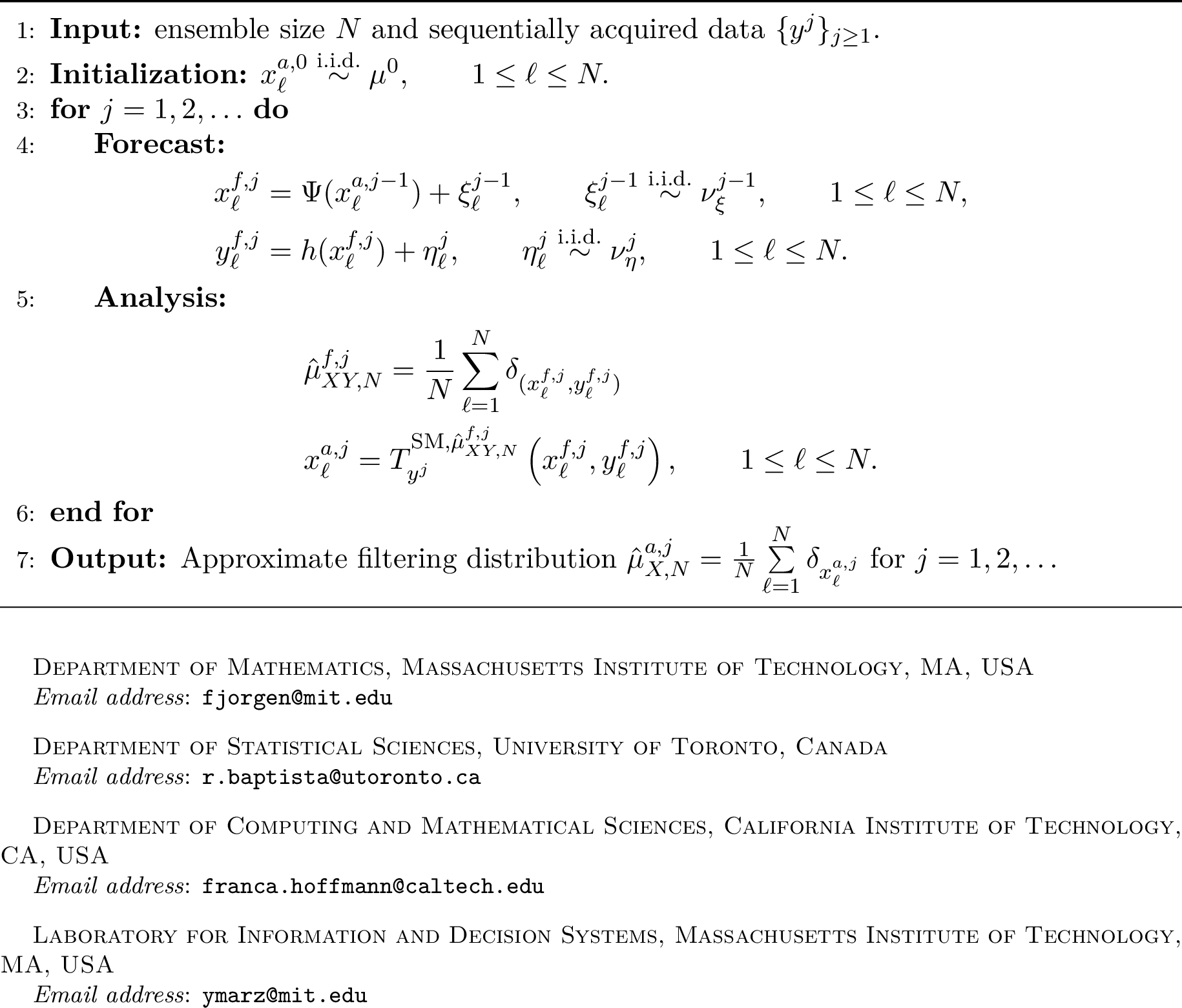
4.2.2 Convergence Result↩︎
As in Subsection 2.1, the mean-field dynamics to which the ensemble \(\hat{\mu}_{X,N}^{a,j}\) produced by Algorithm 4 converges are given by \[\label{eq:ensmf95mf95alg95measure95perspective} \begin{align} \tilde{\mu}_{X}^{a, 0} &= \mu^0 \\ \tilde{\mu}_{XY}^{f, j} &=Q^jP^{j-1}\tilde{\mu}_X^{a,j-1} \\ \tilde{\mu}_{X}^{a,j} & = \tilde{B}^{\text{SM}}_{y^j} \tilde{\mu}_{XY}^{f, j} \end{align}\tag{51}\] where \(\tilde{B}^{\text{SM}}_y\) is defined in Equation 19 . To prove this statement rigorously, we rely on the results from Section 3 and establish that Assumption 2 is satisfied for the map \(T_{y}^{\mathrm{SM},\mu}\) at any analysis step of the algorithm in the following lemma.
lemmalemsmfassumptions \(T^{\mathrm{SM},\mu}_y\) satisfies Assumption 2 with constants depending only on the quantities introduced in Assumptions 1 and 3, on the feature dimensions \(\iota\), and on the regularization level \(\hat{\sigma}_f\).
A proof of this lemma can be found in Appendix 5.7 and we can now invoke the general results of Section 3 to obtain mean-field convergence of the EnSMF as a direct consequence of Theorem 1 together with Lemma [lem:smf95satisfies95assumptions].
Theorem 3. Fix \(J\in\mathbb{N}_{\ge1}\) and draw \(Y^{1:J}\) as in Equation 1 , i.e., \(Y^{1:J} \sim \rho^J\) as defined in Equation 26 . Suppose Assumptions 1 and 3 hold. Let \(\{\hat{\mu}_{X,N}^{a,j}\}_{j=1}^{J}\) be the analysis empirical measures produced by Algorithm 4, and let \(\tilde{\mu}^{a,j}_X\) be the mean-field sequence defined by Equation 51 with observations \(y^{1:J}=Y^{1:J}\). Then there exists a coupling of i.i.d.particles \(v_\ell^{a,j}\sim\tilde{\mu}_X^{a,j}\) with the interacting ensemble such that the corresponding empirical measure \(\tilde{\mu}^{a,j}_{X,N}=\frac{1}{N}\sum_{\ell=1}^N\delta_{v_\ell^{a,j}}\) satisfies, for all \(k\ge 2\) and \(N\geq (\log k)^2\), with probability at least \(1 - \tfrac1k\) \[W_2\bigl(\hat{\mu}_{X,N}^{a,j},\tilde{\mu}_{X,N}^{a,j}\bigr) \;\le\;C\frac{(\log k)^{1 +j/2}}{\sqrt{N}} \text{ for all }1 \leq j \leq J,\] where \(C\mathrel{\vcenter{:}}= C(\mathcal{Q})\) depends only on \[\mathcal{Q} \mathrel{\vcenter{:}}= (n,m,\sigma_{\max},\lambda_{\max},\sigma_X,L_\Psi,L_h,L_f, \hat{\sigma}_f,\iota,J).\] The randomness is over both the particle draws in Algorithm 4 and the observation path \(Y^{1:J}\). Moreover, we have the non-asymptotic bound \[\mathbb{E}\left(\sup\limits_{1\le j\le J} W_2\bigl(\hat{\mu}_{X,N}^{a,j},\tilde{\mu}_{X,N}^{a,j}\bigr)\right) \le \frac{C'(\mathcal{Q})}{\sqrt{N}},\] for a constant \(C'(\mathcal{Q})\) depending only on \(\mathcal{Q}\).
As for the EnKF, we include a result for the convergence of \(\hat{\mu}_{X,N}^{a,j}\) to the mean-field \(\tilde{\mu}_{X}^{a,j}\) in the \(W_p\) distance. The proof of this result follows the same steps as Corollary 2.
Corollary 4. Consider the same setting as in Theorem 3 and choose any \(p\in[1,2]\). Then, there exists a constant \(C \geq 0\) depending only on \(\mathcal{Q}\) and \(p\) such that for all \(k\ge 2\) and \(N\geq (\log k)^2\), with probability at least \(1-\frac{1}{k}\), \[W_p\bigl(\hat{\mu}_{X,N}^{a,j},\tilde{\mu}_X^{a,j}\bigr) \;\le C\left(\gamma_{k,N}^{p,n}+\frac{(\log k)^{1 +j/2}}{\sqrt{N}}\right) \text{ for all }1 \leq j \leq J,\] with the rate \(\gamma_{k,N}^{p,n}\) as in Equation 16 and \[\mathbb{E}\left(\sup\limits_{1\le j\le J}W_p\bigl(\hat{\mu}_{X,N}^{a,j},\tilde{\mu}_X^{a,j}\bigr)\right)\le C \bar\gamma_N^{p,n}.\]
5 Auxiliary Results↩︎
5.1 Auxiliary Results for Section 3.1↩︎
For the empirical-measure concentration result below, define \[\gamma_{k,N}^{p,d} = \begin{cases} \Bigl(\frac{\log k}{N}\Bigr)^{1/d} &\text{if } 1\le p < \frac{d}{2}\\ \Bigl(\frac{\log k}{N}\Bigr)^{1/d}\bigl(\log(2+N)\bigr)^{2/d} &\text{if } p = \frac{d}{2}\\ \Bigl(\frac{\log k}{N}\Bigr)^{1/(2p)} &\text{if } \frac{d}{2} < p \le 2\,, \end{cases}\] and \[\tilde{\gamma}_{k,N}^{p,d} \mathrel{\vcenter{:}}= \max\left\{\gamma_{k,N}^{p,d},\sqrt{\frac{\log k}{N}}\right\}.\] For convenience, we also recall the corresponding \(k\)-free empirical-measure rate \[\bar\gamma_N^{p,d} = \begin{cases} N^{-1/d} &\text{if } 1\le p < \frac{d}{2},\\ N^{-1/d}\bigl(\log(2+N)\bigr)^{2/d} &\text{if } p = \frac{d}{2},\\ N^{-1/(2p)} &\text{if } \frac{d}{2} < p \le 2. \end{cases}\]
Proposition 9. Let \(d\geq1\) and \(p\in[1,2]\). Let \((X_i)_{i=1}^N\) be i.i.d.\(\mathbb{R}^d\)-valued with law \(\mu\), and let \(\mu_N\) be the empirical measure. Assume the centered sub-Gaussian condition \[\big\|X_i-\mathbb{E} X_i\big\|_{2,\psi_2}\le K .\] Then there exists a constant \(A_1\geq 0\), depending only on \(d,p,K\), such that for all \(N\ge1\) and \(k\ge2\) \[\mathbb{P}\left(W_p(\mu_N,\mu)\;\ge A_1 \tilde{\gamma}_{k,N}^{p,d}\right)\;\le\;\frac{1}{k}\,.\] Moreover, there exists a constant \(A_2> 0\), depending only on \(d,p,K\), such that for all \(N\ge1\), \[\mathbb{E}W_p(\mu_N,\mu)\le A_2 \bar\gamma_N^{p,d}\,.\]
Proof. By the sub-Gaussian assumption \[\mathbb{E}\exp\bigl(\| X-\mathbb{E}X\|_2^2/K^2\bigr) \leq 2< \infty.\] Since a translation does not change Wasserstein distances, we may assume \(\mathbb{E}X=0\) and thus \(\int e^{\|y\|_2^2/K^2}\mu(dy) < \infty.\) This is the exponential-moment assumption of Example 3.4 in [34], with \(\beta=2\ge p\) and constants depending only on \(d,p,K\). Let \(\mathcal{T}_p(\mu,\nu):=W_p(\mu,\nu)^p\). Example 3.4(a) with \(\beta=2\) gives, for all \(N\in\mathbb{N}\), \(x>0\), \[\mathbb{P}\bigl(\mathcal{T}_p(\mu,\mu_N)>x\bigr) \le C_1\exp\bigl(-c_1 N\phi(x)\bigr)\mathrm 1_{\{x\le1\}} + C_1\exp\bigl(-c_1 N x^{2/p}\bigr)\mathrm 1_{\{x\ge1\}},\] where the rate function \(\phi\) (depending on \(d,p\)) is \[\phi(x) = \begin{cases} x^2 & p>\frac{d}{2}\\ \bigl(x/\log(2+1/x)\bigr)^2 & p=\frac{d}{2}\\ x^{d/p} & 0<p<\frac{d}{2}. \end{cases}\] Plugging in \(x = t^p\) gives \[\mathbb{P}\bigl(W_p(\mu_N,\mu)>t\bigr) = \mathbb{P}\bigl(\mathcal{T}_p(\mu,\mu_N)>t^p\bigr) \le C_1\exp\bigl(-c_1 N\phi(t^p)\bigr) + C_1\exp\bigl(-c_1 N t^{2}\bigr).\] For \(t =A_1 \tilde{\gamma}_{k,N}^{p,d}\) the second term is upper bounded by \((2k)^{-1}\) for sufficiently large \(A_1 \geq 0\) since \(\tilde{\gamma}_{k,N}^{p,d} \geq \left(\log k/N \right)^{1/2}\) and \(\log(2k)\le 2\log k\) for \(k\ge2\). Similarly, plugging in \(t =A_1 \tilde{\gamma}_{k,N}^{p,d} \geq A_1\gamma_{k,N}^{p,d}\) for the first term and some elementary algebra in each of the three cases shows that it is smaller than \((2k)^{-1}\) for sufficiently large \(A_1 \geq 0\). The two bounds sum to the claimed failure probability \(k^{-1}\).
The expectation bound follows by the layer-cake representation. ◻
5.2 Auxiliary Results for Section 3.2↩︎
We derive the auxiliary results used in Subsection 3.2. We start by giving a routine argument for the stability of \(\|\cdot\|_{2,\psi_2}\) under Lipschitz maps as we will apply this property repeatedly.
Proposition 10. Let \(X\in \mathbb{R}^{u_1}\) be a random vector such that \(\|X - \mathbb{E}(X)\|_2\) is sub-Gaussian. Assume that \(f:\mathbb{R}^{u_1}\rightarrow\mathbb{R}^{u_2}\) is \(L\)-Lipschitz. Then \[\left\|f(X) - \mathbb{E}f(X)\right\|_{2,\psi_2} \leq 2L \left\| X - \mathbb{E}(X)\right\|_{2,\psi_2}.\]
Proof of Proposition 10. Consider \(X^\prime\), an independent copy of \(X\). By repeatedly applying Jensen’s inequality and independence, we find \[\begin{align} \left\|f(X) - \mathbb{E}f(X)\right\|_{2,\psi_2}&= \inf \left\{t>0: \mathbb{E}\left(e^{ \left\|f(X) - \mathbb{E}f(X^\prime)\right\|_2^2 / t^{2}}\right) \leq 2\right\}\\ & \leq \inf \left\{t>0: \mathbb{E}\exp\left(\frac{\|f(X)-f(X^\prime)\|_2^2}{t^2}\right) \leq 2\right\}\\ & \leq \inf \left\{t>0: \mathbb{E}\left(e^{ \left\|X - X^\prime\right\|_2^2 / (t/L)^{2}}\right) \leq 2\right\}\\ & = \inf \left\{t>0: \mathbb{E}\left(e^{ \left\|(X- \mathbb{E}(X)) - (X^\prime - \mathbb{E}(X))\right\|_2^2 / (t/L)^{2}}\right) \leq 2\right\}\\ & \leq \inf \left\{t>0: \mathbb{E}\left(e^{ 2\left(\left\|X- \mathbb{E}(X)\right\|_2^2+ \left\|X^\prime - \mathbb{E}(X)\right\|_2^2\right) / (t/L)^{2}}\right) \leq 2\right\}\\ & = \inf \left\{t>0: \mathbb{E}\left(e^{ 2\left(\left\|(X- \mathbb{E}(X))\right\|_2^2\right) / (t/L)^{2}}\right)^2 \leq 2\right\}\\ & \leq \inf \left\{t>0: \mathbb{E}\left(e^{ 4\left\|X- \mathbb{E}(X)\right\|_2^2 / (t/L)^{2}}\right)\leq 2\right\}\\ &= \inf \left\{t>0: \mathbb{E}\left(e^{ \left\|X- \mathbb{E}(X)\right\|_2^2 / (t/2L)^{2}}\right)\leq 2\right\}\\ &= 2L \inf \left\{t>0: \mathbb{E}\left(e^{ \left\|X- \mathbb{E}(X)\right\|_2^2 / t^{2}}\right)\leq 2\right\}\\ &= 2L \left\|X - \mathbb{E}X\right\|_{2,\psi_2}. \end{align}\] ◻
Now, we can prove Lemma 1.
Proof of Lemma 1. We prove by induction that \(\|X^j-\mathbb{E}(X^j)\|_2\) is sub-Gaussian.
For the base case, \(\left\|X^0\right\|_{2,\psi_2} \leq \sigma_X < \infty\) by Assumption 1. By \(\|X^0 - \mathbb{E}(X^0)\|_2 \leq \|X^0\|_2 + \mathbb{E}(\|X^0\|_2)\) we have \(\|X^0 - \mathbb{E}(X^0)\|_{2,\psi_2}\leq 2\sigma_X\) (see also Exercise 2.40e of [43] for tighter centering bounds). Let \(j\geq 0\) and \(\|X^{j} - \mathbb{E}(X^{j})\|_2\) be sub-Gaussian with norm bounded by a constant depending on the parameters in the statement. We have \(X^{j+1} = \Psi(X^j) + \xi^j\) and \(\|\Psi(X^j) - \mathbb{E}(\Psi(X^j))\|_2\) is sub-Gaussian by Proposition 10. Further, \[\|\Psi(X^j) + \xi^j - \mathbb{E}(\Psi(X^j) + \xi^j)\|_2 \leq \|\Psi(X^j) - \mathbb{E}(\Psi(X^j))\|_2 + \|\xi^j - \mathbb{E}(\xi^j)\|_2\] and by triangle inequality of the Orlicz norm the right-hand-side is sub-Gaussian. By sub-Gaussian summation properties, this also shows that the left-hand side \(\left\|X^{j+1} - \mathbb{E}(X^{j+1})\right\|_2\) is sub-Gaussian. This shows that all \(X^j, 1\leq j \leq J\) are sub-Gaussian with sub-Gaussian norm upper bounded by a parameter depending only on \(\sigma_X, \sigma_{\max}, L_\Psi, J\). \(\|Y^j - \mathbb{E}(Y^j)\|_2\) is sub-Gaussian by the same argument since \(Y^j = h(X^j) + \eta^j,\) \(h\) is Lipschitz, and \(\eta^j\) is sub-Gaussian. The final result follows with \[\left\|(X^j, Y^j) - \mathbb{E}(X^j, Y^j)\right\|_2 \leq \left\|X^j- \mathbb{E}(X^j)\right\|_2+ \left\|Y^j- \mathbb{E}(Y^j)\right\|_2.\] We emphasize that each of the cited results demonstrates the stability of sub-Gaussian behavior under operations such as addition, upper bounding, and Lipschitz transformations, with constants that depend solely on the parameters characterizing the sub-Gaussian and Lipschitz parameters. ◻
Further, we used Proposition 2 in the proof of Proposition 1 and here, we give a short proof.
Proof of Proposition 2. By Jensen’s inequality, \[\begin{align} e^{\left\|\mathbb{E}(X|Y) / t\right\|_2^{2}} \le \mathbb{E}\left(e^{\|X / t\|_2^{2}}\,|\,Y\right) \end{align}\] conditional on \(Y\), and hence \[\begin{align} \left\|\mathbb{E}(X|Y)\right\|_{2,\psi_2} &= \inf \left\{t>0: \mathbb{E}\left(e^{\left\|\mathbb{E}(X|Y) / t\right\|_2^{2}}\right) \leq 2\right\} \\ &\leq \inf \left\{t>0: \mathbb{E}\left(e^{\|X / t\|_2^{2}}\right) \leq 2\right\} \\ &= \|X\|_{2,\psi_2} . \end{align}\] ◻
To prove Proposition 5, we rely on the following lemma.
Lemma 4. Let \(c >0\). Then, \[\sum\limits_{n = 0}^\infty \exp(-c2^{2n}) \leq \exp({-c})\left(1+\frac{1}{c\log 4}\right).\]
Proof. For \(c>0\), let \(f(x)=\exp({-c4^x})\). Since \(f\) is positive and decreasing on \([0,\infty)\), \[\sum_{j=0}^\infty f(j) \le f(0)+\int_0^\infty f(x)\,dx = \exp({-c})+\int_0^\infty \exp(-c4^x)\,dx.\] With \(t=4^x\) so \(dx=\frac{dt}{t\log 4}\), \[\int_0^\infty \exp(-c4^x)dx = \int_{1}^{\infty}\frac{\exp(-ct)}{t\log 4}dt = \frac{1}{\log 4}\int_{c}^{\infty}\frac{\exp(-u)}{u}du \le \frac{\exp(-c)}{c\log 4}.\] Hence \[\sum_{j=0}^\infty \exp(-c4^j) \le \exp({-c})\left(1+\frac{1}{c\log 4}\right).\] ◻
Now, we prove our new characterization of sub-Gaussianity.
Proof of Proposition 4. Assume there exists a constant \(K_5\) such that for any \(|t|\geq 1/K_5\) it holds that \(\mathbb{E}(\exp(tX)) \leq \exp\left( t^2K_5^2\right).\) Fix \(x\geq 2K_5\). For any \(|\lambda| \geq1/K_5\), a Chernoff bound gives \[\mathbb{P}\bigl(X \geq x\bigr) \le \exp(-\lambda x) \mathbb{E}\left(\exp(\lambda X)\right) {\le} \exp\!\Bigl( -\lambda x + \lambda^{2}K_5^{2} \Bigr).\] Minimizing the exponent in \(\lambda\) gives \(\lambda^{\star}=x/(2K_5^{2})\), which is valid for the Chernoff bound since \(|\lambda^{\star}|=|x|/(2K_5^{2}) = x/(2K_5^{2}) \geq1/K_5\). Hence, \(\mathbb{P}\bigl(X \geq x\bigr) \le \exp\left(-\frac{x^{2}}{4K_5^{2}}\right).\) It follows by applying the same argument to \(-X\) and a union bound that for all \(x \geq 2K_5\), \(\mathbb{P}\bigl(|X | \geq x\bigr) \le 2\exp\!\left(-\frac{x^{2}}{4K_5^{2}}\right).\) For \(K_2 = \frac{2K_5}{\sqrt{\log 2}}\), we have that \[\mathbb{P}\bigl(|X | \geq x\bigr) \le 2\exp\!\left(-\frac{x^{2}}{K_2^2}\right)\] for all \(x\geq 0\): For \(x \geq 2K_5\) this follows from what we just showed, i.e., \(\mathbb{P}\bigl(|X | \geq x\bigr) \le 2\exp\left(-\frac{x^{2}}{4K_5^2}\right) \leq 2\exp\left(-\log 2\frac{x^{2}}{4K_5^2}\right) = 2\exp\left(-\frac{x^{2}}{K_2^2}\right)\), as \(\log 2 < 1\). For \(0 \leq x\leq 2K_5\), we have \(2\exp\left(-\frac{x^{2}}{K_2^2}\right) \geq 2\exp\left(-\log 2\frac{4K_5^2}{4K_5^2}\right) = 1\), so it is trivially true. This shows sub-Gaussianity by Proposition 3 with \(K_2 = \frac{2}{\sqrt{\log 2}}K_5\). Conversely, let \(X\) be sub-Gaussian and write \(K_1=\|X\|_{\psi_2}\). By Proposition 3, the tail bound in Property 2 holds for some \(K_2\le \tilde{C}_{\psi_2}K_1\). Then, the moment generating function exists for any \(t \in \mathbb{R}\). The case \(t=0\) is immediate, so let \(t > 0\) and apply the layer-cake representation as well as Property 2 in Proposition 3: \[\begin{align} \mathbb{E}\exp(tX) & = \int\limits_0^\infty \mathbb{P}\left(\exp(tX)\geq s\right)\mathrm{d}s \\ &\leq 1 + \int\limits_1^\infty \mathbb{P}\left(\exp(tX)\geq s\right)\mathrm{d}s\;=\; 1 + \int\limits_1^\infty \mathbb{P}\left(X\geq \frac{\log s }{t}\right)\mathrm{d}s \\ &= 1 + t\int\limits_0^\infty \exp(tu)\mathbb{P}\left(X\geq u\right)\mathrm{d}u \;\leq\; 1 + 2t\int\limits_{0}^\infty \exp(tu)\exp\left(-\frac{u^2}{K_2^2}\right)\mathrm{d}u\\ &\leq 1 + 2t\int\limits_{-\infty}^\infty \exp(tu)\exp\left(-\frac{u^2}{K_2^2}\right)\mathrm{d}u \;=\; 1 + 2\sqrt{\pi t^2K_{2}^2} \cdot \exp \left(\frac{t^{2} K_{2}^2}{4}\right) \\ \end{align}\] Now, note that the function \(\alpha x\exp(-\beta x^2)\) restricted to \(x\geq 0\) has its maximum value at \(\frac{\alpha}{\sqrt{2\beta}}\exp(-1/2)\). Choosing \(\alpha = 2 \sqrt{\pi}\) and \(\beta = 2\pi\) yields \(2 \sqrt{\pi} x \exp(-2\pi x^2) \leq 1\) for all \(x \geq 0\). Therefore, we can further bound, for \(x = K_2 t\), \[\begin{align} \mathbb{E}\exp(tX) &\leq 1 + 2\sqrt{\pi} x \exp\left(- 2\pi x^2\right) \cdot \exp \left( \frac{x^2}{4} + 2\pi x^2\right) \\ & \leq 1 + 1 \cdot \exp \left(\left(\frac{1}{4} + 2\pi\right){t^{2} K_{2}^2}\right) \\ &\leq \exp \left(\underbrace{\left(\frac{1}{4} + 2\pi\right)K_2^2}_{=:\tilde{K}_2^2}\cdot {t^{2}} + \log 2\right). \end{align}\] We can generalize this to all \(t\in \mathbb{R}\) by applying the same argument to \(-X\) which is sub-Gaussian with the same parameter to obtain \[\mathbb{E}\exp(tX)\leq \exp \left(\tilde{K}_2^2 {t^{2}} + \log 2\right) \forall t\in\mathbb{R}.\] Now, choose \(K_5 = 4 \tilde{K}_2\). Let \(|t|\geq \frac{1}{K_5}\). We have \[\begin{align} t^2 K_5^2 - \left({t^{2} \tilde{K}_{2}^2}+ \log2\right)& = t^2\tilde{K}_2^2\left( 16- 1\right)- \log2 \;\geq\; \frac{15}{16} - \log2 \;\geq\; 0. \end{align}\] In particular, \[\mathbb{E}\exp(tX) \leq \exp(K_5^2t^2), \quad \forall |t| \geq \frac{1}{K_5}\] and we are done with the reverse bound since \(K_5 = 4\sqrt{1/4+2\pi}K_2\). Thus, with \[C_{\psi_2}\mathrel{\vcenter{:}}= \max\left(1,\tilde{C}_{\psi_2},\frac{2\tilde{C}_{\psi_2}}{\sqrt{\log 2}},4\sqrt{1/4+2\pi}\tilde{C}_{\psi_2}\right)\,,\] the first direction gives \(\|X\|_{\psi_2}\le C_{\psi_2}K_5\) whenever 27 holds with parameter \(K_5\), while the reverse direction gives an admissible \(K_5\le C_{\psi_2}\|X\|_{\psi_2}\). We conclude by showing the monotonicity property. Assume Equation 27 holds and let \(\tilde{K}_5 > K_5\). For \(|t| \geq 1/K_5\) there is nothing to show, so let \(1/\tilde{K}_5 \leq |t| \leq 1/K_5\). Without loss of generality, \(t\geq 0\) since we can apply the same argument to \(-X\). Decompose convexly as \(t = (1-p) \cdot 0 + p\cdot 1/K_5\), so \(p=K_5t\). By log-convexity of the moment generating function, we have that \[\log \mathbb{E}(\exp(tX)) \leq p \log \mathbb{E}(\exp(X/K_5)) \leq p \log e = p.\] We are done since \(p=K_5t\le \tilde{K}_5t\le \tilde{K}_5^2t^2\), where the last inequality uses \(t\ge 1/\tilde{K}_5\). ◻
Remark 12. Alternatively, the reverse direction follows directly from the Orlicz characterization: if \(\mathbb{E}\exp(X^{2}/K_{1}^{2})\le 2\), then the inequality \(ab\le \tfrac{a^{2}}{2}+\tfrac{b^{2}}{2}\) (applied to \(a=\sqrt{2}X/K_{1}\) and \(b=tK_{1}/\sqrt{2}\)) gives \[e^{tX}\le \exp\left(\frac{X^{2}}{K_{1}^{2}}\right)\exp\left(\frac{K_{1}^{2}t^{2}}{4}\right),\] and taking expectations immediately yields the desired mgf bound for large \(|t|\) - the proof can be completed for small \(|t|\) after some additional algebra.
5.3 Auxiliary Result for Subsection 3.3↩︎
We present a proof of Proposition 6.
Proof of Proposition 6. Fix the observation path \(y^{1:J}\) throughout this proof. Construct the mean-field dynamics \(\tilde{Z}^j_f\mathrel{\vcenter{:}}= (\tilde{X}^j_f, \tilde{Y}^j_f) \sim \tilde{\mu}^{f,j}_{XY}\) at different times on a common probability space by drawing independently \(X^0\sim \mu^0\), \(\{\xi^{t}\}_{t \ge 0}\) with \(\xi^{t} \sim \nu_\xi^t\), \(\{\eta^{t}\}_{t \ge 1}\) with \(\eta^{t} \sim \nu_\eta^{t}\), \(\{\omega^{t}\}_{t \ge 1}\) with \(\omega^{t} \sim \kappa\), setting \(\tilde{X}^{a,0}\mathrel{\vcenter{:}}= X^0\), and defining recursively, for \(j \ge 1\), by \[\tilde{X}_f^{j} = \Psi(\tilde{X}^{a,j-1}) + \xi^{j-1}, \qquad \tilde{Y}^{f,j} = h(\tilde{X}_f^{j}) + \eta^{j}, \qquad \tilde{X}^{a,j} = T_{y^{j}}^{\tilde{\mu}_{XY}^{f,j}}\big(\tilde{Z}_f^{j}, \omega^{j}\big).\] Write \(s^j \mathrel{\vcenter{:}}= \big\|\tilde{Z}_f^{j} - \mathbb{E}\tilde{Z}_f^{j}\big\|_{2,\psi_2}\) and \(a^j \mathrel{\vcenter{:}}= \big\|\tilde{X}^{a,j} - \mathbb{E}\tilde{X}^{a,j}\big\|_{2,\psi_2}\). Let \[\Phi(x,\xi,\eta) \mathrel{\vcenter{:}}= \big(\Psi(x) + \xi, h(\Psi(x) + \xi) + \eta\big), \qquad L_{PQ} \mathrel{\vcenter{:}}= (1 + L_h)(1 + L_\Psi).\] We induct an upper bound \(d^j\) on \(s^j\) over \(j\geq 1\). By Assumption 1, \(\Phi\) is \(L_{PQ}\)-Lipschitz, and \[a^0 = \|\tilde{X}^{a,0}- \mathbb{E}\tilde{X}^{a,0}\|_{2,\psi_2} \le 2\sigma_X, \quad \|\xi^{j-1}\|_{2,\psi_2} \le \sigma_{\max}, \quad \|\eta^{j}\|_{2,\psi_2} \le \lambda_{\max}\] for all \(j \in \mathbb{N}_{\geq 1}\). Further, by Proposition 10 with \(f=\Phi\), \[\label{eq:s95and95a95equation} s^j \le 2 L_{PQ} \big(a^{j -1} +2 \sigma_{\max} + 2\lambda_{\max}\big).\tag{52}\] In particular, this implies that \[s^1 \le 4 L_{PQ} \big(\sigma_X + \sigma_{\max} + \lambda_{\max}\big) =: d^1.\] For the inductive step, we use that \(\mathrm{Tr}\mathrm{Cov}(\tilde{\mu}_{XY}^{f,j-1}) = \mathbb{E}\|\tilde{Z}_f^{j-1} - \mathbb{E}\tilde{Z}_f^{j-1}\|_2^2 \le 2( s^{j-1})^2\) so that Assumption 2 (1a) yields \[\mathrm{Lip}\big(T_{y^{j-1}}^{\tilde{\mu}_{XY}^{f,j-1}}\big) \le C_{\mathrm{L}} \big(1 + 2^{e_{\mathrm{L}}}( s^{j-1})^{2 e_{\mathrm{L}}}\big).\] Thus, by Proposition 10 \[\begin{align} a^{j -1} &= \left\|T_{y^{j-1}}^{\tilde{\mu}_{XY}^{f,j-1}}(\tilde{Z}_{j-1}^f, \omega^{j-1}) - \mathbb{E}\left(T_{y^{j-1}}^{\tilde{\mu}_{XY}^{f,j-1}}(\tilde{Z}_{j-1}^f, \omega^{j-1}) \right)\right\|_{2,\psi_2}\\ &\le 2 C_{\mathrm{L}} \big(1 + 2^{e_{\mathrm{L}}}( s^{j-1})^{2 e_{\mathrm{L}}}\big)\cdot \big(s^{j-1} + \sigma_\kappa\big). \end{align}\] Combining this with Equation 52 gives the recursion \[s^j \le A \big(1 + (s^{j -1})^{2 e_{\mathrm{L}}}\big)\big(s^{j -1} + \sigma_\kappa\big) + B\] for fixed constants \(A, B\geq 0\) depending only on \(L_{PQ}\), \(\sigma_{\max}, \lambda_{\max}, C_{\mathrm{L}},e_{\mathrm{L}},\) and \(\sigma_\kappa\) with initial bound \(s^1 \leq d^1\). Define for \(j \ge 2\), \[d^j \mathrel{\vcenter{:}}= A \big(1 + (d^{j-1})^{2 e_{\mathrm{L}}}\big)\big(d^{j-1} + \sigma_\kappa\big) + B.\] By monotonicity in \(d^{j-1}\), we have \(s^j \le d^j\) for all \(j \le J\). Since the recursion is at most polynomial, \(d^j < \infty\) for each finite \(J\). Setting \[\tilde{C}_{\mathrm{subG}} \mathrel{\vcenter{:}}= \max_{1 \le j \le J} d^j\] gives \(s^j \le \tilde{C}_{\mathrm{subG}}\) for all \(j \le J\), proving the claimed \(\psi_2\) control. ◻
5.4 Auxiliary Result for Subsection 3.5↩︎
We applied the following result in the proof of Theorem 1.
Lemma 5. Let \(g:\mathbb{R}^{n+m}\to\mathbb{R}^{b}\) be \(L_g\)-Lipschitz. Then for any \(\nu,\mu\in \mathcal{P}_2(\mathbb{R}^{n+m})\), \[\bigl\|\mathrm{Cov}(g_\sharp\nu)-\mathrm{Cov}(g_\sharp\mu)\bigr\|_2 \;\le\;2L_g\big(\overline{M}_2(g_\sharp\nu)+\overline{M}_2(g_\sharp\mu)\big)W_2(\nu,\mu).\]
Proof. Define \(\Delta\mathrel{\vcenter{:}}= \mathrm{Cov}(g_\sharp\nu)-\mathrm{Cov}(g_\sharp\mu)\). Write \(m_\nu\mathrel{\vcenter{:}}= \mathbb{E}g_\sharp \nu\) and \(m_\mu\mathrel{\vcenter{:}}= \mathbb{E}g_\sharp\mu\). For any coupling \(\pi\in\Pi(\nu,\mu)\), \[\Delta =\int\Big((g(z)-m_\nu)(g(z)-m_\nu)^\top-(g(z')-m_\mu)(g(z')-m_\mu)^\top\Big)d\pi(z,z').\] Using \(\|aa^\top-bb^\top\|_2\le(\|a\|_2+\|b\|_2)\|a-b\|_2\), we get \[\bigl\|\Delta\bigr\|_2 \le \int \big(\|g(z)-m_\nu\|_2+\|g(z')-m_\mu\|_2\big)\|g(z)-g(z')+m_\mu-m_\nu\|_2d\pi(z,z').\] Split the last norm and apply Cauchy–Schwarz: \[\begin{align} &\int \big(\|g(z)-m_\nu\|_2+\|g(z')-m_\mu\|_2\big)\|g(z)-g(z')\|_2d\pi(z,z') \\ \le& \Big(\mathbb{E}_\nu\|g-m_\nu\|_2^2+\mathbb{E}_\mu\|g-m_\mu\|_2^2\Big)^{\!1/2} \Big(\int\|g(z)-g(z')\|_2^2d\pi(z,z')\Big)^{1/2} \\ \le &\big(\overline{M}_2(g_\sharp\nu)+\overline{M}_2(g_\sharp\mu)\big)L_g\Big(\int\|z-z'\|_2^2d\pi(z,z')\Big)^{\!1/2}. \end{align}\] Noting that \[\|m_\mu-m_\nu\|_2\le L_g\Big(\int\|z-z'\|_2^2d\pi(z,z')\Big)^{1/2}.\] and combining the previous inequalities, \[\bigl\|\Delta\bigr\|_2 \le 2L_g\big(\overline{M}_2(g_\sharp\nu)+\overline{M}_2(g_\sharp\mu)\big) \Big(\int\|z-z'\|_2^2d\pi(z,z')\Big)^{1/2}.\] Optimizing over \(\pi\) yields the bound with \(W_2(\nu,\mu)\). ◻
5.5 Auxiliary Results for Section 4.2↩︎
In this section, we provide proofs for the stated results about the inverse of the stochastic map and well-posedness of the cross-entropy optimization problem in Equation 46 .
Lemma 6. For every \(S=\mathcal{S}(\alpha,c,\theta)\in\mathcal{S}\) with \(\alpha\in\mathbb{R}_{\ge\alpha_{\min}}^n\), and every \(y\in \mathbb{R}^m\), the function \(S(\cdot, y): x \mapsto S(x,y)\) defined in Subsection 4.2 with the conditions in Assumption 3 is a diffeomorphism.
Proof. For any \(z \in \mathbb{R}^n, y \in\mathbb{R}^m\), we will show that the equation \(S(x, y) = z\) has a unique solution. Since \(\alpha_k > 0\), we can rewrite component \(k\) of the inverse map as \[\begin{align} x_k &= \frac{1}{\alpha_k} \left(z_k - c_k - \sum_{i=1}^{\iota_k} \theta_k^i f_k^i(x_{1:k-1},y)\right). \end{align}\] The existence result for the inverse then follows by induction.
We now show the smoothness of the inverse map. For \(S = \mathcal{S}(\alpha, c, \theta)\) with \(\alpha \in \mathbb{R}_{\geq \alpha_{\min}}^n\), the Jacobian determinant is lower bounded by construction: \[|\det\nabla_x S(x,y)|\geq \alpha_{\min}^n.\] Then, the inverse function theorem guarantees that the inverse is continuously differentiable. ◻
We now prove Proposition [prop:existence95minimizer95sm95KL], which we restate here first.
Remark 13. \(R_k(\mu)= 0\) if and only if \(X_k\) is almost surely an affine linear function of \(f_k(X,Y)\). In this case, the state variable \(X_k\) contains no more information than \((X_{1:k-1}, Y)\), i.e., we are over-parameterizing our state space. In this regard, Proposition [prop:existence95minimizer95sm95KL] guarantees that, provided the state space is parametrized appropriately, the regression task is well-posed.
Proof of Proposition [prop:existence95minimizer95sm95KL]. For any \(y\), the density of \(\left(S(\cdot, y)\right)^\sharp\gamma_{\text{G}}\) is given by \[\left(\left(S(\cdot, y)\right)^\sharp\gamma_{\text{G}}\right)(x) = {(2\pi)^{-n/2}} \exp\left(-\left\|S(x,y)\right\|_2^2/2\right) |\det\nabla_x S(x,y)|,\] where \(|\det\nabla_x S(x,y)| = |\prod_{k = 1}^n \alpha_k|\) is the Jacobian determinant of \(S(\cdot, y)\). Thus, the cross-entropy objective in Equation 46 is given by \[\begin{align} J(S) :=&-\int \mathrm{d}\mu(x,y) \log\left(\left(S(\cdot, y)\right)^\sharp\gamma_{\text{G}}\right)(x) \\ =& \int \mathrm{d}\mu(x,y) \left(\left\|S(x, y) \right\|_2^2/2 - \log|\det\nabla_x S(x,y)| \right) + \frac{n}{2}\log(2\pi) \\ =& \sum\limits_{k = 1}^n\int \mathrm{d}\mu(x,y) \left(|S_k(x, y)|^2/2 - \log|\partial_{x_k}S_k| \right) + \frac{n}{2}\log(2\pi). \end{align}\] For \(S = \mathcal{S}(\alpha, c, \theta)\), we can rewrite the \(k\)-th summand in terms of only the \(k\)-lower indexed parameters. Thus, the cross-entropy objective is separable into objectives \(J_k\) for each map component \(k=1,\dots,n\) given by: \[\begin{align} J_k\left(\alpha_k, \tilde{c}_k, \{\tilde{\theta}_k^i\}_{i = 1,\ldots, \iota_k}\right) &= \int \mathrm{d}\mu(x,y) \left(|S_k(x, y)|^2/2 - \log|\partial_{x_k}S_k| \right) \\ &= \frac{\alpha_k^2}{2}\int \mathrm{d}\mu(x,y)\left|x_k + \tilde{c}_k + \sum_{i=1}^{\iota_k} \tilde{\theta}_k^i f_k^i(x_{1:k-1},y)\right|^2 - \log\alpha_k, \end{align}\] where \(\tilde{\theta}^i_k = \frac{\theta^i_k}{\alpha_k}, \tilde{\theta}_k \mathrel{\vcenter{:}}= ( \tilde{\theta}_k^1, \ldots, \tilde{\theta}_k^{\iota_k})^\top\); see [49] and [51] for similar derivations of this fact.
It follows that for the map to have a unique minimizer, it is sufficient to show that for every \(k = 1,\ldots, n\), the function \(J_k\) constrained to \(\mathbb{R}_{\geq \alpha_{\min}} \times \mathbb{R}\times \mathbb{R}^{\iota_k}\) attains a minimum. \(J_k\) is of the form \[J_k\left(\alpha_k, \tilde{c}_k, \{\tilde{\theta}_k^i\}_{i = 1,\ldots, \iota_k}\right) = \frac{\alpha_k^2}{2}\tilde{J}_k(\tilde{c}_k, \{\tilde{\theta}_k^i\}_{i = 1,\ldots, \iota_k})- \log \alpha_k\] for \[\tilde{J}_k(\tilde{c}_k, \{\tilde{\theta}_k^i\}_{i = 1,\ldots, \iota_k}) =\int \mathrm{d}\mu(x,y) \left|x_k + \tilde{c}_k + \sum_{i=1}^{\iota_k} \tilde{\theta}_k^i f_k^i(x_{1:k-1},y)\right|^2.\] As \(J_k\) is strictly monotone in \(\tilde{J}_k\) and depends on \(\tilde{c}_k\) and \(\{\tilde{\theta}_k^i\}_{i=1,\ldots,\iota_k}\) only through \(\tilde{J}_k\), continuity allows us to take the minimum over \(\tilde{J}_k\), provided it exists, before taking the infimum over \(\alpha_k\). By the \(L_2\)-characterization of the expectation, for every fixed \(\{\tilde{\theta}_k^i\}_{i=1,\ldots,\iota_k}\), there is a unique minimizer in \(\tilde{c}_k\), given by \[\tilde{c}_k =- \int \mathrm{d}\mu(x,y) \left(x_k + \sum_{i=1}^{\iota_k} \tilde{\theta}_k^i f_k^i(x_{1:k-1},y)\right).\] Therefore, we must choose \(\{\tilde{\theta}_k^i\}_{i = 1,\ldots, \iota_k}\) to minimize \[\int \mathrm{d}\mu(x,y) \left| \overline{x}_k + \sum_{i=1}^{\iota_k} \tilde{\theta}_k^i \overline{f}_k^i(x_{1:k-1},y)\right|^2\] where \[\begin{align} \overline{x}_k &\mathrel{\vcenter{:}}= x_k - \int \mathrm{d}\mu(x^\prime,y^\prime)x^\prime_k \\ \overline{f}_k^i(x_{1:k-1},y) & \mathrel{\vcenter{:}}= f_k^i(x_{1:k-1},y) - \int \mathrm{d}\mu(x^\prime,y^\prime) f_k^i(x^\prime_{1:k-1},y^\prime). \end{align}\] We can rewrite this as the unconstrained quadratic program \[\inf_{\tilde{\theta}_k \in \mathbb{R}^{\iota_k}} \left(\mathrm{Cov}\left(X_k\right) + \tilde{\theta}_k^\top \mathrm{Cov}\left( f_k(X,Y) \right) \tilde{\theta}_k + 2\mathrm{Cov}\left( f_k(X,Y), X_k \right)^\top \tilde{\theta}_k\right).\] This quadratic program has a unique minimizer if and only if \(\mathrm{Cov}\left(f_k(X,Y) \right) \succ 0,\) which is given by \[\tilde{\theta}_k = - \mathrm{Cov}\left( f_k(X,Y) \right)^{-1} \mathrm{Cov}\left( f_k(X,Y), X_k \right).\] This shows that \(\tilde{J}_k\) has a unique minimizer that achieves \[\tilde{J}_k(\tilde{c}_k, \{\tilde{\theta}_k^i\}_{i = 1,\ldots, \iota_k}) = R_k(\mu) .\] Note that \(R_k(\mu) > 0\) by assumption. So far, we have shown that \[\inf\limits_{\alpha_k \in \mathbb{R}_{\geq \alpha_{\min}}, \tilde{c}_k\in \mathbb{R}, \tilde{\theta}_k \in \mathbb{R}^{\iota_k}}J_k\left(\alpha_k, \tilde{c}_k, \tilde{\theta}_k\right) = \inf\limits_{\alpha_k \in \mathbb{R}_{\geq \alpha_{\min}}}\frac{\alpha_k^2}{2} R_k(\mu)- \log \alpha_k\] and that this infimum is uniquely achieved in \(\tilde{c}_k, \tilde{\theta}_k\). The function \(Cx^2 - \log x\) is convex for every \(C > 0\) and therefore the infimum is also achieved in \(\alpha_k\), uniquely given by \[\label{eq:alpha95first95order} \alpha_k = \max\left(\frac{1}{\sqrt{R_k(\mu)}}, \alpha_{\min}\right).\tag{53}\] ◻
5.6 Implementation of the Regularized Estimator in Subsection 4.2↩︎
In this section, we demonstrate that inverting a regularized covariance estimator of size \(\iota \times \iota\) for a small ensemble of size \(N\) can be done at a cost of \(\mathcal{O}(\iota N^2)\) without forming the full sample covariance matrix. For a fixed component \(k\), let \(A \in \mathbb{R}^{\iota_k \times N}\) be the ensemble matrix containing \(\iota_k\) feature evaluations, i.e., \(A_{\cdot,\ell} = f_k(x_{\ell}^{f,j}, y_{\ell}^{f,j}) \in \mathbb{R}^{\iota_k}\) for \(\ell = 1, \ldots, N\). We let \(\bar A \in \mathbb{R}^{\iota_k \times N}\) denote the centered matrix computed by subtracting the feature mean from each row. The centered sample covariance is then \[C\mathrel{\vcenter{:}}=\frac{1}{N}\bar{A}\bar A^\top \in \mathbb{R}^{\iota_k \times \iota_k}.\] Algorithm 5 presents a numerically stable and computationally efficient method for solving the regularized linear system \(\theta =C_{\hat{\sigma}_f}^{-1}b,\) for any \(b\in\mathbb{R}^\iota\), without ever forming the full sample covariance matrix. For simplicity, we assume \(N\le\iota\). For \(N>\iota\), direct computation is less costly, so this shortcut is unnecessary. Computing the vector \(\theta\) has a total complexity based on the \(\text{cost of SVD}({\bar A}) + \mathcal{O}(\iota N),\) which is \(\mathcal{O}(\iota N^2)\) for \(N \leq \iota\).
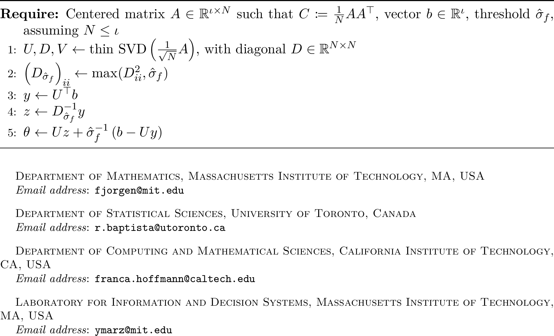
5.7 Auxiliary Results for Section 4.2.2↩︎
In this section, we give a proof of Lemma [lem:smf95satisfies95assumptions], which we restate here first. Some of the constants for the guarantees on the map \(T_y^{\text{SM},\mu}\) are given in Table [tbl:tab:smf95constants95values]. We split the proof of this lemma into three forthcoming results:
Assumption (1a) is established in Lemma 7.
Assumption (1b) is shown in Proposition 11.
Assumption (3) is proved in Lemma 8.
Lemma 7. Suppose Assumption 3 holds. Let \(\mu \in \mathcal{P}_2\left(\mathbb{R}^n\times\mathbb{R}^m\right)\). For any \(y^\star \in \mathbb{R}^m\), the map \(T^{\text{SM},\mu}_{y^\star}: \mathbb{R}^n \times \mathbb{R}^m \rightarrow \mathbb{R}^n\) is Lipschitz-continuous with constant \[\tilde{L}^\mu = \tilde{C}_\text{II}^\text{SM}\left(1 + \text{Tr}\mathrm{Cov}(\mu)^{\tilde{e}_{\text{II}}^\text{SM}}\right),\] where \[\tilde{C}_{\text{II}}^\text{SM} = \sqrt{n}2^{n-1} \left({2}^{n/2} + 4^n\hat{\sigma}_f^{-n}L_f^{2n}\right),\quad \tilde{e}_{\text{II}}^\text{SM} = n.\]
Proof. Fix \(x, x^\prime\in\mathbb{R}^n, y, y', y^\star \in \mathbb{R}^m\) and let \(w = T^{\text{SM},\mu}_{y^\star}(x,y), w '= T^{\text{SM},\mu}_{y^\star}(x',y')\). By definition of Equation 48 , we have the recursion \[w_k = x_k - \theta_k^\top\left(f_k(x,y) -f_k(w,y^\star)\right)\] with \(\theta_k \mathrel{\vcenter{:}}= \mathrm{Cov}_{\hat{\sigma}_f}\left( f_k( X, Y) \right)^{-1} \mathrm{Cov}\left( f_k( X, Y), X_k \right)\) and \((X,Y) \sim \mu\). Therefore, \[\begin{align} |w_k - w_k'|^2 &= \left|x_k - x_k' - \theta_k^\top\left(f_k(x,y) - f_k(x',y') -(f_k(w,y^\star) - f_k(w',y^\star)) \right) \right|^2\\ &\leq 2 \left|x_k - x_k'\right|^2 +4 \|\theta_k\|_2^2\Bigl( \left\|f_k(x,y) - f_k(x',y')\right\|^2_2\\ &\qquad\qquad + \left\|f_k(w,y^\star) - f_k(w',y^\star) \right\|^2_2\Bigr)\\ &\leq 2 \left|x_k - x_k'\right|^2 +4 \|\theta_k\|_2^2L_f^2\Bigl( \left\|(x_{1:k-1},y) - (x_{1:k-1}',y')\right\|^2_2\\ &\qquad\qquad + \left\|w_{1:k-1} - w_{1:k-1}' \right\|^2_2\Bigr), \end{align}\] where the last inequality follows from \(f_k\) being \(L_f\)-Lipschitz. Let \(\Delta_{1:k}^2 := \|w_{1:k} - w_{1:k}'\|_2^2\) and \(\tilde{\Delta}^2 := \|(x,y) - (x',y')\|_2^2\). Then, another upper bound for the result above implies the recursion: \[\begin{align} \Delta_{1:k}^2 \leq \left(2 + 4 \|\theta_k\|_2^2L_f^2\right)\tilde{\Delta}^2 + \left(2 + 4 \|\theta_k\|_2^2L_f^2 \right)\Delta_{1:k-1}^2 \end{align}\] The solution to this recursion is \[\begin{align} \Delta_{1:k}^2 & \leq \tilde{\Delta}^2\sum\limits_{\ell = 1}^k \left(\prod\limits_{g =\ell}^{k}\left(2 + {4\left\| \theta_g\right\|_2^2 L_f^2} \right)\right) \\ & \leq \tilde{\Delta}^2 k \prod\limits_{g =1}^{k}\left(2 + {4\left\| \theta_g\right\|_2^2 L_f^2} \right). \end{align}\] Finally, we need to bound \(\|\theta_k\|_2^2\). By applying Cauchy-Schwarz and bounding the change in moments under the pushforward of Lipschitz transformations, we have \[\begin{align} \left\|\theta_k \right\|_2^2& = \left\|\mathrm{Cov}_{\hat{\sigma}_f}\left( f_k( X, Y) \right)^{-1} \mathrm{Cov}\left( f_k( X, Y), X_k \right)\right\|_2^2 \nonumber \\ & \leq \hat{\sigma}_f^{-2}\left\|\mathrm{Cov}\left( f_k( X, Y), X_k \right) \right\|_2^2 \nonumber \\ & \leq 4\hat{\sigma}_f^{-2}L_f^2 \text{Tr}\mathrm{Cov}(\mu)^2. \label{eq:theta95k95norm95bound} \end{align}\tag{54}\] Therefore, applying Jensen’s inequality repeatedly results in the following upper bound for the Lipschitz constant: \[\begin{align} \frac{\Delta_{1:n}}{\tilde{\Delta}} &\leq \sqrt{n} \sqrt{\prod\limits_{g = 1}^n\left(2 + 16\hat{\sigma}_f^{-2}L_f^4 \text{Tr}\mathrm{Cov}(\mu)^2\right)} \\ & \leq \sqrt{n} {\left(\sqrt{2} + 4\hat{\sigma}_f^{-1}L_f^{2} {\text{Tr}\mathrm{Cov}(\mu)}\right)^n} \\ & \leq \sqrt{n}2^{n-1} \left({2}^{n/2} + 4^n\hat{\sigma}_f^{-n}L_f^{2n} \text{Tr}\mathrm{Cov}(\mu)^{n}\right)\\ & \leq \sqrt{n}2^{n-1} \left({2}^{n/2} + 4^n\hat{\sigma}_f^{-n}L_f^{2n}\right)\left(1+ \text{Tr}\mathrm{Cov}(\mu)^{n}\right). \end{align}\] ◻
Lemma 8. Suppose Assumption 3 holds. Let \(\mu \in \mathcal{P}_2\left(\mathbb{R}^n\times\mathbb{R}^m\right)\). Then, for any \(x\in\mathbb{R}^n, y,y^\star \in \mathbb{R}^m\) we have \[\left\|x - T^{\text{SM},\mu}_{y^\star}(x,y)\right\|_2 ^2 \leq n2^{n-1}\bigl(1 + 4^nL_f^{4n}\hat{\sigma}_f^{-2n} \text{Tr}\mathrm{Cov}(\mu)^{2n}\bigr) \left\|y - y^\star\right\|_2^2.\]
Proof. Let \[\theta_k \mathrel{\vcenter{:}}= \mathrm{Cov}_{\hat{\sigma}_f}\left( f_k( X, Y) \right)^{-1} \mathrm{Cov}\left( f_k( X, Y), X_k \right)\] for \((X, Y) \sim \mu\). Define \(w = T^{\text{SM},\mu}_{y^\star}(x,y)\). By definition from Equations 48 and 50 , for all \(k \geq 1\): \[\begin{align} \left|x_k - w_k\right|^2 & = \left| \theta_k^\top (f_k(x,y) - f_k(w, y^\star))\right|^2 \\ &\leq L_f^2\left\|\theta_k\right\|_2^2\left( \left\|x_{1:k-1} - w_{1:k-1}\right\|_2^2 +\|y - y^\star\|_2^2\right). \end{align}\] This shows inductively that \[\left\|x_{1:k} - w_{1:k}\right\|_2^2 \leq \left\|y - y^\star\right\|_2^2\sum\limits_{\ell = 1}^k \prod\limits_{g = \ell}^k (1 + L_f^2\left\|\theta_g\right\|_2^2).\] We can further bound this using elementary inequalities and Equation 54 as \[\begin{align} \left\|x - T^{\text{SM},\mu}_{y^\star}(x,y)\right\|_2^2 & \leq \left\|x_{1:n} - w_{1:n}\right\|_2^2 \\ &\leq n\left\|y - y^\star\right\|_2^2 \prod\limits_{g = 1}^n (1 + L_f^2\left\|\theta_g\right\|_2^2) \\ &\leq n\left\|y - y^\star\right\|_2^2 (1 + 4L_f^4\hat{\sigma}_f^{-2} \text{Tr}\mathrm{Cov}(\mu)^2)^n \\ &\leq n2^{n-1}\bigl(1 + 4^nL_f^{4n}\hat{\sigma}_f^{-2n} \text{Tr}\mathrm{Cov}(\mu)^{2n}\bigr) \left\|y - y^\star\right\|_2^2 \end{align}\] ◻
Lemma 9. Consider the Frobenius-projection defined in Equation 49 for a fixed \(\upsilon \geq0\). Then for symmetric matrices \(A, B \in \mathbb{R}^{u \times u}\), the projection \(A \mapsto A_\upsilon\) is a Lipschitz function in the Frobenius norm. That is, \[\|A_{\upsilon} - B_{\upsilon}\|_F \leq \|A - B\|_F.\]
Proof. By definition, \[A_\upsilon =\mathop{\mathrm{arg\,min}}_{\tilde{A} \succeq \upsilon I_{u}} f_{A}(\tilde{A}), \qquad f_A(\tilde{A}) \mathrel{\vcenter{:}}=\frac{1}{2}\left\|\tilde{A} - A\right\|_F^2.\] Let \(\langle\cdot,\cdot\rangle\) be the inner product inducing the Frobenius norm, i.e., \[\langle A, B\rangle \mathrel{\vcenter{:}}= \sum_{i,j=1}^u A_{ij}B_{ij}.\] This is a convex problem with \(f_A\) convex and differentiable. Moreover, the set of matrices \(\{\tilde{A} \in \mathbb{R}^{u \times u}: \tilde{A} \succeq \upsilon I_{u}\}\) where the optimization is performed is convex. Thus, by Equation 4.21 of [52], the KKT conditions give the following optimality criterion: \[\langle\nabla_{\tilde{A}}f_{A} (A_\upsilon), \tilde{A}-A_\upsilon\rangle = \langle A_\upsilon - A, \tilde{A}-A_\upsilon\rangle \geq 0 \text{ for all }\tilde{A}\succeq \upsilon I_u.\] Similarly, \[\langle B_\upsilon - B, \tilde{B}-B_\upsilon\rangle \geq 0 \text{ for all }\tilde{B}\succeq \upsilon I_u.\] In particular, \[\langle A_\upsilon - A, B_\upsilon-A_\upsilon\rangle \geq 0 ,\qquad \langle B_\upsilon - B, A_\upsilon-B_\upsilon\rangle \geq 0.\] Adding these together gives \[\langle A_\upsilon - B_\upsilon, B_\upsilon-A_\upsilon\rangle + \langle B - A, B_\upsilon-A_\upsilon\rangle \geq 0 \Leftrightarrow \langle B - A, B_\upsilon-A_\upsilon\rangle \geq \|A_\upsilon - B_\upsilon\|_F^2.\] The result then follows from Cauchy-Schwarz. ◻
Proposition 11. Suppose Assumption 3 holds. Let \(\mu, \nu \in \mathcal{P}_{2}\left(\mathbb{R}^n\times\mathbb{R}^m\right)\). Then, for any \(y^\star,y \in \mathbb{R}^m, x \in \mathbb{R}^n\) the mean-field stochastic map approximate conditioning map satisfies \[\begin{align} &\left\| T^{\text{SM},\mu}_{y^\star}(x,y) - T^{\text{SM},\nu}_{y^\star}(x,y)\right\|_2\\ &\quad \leq \tilde{C}_{\text{est}, \text{II}} \left(1 + \text{Tr}\mathrm{Cov}( \mu)^{2n+1} + \text{Tr}\mathrm{Cov}( \nu)^{2n+1} \right) \left\|y^\star - y\right\|_2 \\ &\qquad\cdot\left\|\mathrm{Cov}(g_\sharp\mu) - \mathrm{Cov}(g_\sharp\nu)\right\|_2 \end{align}\] for a constant \(\tilde{C}_{\text{est}, \text{II}} = \tilde{C}_{\text{est}, \text{II}}(n, b, L_f, \hat{\sigma}_f)\).
Proof. Let \[\begin{align} \theta_k &\mathrel{\vcenter{:}}= \mathrm{Cov}_{\hat{\sigma}_f}\left( f_k( X, Y) \right)^{-1} \mathrm{Cov}\left( f_k( X, Y), X_k \right) \\ \theta_k' &\mathrel{\vcenter{:}}= \mathrm{Cov}_{\hat{\sigma}_f}\left( f_k( X', Y') \right)^{-1} \mathrm{Cov}\left( f_k( X', Y'), X_k '\right) \end{align}\] for \((X, Y) \sim \mu, ( X', Y') \sim \nu\). Further, let \[w = T^{\text{SM},\mu}_{y^\star}(x,y), \qquad w' = T^{\text{SM},\nu}_{y^\star}(x,y).\] By definition from Equations@eq:eq:sm95approximate95conditioning95recursion and 50 , we have \[\begin{align} \left|w_k - w_k'\right|^2 & = \left|\theta_k^\top\left(f_k(x,y) -f_k(w,y^\star)\right) - \theta_k'^\top\left(f_k(x,y) -f_k(w',y^\star)\right) \right|^2\\ & = \left|\theta_k^\top\left(f_k(x,y) -f_k(x, y^\star) + f_k(x,y^\star)- f_k(w,y^\star)\right)\right. \\ &\left.- \theta_k'^\top\left(f_k(x,y) -f_k(x, y^\star) + f_k(x,y^\star) -f_k(w',y^\star)\right) \right|^2\\ & = \left|(\theta_k-\theta_k')^\top\left(f_k(x,y) -f_k(x, y^\star)\right)\right. \\ &\qquad\left. + (\theta_k -\theta_k')^\top(f_k(x,y^\star)- f_k(w,y^\star))\right. \\ & \left.- \theta_k'^\top\left(f_k(w,y^\star) -f_k(w',y^\star)\right) \right|^2\\ & \leq 3\Bigl(\|\theta_k -\theta_k'\|_2^2 \left(\|f_k(x,y) - f_k(x,y^\star)\|_2^2 + \|f_k(x,y^\star) - f_k(w,y^\star)\|_2^2 \right)\\ &\qquad + \|\theta_k'\|_2^2\|f_k(w,y^\star) - f_k(w',y^\star)\|_2^2\Bigr)\\ & \leq 3L_f^2\Bigl(\|\theta_k -\theta_k'\|_2^2 \left(\|y-y^\star\|_2^2 + \|x - w\|_2^2\right)\\ &\qquad + \|\theta_k'\|_2^2\|w_{1:k-1}-w'_{1:k-1}\|_2^2\Bigr). \end{align}\] Plugging in Lemma 8 and defining \(\Delta_{1:k}^2 = \|w_{1:k} - w_{1:k}'\|_2^2\), this yields \[\begin{align} \Delta_{1:k}^2 &\leq 3L_f^2\|\theta_k -\theta_k'\|_2^2 \left(1 + n2^{n-1}(1 + 4^nL_f^{4n}\hat{\sigma}_f^{-2n} \text{Tr}\mathrm{Cov}(\mu)^{2n}) \right) \|y-y^\star\|_2^2 \\ &\quad+\left(1 + 3L_f^2\|\theta_k'\|_2^2\right)\Delta_{1:k-1}^2 \end{align}\] Further, applying Equation 54 to \(\theta_k'\) with \((X',Y')\sim\nu\) shows \[\begin{align} \Delta_{1:k}^2 &\leq 3L_f^2\|\theta_k -\theta_k'\|_2^2 \left(1 + n2^{n-1}(1 + 4^nL_f^{4n}\hat{\sigma}_f^{-2n} \text{Tr}\mathrm{Cov}(\mu)^{2n}) \right) \|y-y^\star\|_2^2 \\ &\quad+\left(1 + 12L_f^4\hat{\sigma}_f^{-2} \text{Tr}\mathrm{Cov}(\nu)^2\right)\Delta_{1:k-1}^2. \end{align}\] Letting \[\begin{align} C_1& =3L_f^2\max_{1\leq k\leq n}\|\theta_k -\theta_k'\|_2^2 \left(1 + n2^{n-1}(1 + 4^nL_f^{4n}\hat{\sigma}_f^{-2n} \text{Tr}\mathrm{Cov}(\mu)^{2n}) \right) \|y-y^\star\|_2^2 \\ C_2& = \left(1 + 12L_f^4\hat{\sigma}_f^{-2} \text{Tr}\mathrm{Cov}(\nu)^2\right), \end{align}\] this shows inductively that \[\Delta_{1:n}^2 \leq \sum\limits_{\ell = 1}^n C_2^{n-\ell} C_1 \leq n C_1 C_2^n.\] Now, we bound \[\begin{align} \|\theta_k -\theta_k'\|_2^2 &= \left\| \mathrm{Cov}_{\hat{\sigma}_f}\left( f_k( X, Y) \right)^{-1} \mathrm{Cov}\left( f_k( X, Y), X_k \right) \right.\\ &\left.- \mathrm{Cov}_{\hat{\sigma}_f}\left( f_k( X', Y') \right)^{-1} \mathrm{Cov}\left( f_k( X', Y'), X_k' \right)\right\|_2^2\\ &\leq 2\left\| \mathrm{Cov}_{\hat{\sigma}_f}\left( f_k( X, Y) \right)^{-1} \mathrm{Cov}\left( f_k( X, Y), X_k \right) \right.\\ &-\left. \mathrm{Cov}_{\hat{\sigma}_f}\left( f_k( X, Y) \right)^{-1} \mathrm{Cov}\left( f_k( X', Y'), X_k' \right)\right\|_2^2 \\ &+2\left\| \mathrm{Cov}_{\hat{\sigma}_f}\left( f_k( X, Y) \right)^{-1} \mathrm{Cov}\left( f_k( X', Y'), X_k' \right)\right.\\ &-\left. \mathrm{Cov}_{\hat{\sigma}_f}\left( f_k( X', Y') \right)^{-1} \mathrm{Cov}\left( f_k( X', Y'), X_k' \right)\right\|_2^2 \\ &\leq 2\hat{\sigma}_f^{-2} \left\| \mathrm{Cov}\left( f_k( X, Y), X_k \right) - \mathrm{Cov}\left( f_k( X', Y'), X_k' \right)\right\|_2^2 \\ &+2\left\|\mathrm{Cov}\left( f_k( X', Y'), X_k' \right)\right\|_2^2\left\|\mathrm{Cov}_{\hat{\sigma}_f}\left( f_k( X, Y) \right)^{-1}\right.\\ &\left. \cdot \left(\mathrm{Cov}_{\hat{\sigma}_f}\left( f_k( X, Y) \right) - \mathrm{Cov}_{\hat{\sigma}_f}\left( f_k( X', Y') \right)\right) \mathrm{Cov}_{\hat{\sigma}_f}\left( f_k( X', Y') \right)^{-1} \right\|_2^2 \\ &\leq 2\hat{\sigma}_f^{-2} \left\| \mathrm{Cov}\left( f_k( X, Y), X_k \right) - \mathrm{Cov}\left( f_k( X', Y'), X_k' \right)\right\|_2^2 \\ &\quad+2\hat{\sigma}_f^{-4} \left\|\mathrm{Cov}\left( f_k( X', Y'), X_k' \right)\right\|_2^2\\ &\qquad\cdot \left\|\mathrm{Cov}_{\hat{\sigma}_f}\left( f_k( X, Y) \right) - \mathrm{Cov}_{\hat{\sigma}_f}\left( f_k( X', Y') \right) \right\|_2^2. \end{align}\] Set \[D_g\mathrel{\vcenter{:}}= \left\| \mathrm{Cov}\left( g( X, Y)\right) - \mathrm{Cov}\left( g( X', Y') \right)\right\|_2.\] Invoking Lemma 9, we find the following results: \[\begin{align} &\left\|\mathrm{Cov}_{\hat{\sigma}_f}\left( f_k( X, Y) \right) - \mathrm{Cov}_{\hat{\sigma}_f}\left( f_k( X', Y') \right) \right\|_2^2\\ &\qquad \leq \left\|\mathrm{Cov}_{\hat{\sigma}_f}\left( f_k( X, Y) \right) - \mathrm{Cov}_{\hat{\sigma}_f}\left( f_k( X', Y') \right) \right\|_F^2 \\ &\qquad \leq \left\|\mathrm{Cov}\left( f_k( X, Y) \right) - \mathrm{Cov}\left( f_k( X', Y') \right) \right\|_F^2 \\ &\qquad \leq bD_g^2.\\ &\left\| \mathrm{Cov}\left( f_k( X, Y), X_k \right) - \mathrm{Cov}\left( f_k( X', Y'), X_k' \right)\right\|_2^2\\ &\qquad \leq D_g^2. \end{align}\] Moreover, \[\left\|\mathrm{Cov}\left( f_k( X', Y'), X_k' \right)\right\|_2^2 \leq 2(L_f^2 + 1)^2\text{Tr}\mathrm{Cov}(\nu)^2.\] Thus, it follows that \[\begin{align} \|\theta_k -\theta_k'\|_2^2 &\leq C_3 \left(1 + \text{Tr}\mathrm{Cov}( \mu) + \text{Tr}\mathrm{Cov}(\nu)\right)^2 D_g^2 \end{align}\] for \(C_3 \mathrel{\vcenter{:}}= 2\hat{\sigma}_f^{-2}+4b(L_f^2 + 1)^2\hat{\sigma}_f^{-4}\). Plugging into \(\Delta_{1:n}^2\), we showed \[\begin{align} \Delta_{1:n}^2 &\leq n \left(1 + 12L_f^4\hat{\sigma}_f^{-2} \text{Tr}\mathrm{Cov}(\nu)^2\right)^n 3L_f^2\|\theta_k -\theta_k'\|_2^2\\ & \cdot \left(1 + n2^{n-1}(1 + 4^nL_f^{4n}\hat{\sigma}_f^{-2n} \text{Tr}\mathrm{Cov}(\mu)^{2n}) \right)\|y-y^\star\|_2^2 \\ & \leq C_4\left(1 + \text{Tr}\mathrm{Cov}(\mu)^{2n}\right) \left(1 + \text{Tr}\mathrm{Cov}(\nu)^{2n}\right) \|y-y^\star\|_2^2\|\theta_k -\theta_k'\|_2^2\\ &\leq C_3C_4\left(1 + \text{Tr}\mathrm{Cov}(\mu)^{2n}\right) \left(1 + \text{Tr}\mathrm{Cov}(\nu)^{2n}\right)\\ &\quad\cdot \|y-y^\star\|_2^2 \left(1 + \text{Tr}\mathrm{Cov}( \mu) + \text{Tr}\mathrm{Cov}(\nu)\right)^2 \\ & \cdot D_g^2 \\ &\leq C_5 \|y-y^\star\|_2^2 \left(1 + \text{Tr}\mathrm{Cov}( \mu)^{2n+1} + \text{Tr}\mathrm{Cov}(\nu)^{2n+1}\right)^2\\ &\cdot D_g^2, \end{align}\] where we defined the intermediary constant \[\begin{align} C_4 &\mathrel{\vcenter{:}}= 3L_f^2n2^{n-1} \left(1 + 12^nL_f^{4n}\hat{\sigma}_f^{-2n} \right)\\ &\quad\cdot \left(1 + n2^{n-1}(1 + 4^nL_f^{4n}\hat{\sigma}_f^{-2n}) \right), \end{align}\] and \(C_5 = C_5(n,b,L_f,\hat{\sigma}_f)\) absorbs \(C_3C_4\) and the polynomial bound in \(\text{Tr}\mathrm{Cov}(\mu)\) and \(\text{Tr}\mathrm{Cov}(\nu)\). Taking the square root gives the final result. ◻
References↩︎
For the observation model in Equation 2 with independent noise, the covariance of the \(Y\)-marginal is given by \(\mathrm{Cov}(\pi_Y) = \mathrm{Cov}(h_{\sharp}\pi_X) + \mathrm{Cov}(\nu_\eta^j)\) where \(\mathrm{Cov}(h_{\sharp}\pi_X)\) is the predictive covariance of \(Y\) induced by \(h\) and \(\pi_X\) and \(\mathrm{Cov}(\nu_\eta^j)\) is the observation-noise covariance at time \(j\). We will analyze the EnKF map with this form of the marginal covariance \(\mathrm{Cov}(\pi_Y)\) in Subsection 4.1.↩︎