Competitive satellite placement and the geography of orbital risk: evidence from the geostationary arc
June 24, 2026
Abstract
Some orbital locations are crowded while others remain unoccupied. We explain why using the geostationary orbit as a near-ideal laboratory: a mature, one-dimensional orbit in which satellite operators compete for position under first-come first-served allocation rules. Using the complete ITU registry and a simple competitive entry model, we predict the observed distribution of active GEO satellites with \(R^2 = 0.64\). In walk-forward tests, the structural model also predicts individual slot choices out of sample better than a fitted conditional-logit discrete-choice model. Our model also predicts the distribution of inactive payloads in GEO with \(R^2 = 0.44\), showing that the geography of debris risk can be predicted when it is a function of satellite launches. Surprisingly, we find that the current satellite distribution in GEO is relatively fair: driven by population rather than income and placing satellites in economically efficient locations. However, our model shows that this is only the case for mature slots.
1 Introduction↩︎
Some orbital locations are crowded while others remain empty. This is one of the most visible spatial patterns in space infrastructure, and one of the most consequential. In geostationary orbit, satellites cluster densely at some longitudes while large stretches of the same orbital ring remain lightly occupied. Understanding why this happens matters for slot allocation, spectrum coordination, and global communications coverage. It also matters for space sustainability, because debris accumulates as a result of satellite placements. If we can explain the geography of satellite deployment, we can begin to explain the geography of long-run orbital risk as well.
We study this question in geostationary orbit, a near-ideal laboratory for observing competitive location choice. GEO is physically one-dimensional: each longitude corresponds to a different footprint on Earth, and the value of that footprint depends on who lives below. The observed pattern is stark. Above Asia, Europe, and the Americas, multiple operators stack satellites at the same longitude. Above the central Pacific, sub-Saharan Africa, and Central Asia, the same ring remains comparatively empty. These are high-stakes decisions, made under ITU allocation rules and involving years of coordination and hundreds of millions of dollars per satellite.
Existing discussions of orbital debris usually begin after launch, with engineering models of collision, operation, disposal, and end-of-life behaviour. Those models are indispensable. But they leave open a prior question: how much of the future geography of congestion and debris is already encoded in where operators choose to locate in the first place? In GEO, that question can be tested directly. If competitive dynamics determine where active satellites concentrate, and inactive payloads accumulate where active satellites were placed, then a model of competitive entry should also contain information about the later distribution of debris. Existing models of the future orbital environment often project traffic from history rather than from a model of competitive placement—for example by repeating recent launches or extrapolating historical trends in launch traffic, explosions, and disposal practices [1], [2].
We argue that this pattern is governed by a simple logic of sequential competitive entry. On a one-dimensional orbit, operators position satellites to maximise market share under the ITU’s first-come, first-served allocation rules. Each entrant picks the slot that offers the largest share of unclaimed demand given the positions already taken. The result is path-dependent clustering: the earliest entrants lock in the highest-demand longitudes, and later entrants pile into the same crowded arcs because even a fractional share of a large market exceeds a full share of a thin one. GEO provides an unusually clean setting in which to test this mechanism because both the allocation rules and the spatial outcome are directly observable.
Using the ITU Compliance Assessment Monitor database, we show that a simple competitive entry model derived from GEO’s allocation rules—and using population as the driver of demand for satellite services—predicts the observed distribution of active satellites with \(R^2 = 0.64\). It reproduces the dense clusters above South and Southeast Asia, Europe, and the Americas, and the sparse coverage above the central Pacific and equatorial Africa. It also outperforms an income-based alternative: replacing population demand with GDP-weighted demand (also under competitive entry) reduces fit to \(R^2 = 0.11\). In walk-forward out-of-sample tests, the structural model predicts individual slot choices better than several specifications of a fitted conditional logit. In a 21-year forward simulation (\(N = 400\) genuine new entrants, 2000–2021), the model achieves \(R^2 = 0.35\) against a naive persistence baseline of \(R^2 = 0.09\), a fourfold improvement with no parameters fitted to slot-choice data. The same model also predicts the distribution of inactive payloads with \(R^2 = 0.44\), showing that a major orbital-risk pattern often treated as an engineering problem is partly downstream of the geography of entry itself.
The paper’s contribution goes beyond validating a model. We show that the uneven geography of orbital infrastructure is predictable from economic fundamentals, population geography, and physical constraints, and that this predictive power extends to the geography of debris accumulation. We demonstrate this in GEO, where the distribution of both active satellites and inactive payloads can be predicted by a model of competitive entry with no parameters fitted to slot-choice data. The broader implication is that wherever satellite deployment generates future debris, the spatial distribution of orbital risk will partly reflect the spatial pattern of competitive entry.
2 Results↩︎
2.1 A competitive entry model of orbital location↩︎
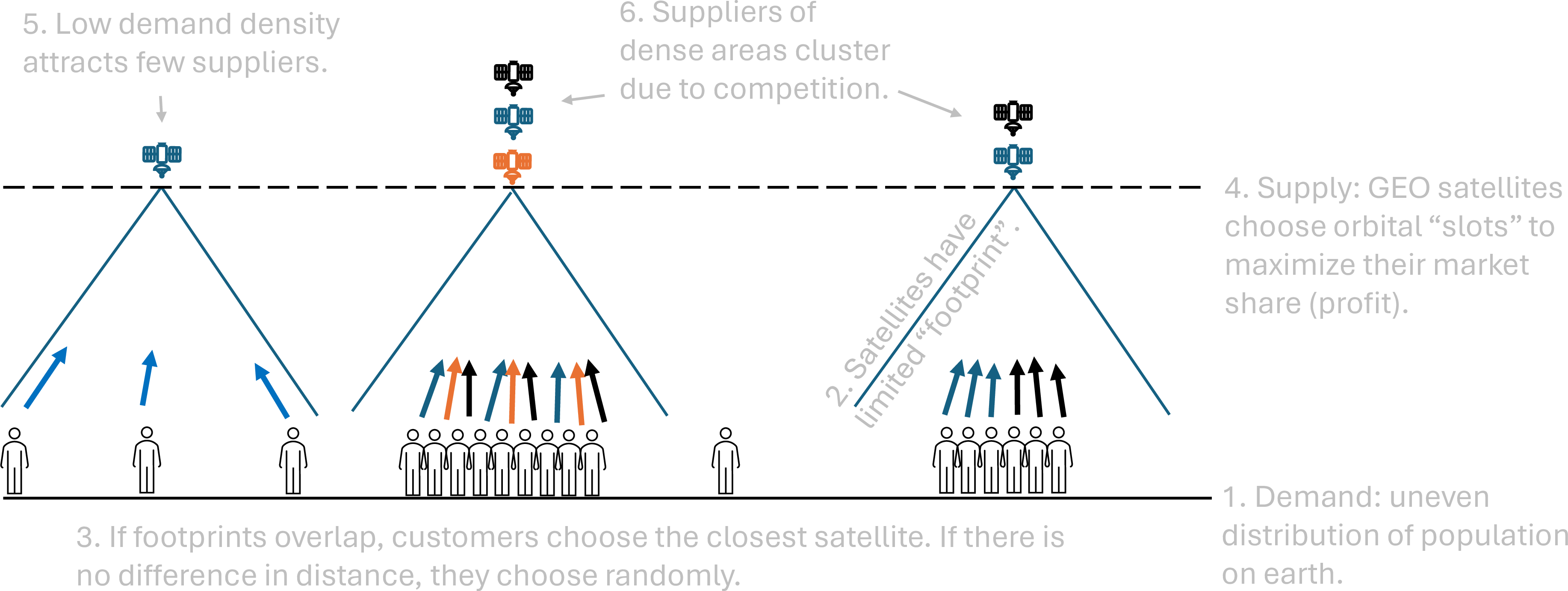
We model the geostationary belt as a ring of 360 positions, one per degree of longitude. From each position, a satellite serves the consumers within roughly \(40^\circ\) on either side—the effective commercial footprint of a GEO broadcast satellite—with each consumer’s demand going to the nearest satellite.3 The value of a position therefore depends on who lives within its footprint and how many competing satellites share it. Demand at each longitude is measured by gridded population [3].
Under the ITU’s first-come, first-served system, we model entry as a profit-maximising sequential process: each new operator picks the slot that maximises its own market share given the positions already occupied.
This process produces co-location—multiple satellites at the same longitude—through a simple path-dependent logic. The first entrant takes the highest-demand slot. Subsequent entrants face a trade-off: move to a less crowded but lower-demand location, or co-locate at a busy arc where demand is large enough to be shared. High-demand arcs attract entrant after entrant until the marginal gain from co-locating there falls below the payoff at the best remaining empty slot. Clustering is therefore the outcome of FCFS entry under heterogeneous demand, not a coordination failure. We find that clustering occurs because profit-maximising operators find it more advantageous to cluster at population peaks than to spread out. This concentration is a result of economic calculations, population geography, and physical constraints — not simply proportional demand-following.
2.2 The competitive entry model fits the observed distribution of active satellites↩︎
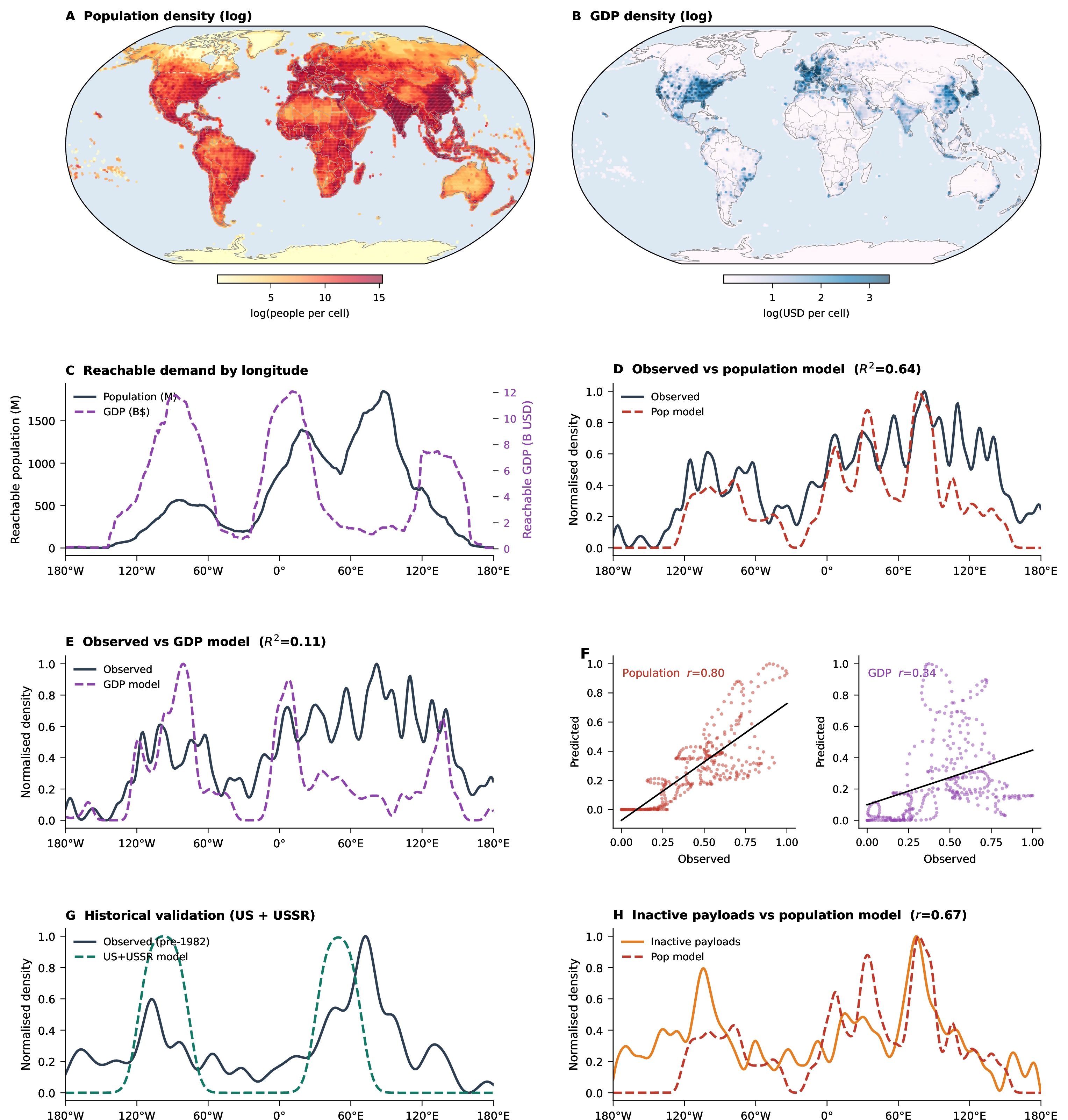
The CE model predicts the global distribution of active GEO satellites with \(R^2 = 0.64\) (Spearman \(\rho = 0.82\), K-S \(= 0.350\); Table 1). The geographic correspondence is visible in Figure 2: the model reproduces the dense clusters above South and Southeast Asia, Europe, and the Americas, and the sparse coverage above the central Pacific and equatorial Africa. A uniform baseline fails entirely (K-S \(= 0.997\)).
| \(R^2\) | K-S | MAE | Spearman \(\rho\) | |
|---|---|---|---|---|
| CE model, population demand (active satellites) | 0.64 | 0.350 | 0.179 | 0.82 |
| CE model, GDP demand (active satellites) | 0.11 | 0.397 | 0.274 | 0.51 |
| Uniform baseline | — | 0.997 | 0.441 | — |
| CE model, population demand (inactive payloads) | 0.44 | 0.256 | 0.164 | 0.61 |
| CE model, GDP demand (inactive payloads) | 0.01 | 0.378 | 0.258 | 0.20 |
2.3 Operators compete for population, not purchasing power↩︎
The model uses raw population as the demand measure. An alternative specification using GDP-weighted demand—income as a proxy for willingness to pay—fits substantially worse under the same competitive entry framework (\(R^2 = 0.11\), Spearman \(\rho = 0.51\); Table 1). The two measures differ most in Africa, the Middle East, and South Asia, where population is large relative to purchasing power; the population specification correctly predicts the dense concentration of satellites in the India arc, while the income-weighted alternative systematically misses it.
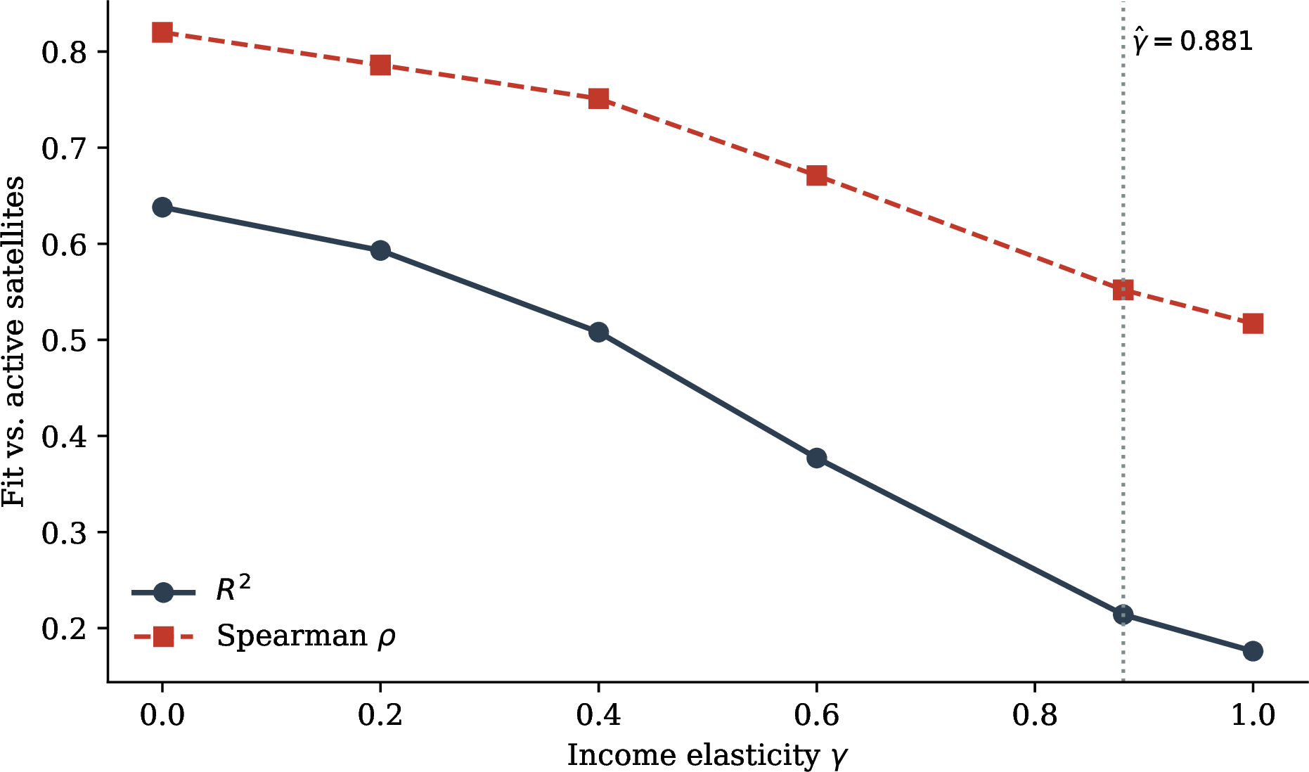
To test this more rigorously, we construct an income-adjusted demand measure and run it through the same competitive entry model as a robustness check. Specifically, we first estimate the income elasticity of satellite technology adoption independently from satellite placement data: using World Bank internet adoption rates across 192 countries (population-weighted WLS), we obtain \(\hat{\gamma} = 0.881\) (\(R^2 = 0.791\)) as the elasticity of technology adoption with respect to GDP per capita. We then scale each slot’s population demand by local GDP per capita raised to this power, and re-run the competitive entry model with this income-adjusted demand. This robustness check reduces fit from \(R^2 = 0.64\) to \(R^2 = 0.21\) (Appendix 7). The best-fitting income weight in the satellite data is \(\hat{\gamma} \approx 0\)—pure population. Any positive income weight deteriorates fit monotonically.
This finding has a specific implication for coverage equity. The coverage gaps in sub-Saharan Africa, Central Asia, and the Pacific persist not because those markets are unprofitable per subscriber, but because their populations are small relative to the global demand peaks that drive competitive clustering. Operators are not targeting wealthy consumers at the expense of poor ones; they are targeting population, and the geographic coincidence of large populations with moderate incomes explains the India arc concentration. This is a structural feature of competitive entry under heterogeneous demand, not a preference for wealth.
A rotation placebo test confirms that the population signal reflects longitude alignment specifically, not merely any lumpy predictor fitting a lumpy satellite map. We rotate the population distribution in \(5^\circ\) steps (72 rotations) and re-run the model for each rotation. The true alignment ranks first out of 61 rotations of \(\geq 30^\circ\) on both the logit McFadden \(R^2\) and the CE model Pearson \(r\) (empirical \(p = 1/62 \approx 1.6\%\); Appendix 6). An east–west mirror has essentially no predictive power (\(R^2 \approx 0.00002\), \(r \approx 0.01\)), confirming that the model requires not just the right amount of population but its correct east–west orientation.
A further check comes from the treatment of China. Chinese consumers face regulatory restrictions on receiving foreign satellite signals, so they are excluded from the demand measure—they do not form part of the addressable market for commercial GEO operators. When we instead include Chinese population, the model over-predicts the China arc and overall fit falls from \(R^2 = 0.638\) to \(R^2 = 0.633\) (Appendix 10). The direction is consistent with the addressable-market specification—including population that cannot purchase the service does not improve, and slightly worsens, the fit—though the difference is small, and we read this as a specification check rather than strong falsification evidence.
2.4 The model predicts satellite deployment out of sample↩︎
2.4.0.1 Slot-level walk-forward prediction.
We test whether the CE correctly predicts which of the 360 slots each individual satellite chose at launch, using the state of the orbit at launch as the information set. For each of the 431 post-2000 new-entry commercial satellites, we rank all 360 slots by their CE-predicted market share and record the rank of the slot that was actually chosen: rank 1 means the model predicted the chosen slot as the most profitable, rank 360 means it predicted it as least profitable, and a random predictor would achieve a mean rank of 180. In this walk-forward out-of-sample exercise—with no parameters fitted to slot-choice data—the CE model achieves a mean rank of 140 out of 360, outperforming a conditional logit fitted in-sample (mean rank 154; Appendix 5). The structural model, with no free parameters adjusted to match slot-choice data, beats the flexible fitted model out of sample. This is the standard signature of a correctly-specified structural model: it generalises where fitted models overfit.
2.4.0.2 Long-run deployment prediction (2000–2021).
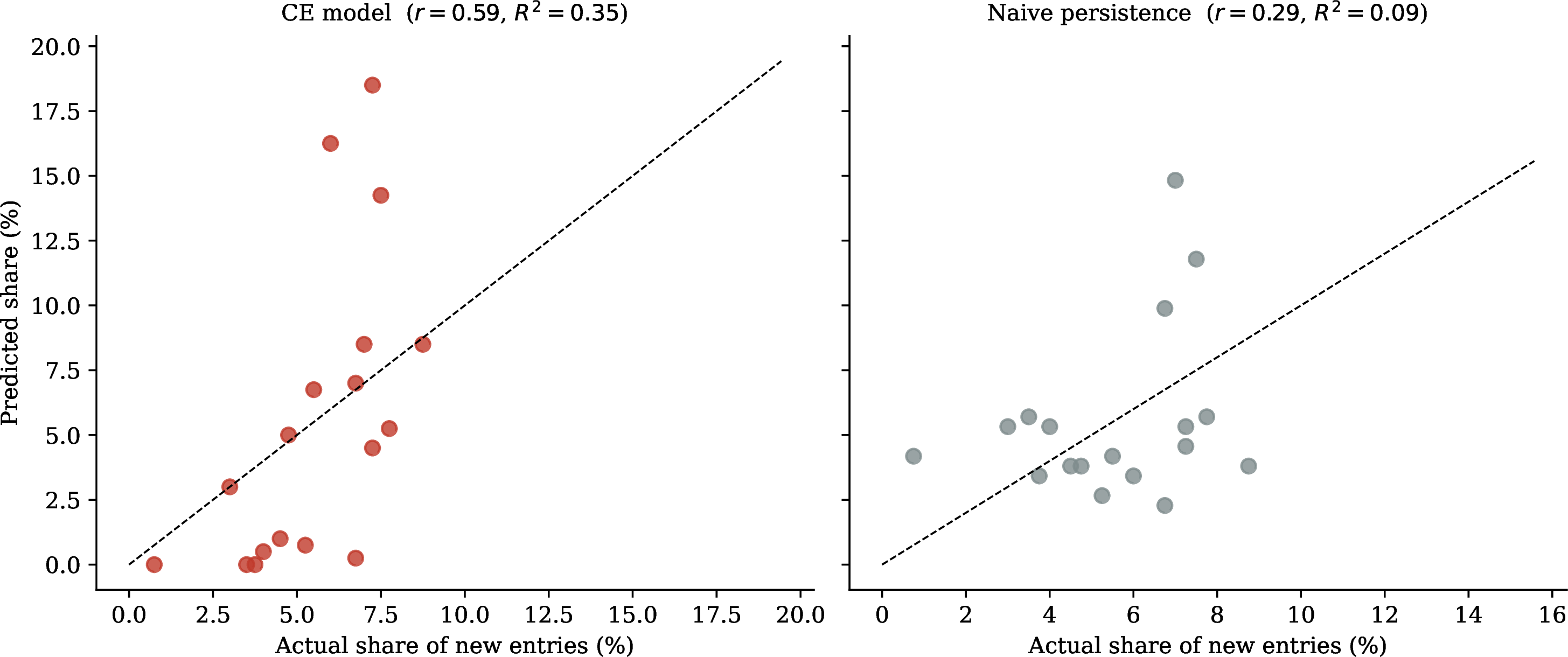
We conduct a more demanding test at the aggregate level. Starting from the satellites in orbit at end-2000, we run the CE model forward over the full subsequent 21-year period, placing 400 satellites—the number of genuine new slot-choice decisions made through 2021 after excluding the approximately 17% of launches that were strict replacements at the same operator’s existing slot (see Appendix 5). Comparing the predicted arc-level distribution of these entries (in \(20^\circ\) bins) to the actual 2000–2021 new-entry distribution, the CE achieves \(r = 0.59\), \(R^2 = 0.35\). A naive persistence benchmark—predicting new entries proportional to the 2000 distribution—achieves \(r = 0.292\), \(R^2 = 0.09\). The CE beats the naive benchmark by \(+0.30\) in Pearson correlation, a fourfold improvement in \(R^2\), despite using no data beyond the starting orbital configuration.
Two measurement challenges bear noting. For short-run slot-level predictions, the fact that a slot appears unoccupied in our data does not mean it is freely available: the ITU slot coordination process is complex and can take years, so some “empty” slots may already be under negotiation or reserved. For long-run aggregate predictions, identifying genuine new entries is imprecise because replacement launches—a satellite taking over its predecessor’s exact slot—are difficult to identify reliably in the registry data. Despite both challenges, the model beats its benchmarks at both horizons, confirming that the competitive entry mechanism captures something real about how operators choose locations.
2.5 The model predicts where debris will accumulate↩︎
Decommissioned satellites remain in orbit. When a satellite reaches end-of-life, it is either boosted to a graveyard orbit or remains near GEO, joining the growing population of inactive payloads that constitute a long-run debris hazard. If competitive dynamics drive active satellite placement, and inactive payloads accumulate where active satellites were placed, then the same model should predict the distribution of orbital debris.
We test this directly. Using the 513 inactive payloads in the ITU-CAM database, we compare their longitude distribution to the CE model’s prediction. The CE model achieves \(R^2 = 0.44\) for inactive payloads versus \(R^2 = 0.01\) for the GDP-based alternative (Table 1, Figure 2, panel H). The geographic pattern that drives active satellite clustering—population concentration above the India arc—also predicts where debris concentrates decades later, though more weakly than for the active fleet. The weaker fit is expected: inactive payloads accumulate over the full history of entry through end-of-life drift, station-keeping failure, and graveyard-orbit compliance—processes the CE model does not describe—so the comparison asks only whether the long-run CE geography also marks where earlier generations of satellites were left. Both distributions peak at the same high-demand arcs.
This result has a direct practical use. Current debris risk assessments rely on engineering models of individual satellite end-of-life behaviour. The CE model offers a complementary, pre-launch prediction: the longitudes that will be most congested with debris over the long run are precisely those that competitive dynamics will target with new satellites today. No engineering data is required. The regions at greatest long-run debris risk—the India arc, followed by Europe and the Americas—are exactly those where continued competitive entry will compound both congestion and debris.
3 Discussion↩︎
3.0.0.1 Sequential entry as the mechanism.
The GEO orbit is one of the rare arenas in which competitive location choice is physically one-dimensional, institutionally governed by explicit priority rules, and empirically observable in full. Our finding—\(R^2 = 0.64\) for the population-based competitive entry model versus \(R^2 = 0.11\) for the income-weighted alternative—confirms that the profit-maximising, path-dependent logic of FCFS entry explains the orbital distribution in the many-player, uneven-demand setting. The result matters because it shows that clustering is not an artefact of strategic forecasting or simultaneous optimisation, but emerges directly from the simple rule that each entrant picks the best available slot. This is important for understanding how allocation rules shape long-run spatial outcomes in resource competition more broadly.
3.0.0.2 Why the mechanism matters for orbital governance.
The CE model is not a description of the past alone—it is a predictive tool for the future. The competitive mechanism we document implies that new satellite systems will concentrate at the same longitudes that are already crowded, because profit-maximising entry makes dispersal individually costly. Three specific implications follow.
First, the population-over-income finding identifies which populations will remain underserved under competitive allocation and why. Coverage gaps in sub-Saharan Africa, Central Asia, and the Pacific are structural features of competitive entry under heterogeneous demand, predictable decades in advance. They will not close spontaneously as satellite technology matures.
Second, the debris prediction connects orbital competition to space sustainability. The longitudes most at risk from long-run debris accumulation are the same ones that competitive dynamics will continue to fill. This creates a self-reinforcing hazard: the most commercially attractive slots attract the most satellites, generate the most debris, and will eventually become the most operationally risky.
Third, the same mechanism is now playing out in low-Earth orbit (LEO) at an order of magnitude larger scale. Mega-constellation operators are filing for hundreds of thousands of satellites; the population-driven clustering logic predicts that their ground tracks will concentrate capacity above the same high-density regions that dominate GEO competition. Our model provides the first validated framework for anticipating where this concentration will occur, during the window when governance choices can still shape it.
3.0.0.3 Welfare and efficiency.
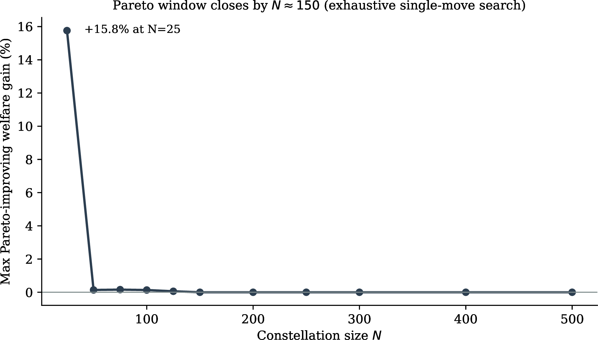
We find no evidence that the current orbit is inefficient in aggregate. We simply show that our model predicted that this would be the case at the early stages of populating the orbit: at \(N = 25\) satellites, a single reallocation could have improved consumer welfare by 15.8% while preserving every operator’s market share. This window closes quickly: from \(N = 50\) the best reallocation satisfying every operator’s participation constraint improves welfare by less than 0.2%, and from \(N \approx 150\)—including the current fleet size of \(N \approx 500\)—our exhaustive search finds no such reallocation at all. We deliberately do not map these constellation sizes to calendar dates: the early GEO era was dominated by the superpowers and the highly regulated Intelsat system, which lie outside the commercial competitive entry mechanism the model describes, so the model’s small-\(N\) counterfactual cannot be verified against the historical record.
3.0.0.4 Limitations.
The nearest-provider market sharing rule is a reduced-form approximation to actual subscription patterns; it is implemented identically throughout the analysis (arc distance, deterministic tie-breaking; Methods), and the replication package regenerates every number in this paper from a single implementation of the rule. Our entry mechanism also abstracts from the ITU coordination process: real slot assignments emerge from Appendix 30/30A/30B filing priority, multi-year coordination, and occasional state direction, of which first-come, first-served profit-maximising entry is a reduced form. The cross-sectional fit shows this reduced form has predictive content; it does not identify filing-level behaviour. We abstract from fleet-level optimisation, though Appendix 8 shows that a fleet marginal-gain model yields broadly consistent distributional patterns, confirming the finding is robust to alternative entry assumptions. The cross-sectional focus is deliberate: ITU filings record coordination requests years in advance, making the time-series of slot changes difficult to interpret as strategic choices; the cross-section aggregates over this noise and reflects the long-run outcome of competitive entry. Our temporal prediction test does not explicitly exclude Chinese-arc entries, and Chinese placement behaviour lies partly outside the commercial competition logic the model captures (Appendix 10).
4 Methods↩︎
4.1 Data↩︎
4.1.0.1 Satellite positions.
We use the ITU-CAM database [4]. Each satellite’s long-run average longitude is mapped to the nearest one-degree slot. Active satellites: \(N = 390\) post-2006 commercial and civil payloads (2006 is the first year for which the dataset provides near-complete commercial coverage, corresponding to the broad adoption of ITU filing requirements). Inactive payloads: \(N = 513\) decommissioned satellites. The replacement satellite filter (Appendix 5) excludes filings where the same operator already occupies the exact slot at the time of the new launch; approximately 13–22% of post-2000 satellites are strict replacements.
4.1.0.2 Population and income.
Population: Gridded Population of the World v4 (GPWv4) [3], 30 arc-second resolution, aggregated to \(1^\circ\) longitude strips, year 2005. Chinese population is excluded from the commercial demand distribution because Chinese consumers are restricted from accessing commercial satellite services (see Appendix 10). GDP per capita: G-Econ database version 4 [5], [6], year 2000.
4.1.0.3 Historical validation.
We validate the model against the early GEO constellation by simulating a “space-race” allocation using only US and Soviet populations as demand, placing 80 satellites to approximate the observed 1981 constellation. The model reproduces the density spikes observed around 60–120\(^\circ\)W (Americas) and 30–100\(^\circ\)E (Eurasian landmass; Figure 2, panel G). This exercise shows the model is consistent with the early constellation, not that it identifies the mechanism: a state-directed allocation placing each superpower’s satellites above its own territory would produce similar spikes from the same demand. The discriminating evidence for competitive entry comes from the commercial era. The US–USSR demand vector (GPWv4 2005 population of the United States and the Soviet successor states within the \(\pm 40^\circ\) latitude band) ships with the replication package.
4.2 CE computation↩︎
The CE is computed by profit-maximising sequential entry. Let \(\mathcal{S} = \{0,1,\ldots,359\}\) index slots and \(\mathrm{pop}_i\) denote population at slot \(i\). Starting from an empty arc (or a historical seed), each entrant \(k\) picks:
\[s_k = \arg\max_{s \in \mathcal{S}} T(s; \{s_1,\ldots,s_{k-1}\}),\]
where \(T(s;\,\cdot\,)\) is the market share accruing to a satellite at slot \(s\) given prior entrants—consumers go to the nearest satellite within \(\pm 40^\circ\), with ties split equally among tied satellites. Distance is arc (circular) distance, \(d(a,b) = \min(|a-b|,\, 360-|a-b|)\); among slots offering the entrant an equal market share, the lowest-numbered slot is chosen, making the placement sequence deterministic; at most six satellites may occupy one slot. The simulation places 700 entrants and the analysis uses the first 500, approximately the size of the current commercial fleet. Predicted densities in Table 1 and Figure 2 comprise the 80 space-race-era placements (simulated under US and Soviet demand; Section 4.1) followed by the 500 commercial-era placements, mirroring the two eras of GEO settlement. The reach radius (\(\pm 40^\circ\)), the per-slot capacity (6), and the fleet size (\(N = 500\)) are modelling choices set from engineering and institutional facts, not fitted to the satellite distribution. The algorithm runs in \(O(N \times 360^2)\) time and completes 500 placements in under 2 seconds. The CE with \(N = 500\) achieves \(R^2 = 0.64\).
4.3 Long-run deployment prediction↩︎
We take the actual satellite distribution at end-2000 as the starting state and run the CE algorithm forward, placing \(N = 400\) satellites corresponding to the genuine new slot-choice decisions made through 2021 (strict replacements excluded using the flag from Appendix 5). The predicted new-entry distribution is compared to the actual 2000–2021 new entries at \(20^\circ\) longitude bins using Pearson \(r\). The naive persistence benchmark predicts new entries proportional to the 2000 distribution.
4.4 Pareto efficiency test↩︎
For each constellation size \(N\), we compute the CE, record each satellite’s market share \(\pi_k^*\), and conduct an exhaustive search over all single-satellite reallocations, asking whether any reallocation \(\mathbf{n}'\) satisfies \(\pi_k(\mathbf{n}') \geq \pi_k^*\) for all \(k\) and raises aggregate consumer welfare \(W(\mathbf{n}') > W(\mathbf{n}^*)\), where \[W(\mathbf{n}) = \frac{\sum_i \mathrm{pop}_i \cdot q(s^*(i;\mathbf{n}),\,i)}{\sum_i \mathrm{pop}_i}, \quad q(s,i) = \max\!\left(0,\; 1 - \frac{d(s,i)}{R}\right), \label{eq:welfare}\tag{1}\] with \(d(\cdot,\cdot)\) the arc distance defined above. Each operator’s participation constraint \(\pi_k(\mathbf{n}') \geq \pi_k^*\) is evaluated under the same nearest-provider market-share rule and arc metric as the CE itself.
5 Conditional Logit Estimates and Slot-Choice Prediction↩︎
5.0.0.1 Setup.
For each of the 431 post-2000 new-entry commercial satellites, we construct a choice set of all 360 slots and compute: (i) population reach—population within \(\pm 40^\circ\), normalised by the mean; (ii) lagged occupancy—satellites already at the exact slot at launch; (iii) nearby occupancy—satellites within \(\pm 2^\circ\); (iv) own-operator prior—indicator for the operator already holding a satellite within \(\pm 2^\circ\). The conditional logit is estimated via L-BFGS-B maximum likelihood.
5.0.0.2 Replacement filter.
A satellite is classified as a strict replacement if the same operator already occupies the exact slot at launch. Strict replacements constitute approximately 13–22% of post-2000 commercial satellites, rising to 63% of launches in 2020 alone. Lagged occupancy flips from \(+0.064\) in the full sample to \(-0.051\) in the new-entry sample (post-2000, Specification 3): genuine new entrants avoid congested slots, consistent with competitive dynamics. All key results use the new-entry sample.
Table 2 reports all 16 specifications. Population reach is positive and significant across all specifications. The GDP-based alternative loses significance in the post-2000 new-entry sample, reinforcing the population-over-income finding.
| (1) Pop only | (2) +Occ | (3) +Own prior | (4) GDP | |||||
| Full | New entry | Full | New entry | Full | New entry | Full | New entry | |
| 2-3(lr)4-5(lr)6-7(lr)8-9 | ||||||||
| Population reach (norm.) | \(0.2588^{***}\) | \(0.2107^{***}\) | \(0.2212^{***}\) | \(0.2078^{***}\) | \(0.2207^{***}\) | \(0.2092^{***}\) | ||
| (0.0499) | (0.0537) | (0.0516) | (0.0552) | (0.0516) | (0.0552) | |||
| GDP reach (norm.) | \(0.1840^{**}\) | \(0.1483^{*}\) | ||||||
| (0.0786) | (0.0851) | |||||||
| Lagged occupancy (exact slot) | \(0.0989^{***}\) | -0.0230 | \(0.0771^{**}\) | -0.0286 | \(0.0901^{***}\) | -0.0173 | ||
| (0.0303) | (0.0365) | (0.0304) | (0.0365) | (0.0303) | (0.0365) | |||
| Nearby occupancy (\(\pm 2^\circ\)) | \(0.0277^{*}\) | 0.0100 | 0.0070 | 0.0046 | 0.0187 | 0.0164 | ||
| (0.0162) | (0.0182) | (0.0165) | (0.0183) | (0.0161) | (0.0179) | |||
| Own-operator prior presence | \(1.1930^{***}\) | \(0.3554^{***}\) | \(1.2081^{***}\) | \(0.3668^{***}\) | ||||
| (0.1085) | (0.1371) | (0.1081) | (0.1375) | |||||
| Observations | 667 | 580 | 667 | 580 | 667 | 580 | 667 | 580 |
| McFadden \(R^2\) | 0.0034 | 0.0022 | 0.0050 | 0.0023 | 0.0189 | 0.0033 | 0.0173 | 0.0016 |
| Panel B: Entry from 2000 onwards | ||||||||
| Population reach (norm.) | \(0.3570^{***}\) | \(0.3085^{***}\) | \(0.3159^{***}\) | \(0.3075^{***}\) | \(0.3156^{***}\) | \(0.3095^{***}\) | ||
| (0.0567) | (0.0619) | (0.0587) | (0.0638) | (0.0588) | (0.0638) | |||
| GDP reach (norm.) | \(0.1866^{**}\) | 0.1596 | ||||||
| (0.0898) | (0.0990) | |||||||
| Lagged occupancy (exact slot) | \(0.0877^{***}\) | -0.0445 | \(0.0643^{**}\) | -0.0510 | \(0.0822^{***}\) | -0.0354 | ||
| (0.0317) | (0.0387) | (0.0317) | (0.0388) | (0.0316) | (0.0389) | |||
| Nearby occupancy (\(\pm 2^\circ\)) | \(0.0297^{*}\) | 0.0116 | 0.0072 | 0.0051 | 0.0236 | 0.0219 | ||
| (0.0169) | (0.0191) | (0.0171) | (0.0192) | (0.0167) | (0.0187) | |||
| Own-operator prior presence | \(1.4118^{***}\) | \(0.4767^{***}\) | \(1.4215^{***}\) | \(0.4847^{***}\) | ||||
| (0.1195) | (0.1537) | (0.1187) | (0.1542) | |||||
| Observations | 513 | 431 | 513 | 431 | 513 | 431 | 513 | 431 |
| McFadden \(R^2\) | 0.0065 | 0.0048 | 0.0082 | 0.0052 | 0.0289 | 0.0069 | 0.0250 | 0.0029 |
| Notes: Conditional logit estimates. Each observation is one satellite; choice set = all 360 one-degree GEO slots. New entry columns exclude satellites where the same operator already occupied the exact same slot at the time of launch (strict replacement filter). Population reach is total population within \(\pm 40^\circ\) of slot, normalised by mean. Lagged occupancy counts satellites already at the slot. Nearby occupancy counts satellites within \(\pm 2^\circ\) (excluding exact slot). Own-operator prior equals one if the operator already holds a satellite within \(\pm 2^\circ\). Specification (4) replaces population with GDP-weighted reach. \(^{***}p<0.01\), \(^{**}p<0.05\), \(^{*}p<0.10\). | ||||||||
5.0.0.3 Out-of-sample prediction.
For each satellite, we rank all 360 slots by their model-predicted attractiveness and record the rank of the slot actually chosen (rank 1 = model’s top pick, rank 360 = model’s worst pick, random predictor mean = 180). Walk-forward OOS mean ranks (Table 3): CE model 140, conditional logit 154, random baseline 180. The structural model outperforms the fitted logit out of sample despite having no free parameters.
| Predictor | In-sample | Walk-forward OOS |
|---|---|---|
| Random baseline | 180 | 180 |
| CE model | 158 | 140 |
| Conditional logit (3) | 151 | 154 |
| Augmented logit | 149 | 158 |
| Post-2000 new-entry, \(N = 431\). Augmented logit adds \(\log(\text{CE market share})\) to Specification (3). | ||
5.0.0.4 Sequential convergence of the CE model.
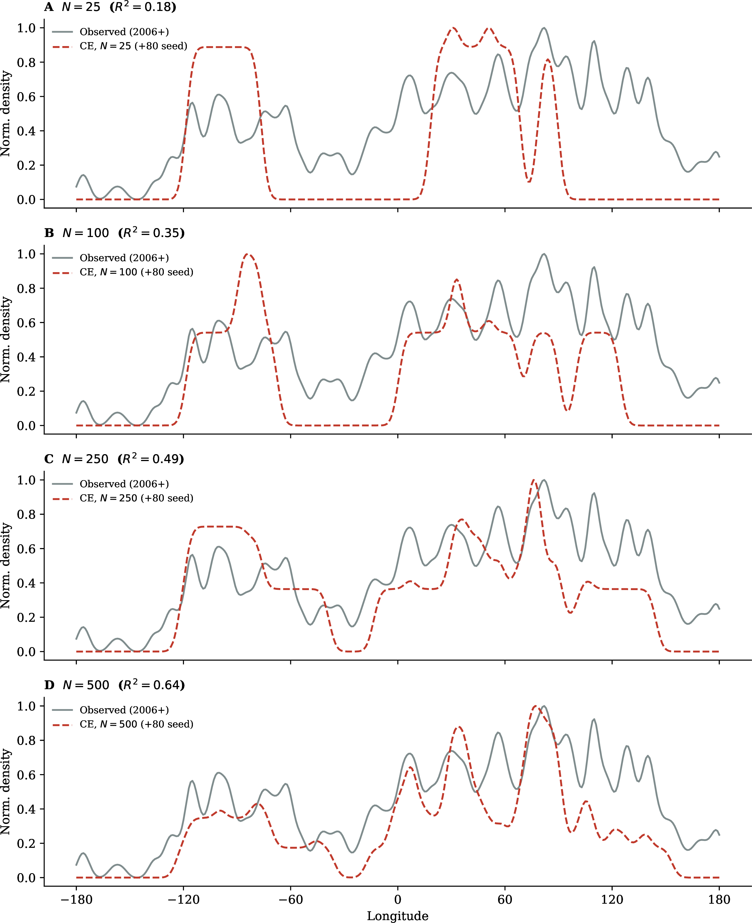
Figure 3 illustrates how the predicted distribution evolves as the number of profit-maximising entrants grows from \(N=25\) to \(N=500\). At small \(N\) the model already targets the highest-demand arcs; by \(N=250\) the broad shape of the observed distribution is reproduced; at \(N=500\) the prediction matches Figure 2 panel D exactly.
5.0.0.5 Long-run aggregate deployment prediction.
Figure 4 shows the aggregate long-run prediction at the \(20^\circ\)-arc level for the same fixed 2000–2021 window reported in the main text. Seeding from the 2000 constellation and placing 400 satellites forward, the CE model (\(R^2 = 0.35\)) substantially outperforms the naive persistence benchmark (\(R^2 = 0.09\)), which simply predicts new entries proportional to the 2000 distribution. The replication package also reports the full panel of alternative start and end years for transparency; all figures and statistics in the paper use the fixed 2000–2021 window.
6 Population Rotation Placebo Test↩︎
6.0.0.1 Method.
We rotate the longitude population distribution in \(5^\circ\) steps (72 rotations). Each rotation preserves total population, smoothness, and peak-to-trough structure; only the east–west alignment with actual orbit longitudes changes. For each rotation we (i) re-estimate the conditional logit (post-2000 new-entry, population reach only) and record McFadden \(R^2\); and (ii) re-run the CE model and record Pearson \(r\) against the actual slot distribution in \(20^\circ\) bins.
6.0.0.2 Results.
The true alignment (\(0^\circ\) rotation) ranks 1st of 61 rotations of \(\geq 30^\circ\) on both metrics (empirical \(p = 1/62 \approx 1.6\%\); Table 4, Figure 5). The east–west mirror has essentially no predictive power (\(R^2 \approx 0.00002\), \(r \approx 0.01\)): the distribution must be in the correct east–west orientation, not merely of the right magnitude.
| McFadden \(R^2\) | CE model \(r\) | |
|---|---|---|
| True alignment (\(0^\circ\)) | 0.00481 | 0.587 |
| Placebo mean (71 non-zero rotations) | 0.00124 | \(-0.022\) |
| True rank among \(\geq 30^\circ\) placebos | 1st/61 | 1st/61 |
| Mirror (east–west flip) | 0.00002 | 0.012 |

7 Income Elasticity and Mixed-Demand Robustness↩︎
7.0.0.1 Procedure.
This appendix applies an independently estimated income elasticity of technology adoption to the competitive entry model as a robustness check. The idea is to ask: if operators weighted their demand estimates by income (because wealthier consumers buy more satellite services), would the model fit better or worse?
We proceed in two steps. First, we estimate the income elasticity \(\gamma\) from cross-country data that are entirely independent of the satellite data. Using World Bank internet adoption rates across 192 countries (population-weighted WLS), we regress \(\log(\text{internet\%}_i)\) on \(\log(\text{GDP pc}_i)\), obtaining \(\hat{\gamma} = 0.881\) (\(R^2 = 0.791\)). This elasticity reflects how strongly technology adoption scales with income across countries.
Second, we apply this elasticity to the demand measure used in the competitive entry model. We construct income-adjusted demand \(\tilde{n}(s) = n(s) \times \bar{y}(s)^\gamma\), where \(\bar{y}(s)\) is GDP per capita at longitude \(s\) normalised by the global population-weighted mean. At \(\gamma = 0\) this collapses to the population baseline; at \(\gamma = 1\) it equals total GDP. We then re-run the competitive entry model using \(\tilde{n}(s)\) as the demand driver and compare the fit to the baseline.
7.0.0.2 Results.
Applying the externally estimated \(\hat{\gamma} = 0.881\) reduces CE model fit from \(R^2 = 0.64\) to \(R^2 = 0.21\) (Table 5). Fit declines monotonically with \(\gamma\) (Table 5, Figure 6): any positive income weight worsens prediction. The best-fitting elasticity in the satellite data is \(\hat{\gamma} \approx 0\)—pure population—and the externally estimated elasticity sharply worsens model performance. This confirms that operators target population concentration rather than purchasing power.
| \(\gamma\) | \(R^2\) | K-S | MAE | Spearman \(\rho\) |
|---|---|---|---|---|
| 0.0 (baseline) | 0.638 | 0.350 | 0.179 | 0.820 |
| 0.2 | 0.593 | 0.306 | 0.176 | 0.786 |
| 0.4 | 0.508 | 0.247 | 0.183 | 0.751 |
| 0.6 | 0.377 | 0.272 | 0.203 | 0.671 |
| 0.881 (estimated) | 0.214 | 0.322 | 0.230 | 0.552 |
| 1.0 (GDP only) | 0.176 | 0.342 | 0.237 | 0.517 |
| \(\hat\gamma = 0.881\) estimated from cross-country internet adoption; \(\gamma = 0\) replicates the main-text population baseline (\(R^2 = 0.64\), Table 1). Fit is measured at 1\(^\circ\) slots against \(N = 390\) active commercial satellites (v3 dataset, post-2006), consistent with the main analysis. | ||||
7.0.0.3 Coverage quality by income.
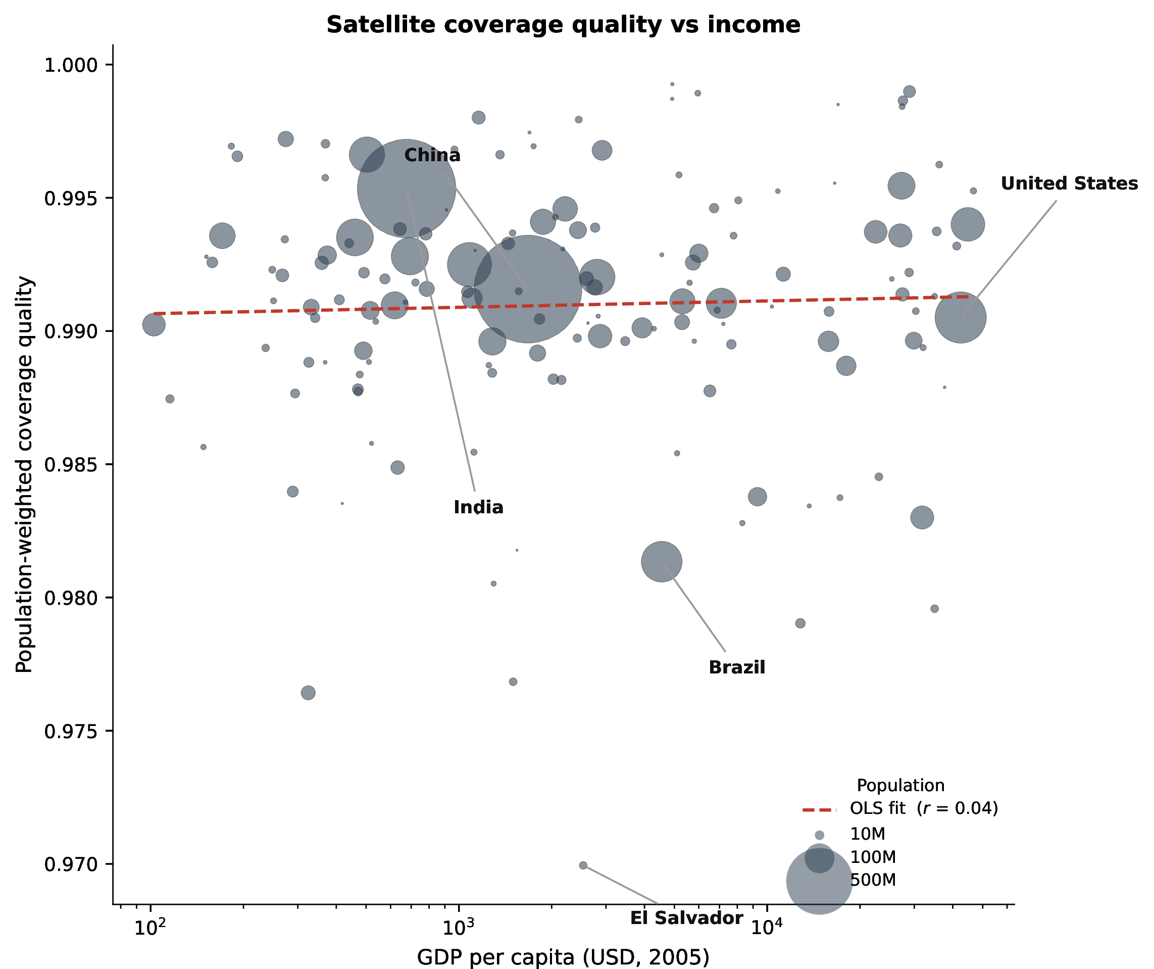
Figure 7 provides a complementary cross-country view. Despite the wide variation in GDP per capita across countries, coverage quality (the population-weighted proximity of each country to its nearest GEO satellite) shows little income gradient. This is consistent with the main finding: because operators target population peaks rather than purchasing power, even lower-income countries near dense arcs are relatively well served. The narrow \(y\)-axis range reflects that with \(\sim\)390 active satellites the ring is well populated; the variation that does exist is driven by geography, not income.
8 Fleet-Level Entry and Broadband Discount↩︎
8.0.0.1 Fleet-level entry.
Large operators manage multi-satellite portfolios. We implement a fleet marginal-gain model in which each satellite is placed to maximise the increment to its operator’s total territory: \(\Delta\pi_{\mathrm{fleet}}(s) = \sum_i \mathrm{pop}_i [\phi_i(s \cup E_k) - \phi_i(E_k)]\), where \(E_k\) is operator \(k\)’s existing fleet and \(\phi_i(E_k)\) is the fraction of consumer \(i\)’s demand captured by any satellite in \(E_k\). This reduces the K-S statistic relative to a flat-distribution baseline and the out-of-sample mean rank from 140.3 to 137.9.
8.0.0.2 Broadband discount.
Where terrestrial broadband is available, the satellite market is smaller. We discount slot-level demand by local broadband penetration: \(\tilde{n}(s) = n(s) \times \max(1 - b(s),\; 0.05)\), where \(b(s)\) is World Bank fixed broadband subscriptions per 100 people (2005), smoothed by Gaussian kernel (\(\sigma = 15^\circ\)). Global mean penetration in 2005 was 4.4%, so the effect on the competitive entry outcome is negligible (Table 6). This is reassuring — the model’s population-based demand specification is not sensitive to controlling for terrestrial broadband availability.
| Model | \(R^2\) | K-S | MAE | Spearman \(\rho\) |
|---|---|---|---|---|
| Baseline (population) | 0.638 | 0.350 | 0.179 | 0.820 |
| Broadband-discounted | 0.67 | 0.322 | 0.179 | 0.864 |
| Fleet-level entry | 0.571 | 0.258 | 0.176 | 0.801 |
| All rows use profit-maximising CE (\(N = 500\) placements) with Pearson \(R^2\) and K-S on min-max normalised KDE densities (\(\sigma=3.16^\circ\)). Fleet-level row uses fleet marginal-gain scoring; statistics are approximate and use the new-entry sequential method. The baseline row uses the unified June 2026 pipeline; the broadband-discounted and fleet-level rows were computed under the April 2026 pipeline (baseline 0.67) and will be refreshed when the fleet scripts are integrated into the replication package; their qualitative conclusions are unaffected. | ||||
9 Pareto Efficiency Window↩︎
The Pareto efficiency test described in the Methods section asks, for each constellation size \(N\): does a single satellite reallocation exist that raises aggregate consumer welfare while leaving every operator’s market share unchanged? Figure 8 plots the maximum such improvement (as a percentage of the CE welfare level) as \(N\) grows from 10 to 500.
10 China Falsification Test↩︎
10.0.0.1 Background.
The model’s demand distribution excludes Chinese population. The rationale is that Chinese consumers face regulatory restrictions on accessing commercial satellite services, meaning that the Chinese population does not form part of the commercially addressable market for the international operators the model describes. Including Chinese population in the demand distribution would treat the China arc as commercially accessible demand, which is incorrect.
10.0.0.2 Test.
We compute the CE under two demand assumptions. In the baseline, Chinese population is excluded (as in the main analysis). In the China-open counterfactual, the full population including China is used, treating the Chinese arc as an addressable commercial market. Both variants use \(N = 500\) placements. We compare each predicted distribution to the observed distribution of \(N = 390\) active commercial satellites (v3 dataset, post-2006) at 1\(^\circ\) longitude slots using Pearson \(R^2\).
10.0.0.3 Results.
| Demand specification | \(R^2\) |
|---|---|
| Baseline (China excluded) | 0.638 |
| China-open (counterfactual) | 0.633 |
| \(R^2\) is squared Pearson correlation of min-max normalised model prediction vs.observed satellite density at 1\(^\circ\) slots (\(N = 390\) active commercial satellites, v3 dataset, post-2006). | |
Including Chinese population in the demand measure worsens overall model fit from \(R^2 = 0.638\) to \(R^2 = 0.633\). The deterioration reflects that the competitive entry model redistributes placement mass toward the 100–140\(^\circ\)E arc in proportion to Chinese reachable population, but the Chinese population is restricted from accessing commercial satellite services, so this predicted concentration does not materialise in the observed commercial fleet. Conversely, the baseline demand specification—which excludes Chinese population on the grounds that it does not constitute addressable commercial demand—achieves better fit.
The test is consistent with the addressable-market specification: the model’s performance responds in the expected direction to the boundaries of the addressable market—including populations that cannot access commercial services worsens prediction, while excluding them improves it. The magnitude is modest, so we present this as a specification check rather than a decisive falsification: the CE is sensitive to whether the commercially addressable demand is used, but the cross-sectional fit alone does not sharply distinguish the two demand definitions.
11 Footprint Sensitivity↩︎
The main analysis uses a \(\pm 40^\circ\) commercial footprint. Re-running the entire pipeline—including the space-race-era placements—with footprints of \(\pm 45^\circ\) and \(\pm 60^\circ\) leaves the headline fit unchanged and the GDP counterfactual far behind (Table 8).
| Footprint | \(R^2\) (population) | K-S | Spearman \(\rho\) | \(R^2\) (GDP) |
|---|---|---|---|---|
| \(\pm 40^\circ\) (baseline) | 0.638 | 0.350 | 0.820 | 0.114 |
| \(\pm 45^\circ\) | 0.638 | 0.350 | 0.819 | 0.112 |
| \(\pm 60^\circ\) | 0.637 | 0.419 | 0.822 | 0.143 |
| Each row re-runs all CE placements (population, GDP, and US–USSR space-race demand) with the stated reach radius and recomputes the Table 1 statistics against the \(N = 390\) active commercial satellites. | ||||