No 3D Matrices:
A Unified Tensor-Product View of Matrix-Free Cartesian PDE Solvers
June 23, 2026
Abstract
Every Cartesian three-dimensional PDE solver hides a structural secret that production CFD codes have used for half a century and that graduate-level textbooks rarely state plainly. The derivative matrices, the compact Padé line solves, the Galerkin mass inversions, the alternating-direction-implicit substeps, and even the fast Poisson and Helmholtz diagonalization transforms all factor along the coordinate axes and collapse into repeated one-dimensional banded kernels executed along the grid lines. The three-dimensional operator exists only on paper; it is never assembled, factored, or stored. This paper is the manual for that collapse. We derive the Kronecker-product algebra that makes it exact, carry it cleanly through central differences, compact schemes, tensor-product Galerkin, B-spline and isogeometric methods, collocation, ADI time stepping, and direct Poisson and Helmholtz solves, and bring into the open the three production tricks that turn the reduction into hardware-conscious floating-point throughput on real machines: the multi-right-hand-side reshape that exposes a sweep as one batched line kernel (a dense BLAS-3 GEMM when the line factor is dense or element-local, a banded or stencil kernel when it is not), the sum factorization that rescues high-order Galerkin from the \(\mathcal{O}(p^{2d})\) quadrature trap, and the pencil decomposition that keeps every direction contiguous across an MPI cluster. For fixed stencil width or fixed polynomial degree, the compute cost stays \(\mathcal{O}(N)\) in the total number of unknowns \(N= N_x N_y N_z\); the operator storage drops to \(\mathcal{O}(N_x + N_y + N_z)\) up to bandwidth constants; direct separable Poisson and Helmholtz solvers add the expected transform cost; the line kernels are embarrassingly parallel. These facts are familiar to practitioners but rarely assembled in one place; this paper collects them and shows how to use them.
Keywords: Kronecker product; tensor-product methods; matrix-free operators; sum factorization; fast diagonalization; alternating-direction implicit (ADI) methods; high-order and spectral-element methods; batched (BLAS-3) line kernels.
1 Introduction↩︎
Imagine a student sitting down to solve the heat equation on a box with \(200\) points per side. The Laplacian inside an implicit time step would be an \(8{,}000{,}000 \times 8{,}000{,}000\) matrix if it were written monolithically. Dense storage would require roughly \(5.1\times10^{14}\) bytes, about half a petabyte in double precision. Even the seven-point sparse matrix has about \(5.6\times10^7\) nonzeros, already close to a gigabyte before any solver fill-in or preconditioner storage, and a direct factorization of that object would still occupy a serious workstation for the better part of a night. This sounds like a hard problem. It is not.
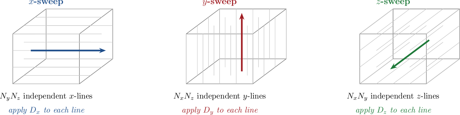
Production Cartesian solvers do not build that object. They exploit one identity, which a few pages of Kronecker algebra will make exact. With \(D_{xx}\), \(D_{yy}\), and \(D_{zz}\) the three one-dimensional second-derivative matrices (each of size \(200\), tridiagonal, a few kilobytes total), \[\Delta_h \;=\; I_z \otimes I_y \otimes D_{xx} \;+\; I_z \otimes D_{yy} \otimes I_x \;+\; D_{zz} \otimes I_y \otimes I_x.\] The \(8{,}000{,}000\times 8{,}000{,}000\) matrix on the left is the sum of three Kronecker products of the three small matrices on the right. We never build the object on the left. Applying \(\Delta_h\) to a field is three sweeps along the three families of grid lines, each sweep a batch of \(200\)-entry tridiagonal matvecs. A factored implicit method, such as ADI, replaces the coupled solve by the corresponding sequence of one-dimensional banded solves; a separable Poisson or Helmholtz solve uses the same directional structure through fast diagonalization. The algorithm lives inside the one-dimensional pieces. This is the picture behind every serious Cartesian solver, and the one 1 draws for the eye.
The idea is old in the best possible way. It has lived in direct-numerical-simulation solvers [1], [2], in FFT Poisson packages [3], and in spectral-element infrastructure for incompressible flow and acoustics [4] for decades. It is also the design logic behind pencil-decomposition libraries such as 2DECOMP&FFT [5], [6]. What has been missing is a single place where the argument is written down cleanly, once, for every discretization the reader is likely to care about, where the scope of the reduction is stated honestly, and where the production tricks that turn the argument into running floating-point code are ushered into the open.
The bookkeeping that makes the picture exact is the Kronecker product, which Van Loan memorably called “ubiquitous” [7] and which Strang uses as the running thread of computational linear algebra [8]. Two identities do most of the work: the mixed-product rule \((A \otimes B)(C \otimes D) = AC \otimes BD\), and the inverse rule \((A \otimes B)^{-1} = A^{-1} \otimes B^{-1}\). The first composes directional operators without ever forming their product. The second explains why a tensor-product mass matrix or compact line factor can be inverted by independent one-dimensional solves. Every subsequent section of this paper is a variation on those two identities plus the column-major vectorization rule.
The counting that makes the picture fast is even simpler. A one-dimensional banded matrix-vector product with bandwidth \(w_x\) costs \(\mathcal{O}(w_xN_x)\). A three-dimensional \(x\)-sweep is \(N_yN_z\) such products, hence \(\mathcal{O}(w_xN_xN_yN_z)=\mathcal{O}(w_xN)\). For fixed stencil width or fixed polynomial degree this is simply \(\mathcal{O}(N)\). Banded line solves have the same linear count, up to bandwidth constants, and fast transforms add their usual logarithmic factor. The full operator is large only if it is assembled; the line kernels are never large.
| Task | Tensor-product form | How it runs |
|---|---|---|
| Derivative sweep | \(I_z\kron I_y\kron D_x\) and relabelings | independent banded line applies, \(\bigO(\Nall)\) for fixed bandwidth |
| Compact derivative | \((I_z\kron I_y\kron A_x)v=(I_z\kron I_y\kron R_x)u\) | banded right-hand side plus banded line solve |
| Tensor-product mass inverse | \((M_z\kron M_y\kron M_x)^{-1}\) | three families of 1D mass solves |
| ADI substep | \(I-r(I_z\kron I_y\kron D_{xx})\) | one directional batch of line solves |
| Fast Poisson solve | diagonalized Kronecker sum | transforms by direction, scalar division, inverse transforms |
That combination, a Kronecker factorization for the algebra and a linewise count for the arithmetic, runs the whole paper. 2 makes both visible on a \(4 \times 3\) grid small enough to hold on one page, and recasts the 2D Poisson equation as a Sylvester matrix equation that makes the line action plain. 3 collects the two identities and fixes notation. [sec:1d-ops,sec:3d-ops] build the operator family from the one dimensional pieces: uniform and stretched grids, derivatives of all orders, mixed derivatives, the Laplacian. 6 handles compact Padé schemes and their implicit line structure [9], [10]. 7 extends the algebra to tensor-product Galerkin, B-spline, isogeometric, and collocation methods [11]–[15]. 8 folds in implicit time stepping through the classical Peaceman–Rachford and Douglas–Gunn ADI splittings [16]–[18]. 9 gives the direct-solver route by the Lynch–Rice–Thomas fast-diagonalization construction [19], [20]. 10 marks the boundary of what the framework can reach. 11 sets out the three implementation tricks that turn the algebra into efficient, hardware-conscious kernels on real machines. 12 measures the gap between assembling the three-dimensional matrix and never forming it on a model 3D Poisson solve. 13 is the implementation recipe in one page. The appendix collects the short derivations and the \(\operatorname{vec}{}\) identity that translate Kronecker formulas into explicit loops.
2 A two-dimensional motivating example↩︎
Small cases reveal the pattern. Let us take a 2D grid with \(N_x = 4\) points in \(x\) and \(N_y = 3\) points in \(y\) (boundary details ignored for clarity). The grid has \(4 \times 3 = 12\) points total, which is small enough to write every matrix on one page.
In 1D, the second-order central-difference first derivative on 4 points with spacing \(h\) is the tridiagonal matrix \[\label{eq:Dx-small} D_{x}= \frac{1}{2h} \begin{bmatrix} 0 & 1 & 0 & 0 \\ -1 & 0 & 1 & 0 \\ 0 & -1 & 0 & 1 \\ 0 & 0 & -1 & 0 \end{bmatrix} \in \mathbb{R}^{4 \times 4}.\tag{1}\] (One-sided stencils at the first and last rows would close the boundaries in a real code. The specific closure does not affect anything that follows.)
On the 2D grid, the objective is to compute \(\partial u / \partial x\) at all 12 points. Because the grid is Cartesian, the \(x\)-stencil at point \((i,j)\) depends only on the \(x\)-neighbors \((i-1,j)\) and \((i+1,j)\), at the same \(y\)-index \(j\). For each \(j\), \(D_{x}\) is therefore applied to the four values along the corresponding \(x\)-line:
| Line \(j=1\): | \(D_{x}\begin{bmatrix} u_{1,1} \\ u_{2,1} \\ u_{3,1} \\ u_{4,1} \end{bmatrix}\) |
| Line \(j=2\): | \(D_{x}\begin{bmatrix} u_{1,2} \\ u_{2,2} \\ u_{3,2} \\ u_{4,2} \end{bmatrix}\) |
| Line \(j=3\): | \(D_{x}\begin{bmatrix} u_{1,3} \\ u_{2,3} \\ u_{3,3} \\ u_{4,3} \end{bmatrix}\) |
The operation therefore consists of three independent applications of the same \(4 \times 4\) matrix. No two-dimensional matrix is formed.
2.1 Three dimensions is only a relabeling↩︎
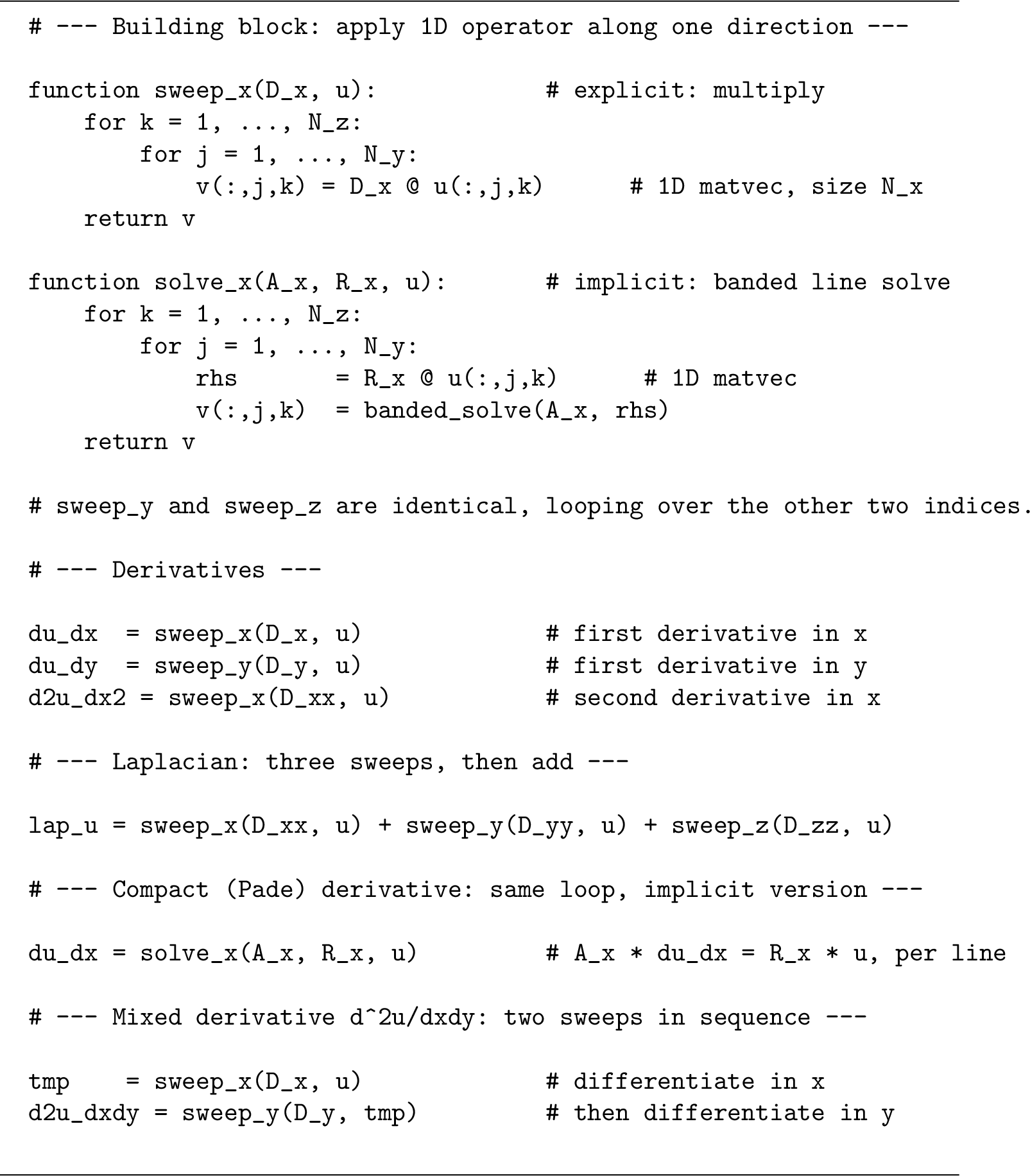
Moving the same argument to 3D changes nothing conceptual. The \(x\)-line, the \(y\)-line, and the \(z\)-line each play the role that the single \(x\)-line played above; each of them is swept by its own tridiagonal; each sweep is then stitched into the full field. 2 is a one-page template for the whole family. Every section that follows
instantiates these two building blocks, sweep and solve, with a different discretization.
If this action is written as a single matrix acting on all 12 unknowns at once (stacking the lines so that \(x\) varies fastest), the matrix would be the \(12 \times 12\) block-diagonal matrix \[\label{eq:block-diag} \begin{bmatrix} D_{x}& & \\ & D_{x}& \\ & & D_{x} \end{bmatrix} = I_3 \otimes D_{x},\tag{2}\] where \(I_3\) is the \(3 \times 3\) identity (one row per \(y\)-line) and \(\otimes\) denotes the Kronecker product. The notation “\(I_3 \otimes D_{x}\)” is a compact representation of “apply \(D_{x}\) to each line independently.” This linewise action is the core of the framework.
2.1.0.1 Poisson is a Sylvester equation in disguise.
There is a second picture of the same algebra, and it is the one mathematicians will recognize first. Arrange the unknowns into a rectangular array \(U \in \mathbb{R}^{N_x \times N_y}\), one column per \(y\)-line, and do not vectorize at all. The Laplacian acts by columns and by rows, \[\label{eq:sylvester-view} \Delta_h\, U \;=\; D_{xx}\, U \;+\; U\, D_{yy}^T,\tag{3}\] because \(D_{xx}\) differentiates down the columns and \(D_{yy}^T\) differentiates across the rows. The 2D Poisson problem \(-\Delta_hu = f\) is therefore the classical Sylvester matrix equation \[\label{eq:sylvester} -D_{xx}\, U - U\, D_{yy}^T \;=\; F,\tag{4}\] and the storage collapses to two small matrices and a rectangular grid of data: nothing of size \(N\times N\) appears anywhere. The equivalent long-vector form \(-(I_{y}\otimes D_{xx}+ D_{yy}\otimes I_{x})\,\operatorname{vec}(U) = \operatorname{vec}(F)\) says the same thing (14.3); the rectangular picture simply makes the directional action visible. Diagonalizing \(D_{xx}\) and \(D_{yy}\) in their own eigenbases uncouples the whole equation pointwise; that is the fast-diagonalization route of 9 [19]. The picture generalizes to three dimensions without change: the 3D Poisson problem is a three-term matrix equation on a tensor, with \(D_{xx}\), \(D_{yy}\), and \(D_{zz}\) acting each along its own coordinate axis.
3 Kronecker-product identities used throughout↩︎
The Kronecker product \(A \otimes B\) of an \(m \times n\) matrix \(A\) and a \(p \times q\) matrix \(B\) is the \(mp \times nq\) block matrix formed by replacing each entry \(a_{ij}\) of \(A\) with the block \(a_{ij}\,B\): \[\label{eq:kron-def} A \otimes B = \begin{bmatrix} a_{11} B & a_{12} B & \cdots & a_{1n} B \\ a_{21} B & a_{22} B & \cdots & a_{2n} B \\ \vdots & \vdots & \ddots & \vdots \\ a_{m1} B & a_{m2} B & \cdots & a_{mn} B \end{bmatrix}.\tag{5}\] Equation 2 shows that \(I_3 \otimes D_{x}\) produces the same block-diagonal matrix: the identity has ones on its diagonal, so each diagonal block is \(1 \cdot D_{x}= D_{x}\), and the off-diagonal blocks are \(0 \cdot D_{x}= 0\).
Only two standard identities are required for the developments that follow.
3.0.0.1 Property 1: the mixed-product rule.
If the matrix products \(AC\) and \(BD\) are defined, then \[\label{eq:mixed-product} (A \otimes B)(C \otimes D) = (AC) \otimes(BD).\tag{6}\] That is, the corresponding factors multiply independently. This identity underlies the composition of directional operators.
3.0.0.2 Property 2: the inverse rule.
If \(A\) and \(B\) are both invertible, then \[\label{eq:kron-inv} (A \otimes B)^{-1} = A^{-1} \otimes B^{-1}.\tag{7}\] This follows from the mixed-product rule: \((A \otimes B)(A^{-1} \otimes B^{-1}) = (AA^{-1}) \otimes(BB^{-1}) = I \otimes I = I\).
These identities, together with the vectorization convention below, are enough for every construction in the paper. They belong to a much larger body of Kronecker-product algebra treated systematically by [7], [21] and, in the higher-order-tensor setting, by [22]. Appendix 14 records the short derivations and the \(\operatorname{vec}{}\) identity that converts the abstract Kronecker formulas into explicit line sweeps.
3.0.0.3 Vectorization convention.
One bookkeeping detail concerns how a 2D array \(U(i,j)\) is flattened into a vector \(\boldsymbol{u}\): columns are stacked so that the \(x\)-index varies fastest. For a \(4 \times 3\) grid: \[\boldsymbol{u} = \bigl[ u_{1,1},\; u_{2,1},\; u_{3,1},\; u_{4,1},\; u_{1,2},\; u_{2,2},\; \ldots,\; u_{4,3} \bigr]^T.\] In 3D, the ordering is \(x\) fastest, then \(y\), then \(z\). This column-major ordering is what makes the Kronecker product formulas come out with the rightmost factor acting on \(x\), the middle factor on \(y\), and the leftmost on \(z\).
4 One-dimensional finite-difference operators↩︎
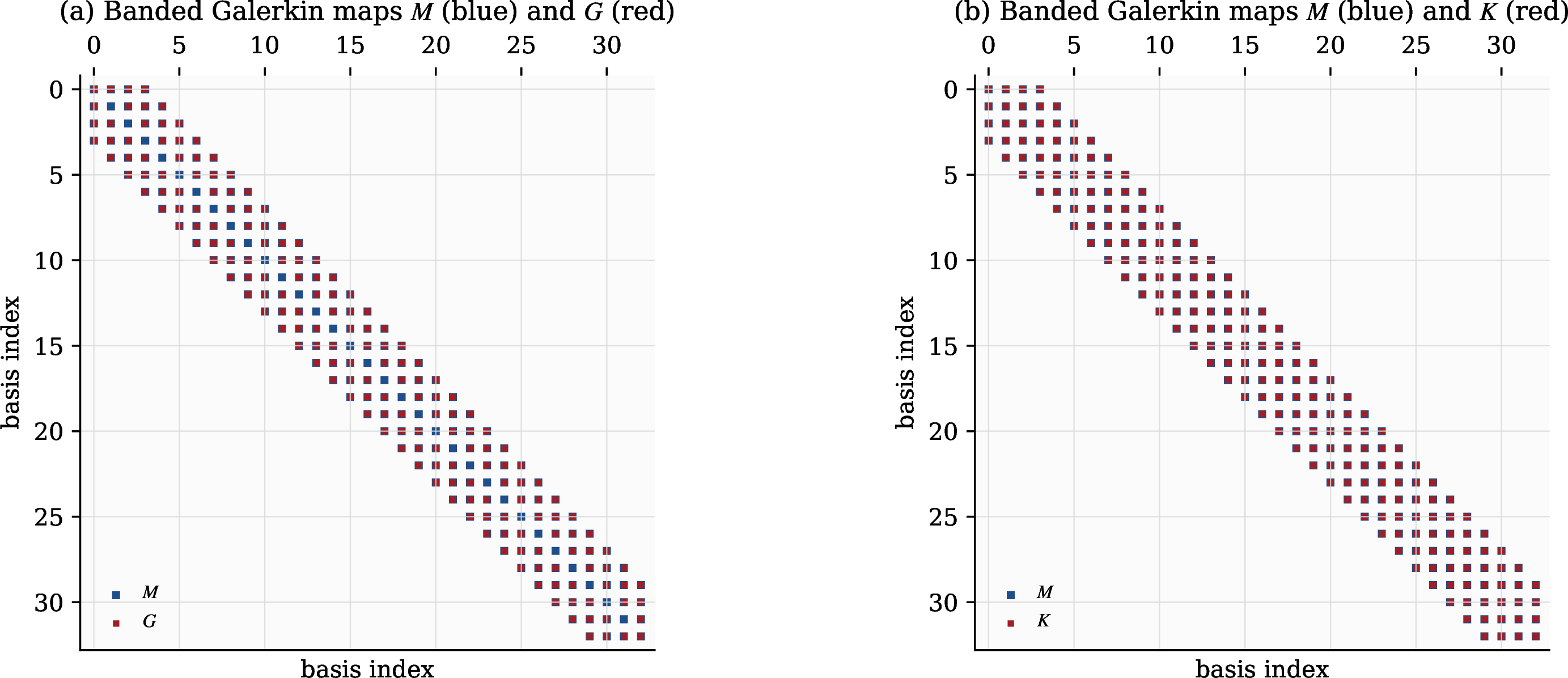
This section collects the 1D building blocks. On a non-uniform grid, the operator remains banded and only the entries change. 3 emphasizes this structure before the formulas are introduced. The first- and second-derivative maps occupy thin bands around the diagonal. Consequently, a full 3D sweep remains linear in \(N\): every output value depends on only a fixed number of nearby inputs, with no long-range fill-in and no dense intermediate state.

4.1 Uniform grids↩︎
On a uniform grid \(x_i = x_0 + i\,h\), the standard central-difference approximations are: \[\begin{align} \text{First derivative:} \quad u'(x_i) &\approx \frac{u_{i+1} - u_{i-1}}{2h}, \tag{8} \\[4pt] \text{Second derivative:} \quad u''(x_i) &\approx \frac{u_{i-1} - 2u_i + u_{i+1}}{h^2}. \tag{9} \end{align}\] Collecting these for all grid points gives the tridiagonal matrices \(D_{x}\) and \(D_{xx}\). Applying either to a vector of length \(N_x\) costs \(\mathcal{O}(N_x)\) operations. Higher-order stencils (fourth-order, sixth-order) widen the bandwidth but do not change the structure [23]. In three dimensions, the operator is obtained by repeating the same one-dimensional banded apply on many parallel lines.
4.1.0.1 Boundary closures.
Equations 8 –9 apply at interior points. The endpoint rows of \(D_{x}\) and \(D_{xx}\) require boundary closures. A standard second-order first-derivative closure uses \(u'(x_1) \approx (-3 u_1 + 4 u_2 - u_3)/(2h)\) and the reflected formula at \(x_{N_x}\); a second-order second-derivative closure may use \((2u_1-5u_2+4u_3-u_4)/h^2\) at the left endpoint and the reflected row at the right endpoint. Compact, Galerkin, and B-spline discretizations carry their own closure families ([9]; [11]). The choice of closure modifies only a small number of boundary rows in the 1D operator, leaves the interior banded structure intact, and inherits into the 3D apply with no change to the Kronecker factorization.
4.1.0.2 The line solver: Thomas algorithm.
Every implicit line operation in this paper invokes a banded triangular solve, and for tridiagonal systems the workhorse is the Thomas algorithm [24]. Given \(A_{x}\boldsymbol{x} = \boldsymbol{d}\) with \(A_{x}\) tridiagonal of subdiagonal \(a_i\), diagonal \(b_i\), and superdiagonal \(c_i\), the forward sweep eliminates the subdiagonal. With \(\tilde{c}_1=c_1/b_1\) and \(\tilde{d}_1=d_1/b_1\), the interior rows \(i=2,\ldots,N_\xi-1\) use \[\label{eq:thomas-fwd} m_i = b_i-a_i\tilde{c}_{i-1},\quad \tilde{c}_i = \frac{c_i}{m_i},\quad \tilde{d}_i = \frac{d_i-a_i\tilde{d}_{i-1}}{m_i},\tag{10}\] and the final row closes the sweep with \(m_{N_\xi} = b_{N_\xi}-a_{N_\xi}\tilde{c}_{N_\xi-1}\) and \(\tilde{d}_{N_\xi} = (d_{N_\xi}-a_{N_\xi}\tilde{d}_{N_\xi-1})/m_{N_\xi}\). These formulas assume the pivots \(m_i\) are nonzero. That is the usual case for the diagonally dominant elliptic line factors that motivate the discussion; otherwise one must use pivoting or a more general banded solver. The backward sweep recovers the solution: \[\label{eq:thomas-bwd} x_{N_\xi} = \tilde{d}_{N_\xi}, \qquad x_i = \tilde{d}_i - \tilde{c}_i\, x_{i+1}, \qquad i = N_\xi-1, \ldots, 1.\tag{11}\] The total cost is \(\mathcal{O}(N_\xi)\) operations (a small constant number of flops per row) and only \(\mathcal{O}(N_\xi)\) memory traffic per line. A banded solve with semibandwidth \(w\) replaces the two scalar updates above with \(\mathcal{O}(w^2)\) local elimination work per row for a general banded factorization, or \(\mathcal{O}(w)\) work when a fixed-band LU factor has already been computed. In either case, for fixed \(w\) the line solve is linear in \(N_\xi\). A 3D implicit sweep is \(N/N_\xi\) independent invocations of this two-pass kernel.
4.2 Non-uniform grids↩︎
Now let the spacing vary: \(h_i^{+} = x_{i+1} - x_i\) and \(h_i^{-} = x_i - x_{i-1}\). The three-point central formulas extend to \[\begin{align} u'(x_i) &\approx \frac{ -(h_i^{+})^2 \, u_{i-1} + \bigl[(h_i^{+})^2 - (h_i^{-})^2\bigr] u_i + (h_i^{-})^2 \, u_{i+1} }{ h_i^{+}\, h_i^{-}\, (h_i^{+} + h_i^{-}) }, \tag{12} \\[4pt] u''(x_i) &\approx \frac{2}{h_i^{+} + h_i^{-}} \left( \frac{u_{i+1} - u_i}{h_i^{+}} - \frac{u_i - u_{i-1}}{h_i^{-}} \right). \tag{13} \end{align}\] On a uniform grid, 12 reduces to \((u_{i+1} - u_{i-1})/(2h)\) and 13 reduces to \((u_{i-1} - 2 u_i + u_{i+1})/h^2\). A Taylor expansion gives two useful cautions. The first-derivative formula 12 is exact for quadratics and has a second-order local truncation error when the adjacent spacings are comparable. The three-point second-derivative formula 13 is also exact for quadratics, but its leading cubic error is proportional to \(h_i^{+}-h_i^{-}\). Thus it is second order on smoothly mapped grids where \(h_i^{+}-h_i^{-}=\mathcal{O}(h^2)\), but only first order on a strongly irregular grid where that difference is \(\mathcal{O}(h)\). If one needs second-order accuracy on arbitrary non-uniform point sets, a wider stencil generated by Fornberg’s algorithm [23] or a smooth coordinate transform is the safer choice. In every case the stencil weights vary from point to point, but the operator remains banded.
For the purposes of this paper, the essential point is that a non-uniform Cartesian grid is still a tensor product of 1D grids, so the Kronecker product structure is unchanged. The one-dimensional matrices acquire non-constant diagonals, but the geometry may stretch, cluster, or bias the points without changing the cost model: banded 1D operators still give linear-time sweeps in the total number of grid values.
5 From 1D to 3D: every operator, one identity at a time↩︎
The same Kronecker machinery produces the whole operator family. Throughout this section, \(I_{x}\), \(I_{y}\), \(I_{z}\) are identity matrices of sizes \(N_x\), \(N_y\), \(N_z\), and \(\boldsymbol{u} \in \mathbb{R}^{N}\) is the flattened field with \(x\) varying fastest. The rule for reading any triple Kronecker product is the same in every case: the rightmost factor acts on the fastest (\(x\)) index, the middle factor on \(y\), the leftmost on \(z\).
5.1 First derivatives↩︎
The central-difference approximation to \(\partial u/\partial x\) at the interior point \((i,j,k)\), \[\label{eq:3d-dx-pointwise} \left(\frac{\partial u}{\partial x}\right)_{ijk} \approx \frac{u_{i+1,j,k} - u_{i-1,j,k}}{2h_x},\tag{14}\] touches only the two \(x\)-neighbors at the same \((j,k)\). The directional Kronecker placement is therefore dictated by 14 itself: \[\label{eq:3d-Dx} \boxed{ \frac{\partial \boldsymbol{u}}{\partial x} = (I_{z}\otimes I_{y}\otimes D_{x})\,\boldsymbol{u}. }\tag{15}\] Reading this equation as an algorithm: for each pair \((j,k)\), apply the small banded \(D_{x}\) to the \(x\)-line \(u(:,j,k)\). The outer identity factors \(I_{y}\) and \(I_{z}\) say the \(y\) and \(z\) indices are passengers during an \(x\)-sweep; they come along for the ride. The \(y\)- and \(z\)-derivatives are obtained by sliding the derivative block into the appropriate slot, \[\label{eq:3d-Dy-Dz} \frac{\partial \boldsymbol{u}}{\partial y} = (I_{z}\otimes D_{y}\otimes I_{x})\,\boldsymbol{u}, \qquad \frac{\partial \boldsymbol{u}}{\partial z} = (D_{z}\otimes I_{y}\otimes I_{x})\,\boldsymbol{u},\tag{16}\] and the rest of the pattern follows. A full sweep in any direction touches each of the \(N\) grid values a fixed number of times, so the cost is the optimal \(\mathcal{O}(N)\).
5.2 Second derivatives↩︎
The second derivative needs no new ideas. Swap \(D_{x}\) for the tridiagonal \(D_{xx}\) and do it again: \[\label{eq:3d-Dxx} \frac{\partial^2 \boldsymbol{u}}{\partial x^2} = (I_{z}\otimes I_{y}\otimes D_{xx})\,\boldsymbol{u}, \quad \frac{\partial^2 \boldsymbol{u}}{\partial y^2} = (I_{z}\otimes D_{yy}\otimes I_{x})\,\boldsymbol{u}, \quad \frac{\partial^2 \boldsymbol{u}}{\partial z^2} = (D_{zz}\otimes I_{y}\otimes I_{x})\,\boldsymbol{u}.\tag{17}\] The kernel is different. The algorithm is the same.
5.3 Mixed derivatives↩︎
The mixed derivative \(\partial^2 u / \partial x\,\partial y\) is two sweeps in a row, one per direction. The mixed-product rule (14.1) collapses the composition into a single Kronecker product: \[\label{eq:3d-Dxy} \frac{\partial^2 \boldsymbol{u}}{\partial x\,\partial y} = \underbrace{(I_{z}\otimes D_{y}\otimes I_{x})}_{\text{then } y} \underbrace{(I_{z}\otimes I_{y}\otimes D_{x})}_{\text{first } x}\,\boldsymbol{u} \;=\; (I_{z}\otimes D_{y}\otimes D_{x})\,\boldsymbol{u}.\tag{18}\] The right-hand side is cosmetic. The code still executes two sweeps, an intermediate field between them, and never builds the dense product \(D_{y}\otimes D_{x}\).
5.4 The Laplacian↩︎
The seven-point discrete Laplacian at the interior point \((i,j,k)\), \[\label{eq:laplacian-pointwise} (\Delta_h\,u)_{ijk} \;=\; \frac{u_{i-1,j,k} {-} 2u_{ijk} {+} u_{i+1,j,k}}{h_x^2} + \frac{u_{i,j-1,k} {-} 2u_{ijk} {+} u_{i,j+1,k}}{h_y^2} + \frac{u_{i,j,k-1} {-} 2u_{ijk} {+} u_{i,j,k+1}}{h_z^2},\tag{19}\] is the sum of three single-direction second derivatives. Each term looks at only one coordinate. That is why the Laplacian falls immediately into three additive sweeps, \[\label{eq:3d-laplacian} \Delta_h\,\boldsymbol{u} \;=\; (I_{z}\otimes I_{y}\otimes D_{xx})\,\boldsymbol{u} \,+\, (I_{z}\otimes D_{yy}\otimes I_{x})\,\boldsymbol{u} \,+\, (D_{zz}\otimes I_{y}\otimes I_{x})\,\boldsymbol{u},\tag{20}\] which is exactly the identity that powered the introduction. The three results are computed line by line and added at the end.
5.5 Memory layout and sweep direction↩︎
An \(x\)-sweep is effortless because consecutive \(x\)-points sit next to each other in memory. A \(y\)-sweep strides across \(N_x\) elements to reach the next grid point in its line, and a \(z\)-sweep strides across \(N_x N_y\). Two remedies exist: walk the stride with gather and scatter, or transpose the active direction into the fast axis before sweeping and transpose back afterward. On modern caches and accelerators the transpose almost always wins. That is the serial picture. Its distributed counterpart is the pencil decomposition (11.3), in which the transpose becomes a collective MPI operation between global orientations of the field. In both cases the 1D kernel is unchanged; only the data motion around it moves.
6 Compact (Padé) schemes↩︎
Compact schemes trade a wider explicit stencil for a narrower implicit relation: instead of writing the derivative as a long sum of neighbor values, they couple a few nearby derivative values together [9], [10]. The reward is spectral-like accuracy with a three-point stencil. The price, or what looks like a price on paper, is that one can no longer write \(\boldsymbol{u}' = D_{x}\, \boldsymbol{u}\) with a banded \(D_{x}\). Instead, one writes \[A_{x}\, \boldsymbol{u}' \;=\; R_{x}\, \boldsymbol{u},\] with \(A_{x}\) and \(R_{x}\) both banded. The algebraically equivalent statement \(\boldsymbol{u}' = A_{x}^{-1}R_{x}\, \boldsymbol{u}\) conceals a pitfall: \(A_{x}^{-1}R_{x}\) is generically dense. 4 shows why the factorized form is the only one that should ever touch memory. Both matrices are tridiagonal. Keep them that way: apply \(R_{x}\) (banded matvec, \(\mathcal{O}(N_x)\)), then solve with \(A_{x}\) (Thomas algorithm [24], \(\mathcal{O}(N_x)\)). Total work per line: \(\mathcal{O}(N_x)\). Total work per 3D sweep: \(\mathcal{O}(N)\). The compact scheme has the same asymptotic cost as central differences, with a larger but controlled constant and typically much better resolution per grid point.

6.0.0.1 Example: fourth-order Padé first derivative.
The classical fourth-order Padé first derivative in 1D reads [9] \[\label{eq:pade-example} \tfrac{1}{4}\,u'_{i-1} + u'_i + \tfrac{1}{4}\,u'_{i+1} = \tfrac{3}{2}\,\frac{u_{i+1} - u_{i-1}}{2h}.\tag{21}\] The two coefficients \(\alpha = 1/4\) and \(a = 3/2\) are determined by matching the Taylor expansion through fourth order; the same construction yields the sixth-order tridiagonal scheme with \(\alpha = 1/3\), \(a = 14/9\), and \(b = 1/9\) on a wider right-hand-side stencil [9]. The left-hand side couples three derivative values, hence the term “compact,” while the right-hand side uses the standard centered stencil with a modified coefficient. In matrix form this is \(A_{x}\,\boldsymbol{u}' = R_{x}\,\boldsymbol{u}\), where \(A_{x}\) is tridiagonal with \(1\) on the main diagonal and \(1/4\) on the sub- and super-diagonals, and \(R_{x}\) encodes the right-hand side stencil. The equivalent expression \(\boldsymbol{u}' = A_{x}^{-1}R_{x}\,\boldsymbol{u}\) is algebraically correct, but the implementation proceeds by applying \(R_{x}\) and solving with \(A_{x}\), rather than by forming \(A_{x}^{-1}\).
6.0.0.2 Three-dimensional form.
In three dimensions, the compact scheme for \(\partial u/\partial x\) at each point \((i,j,k)\) reads \[\label{eq:compact-3d-pointwise} \tfrac{1}{4}\,u'_{i-1,j,k} + u'_{ijk} + \tfrac{1}{4}\,u'_{i+1,j,k} = \tfrac{3}{2}\,\frac{u_{i+1,j,k} - u_{i-1,j,k}}{2h_x}.\tag{22}\] Written for all \(N_x N_y N_z\) points simultaneously, this is the system \(\mathcal{A}\,\boldsymbol{u}' = \mathcal{R}\,\boldsymbol{u}\), where \(\mathcal{A}\) and \(\mathcal{R}\) are \(N\times N\) matrices. Solving this as a monolithic system would be prohibitively expensive. But because the coupling on both sides is only along \(x\) (the indices \(j\) and \(k\) are the same on both sides of the equation), the system decomposes.
6.0.0.3 Kronecker form of compact schemes.
The 3D compact first derivative in \(x\) factors as \[\label{eq:3d-compact-Dx} (I_{z}\otimes I_{y}\otimes A_{x})\;\boldsymbol{v} = (I_{z}\otimes I_{y}\otimes R_{x})\;\boldsymbol{u},\tag{23}\] where \(\boldsymbol{v}\) is the vector of derivative values. Because \(A_{x}\) appears inside the same Kronecker product structure, this system decomposes into \(N_y \cdot N_z\) independent tridiagonal solves of size \(N_x\), one per \(x\)-line. Each line costs \(\mathcal{O}(N_x)\), so the full sweep costs \(\mathcal{O}(N)\). The higher dimension does not change the kernel. It only increases the number of identical lines to be processed. Appendix 14.5 writes this decomposition out explicitly in \(\operatorname{vec}{}\) form.
For a fixed \((j,k)\), the line operation is:
Compute the right-hand side: \(\boldsymbol{b} = R_{x}\,u(:,j,k)\) (banded matrix-vector product, \(\mathcal{O}(N_x)\)).
Solve the tridiagonal system: \(A_{x}\,v(:,j,k) = \boldsymbol{b}\) via the Thomas algorithm (\(\mathcal{O}(N_x)\)).
Repeat for all \((j,k)\) pairs. The \(y\)- and \(z\)-compact derivatives are the same, with the appropriate direction: \[(I_{z}\otimes A_{y}\otimes I_{x})\;\boldsymbol{v} = (I_{z}\otimes R_{y}\otimes I_{x})\;\boldsymbol{u}, \qquad (A_{z}\otimes I_{y}\otimes I_{x})\;\boldsymbol{v} = (R_{z}\otimes I_{y}\otimes I_{x})\;\boldsymbol{u}.\] Compact second derivatives (\(A_{xx}\), \(R_{xx}\), etc.) work identically. The same factorized viewpoint applies. The effective map \(A_{xx}^{-1}R_{xx}\) may be dense when written explicitly, but the banded apply remains linear-time because that dense product is never formed.
6.0.0.4 Non-uniform grids.
Compact schemes can be derived on non-uniform grids by matching Taylor expansions with the local spacing. The matrices \(A_{x}\) and \(R_{x}\) get point-dependent entries, but they remain tridiagonal, and the Kronecker structure is unchanged. The same factorized line solve survives on stretched grids without any asymptotic penalty.
7 Galerkin and B-spline methods↩︎
Finite differences are not special. Every Cartesian discretization that uses a tensor-product basis factors the same way: a finite-element method, a spectral-element method, a Fourier or Chebyshev expansion, a B-spline collocation, an isogeometric analysis. The ingredients have different names, but the Kronecker machinery is identical. This section tracks the factorization through the weak form.
7.1 Galerkin on a tensor-product domain↩︎
On the box \(\Omega = [a,b] \times [c,d] \times [e,f]\), the Galerkin recipe for \(-\nabla^2 u = g\) expands the solution in basis functions \(\{\Phi_n\}\), tests against the same family, and integrates by parts to produce \(K \hat{\boldsymbol{u}} = \boldsymbol{g}\) with \[\label{eq:3d-mass-full} M_{mn} = \int_\Omega \Phi_m \Phi_n \, d\boldsymbol{x}, \qquad K_{mn} = \int_\Omega \nabla\Phi_m \cdot \nabla\Phi_n \, d\boldsymbol{x}.\tag{24}\] Written at face value, \(M\) and \(K\) are \(N\times N\). Written with eyes open, they are not. The 1D Galerkin building blocks are banded (5), and the 3D operators inherit that locality through a Kronecker factorization that is about to fall out of the geometry of the basis.
7.1.0.1 The 3D operators factor.
On a tensor-product domain with a tensor-product basis, every 3D basis function splits as \[\label{eq:galerkin-basis} \Phi_{ijk}(x,y,z) = \phi^x_i(x)\,\phi^y_j(y)\,\phi^z_k(z),\tag{25}\] and \(d\boldsymbol{x}\) factors with it. The 3D mass integral is therefore the product of three 1D integrals, \[\label{eq:mass-factor} M_{(ijk),(pqr)} = \underbrace{\int \phi^x_i\,\phi^x_p\,dx}_{(M_x)_{ip}} \;\underbrace{\int \phi^y_j\,\phi^y_q\,dy}_{(M_y)_{jq}} \;\underbrace{\int \phi^z_k\,\phi^z_r\,dz}_{(M_z)_{kr}}.\tag{26}\] This is exactly the Kronecker product: \[\label{eq:3d-mass} \boxed{ M = M_z \otimes M_y \otimes M_x }\tag{27}\]
For the stiffness matrix, the gradient introduces a derivative in one direction at a time. Taking the \(x\)-contribution as an example: \[\int_\Omega \frac{\partial\Phi_{ijk}}{\partial x} \frac{\partial\Phi_{pqr}}{\partial x}\,d\boldsymbol{x} = \underbrace{\int \phi'^x_i\,\phi'^x_p\,dx}_{(K_x)_{ip}} \;\underbrace{\int \phi^y_j\,\phi^y_q\,dy}_{(M_y)_{jq}} \;\underbrace{\int \phi^z_k\,\phi^z_r\,dz}_{(M_z)_{kr}}.\] Summing over all three gradient components gives the full stiffness matrix: \[\label{eq:3d-stiffness} K = M_z \otimes M_y \otimes K_x + M_z \otimes K_y \otimes M_x + K_z \otimes M_y \otimes M_x.\tag{28}\] The Galerkin semi-discrete system for the time-dependent problem \(\partial u/\partial t = \nabla^2 u\) is \(M\,\dot{\boldsymbol{u}} = -K\,\boldsymbol{u} + \boldsymbol{f}\), and it inherits full Kronecker structure.
7.1.0.2 Mass inversion and stiffness apply.
An explicit step needs \(M^{-1}\) at every stage. The inverse rule 7 gives it without a fight: \[M^{-1} = M_z^{-1} \otimes M_y^{-1} \otimes M_x^{-1},\] and applying \(M^{-1}\) is three passes of 1D banded solves along the three line families. Each \(M_\xi\) is tridiagonal for linear elements, pentadiagonal for quadratics, and banded with bandwidth \(2p+1\) for splines of degree \(p\), so every pass is \(\mathcal{O}(N_\xi)\) per line and \(\mathcal{O}(N)\) across the grid. The stiffness apply \(K\boldsymbol{u}\) is the same story played three times, once for each term in 28 ; never form the Kronecker product explicitly, apply each factor along its own direction and add.
7.1.0.3 Spectral methods are the same story.
With global polynomials (Chebyshev, Legendre) or Fourier modes, the 1D mass matrices become diagonal in an orthogonal basis and the stiffness matrices keep their Kronecker-sum shape. Spectral element methods restrict the same construction to each tensor-product element and reap the same line structure [4], [20]. None of the algebra changes; only the 1D pieces become polynomial rather than finite-difference.
7.2 B-spline and isogeometric discretizations↩︎
B-splines are the discretization the Kronecker picture was waiting for [11]. In 1D, a spline of degree \(p\) is a linear combination \(u(x) = \sum_i B^x_i(x)\,\alpha_i\) of compactly supported basis functions, and the coefficient vector \(\alpha\) is the object one stores. Evaluating the spline and its derivatives is a linear map: \[u(x) = B(x)\,\alpha, \qquad u_x(x) = B'(x)\,\alpha, \qquad u_{xx}(x) = B''(x)\,\alpha,\] the spline analog of a 1D differentiation matrix. The evaluation maps \(B\), \(B'\), and \(B''\) have only \(\mathcal{O}(p)\) nonzeros per row: at any point, at most \(p+1\) B-splines are active. The Galerkin mass and stiffness matrices assembled from these maps have bandwidth \(\mathcal{O}(p)\), commonly written as \(2p+1\) for open knot vectors. The same banded structure appears in the boundary-consistent filtering construction used for high-fidelity turbulence [15], which again replaces a three-dimensional filter by repeated one-dimensional spline maps. The same tensor-product spline structure also governs the statistical problem: used as a regression basis rather than a discretization, it makes the optimal resolution solvable in closed form—its cost set by interaction order rather than ambient dimension—instead of found by search [25].
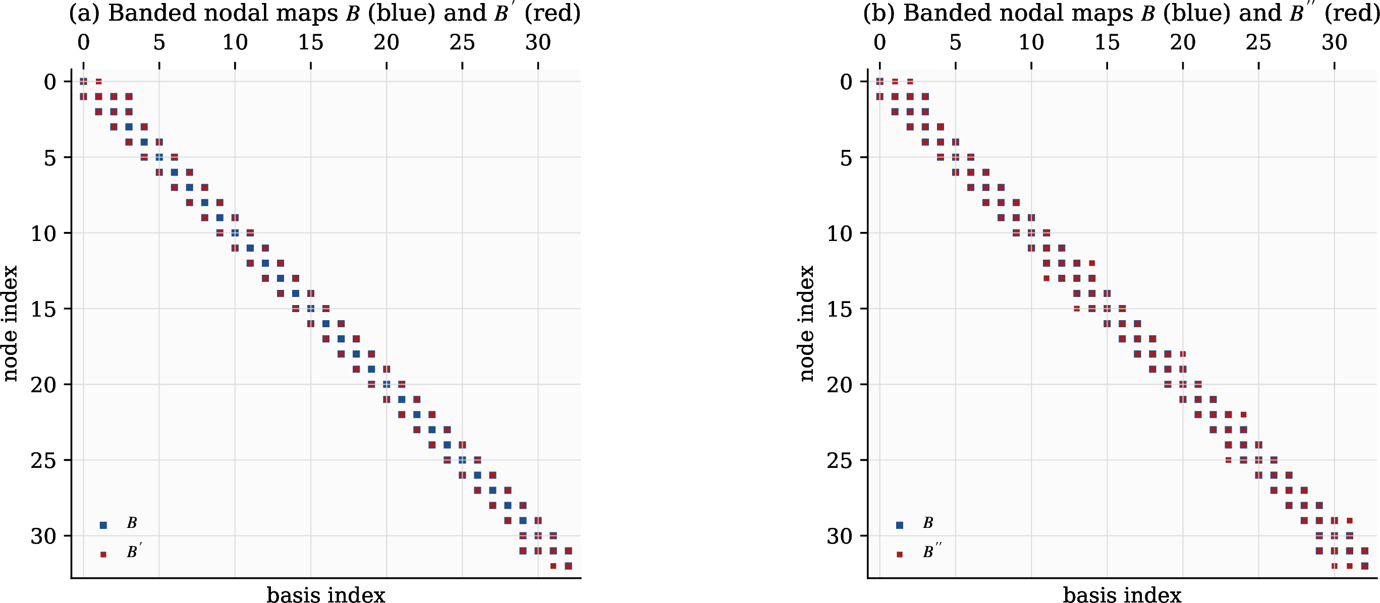
Choose evaluation or quadrature points \(\{x_q\}_{q=1}^{Q_x}\) and form the matrices \[(B_x)_{qi} = B^x_i(x_q), \qquad (B_x')_{qi} = \frac{dB^x_i}{dx}(x_q), \qquad (B_x'')_{qi} = \frac{d^2 B^x_i}{dx^2}(x_q).\] If \(u \in \mathbb{R}^{Q_x}\) denotes the vector of sampled spline values \(u_q = u(x_q)\), then \[u = B_x \alpha, \qquad u_x = B_x' \alpha, \qquad u_{xx} = B_x'' \alpha.\] For Galerkin assembly, let \(W_x = \operatorname{diag}(w_1,\ldots,w_{Q_x})\) be the diagonal matrix of quadrature weights. The 1D Galerkin matrices are then \[M_x = B_x^T W_x B_x, \qquad G_x = B_x^T W_x B_x', \qquad K_x = (B_x')^T W_x B_x'.\] Here \(M_x\) is the 1D mass matrix, \(G_x\) is the first-derivative coupling matrix, and \(K_x\) is the 1D stiffness matrix. The same construction gives \(M_y\), \(M_z\), \(G_y\), \(G_z\), \(K_y\), and \(K_z\). In three dimensions, \[u(x,y,z) = \sum_{i=1}^{N_x}\sum_{j=1}^{N_y}\sum_{k=1}^{N_z} \alpha_{ijk}\, B^x_i(x)\, B^y_j(y)\, B^z_k(z),\] and the assembled operators are still \[M = M_z \otimes M_y \otimes M_x, \qquad K = M_z \otimes M_y \otimes K_x + M_z \otimes K_y \otimes M_x + K_z \otimes M_y \otimes M_x.\] The 3D spline solve therefore has the same tensor-product structure as the finite-element case above. The only additional ingredient is the assembly of the 1D matrices. Because each spline overlaps only \(\mathcal{O}(p)\) neighbors, the 1D mass and stiffness matrices remain banded with bandwidth \(2p+1\), and every line operation remains \(\mathcal{O}(N_\xi)\). Consequently, the 3D Galerkin or isogeometric apply is linear in \(N\) because it is built entirely from these banded 1D blocks.
7.2.0.1 Isogeometric analysis.
In isogeometric analysis (IGA) [12], [13], the same B-spline (or NURBS) basis that represents the CAD geometry is reused as the solution basis. This gives exact CAD geometry on each tensor-product patch, while preserving the same operator algebra. On a box-shaped parameter domain, the primary unknown is usually the coefficient vector \(\alpha\), not sampled values \(u\). If one wants the values of the derivative at sample points, the apply is direct: \[u_x = B_x' \alpha.\] If instead one wants a derivative operator that maps spline coefficients to spline coefficients in the same basis, introduce coefficients \(\beta_x\) such that \(B(x)\,\beta_x\) is the \(L^2\) projection of \(u_x\) back into the spline space. The 1D projection equation is \[M_x \beta_x = G_x \alpha, \qquad\text{so}\qquad \beta_x = D_x^{\mathrm{IGA}} \alpha, \qquad D_x^{\mathrm{IGA}} = M_x^{-1} G_x.\] This is the IGA analog of applying a 1D derivative matrix along a line. But the factorized form is the computational one that matters: apply \(G_x\), then solve with \(M_x\). If one forms \(M_x^{-1}G_x\) explicitly, that product is generally dense. In 3D, the same operator factors as \[I_z \otimes I_y \otimes D_x^{\mathrm{IGA}},\] and similarly in \(y\) and \(z\). For diffusion and Poisson problems, the second-derivative action usually enters through the stiffness matrix \(K_x\) rather than an explicit pointwise \(D_{xx}\).
The computational consequence is therefore straightforward: IGA changes the basis and often improves accuracy per degree of freedom through higher continuity, but it does not alter the 3D apply. Once the 1D spline matrices are assembled, every matrix-vector product or implicit solve remains a batch of 1D line operations.
7.2.0.2 B-spline collocation.
An alternative to the Galerkin approach is B-spline collocation: instead of integrating against test functions, evaluate the PDE directly at a set of collocation points and require the B-spline expansion to satisfy the equation pointwise. A common choice is the Greville points [14], but the tensor algebra does not depend on the specific set of collocation sites. In 1D, evaluate the basis and its derivatives at the collocation points to obtain square matrices \(B_x\), \(B_x'\), and \(B_x''\). If \(u\) denotes the vector of spline values at those points, then \[u = B_x \alpha, \qquad u_x = B_x' \alpha, \qquad u_{xx} = B_x'' \alpha.\] Eliminating the coefficients gives the collocation differentiation matrices \[D_{x}= B_x' B_x^{-1}, \qquad D_{xx}= B_x'' B_x^{-1}.\] These are the spline-induced first- and second-derivative matrices on collocated values. They are useful for analysis, but they are not the best objects to form in code. The matrices \(B_x\), \(B_x'\), and \(B_x''\) in 6 are banded, whereas \(B_x^{-1}\) is generally dense. So the linear-time collocation apply should be read in factorized form: solve \(B_x \alpha = u\) on each line, then apply \(B_x'\) or \(B_x''\) to that recovered coefficient line. Appendix 14.5 writes the same coefficient-recovery step directly in tensor-product form. This banded solve plus banded matvec still costs \(\mathcal{O}(N_x)\) per line and therefore \(\mathcal{O}(N)\) over the full 3D grid. In periodic shift-invariant settings, these formed matrices can become circulant and enjoy useful symmetry properties, but they are still not generically banded once \(B_x^{-1}\) is formed.
In coefficient form, the 3D collocation Poisson operator can be written without ever introducing a dense value-space differentiation matrix: \[-\bigl( B_z \otimes B_y \otimes B_x'' + B_z \otimes B_y'' \otimes B_x + B_z'' \otimes B_y \otimes B_x \bigr)\,\alpha = \boldsymbol{g}.\] This representation is the cleanest implementation form because every factor on every line is banded.
For the Poisson equation \(-\nabla^2 u = g\), the full 3D collocation system on collocated values can also be written as \[-\bigl(I_{z}\otimes I_{y}\otimes D_{xx} + I_{z}\otimes D_{yy}\otimes I_{x} + D_{zz}\otimes I_{y}\otimes I_{x}\bigr)\,\boldsymbol{u} = \boldsymbol{g},\] where \(D_{xx}\), \(D_{yy}\), \(D_{zz}\) are the spline collocation second-derivative matrices in each direction. This is a Kronecker sum, identical in structure to the finite-difference Laplacian 20 , and it can be solved by the same fast diagonalization technique (9).
Collocation avoids numerical quadrature entirely, which simplifies setup. The computational message is the same as for compact schemes: use the factorized banded maps, not a preformed dense derivative matrix, and the per-line operations remain exactly
the same sweep and solve from the pseudocode (2).
8 Implicit time stepping via ADI↩︎
Stiffness forces an implicit treatment. For the heat equation on a fine grid, the explicit stability limit \(\Delta t\lesssim h^2/\nu\) is prohibitive, and implicit methods lift that ceiling by solving a system at each step. In three dimensions that system is \(N\times N\). Forming it is out of the question. The classical cure, invented in the 1950s for oil-reservoir simulation by [16] and generalized to three space variables by [17], [18], is the alternating-direction implicit (ADI) splitting: replace one coupled 3D solve by three 1D solves, one per direction, each of which is a batch of banded line solves.
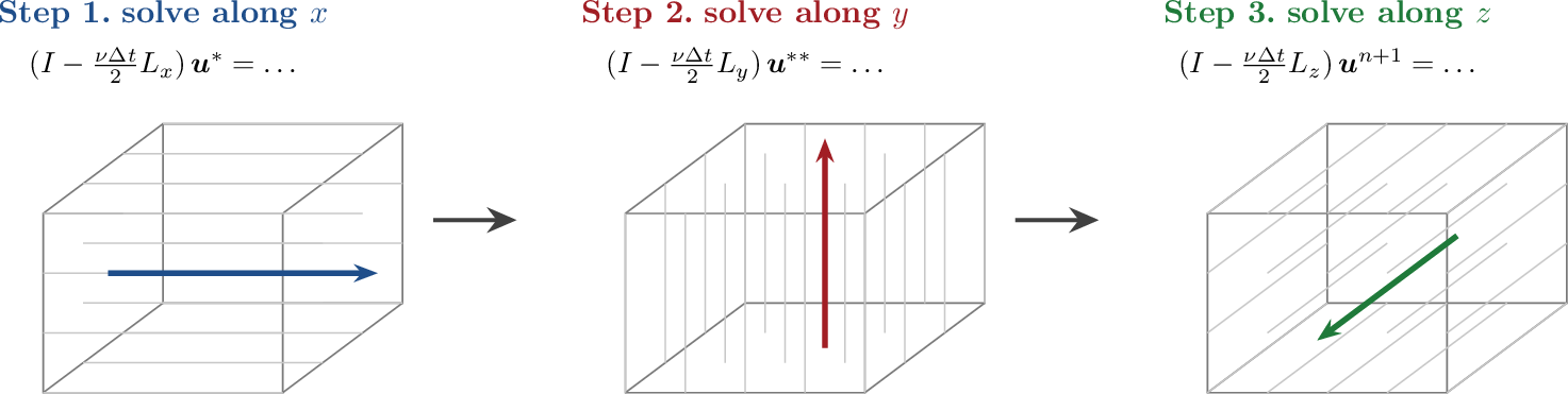
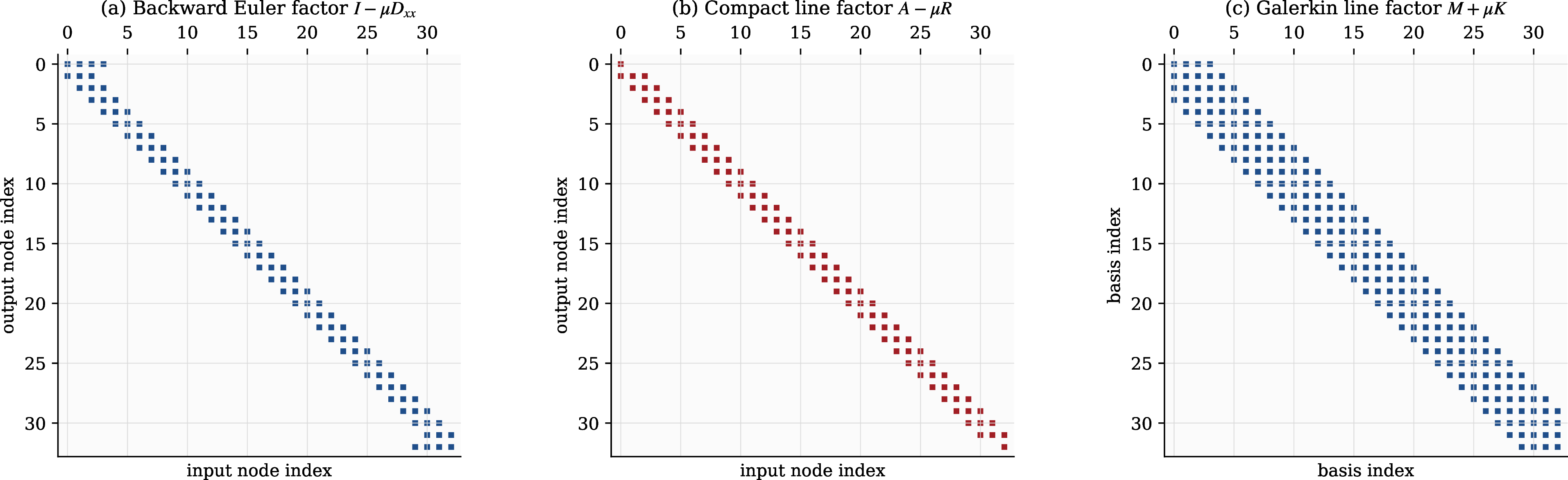
7 shows the cascade pictorially: the coupled 3D solve unravels, direction by direction, into banded line solves. 8 shows the one-dimensional factors themselves: explicit finite differences give backward Euler factors \(I - \tfrac{\nu\Delta t}{2}D_{xx}\) directly, compact schemes give banded factors \(A_{xx}- \tfrac{\nu\Delta t}{2}R_{xx}\) after moving the compact mass to the operator side, and Galerkin and spline methods give factors \(M_x + \tfrac{\nu\Delta t}{2}K_x\) that are banded because their 1D ingredients are.
8.1 The splitting↩︎
For the heat equation \(\partial u/\partial t = \nu \nabla^2 u\) with diffusivity \(\nu\), the semi-discrete system is \(\dot{\boldsymbol{u}} = \nu\Delta_h\boldsymbol{u}\) and a backward-Euler step is \[\label{eq:backward-euler} (I - \nu\,\Delta t\,\Delta_h)\;\boldsymbol{u}^{n+1} = \boldsymbol{u}^n.\tag{29}\] The matrix on the left is \(N\times N\). Factoring it head-on would defeat the whole enterprise. The trick is to remember that \(\Delta_h= L_x + L_y + L_z\) with \[L_x = I_{z}\otimes I_{y}\otimes D_{xx}, \quad L_y = I_{z}\otimes D_{yy}\otimes I_{x}, \quad L_z = D_{zz}\otimes I_{y}\otimes I_{x},\] and to solve with each piece in turn. The Douglas–Gunn splitting [18], written here in its Crank–Nicolson form, is the scheme of choice. Set \(r = \nu\Delta t/2\); the three substeps are \[\begin{align} (I - r\,L_x)\;\boldsymbol{u}^* &= \bigl(I + r\,L_x + 2r\,L_y + 2r\,L_z\bigr)\,\boldsymbol{u}^n, \tag{30} \\ (I - r\,L_y)\;\boldsymbol{u}^{**} &= \boldsymbol{u}^* - r\,L_y\,\boldsymbol{u}^n, \tag{31} \\ (I - r\,L_z)\;\boldsymbol{u}^{n+1} &= \boldsymbol{u}^{**} - r\,L_z\,\boldsymbol{u}^n. \tag{32} \end{align}\] The first-step right-hand side \((I + r L_x + 2r(L_y + L_z))\) is the Douglas–Gunn correction that makes the three substeps combine to the full Crank–Nicolson update \((I - r\Delta_h)\,\boldsymbol{u}^{n+1} = (I + r\Delta_h)\,\boldsymbol{u}^n\) modulo a splitting error of order \(\mathcal{O}((\nu\Delta t)^3)\) per step [18]; dropping the \(2r(L_y + L_z)\,\boldsymbol{u}^n\) correction collapses the scheme to \(\mathcal{O}(\Delta t)\) accuracy and biases the heat operator toward the \(x\)-direction. Each substep is a banded 1D solve because, under the identity from 14.3 plus distributivity, the \(x\)-substep operator is \[I - \tfrac{\nu\Delta t}{2}\,L_x \;=\; I_{z}\otimes I_{y}\otimes\bigl(I_{x}- \tfrac{\nu\Delta t}{2}\,D_{xx}\bigr),\] and the bracketed 1D factor is tridiagonal. The \(y\)- and \(z\)-substeps factor identically in their own directions. Each substep therefore costs \(\mathcal{O}(N)\) in the Thomas algorithm, so the whole implicit step is \(\mathcal{O}(N)\) with a modest constant, the same asymptotic cost as one explicit sweep.
8.2 The same splitting for every discretization↩︎
Changing the discretization changes the \(1\)D factor, not the outer Kronecker structure. A sixth-order compact scheme, where \(D_{xx}= A_{xx}^{-1}R_{xx}\), produces the line factor \[A_{xx}- \tfrac{\nu\Delta t}{2}R_{xx},\] tridiagonal because tridiagonals subtract. A Galerkin or B-spline semi-discretization \(M\dot{\boldsymbol{u}} = -K\boldsymbol{u}\) produces \[M_x + \tfrac{\nu\Delta t}{2} K_x,\] banded because both \(M_x\) and \(K_x\) are banded. B-spline collocation in coefficient form produces \[B_x - \tfrac{\nu\Delta t}{2}\,B_x'',\] banded because both \(B_x\) and \(B_x''\) are. In every case each ADI substep is a banded 1D solve; only the bandwidth and the entries change. The same splitting also covers the advection-diffusion equation \(\partial_t u + \boldsymbol{c}\cdot\nabla u = \nu\nabla^2 u\) with \(L_\xi = c_\xi D_\xi + \nu D_{\xi\xi}\), and any equation whose spatial operator decomposes cleanly along the coordinate axes.
9 Direct Poisson solvers via fast diagonalization↩︎
There is a second, complementary payoff of the Kronecker structure. For constant-coefficient separable problems, in particular the Poisson equation \(\Delta_h\,\boldsymbol{u} = \boldsymbol{f}\) and shifted Helmholtz equations of the form \((\alpha I + \beta\Delta_h)\,\boldsymbol{u} = \boldsymbol{f}\) that arise inside implicit time stepping, the same algebra gives a direct solver with no iteration at all. The idea is due to [19]: if the one-dimensional second-derivative matrices can be diagonalized, then diagonalizing each direction in turn decouples the 3D problem into independent scalar divisions. For Chebyshev expansions, the companion construction is [20]. The eigenbases themselves are computed once as a preprocessing step and reused on every solve, so the expensive part happens only at setup time.
9.1 Diagonalize each direction, add the eigenvalues↩︎
Suppose each 1D second-derivative matrix is diagonalizable, \[D_{xx}= S_x \Lambda_x S_x^{-1}, \quad D_{yy}= S_y \Lambda_y S_y^{-1}, \quad D_{zz}= S_z \Lambda_z S_z^{-1},\] with \(\Lambda_\xi = \operatorname{diag}(\lambda_1^\xi, \ldots, \lambda_{N_\xi}^\xi)\). Substituting into the Laplacian, applying the mixed-product rule three times, and transforming \(\boldsymbol{u}\) and \(\boldsymbol{f}\) into the tensor-product eigenbasis \(\hat{\boldsymbol{u}} = (S_z^{-1} \otimes S_y^{-1} \otimes S_x^{-1})\boldsymbol{u}\) leaves the Poisson problem diagonal (14.4): \[\label{eq:poisson-diag} \boxed{ \hat{u}_{ijk} \;=\; \frac{\hat{f}_{ijk}}{\lambda_i^x + \lambda_j^y + \lambda_k^z}. }\tag{33}\] The 3D Poisson solve has become a scalar division at every grid point. Adding the three eigenvalues is the whole algorithm. When a denominator is zero, as in a pure Neumann Poisson problem, the usual compatibility condition must hold and the zero mode is fixed by a normalization such as zero mean.

The bookkeeping around that scalar division is three transforms and their inverses: apply \(S_x^{-1}\) along all \(x\)-lines, then \(S_y^{-1}\) along all \(y\)-lines, then \(S_z^{-1}\) along all \(z\)-lines to get \(\hat{\boldsymbol{f}}\); divide pointwise; apply the forward transforms in reverse (9). For a uniform grid the eigenvectors are trigonometric and the boundary condition, grid placement, and endpoint closure select the appropriate member of the standard transform families: discrete sine transforms for homogeneous Dirichlet boundaries, discrete cosine transforms for homogeneous Neumann boundaries, and the discrete Fourier transform for periodic boundaries. Each of these costs \(\mathcal{O}(N_\xi \log N_\xi)\) per line and \(\mathcal{O}(N\log N_{\max})\) overall, and all are available in optimized form (for instance through FFTW [26]). On stretched or Chebyshev grids the eigenvectors are not generally trigonometric; the transforms become small dense matrix products at \(\mathcal{O}(N_\xi^2)\) per line and \(\mathcal{O}(NN_{\max})\) overall, still far below the cost of factoring the full 3D operator [20]. A shifted problem \((\alpha I+\beta\Delta_h)\boldsymbol{u}=\boldsymbol{f}\) is handled at zero conceptual extra cost by replacing the denominator in 33 with \(\alpha+\beta(\lambda_i^x+\lambda_j^y+\lambda_k^z)\), provided that quantity never vanishes except for modes fixed by the compatibility condition.
10 Applicability of the tensor-product reduction↩︎
The right question is not whether a problem is “three-dimensional.” Every problem in this paper is three-dimensional. The right question is whether the algebra can be written as a small sum of tensor products, \[\label{eq:applicability-kron-sum} L = \sum_{r=1}^{R} C_z^{(r)} \otimes C_y^{(r)} \otimes C_x^{(r)}.\tag{34}\] When \(R\) is small and each one-dimensional factor is banded, diagonal, or transformable, the whole machinery applies. A single derivative sweep has \(R=1\) with two identity factors. The Cartesian Laplacian has \(R=3\). A separable coefficient such as \(a(x,y,z)=a_x(x)a_y(y)a_z(z)\) simply inserts diagonal one-dimensional factors into the same product.
This criterion is the clean line between the exact reduction and the many useful extensions of it. Tensor-product grids and tensor-product bases give the reduction natively. Problems with additional nonseparable physics still benefit from the same 1D solvers as split operators, fast preconditioners, or patchwise kernels. The table below is therefore a map of where the reduction is exact and where it becomes the computational backbone inside a larger solver.
| Setting | Role of the tensor-product reduction |
|---|---|
| Uniform Cartesian | Exact. The simplest case, with identical 1D factors reused on every line. |
| Non-uniform Cartesian | Exact. Spacing varies per direction, but the grid is still a tensor product of 1D grids. |
| Stretched or clustered grids | Exact. Wall clustering, tanh maps, and biased spacing only change the 1D weights. |
| Mixed boundary conditions | Exact. Different boundary closures are absorbed into the endpoint rows of the 1D operators. |
| Galerkin tensor-product basis | Exact. Mass and stiffness matrices inherit the Kronecker structure of the basis. |
| B-spline and IGA patches | Exact on tensor-product patches. The same factorization holds for spline mass, stiffness, and collocation maps. |
| B-spline collocation | Exact in factorized form. Use banded maps \(B\), \(B'\), and \(B''\) rather than preformed dense products such as \(B''B^{-1}\). |
| Separable variable coefficients | Exact. Products such as \(a_x(x)a_y(y)a_z(z)\) preserve 34 . |
| General variable coefficients | Core solver component. The separable or constant-coefficient part remains a fast split operator or preconditioner; the remaining coupling is handled matrix-free, iteratively, or by a low-rank separated approximation when such an approximation is accurate. |
| Curvilinear grids | Exact when the metrics separate, otherwise patchwise. General metric terms add couplings, while tensor-product blocks still supply fast local kernels and preconditioners. |
| Unstructured grids | Indirect. There are no global grid lines, but tensor-product elements, blocks, and patches retain the same dimension-by-dimension kernels locally. |
11 How production codes actually run: multi-RHS kernels, sum factorization, and pencils↩︎
So far the paper has argued that a three-dimensional Cartesian operator factors into a loop of one-dimensional line kernels. That argument is complete at the algebraic level. But a graduate student writing a research code should know the three practical tricks that separate a textbook implementation of the same loop from a production one running near peak floating-point rate. These tricks are almost never written down in one place. They are the reason high-order CFD and spectral-element codes achieve their reputations for efficiency.
11.1 Trick 1: reshape a sweep into a multi-right-hand-side line kernel↩︎
Consider the \(x\)-sweep \(v_{ijk} = \sum_{\ell} (D_{x})_{i\ell}\, u_{\ell j k}\). Naively this is \(N_y N_z\) separate line operations, each of size \(N_x\). That is the right mathematical kernel but the wrong software shape: the operator data, boundary rows, and factorizations are reused across many lines, yet a scalar loop exposes only one right-hand side at a time.
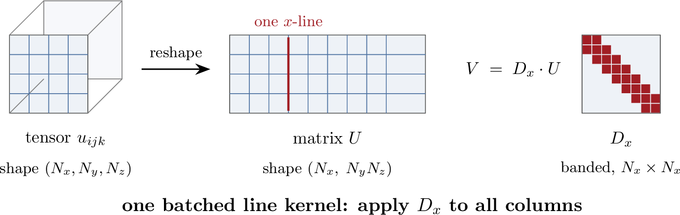
10 shows the production trick: reshape the tensor \(u \in \mathbb{R}^{N_x \times N_y \times N_z}\) into a matrix \(U \in \mathbb{R}^{N_x \times (N_y N_z)}\), whose columns are the \(x\)-lines. The line apply is then the multi-right-hand-side operation \[\label{eq:blas3} V \;=\; D_{x}\, U.\tag{35}\] Equation 35 should be read with one important implementation caveat. If \(D_{x}\) is dense, spectral, or element-local and small, this is exactly the shape of a BLAS-3 GEMM call. If \(D_{x}\) is a narrow finite-difference stencil, densifying it would change the work from \(\mathcal{O}(w_xN)\) to \(\mathcal{O}(N_xN)\) and destroy the point of the method. In that case, the correct production kernel is a banded multi-RHS apply or a hand-written stencil kernel over the columns of \(U\). Compact and Galerkin line solves use the solve analog: factor the one-dimensional banded matrix once, then apply the factors to many right-hand sides at once. The same reshape works for the \(y\)- and \(z\)-sweeps after a transpose or stride adjustment that places the active direction first; see 5.5 for the data-layout side of the argument.
11.1.0.1 Why this matters.
The reshape is the single most important reason production Cartesian codes look fast. It exposes reuse across many lines, lets dense or element-local pieces fall into optimized GEMM, and lets banded pieces use batched line kernels instead of scalar loops. The linear-algebraic content is unchanged; only the loop order and memory layout are different. Once the right kernel is chosen for the bandwidth at hand, this reshape is essentially free.
11.2 Trick 2: sum factorization (the spectral-element secret)↩︎
A related, more dramatic speedup governs tensor-product Galerkin and spectral-element methods at high polynomial order \(p\). The right-hand-side quadrature sum on one element of \((p+1)^d\) points in \(d\) dimensions is \[F_{abc} \;=\; \sum_{q_1, q_2, q_3} w_{q_1 q_2 q_3}\, \phi_a(\xi_{q_1})\, \phi_b(\eta_{q_2})\, \phi_c(\zeta_{q_3})\, f(\xi_{q_1}, \eta_{q_2}, \zeta_{q_3}).\] If you read this literally, every one of the \((p+1)^3\) outputs sums over \((p+1)^3\) inputs. With \(n=p+1\) points per direction, that is \(\mathcal{O}(n^{2d}) = \mathcal{O}(n^{6})\) operations per element in 3D. For \(p=8\) (\(n=9\)), the naive count is about \(5.3\times10^5\) multiply-adds per element; for \(p=16\) (\(n=17\)), it is about \(2.4\times10^7\). This is the scaling that kept high-order methods out of production engineering for two decades.
The cure lives in the same separation of variables that ran the rest of the paper. Do not sum all three indices at once; sum one at a time. Contract \(q_3\) with \(\phi_c\) to make an intermediate of shape \((p{+}1)^2 \times (p{+}1)\); then contract \(q_2\) with \(\phi_b\); then contract \(q_1\) with \(\phi_a\): \[\label{eq:sumfac} F_{abc} \;=\; \sum_{q_1} \phi_a(\xi_{q_1}) \underbrace{ \sum_{q_2} \phi_b(\eta_{q_2}) \underbrace{ \sum_{q_3} \phi_c(\zeta_{q_3})\, w_{q_1 q_2 q_3}\, f_{q_1 q_2 q_3} }_{\text{cost } \mathcal{O}(n^{4})} }_{\text{cost } \mathcal{O}(n^{4})} \qquad\text{(and one more outer sum)}.\tag{36}\] Each contraction costs \((p{+}1)^3 \times (p{+}1) = \mathcal{O}(n^{4})\). Three contractions, three directions. The total drops from \(\mathcal{O}(n^{2d})\) to \(\mathcal{O}(d\, n^{d+1})\), which is \(\mathcal{O}(n^{4})\) in 3D. Including the three contractions, the leading-count speedup is about \(n^2/3\): roughly \(27\times\) at \(p=8\) and \(96\times\) at \(p=16\) (11). This is why spectral-element and high-order DG codes can run at orders that would otherwise be unthinkable [4]. In Kronecker notation, 36 is the contraction \(F = (\Phi_\xi \otimes\Phi_\eta \otimes\Phi_\zeta)^T (W\odot f)\), evaluated as three sequential 1D matrix multiplies rather than as one Kronecker-product matvec. It is the same factorization that ran the derivatives, the mass inversion, and the ADI substeps, applied now to the quadrature loop itself.

11.3 Trick 3: pencil decomposition for parallel execution↩︎
The serial story only takes us so far. On a cluster of thousands of MPI ranks, one direction of the grid will always be scattered across ranks, and a sweep in that direction must move data. The cleanest response is the pencil decomposition: lay the MPI ranks on a two-dimensional process grid of size \(P_\alpha \times P_\beta\), so that the third direction lives entirely on each rank as a long “pencil” of unknowns. Before each sweep, a collective transpose rotates the pencil orientation so that the direction about to be swept is the local one (12). A full three-direction sweep therefore uses two all-to-all transposes; the third orientation can often be reused for the next time step.
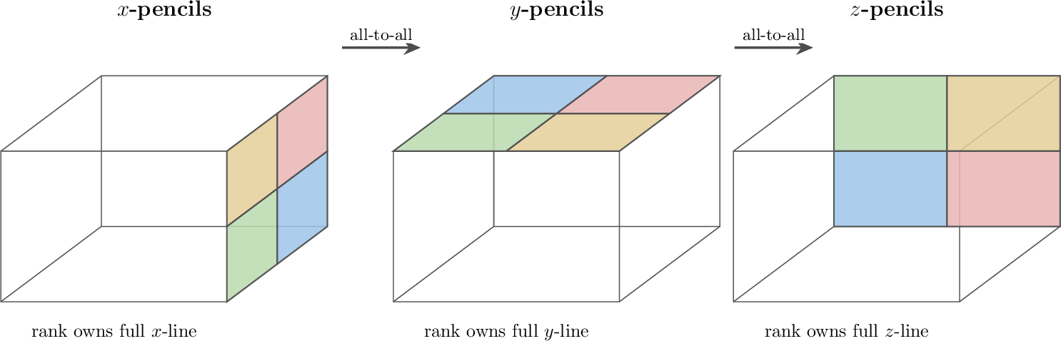
The FFT-based DNS solver CaNS [3] and the 2DECOMP&FFT pencil-decomposition library [5], [6] both follow this pattern. The pencil decomposition is the parallel analog of the serial
transpose that turns a \(y\)- or \(z\)-sweep into a contiguous kernel (5.5). At both scales the idea is the same: the tensor-product grid factors, and the
algorithm is free to factor with it.
11.4 Three tricks, one idea↩︎
The three tricks are one idea seen at three scales. The multi-RHS reshape exposes \(N_y N_z\) line operations as one batched kernel because the stride pattern of a sweep is separable in \((i,j,k)\). The sum factorization collapses \(\mathcal{O}(n^{2d})\) integrals into \(\mathcal{O}(d\,n^{d+1})\) because the quadrature kernel is separable in \((q_1,q_2,q_3)\). The pencil decomposition collapses a distributed sweep into a local one, with a transpose before and after, because the data layout is separable across the MPI ranks. Every speedup recovers the same separable structure the PDE always had, at a scale the linear algebra alone could not reach.
This is also the right design rule for software. A Cartesian PDE code should choose an active direction, expose all lines in that direction as the columns of a matrix, apply the one-dimensional operator or solve to all columns at once, and then rotate the layout for the next direction. The apparent bookkeeping around reshapes, transposes, and MPI collectives is not auxiliary machinery; it is the mechanism that lets the mathematical factorization survive contact with memory hierarchy and distributed hardware. Once this rule is followed, the same source-level idea covers finite differences, compact schemes, spline Galerkin methods, ADI steps, and FFT Poisson solvers.
12 A numerical illustration: assembled versus matrix-free↩︎
The cost argument is easy to state and easy to check. We solve the Poisson problem \(-\nabla^2 u = g\) on the unit cube with homogeneous Dirichlet boundaries and the manufactured solution \(u = \sin(\pi x)\sin(\pi y)\sin(\pi z)\), discretized by the standard seven-point stencil on an \(N\times N\times N\) interior grid, and solve the same discrete system two ways. The assembled route forms the monolithic sparse Laplacian of size \(N^3\times N^3\) as the Kronecker sum 20 and factors it with a sparse direct solver. The matrix-free route never builds that matrix: it solves by fast diagonalization (9)—a discrete sine transform along each axis, a pointwise division by \(\lambda_i^x+\lambda_j^y+\lambda_k^z\), and an inverse transform. Because both routes solve the identical discrete system, any difference is in storage and run time, not in the answer.
| assembled direct solve | matrix-free fast diag. | |||||
|---|---|---|---|---|---|---|
| 3-4(lr)5-6 \(N\) | unknowns \(N^3\) | factor (MB) | time (s) | storage (KB) | time (s) | \(\|u_h-u\|_\infty\) |
| \(16\) | \(4{,}096\) | \(14.8\) | \(0.08\) | \(0.38\) | \(0.0001\) | \(2.8\times10^{-3}\) |
| \(32\) | \(32{,}768\) | \(385\) | \(3.45\) | \(0.77\) | \(0.0006\) | \(7.5\times10^{-4}\) |
| \(48\) | \(110{,}592\) | \(2{,}799\) | \(55.4\) | \(1.15\) | \(0.0022\) | \(3.4\times10^{-4}\) |
| \(64\) | \(262{,}144\) | infeasible | \(1.54\) | \(0.0044\) | \(2.0\times10^{-4}\) | |
| \(128\) | \(2{,}097{,}152\) | infeasible | \(3.07\) | \(0.073\) | \(4.9\times10^{-5}\) | |
| \(256\) | \(16{,}777{,}216\) | infeasible | \(6.14\) | \(1.98\) | \(1.2\times10^{-5}\) | |
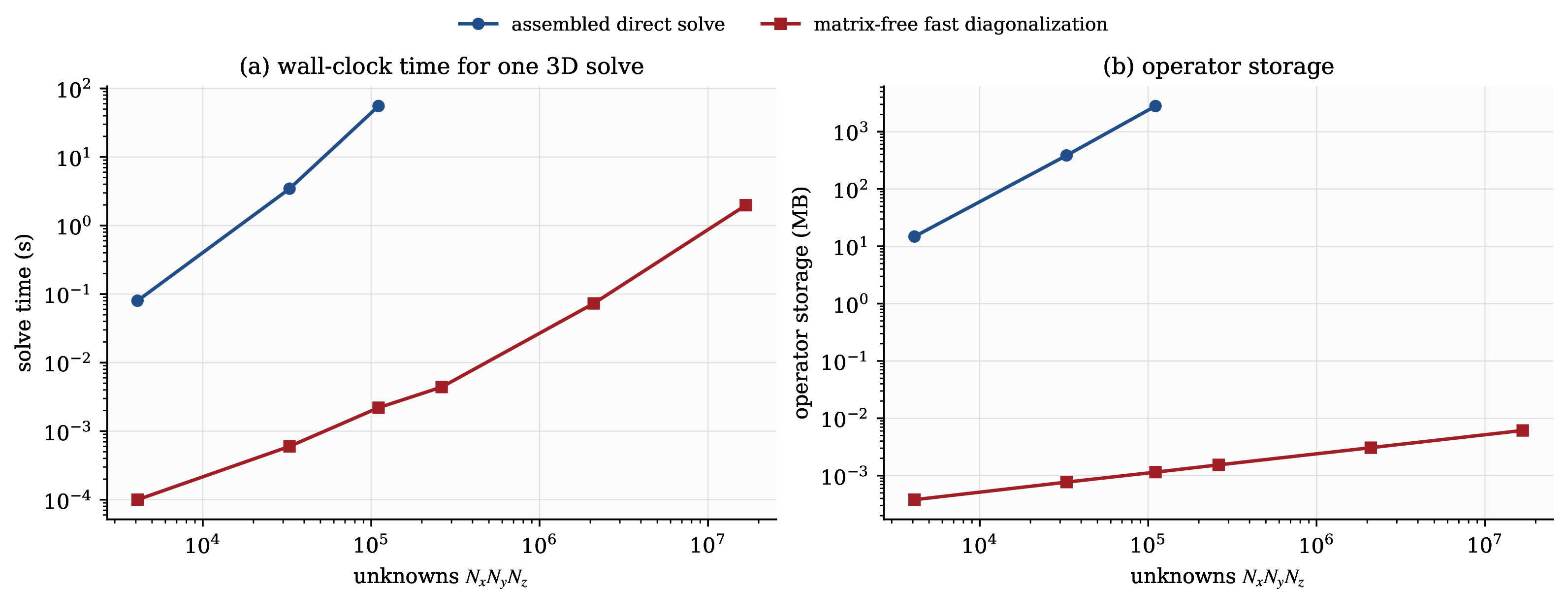
The numbers make three points. First, the matrix-free route costs no accuracy: the two solutions are the same discrete field to roughly \(10^{-14}\), and both converge at second order. Second, the assembled route pays for the three-dimensional matrix through fill-in. At \(48^3 \approx 1.1\times10^{5}\) unknowns its sparse factor already needs about \(2.8\) GB, whereas the matrix-free operator is the set of one-dimensional eigenvalues, about one kilobyte—a storage ratio above two million. Third, that fill-in is also a time wall: the direct factorization takes nearly a minute at \(48^3\) and exhausts a workstation beyond it, while the matrix-free solver clears \(256^3\), about seventeen million unknowns, in roughly two seconds. The \(\mathcal{O}(N)\) storage and \(\mathcal{O}(N\log N_{\max})\) work claimed throughout this paper are not asymptotic promises; they are visible at ordinary grid sizes.
12.0.0.1 Code availability.
The scripts that regenerate every figure and 2 in this paper, together with the LaTeX source, are available at https://github.com/bay-yearick-lab/no-3d-matrices.
13 Summary and implementation recipe↩︎
The practical conclusion of the paper fits on one page. Let \(N= N_x N_y N_z\) denote the total number of unknowns. The central result is this: every local tensor-product derivative sweep and every factorized tensor-product line solve costs \(\mathcal{O}(N)\) and stores only the one-dimensional banded operators.
Build 1D operators. Construct \(D_{x}\), \(D_{xx}\) (and \(A_{x}\), \(R_{x}\) for compact schemes) in each direction. For Galerkin or B-spline methods, build the 1D mass matrices \(M_x\), \(M_y\), \(M_z\) and stiffness matrices \(K_x\), \(K_y\), \(K_z\). For spline collocation, build the banded nodal maps \(B_x\), \(B_x'\), \(B_x''\) rather than relying on a formed product such as \(B_x'' B_x^{-1}\). These are all small banded matrices of sizes \(N_x\), \(N_y\), \(N_z\).
Evaluate derivatives by sweeping lines. To compute \(\partial u/\partial x\): make the \(x\)-direction contiguous and apply \(D_{x}\) to every \(x\)-line. The \(y\)- and \(z\)-directions follow by relabeling. For compact schemes each line operation is a banded matvec plus a banded solve. For Galerkin and spline discretizations, use the factorized banded maps along each line. The full sweep costs \(\mathcal{O}(N)\). For production performance, issue each sweep as one batched line kernel on the reshape \((N_\xi) \times (N/ N_\xi)\); use dense BLAS only when the one-dimensional factor is dense or element-local (11.1).
Implicit time stepping with ADI. Split the implicit operator direction by direction. Each substep is a batch of 1D banded solves, making the implicit method asymptotically the same cost as explicit, namely \(\mathcal{O}(N)\) per time step. The line factors are \(I - \tfrac{\nu\Delta t}{2}D_{xx}\) for finite differences, \(A_{xx}- \tfrac{\nu\Delta t}{2}R_{xx}\) for compact schemes, and \(M_x + \tfrac{\nu\Delta t}{2}K_x\) for Galerkin and spline methods. Every one of them is banded.
Direct Poisson and Helmholtz solves. Eigendecompose the 1D operators once at setup, transform direction by direction, solve pointwise, transform back. When the 1D eigenvectors are trigonometric (uniform grid with Dirichlet, Neumann, or periodic boundaries), the transforms are FFTs and the total cost is \(\mathcal{O}(N\log N_{\max})\). In general the transforms are small dense products per line.
Scale up. For large problems, parallelize with a pencil decomposition (11.3) so every direction can be made contiguous in turn by a collective transpose. For high-order Galerkin or spectral-element methods, evaluate every quadrature sum by sum factorization (11.2) to replace the \(\mathcal{O}(n^{2d})\) trap with the \(\mathcal{O}(d\,n^{d+1})\) reality, where \(n=p+1\) is the number of points per direction.
For fixed stencil width or fixed polynomial degree, local sweeps and factorized line solves cost \(\mathcal{O}(N)\) arithmetic and require only \(\mathcal{O}(N_x+N_y+N_z)\) operator storage, in addition to the \(\mathcal{O}(N)\) storage for the fields themselves. Direct separable Poisson and Helmholtz solvers add transform costs, typically \(\mathcal{O}(N\log N_{\max})\) with FFT-type bases. The line operations fan out across cores without coupling inside a sweep, fit naturally into cache and accelerator memory hierarchies, and are exactly the shape targeted by batched banded solvers and dense BLAS kernels when the one-dimensional factors are dense or element-local. Classical textbooks arrive at related algorithms by different roads [27]–[29]; the route taken here is the Kronecker product, which trades a page of index gymnastics for a single line of algebra and gives a sharp baseline against which matrix-free, low-rank, and learned accelerators can be judged. For learned accelerators the test is twofold—cost against this \(\mathcal{O}(N)\) baseline, and accuracy once the inputs drift away from the training regime, where the distinction between fitting and genuine generalization becomes decisive [30].
13.0.0.1 A closing word.
A separable three-dimensional Cartesian problem is really a one-dimensional problem, dressed up for a Cartesian grid. The operator respects that product structure; the data layout, the line kernel, and the parallel decomposition do too; and none of them ever needs to see the monolithic three-dimensional matrix whose existence caused the alarm in the first place. When the Kronecker product, the word “line,” and the phrase “banded solve” are held in the same sentence, the picture is complete. Every discretization family this paper surveyed obeys it. Long an unwritten habit of specialist codes, it is elementary once the Kronecker product is taken as the organizing principle.
14 Algebraic details for the 1D reductions↩︎
The main text uses the Kronecker product as a language for loops. This appendix gives the short, self-contained derivations that translate that language back into arrays, line solves, and direct diagonalization formulas. The whole edifice rests on two identities: the mixed-product rule of 14.1, and the vec identity of 14.2. Every subsequent derivation in this appendix is one or two applications of one or both.
14.1 Mixed-product rule and Kronecker inverse↩︎
14.1.0.1 Claim.
For matrices \(A \in \mathbb{R}^{m \times n}\), \(C \in \mathbb{R}^{n \times \ell}\), \(B \in \mathbb{R}^{p \times q}\), \(D \in \mathbb{R}^{q \times r}\), \[\label{eq:mixed-product-app} (A \otimes B)(C \otimes D) \;=\; (AC) \otimes(BD).\tag{37}\]
14.1.0.2 Proof.
By block matrix multiplication, the \((i,k)\) block of a product of two block matrices is \(\sum_{j} (\text{block}_{ij}^{(1)})\,(\text{block}_{jk}^{(2)})\). By definition of the Kronecker product, the \((i,j)\) block of \(A \otimes B\) is the scalar-times-matrix \(a_{ij}\,B\), and similarly the \((j,k)\) block of \(C \otimes D\) is \(c_{jk}\,D\). The \((i,k)\) block of the left-hand side of 37 is therefore \[\sum_{j=1}^{n} (a_{ij}\,B)(c_{jk}\,D) \;=\; \sum_{j=1}^{n} a_{ij}\, c_{jk}\, B\, D \;=\; \biggl(\sum_{j=1}^{n} a_{ij}\,c_{jk}\biggr) B\, D \;=\; (AC)_{ik}\,(BD),\] where the second equality uses the fact that \(a_{ij}\) and \(c_{jk}\) are scalars and slide through \(B\) and \(D\) freely. The right-hand side is the \((i,k)\) block of \((AC) \otimes(BD)\), which establishes 37 . \(\square\)
14.1.0.3 Corollary (inverse rule).
If \(A\) and \(B\) are square and invertible, take \(C = A^{-1}\) and \(D = B^{-1}\) in 37 : \[(A \otimes B)(A^{-1} \otimes B^{-1}) \;=\; (A A^{-1}) \otimes(B B^{-1}) \;=\; I_m \otimes I_p \;=\; I_{mp},\] and the product taken in the other order yields \(I_{mp}\) as well, so the inverse is two-sided. Hence \[\label{eq:kron-inv-app} (A \otimes B)^{-1} \;=\; A^{-1} \otimes B^{-1}.\tag{38}\] The triple-product extension follows by associativity: \((A \otimes B \otimes C)^{-1} = A^{-1} \otimes B^{-1} \otimes C^{-1}\) whenever each factor is square and invertible.
14.2 The vec identity (master lemma)↩︎
Throughout the paper, \(\operatorname{vec}\) uses the column-major convention. For \(U \in \mathbb{R}^{m \times n}\) with columns \(U_{:,1}, U_{:,2}, \ldots, U_{:,n}\), \[\label{eq:vec-def} \operatorname{vec}(U) \;=\; \begin{bmatrix} U_{:,1} \\[2pt] U_{:,2} \\[2pt] \vdots \\[2pt] U_{:,n} \end{bmatrix} \;\in\; \mathbb{R}^{mn}.\tag{39}\] The columns of \(U\) stack vertically into one tall column vector. Reading \(\operatorname{vec}(U)\) from top to bottom walks the row index (\(x\)) fastest and the column index (\(y\)) slowest, which is the ordering used throughout the main text.
14.2.0.1 Claim (vec identity).
For \(A \in \mathbb{R}^{m \times m}\), \(B \in \mathbb{R}^{n \times n}\), and \(X \in \mathbb{R}^{m \times n}\), \[\label{eq:vec-identity} \boxed{\,(B^T \otimes A)\,\operatorname{vec}(X) \;=\; \operatorname{vec}(A X B).\,}\tag{40}\]
14.2.0.2 Proof.
Write \(Y = A X B\). Using \(B_{:,j} = \sum_k B_{kj}\,e_k\) where \(e_k\) is the \(k\)th standard basis vector and \(X e_k = X_{:,k}\), the \(j\)th column of \(Y\) is \[Y_{:,j} \;=\; A\, X\, B_{:,j} \;=\; A\,\sum_{k=1}^{n} B_{kj}\, X_{:,k} \;=\; \sum_{k=1}^{n} B_{kj}\,(A\, X_{:,k}).\] Stacking the columns of \(Y\) in column-major order gives \[\operatorname{vec}(Y) \;=\; \begin{bmatrix} \sum_{k} B_{k 1}\, A\, X_{:,k} \\[2pt] \sum_{k} B_{k 2}\, A\, X_{:,k} \\[2pt] \vdots \\[2pt] \sum_{k} B_{k n}\, A\, X_{:,k} \end{bmatrix}.\] This vector is exactly \((B^T \otimes A)\,\operatorname{vec}(X)\) read by blocks: the \(j\)th block is \(\sum_k (B^T)_{j k}\, A\, X_{:,k} = \sum_k B_{k j}\, A\, X_{:,k}\), as required. \(\square\)
Two specializations of 40 carry most of the computational weight in the main text. Setting \(B = I_n\) kills the right multiplication and gives \[\label{eq:vec-IA} (I_n \otimes A)\,\operatorname{vec}(X) \;=\; \operatorname{vec}(A X).\tag{41}\] Setting \(A = I_m\) instead, and writing \(\tilde{B} = B^T\), gives \[\label{eq:vec-BI} (\tilde{B} \otimes I_m)\,\operatorname{vec}(X) \;=\; \operatorname{vec}(X\, \tilde{B}^T).\tag{42}\] In words: 41 says a matrix in the rightmost Kronecker slot acts down the columns of the array form of \(\operatorname{vec}(X)\); 42 says a matrix in the next slot acts across the rows. These two statements are the entire algebraic content of the 2D line-sweep picture.
14.3 The 3D directional actions↩︎
In three dimensions, store the field as \(U(:,:,:) \in \mathbb{R}^{N_x \times N_y \times N_z}\) with the \(x\)-index first. Write \(U^{(k)} = U(:,:,k) \in \mathbb{R}^{N_x \times N_y}\) for the \(k\)th \(x\)-\(y\) plane. The flattened vector \(\boldsymbol{u} \in \mathbb{R}^{N}\) is built by stacking the columns within each plane, then stacking the planes: \[\label{eq:3d-flat} \boldsymbol{u} \;=\; \begin{bmatrix} \operatorname{vec}(U^{(1)}) \\[2pt] \operatorname{vec}(U^{(2)}) \\[2pt] \vdots \\[2pt] \operatorname{vec}(U^{(N_z)}) \end{bmatrix} \;\in\; \mathbb{R}^{N}.\tag{43}\] With this convention, \(x\) varies fastest, then \(y\), then \(z\). The three directional actions of the main text follow immediately from the 2D specializations 41 –42 applied plane by plane.
14.3.0.1 \(x\)-direction.
The outer factor \(I_{z}\) leaves the plane index \(k\) untouched, so the \(k\)th block of \((I_{z}\otimes I_{y}\otimes D_{x})\,\boldsymbol{u}\) is \((I_{y}\otimes D_{x})\,\operatorname{vec}(U^{(k)})\). By 41 this equals \(\operatorname{vec}(D_{x}\,U^{(k)})\), which gives \[\label{eq:app-x-action} (I_{z}\otimes I_{y}\otimes D_{x})\,\boldsymbol{u} \;=\; \begin{bmatrix} \operatorname{vec}(D_{x}\,U^{(1)}) \\[2pt] \vdots \\[2pt] \operatorname{vec}(D_{x}\,U^{(N_z)}) \end{bmatrix}.\tag{44}\] The interpretation is the line sweep: apply \(D_{x}\) to every column of every plane.
14.3.0.2 \(y\)-direction.
The \(k\)th block of \((I_{z}\otimes D_{y}\otimes I_{x})\,\boldsymbol{u}\) is \((D_{y}\otimes I_{x})\,\operatorname{vec}(U^{(k)})\). By 42 with \(\tilde{B} = D_{y}\) this equals \(\operatorname{vec}(U^{(k)}\,D_{y}^T)\), so \[\label{eq:app-y-action} (I_{z}\otimes D_{y}\otimes I_{x})\,\boldsymbol{u} \;=\; \begin{bmatrix} \operatorname{vec}(U^{(1)}\,D_{y}^T) \\[2pt] \vdots \\[2pt] \operatorname{vec}(U^{(N_z)}\,D_{y}^T) \end{bmatrix}.\tag{45}\] Multiplying \(U^{(k)}\) by \(D_{y}^T\) on the right is the same as applying \(D_{y}\) along each row of \(U^{(k)}\), that is, along each \(y\)-line at fixed \(z = k\).
14.3.0.3 \(z\)-direction.
The \(D_{z}\) factor now sits on the plane index, so it produces a linear combination of whole planes: \[\label{eq:app-z-action} (D_{z}\otimes I_{y}\otimes I_{x})\,\boldsymbol{u} \;=\; \begin{bmatrix} \sum_{r=1}^{N_z} (D_{z})_{1 r}\,\operatorname{vec}(U^{(r)}) \\[2pt] \vdots \\[2pt] \sum_{r=1}^{N_z} (D_{z})_{N_z\, r}\,\operatorname{vec}(U^{(r)}) \end{bmatrix}.\tag{46}\] Equivalently, treat the matrix \(M = [\,\operatorname{vec}(U^{(1)}) \mid \operatorname{vec}(U^{(2)}) \mid \cdots \mid \operatorname{vec}(U^{(N_z)})\,] \in \mathbb{R}^{(N_x N_y) \times N_z}\), whose \(k\)th column holds the flattened plane \(U^{(k)}\). Then 46 is the matrix product \(M\,D_{z}^T\) read column by column, which is one banded matvec per \(z\)-line of length \(N_z\).
These three formulas, 44 –46 , are exactly the three sweeps of 1 and the sweep pseudocode of 2, written
without indices.
14.4 Kronecker sums and fast diagonalization↩︎
The discrete Laplacian is the Kronecker sum \[\label{eq:app-laplacian-kron-sum} L \;=\; I_{z}\otimes I_{y}\otimes D_{xx} \;+\; I_{z}\otimes D_{yy}\otimes I_{x} \;+\; D_{zz}\otimes I_{y}\otimes I_{x}.\tag{47}\] Suppose each 1D second-derivative matrix is diagonalizable as \(D_{xx}= S_x \Lambda_x S_x^{-1}\), \(D_{yy}= S_y \Lambda_y S_y^{-1}\), and \(D_{zz}= S_z \Lambda_z S_z^{-1}\). Each Kronecker term factors by the mixed-product rule applied twice. For the first term, write each identity as \(S_\xi S_\xi^{-1}\): \[\begin{align} I_{z}\otimes I_{y}\otimes D_{xx} &\;=\; (S_z S_z^{-1}) \otimes(S_y S_y^{-1}) \otimes(S_x \Lambda_x S_x^{-1}) \nonumber \\ &\;=\; (S_z \otimes S_y \otimes S_x)\, (I_{z}\otimes I_{y}\otimes\Lambda_x)\, (S_z^{-1} \otimes S_y^{-1} \otimes S_x^{-1}), \label{eq:fastdiag-step} \end{align}\tag{48}\] where the second line is one application of 37 extended to triple products by associativity (the binary rule applies to any factorization \(XYZ = (XY)Z = X(YZ)\), so it iterates without change). The other two Kronecker terms in 47 factor identically with \(\Lambda_y\) and \(\Lambda_z\) in the appropriate slot. Crucially, all three terms share the same outer factors \(S_z \otimes S_y \otimes S_x\) and \(S_z^{-1} \otimes S_y^{-1} \otimes S_x^{-1}\), so the sum collects: \[\label{eq:fastdiag-factored} L \;=\; (S_z \otimes S_y \otimes S_x)\, \underbrace{\bigl(I_{z}\otimes I_{y}\otimes\Lambda_x \;+\; I_{z}\otimes\Lambda_y \otimes I_{x}\;+\; \Lambda_z \otimes I_{y}\otimes I_{x}\bigr)}_{\text{diagonal}}\, (S_z^{-1} \otimes S_y^{-1} \otimes S_x^{-1}).\tag{49}\] The middle factor is diagonal because each summand is a Kronecker product of diagonal matrices and is therefore diagonal, and the sum of diagonal matrices is diagonal. Its \((i,j,k)\) entry is \(\lambda_i^x + \lambda_j^y + \lambda_k^z\).
The Poisson solve \(L\,\boldsymbol{u} = \boldsymbol{f}\) therefore reduces, in the tensor-product eigenbasis \(\hat{\boldsymbol{u}} = (S_z^{-1} \otimes S_y^{-1} \otimes S_x^{-1})\,\boldsymbol{u}\), to the scalar division \[\label{eq:app-fastdiag-final} \hat{u}_{ijk} \;=\; \frac{\hat{f}_{ijk}}{\lambda_i^x + \lambda_j^y + \lambda_k^z},\tag{50}\] provided the denominator never vanishes, or else the corresponding compatibility condition is imposed and the null mode is fixed by a normalization. A shifted operator \(\alpha I + \beta L\) replaces the denominator with \(\alpha + \beta(\lambda_i^x + \lambda_j^y + \lambda_k^z)\) and is otherwise identical.
14.5 Compact and spline formulas as line systems↩︎
The compact \(x\)-derivative system in 3D, written for the vector of derivative values \(\boldsymbol{v}\), is \[(I_{z}\otimes I_{y}\otimes A_{x})\,\boldsymbol{v} \;=\; (I_{z}\otimes I_{y}\otimes R_{x})\,\boldsymbol{u}.\] Read this plane by plane. The outer \(I_{z}\) leaves the plane index untouched; on each plane, the action of \(I_{y}\otimes A_{x}\) is 41 applied with \(A = A_{x}\) and \(X = U^{(k)}\), and similarly for \(I_{y}\otimes R_{x}\). Thus for every plane index \(k\), \[\label{eq:app-compact-plane} A_{x}\, V^{(k)} \;=\; R_{x}\, U^{(k)}.\tag{51}\] Equation 51 is itself a matrix equation; reading it column by column (each column is one \(x\)-line at fixed \(y\) and \(z\)) gives the independent line systems \[\label{eq:app-compact-line} A_{x}\, v(:,j,k) \;=\; R_{x}\, u(:,j,k), \qquad j = 1, \ldots, N_y,\; k = 1, \ldots, N_z.\tag{52}\] Each line is one banded matvec by \(R_{x}\) followed by one tridiagonal solve with \(A_{x}\), executed by the Thomas algorithm of 10 –11 . The \(y\)- and \(z\)-direction compact derivatives factor identically, using 42 and the \(z\)-plane action of 46 , respectively.
The spline coefficient-recovery and weak-form derivative equations have the same structure. The 3D collocation system \((I_{z}\otimes I_{y}\otimes B_x)\,\boldsymbol{\alpha} = \boldsymbol{u}\) becomes, by 41 on each plane, \[B_x\, A^{(k)} \;=\; U^{(k)}, \qquad\text{or column-wise}\qquad B_x\, \alpha(:,j,k) \;=\; u(:,j,k),\] where \(\alpha(:,j,k)\) is the column of coefficients along the \(x\)-line at \((j,k)\). Once recovered, the derivative samples on the same line are \[u_x(:,j,k) \;=\; B_x'\,\alpha(:,j,k).\] The IGA coefficient-derivative system \[(I_{z}\otimes I_{y}\otimes M_x)\,\boldsymbol{\beta} \;=\; (I_{z}\otimes I_{y}\otimes G_x)\,\boldsymbol{\alpha}\] becomes, in the same way, \[M_x\, \beta(:,j,k) \;=\; G_x\, \alpha(:,j,k).\] In every case the multidimensional structure expands the number of independent lines, not the size or shape of the kernel. \(\square\)
References↩︎
Equal contribution. Emails:
{yongyibay,kallie.a.yearick}@gmail.com.↩︎