Conformal Orbit-Valid Trust Horizons for Equivariant World Models
June 23, 2026
Abstract
Learned world models are useful only over horizons on which their rollout error remains controlled. We study trust-horizon certification for latent world models with known group symmetries. Given a one-step latent residual and a finite-time expansion estimate, we form a raw horizon curve and calibrate it with a split-conformal multiplicative factor. On the reproducible audit set, the conformal factor is \(\gamma_\alpha=1.0\): the raw certificate is already conservative under the audit protocol. Across 50 stable audits, we observe zero anti-conservative violations, corresponding to an exact-binomial 95% upper bound of 5.8% on the violation rate. Our main structural result is that exact equivariance transports a calibrated trust-horizon curve over the group orbit: when the environment dynamics, encoder, predictor, action transform, and latent metric satisfy the stated equivariance/invariance conditions, rollout errors and trust horizons are orbit-constant. Empirically, the implemented models exhibit small orbit-transport residuals, with median 1.1% and maximum 4.1% over 14 orbit audits. The certificate is also non-vacuous (median certified-to-measured horizon ratio 0.67). A certificate-level calibration-cost study shows two complementary regimes. On a symmetric 2D substrate, equivariant, plain, and augmented models are all orbit-valid from a single calibration sector — no separation, because the substrate already makes non-equivariant baselines approximately orbit-robust. A 3D yaw audit shows the other regime: the equivariant model obtains a one-sector safe and non-vacuous orbit-valid certificate, while healthy non-equivariant baselines pay violation, slack, sharpness, or additional-sector cost. The certificate is a conservative, distributional audit rather than a global reachability guarantee, and certificate-guided subgoal spacing is not confirmed in the current 3D CEM-MPC behavior layer.
0.1 1. Introduction↩︎
1.1 Calibration is geometric. Calibration is usually treated as a statistical operation over sampled points. For equivariant world models, calibration also has geometry: once a trust-horizon certificate is valid on a representative region, exact equivariance can transport that certificate over the group orbit. This structural statement does not imply that equivariance always yields a large empirical calibration-cost advantage: on our symmetric 2D substrate, non-equivariant baselines are already approximately orbit-robust, so the realized separation is mild (Section 5).
1.2 The trust-horizon problem. Model-based planning, imagination, and self-supervision all roll a learned dynamics model forward — but every learned model degrades, and when it stops being trustworthy is rarely answered in a principled way (FF-JEPA’s \(H{=}25\) [1] is one number for one distribution). The field splits “generate pixels” (expensive) from “predict latents” (JEPA); we work in the latent regime and ask: can a latent world model certify, a priori and with finite-sample semantics, how many steps it can be trusted — and does that certificate hold across a symmetry group?
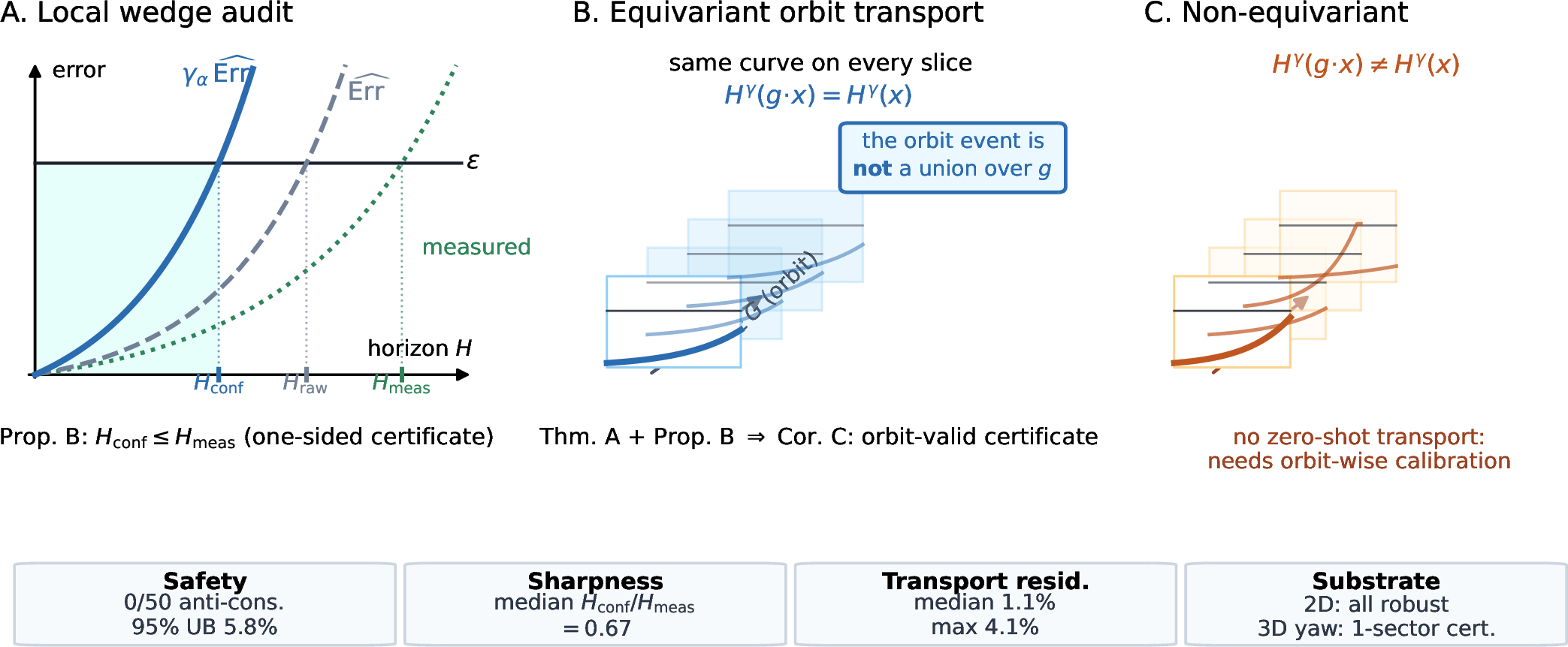
1.3 The approach. A raw error-propagation curve gives a candidate trust horizon; we make it statistically conservative by split-conformal calibration (Proposition B) and orbit-valid by equivariance (Theorem A, Corollary C) — a curve calibrated on one wedge transports over the whole group orbit at the same confidence, because equivariance turns the orbit-wide coverage event into a single calibrated event rather than a union over transformations. A non-equivariant model can still be conformalized, but earns coverage only where it was calibrated; what it lacks is zero-shot orbit transport. The advantage is thus not that non-equivariant certificates are impossible, but that exact equivariance removes the orbit-wise calibration cost when the symmetry holds.
1.4 What else we measure, and a boundary. Beyond the certificate we characterize what equivariance buys (a low-data prediction edge that scale erases; a persistent group-coordinate readability) and costs (high cross-seed variance), and find that on the 2D pixel substrate neither corpus size nor input resolution improves latent predictive precision (Appendix D). The natural downstream use — certified subgoal spacing — is not confirmed: a from-scratch 3D CEM-MPC planner is high-variance and at \(n{=}10\) shows no detectable certificate-to-horizon association (underpowered; Section 6). We report these boundaries rather than bury them.
1.5 Contributions. 1. Conformal trust-horizon certificate. A raw latent error-propagation curve becomes a one-sided conservative certificate via split-conformal calibration (\(\gamma_\alpha{=}1.0\)); \(0/50\) anti-conservative audits, exact-binomial \(95\%\) upper bound \(5.8\%\). 2. Orbit-validity theorem. Proposition B (conformal coverage) + Theorem A (exact orbit transport) \(\Rightarrow\) Corollary C: a wedge-calibrated certificate is orbit-valid at the same \(1-\alpha\), without orbit-wise calibration. 3. Sharpness and implementation residuals. The certificate is non-vacuous (median \(H_{\mathrm{conf}}/H_{\mathrm{meas}}=0.67\), \(0/172\) checks) and the realized transport residual is small (median \(1.1\%\), max \(4.1\%\), \(n{=}14\)). 4. Substrate-dependent calibration cost. On a symmetric 2D substrate, equivariant, plain, and augmented models are all orbit-valid from one sector — no separation, because the substrate already induces approximate orbit robustness. On a 3D yaw audit the equivariant model obtains a one-sector safe and non-vacuous certificate, while healthy plain baselines pay violation, slack, sharpness, or additional-sector cost — so equivariance reduces orbit-wise calibration cost where baselines lack that robustness.
Scoping note. The certificate machinery (Benettin \(\hat{\lambda}_1\), dual-boundary gates) is shared with a companion audit line that certifies off-the-shelf world models; this paper’s distinct contributions are the conformal calibration, the orbit-transport theorem and its corollary, the sharpness/residual accounting, and the substrate-dependent calibration-cost boundary.
0.2 2. Setup and Preliminaries↩︎
0.3 2.1 The equivariant world model↩︎
An observation \(x\in\mathcal{X}\) (pixels or a point cloud) is encoded to a latent \(z=E(x)\in\mathcal{Z}\); an action-conditioned predictor \(f:\mathcal{Z}\times\mathcal{A}\to\mathcal{Z}\) advances it, \(\hat{z}_{t+1}=f(z_t,a_t)\); and at the coarse timescale a subgoal predictor \(G\) produces an action-free latent flow \(\hat{z}_{sg,m+1}=G(z_{sg,\le m})\) (FF-JEPA’s object). The encoder is trained self-supervised (EMA-target JEPA with a variance floor); the deployable model is the (target-encoder, predictor) pair.
A group \(g\in\mathcal{G}\) acts on observations; \(\rho(g)\) is the induced (orthogonal) representation on latents and \(\sigma(g)\) the action on \(\mathcal{A}\). The model is equivariant when
\[E(g\cdot x)=\rho(g)\,E(x),\qquad f(\rho(g)z,\,\sigma(g)a)=\rho(g)\,f(z,a).\]
We realize \(E\) as a \(C_N\)-steerable network (2D pixels) or a Vector-Neuron / \(SE(3)\) network (3D point clouds); equivariance is verified post-training by a unit test that applies a random \(g\) and checks the residual \(\lVert E(g\cdot x)-\rho(g)E(x)\rVert/\lVert E(x)\rVert\) (machine-precision for \(C_N\), \(\sim10^{-4}\) for the learned 3D case). The transports \(\rho(g)\) on the structured latent — rotating the vector block, fixing the invariants — are exact and are what the orbit-transport claims (Section 3.3) consume.
0.4 2.2 The audit machinery↩︎
From a held-out interaction set we measure two quantities of the deployable pair. The one-step bias \(\hat{\delta}=\mathrm{median}_t\lVert f(z_t,a_t)-z_{t+1}\rVert\) is the latent prediction error the
certificate integrates. The leading exponent \(\hat{\lambda}_1\) is estimated by a Benettin/QR scheme on the predictor Jacobian via forward-mode JVP through \(f\) only
(windowexponent), giving the rate at which a rollout’s error grows. A faithful dual-boundary gate compares the certified horizon to the measured one under one-sided (conservative) and two-sided (calibration) semantics; the
gate code is shared across the program and equivalence-tested. All seeds are explicit; statistics are reported per run (the equivariant pipeline’s cross-run variance, Section 4.3, makes per-run accounting necessary), and weak effects use \(n\ge10\).
0.5 2.3 The certified horizon and its two regimes↩︎
The certificate (developed in Section 3) is
\[\widehat{\mathrm{Err}}(H)=\hat{\delta}\sum_{t=0}^{H-1}e^{\hat{\lambda}_1 t},\qquad H^*(\epsilon)=\max\{H:\widehat{\mathrm{Err}}(H)\le\epsilon\}.\]
Both regimes are in scope by construction. Neutral (\(\hat{\lambda}_1\!\approx\!0\)): the sum degenerates to the linear budget \(H\hat{\delta}\) and the certificate’s job is to calibrate \(\hat{\delta}\). Expansive (\(\hat{\lambda}_1\!>\!0\)): the spectral term dominates and \(H^*\) shrinks like \(\log(1/\epsilon)/\hat{\lambda}_1\). The quasi-static manipulation tasks we study are predominantly neutral; we flag this because it is exactly the regime where, as Section 6 finds, the certificate’s value for planning is weakest — a scoping fact, not a defect.
0.6 2.4 Datasets and tasks↩︎
Encoders are trained on \(\kappa\)-uniform weak-policy interaction corpora; 2D experiments use PushT (pixels) with a dynamics knob \(\kappa\) (damping) controlling the neutral/expansive regime, 3D experiments use ManiSkill point-cloud manipulation (PickCube, PushCube). Fractions are episode-level over the encoder-training corpus; the certified curve is evaluated against true multi-step measured rollouts on held-out episodes.
0.7 3. Conformal Orbit-Valid Trust Horizons↩︎
0.8 3.1 Raw curve and the conformal one-sided certificate↩︎
Let \(E:\mathcal{X}\to\mathcal{Z}\) be the encoder and \(f:\mathcal{Z}\times\mathcal{A}\to\mathcal{Z}\) the action-conditioned predictor. From held-out audits we measure a one-step residual \(\hat{\delta}_i=\mathrm{median}\,\lVert f(z_t,a_t)-z_{t+1}\rVert\) and a finite-time expansion estimate \(\hat{\lambda}_i\) (Benettin/QR on the predictor Jacobian), giving the raw horizon curve \(\widehat{\mathrm{Err}}_i(H)=\hat{\delta}_i\sum_{t<H}e^{\hat{\lambda}_i t}\) and \(H^{\mathrm{raw}}_i(\epsilon)=\max\{H:\widehat{\mathrm{Err}}_i\le\epsilon\}\). This is an estimator, not a guarantee: \(\hat{\delta}_i,\hat{\lambda}_i\) are empirical, not uniform upper bounds. We calibrate its one-sided conservatism with a multiplicative split-conformal factor on the whole curve, \(\widehat{\mathrm{Err}}^{\mathrm{conf}}_i=\gamma_\alpha\widehat{\mathrm{Err}}_i\), \(H^{\mathrm{conf}}_i=\max\{H:\widehat{\mathrm{Err}}^{\mathrm{conf}}_i\le\epsilon\}\).
Proposition B (one-sided conformal coverage). Let \(H^{\gamma}_i(\epsilon)=\max\{H:\gamma\,\widehat{\mathrm{Err}}_i(H)\le\epsilon\}\) be the horizon under a curve multiplier \(\gamma\ge 1\) (non-increasing in \(\gamma\), with \(H^{1}_i=H^{\mathrm{raw}}_i\) and \(H^{\gamma_\alpha}_i=H^{\mathrm{conf}}_i\)), and take as nonconformity score the minimal multiplier that makes the certified horizon conservative, \(\Gamma_i(\epsilon)=\inf\{\gamma\ge 1:H^{\gamma}_i(\epsilon)\le H^{\mathrm{meas}}_i(\epsilon)\}\). With \(\gamma_\alpha=Q_{1-\alpha}(\Gamma_{1:n})\) on a calibration split, a fresh exchangeable audit satisfies \(\Pr(H^{\mathrm{conf}}(\epsilon)\le H^{\mathrm{meas}}(\epsilon))\ge 1-\alpha\). (Proof: monotonicity in \(\gamma\) gives \(H^{\mathrm{conf}}\le H^{\mathrm{meas}}\iff\gamma_\alpha\ge\Gamma\), then split-conformal quantile coverage. Appendix A.2.)
On the reproducible audit set every \(\Gamma_i=1\) — the raw curve already meets the one-sided condition \(H^{\mathrm{raw}}\le H^{\mathrm{meas}}\) under the audit protocol — so \(\gamma_\alpha=1.0\) and calibration supplies the finite-sample semantics, not extra slack — it is what prevents the raw median-\(\hat{\delta}\) curve from being presented as an uncalibrated guarantee. The guarantee is relative to the measured audit distribution, not a global worst-case reachability bound.
0.9 3.2 Exact orbit transport↩︎
Equivariance contributes a separate, deterministic property — it carries the calibrated curve over the whole group orbit for free.
Theorem A (orbit transport). Let \(G\) act by \(x\mapsto g\!\cdot\!x\), \(a\mapsto\sigma(g)a\), \(z\mapsto\rho(g)z\) with \(\rho(g)\) norm-preserving, and let \(E,T,f\) be equivariant (\(E(g\!\cdot\!x)=\rho(g)E(x)\), \(T(\rho(g)z,\sigma(g)a)=\rho(g)T(z,a)\), \(f(\rho(g)z,\sigma(g)a)=\rho(g)f(z,a)\)). Then rollout errors are orbit-invariant, \(\lVert\hat{z}_t^{\,g}-z_t^{\,g}\rVert=\lVert\hat{z}_t-z_t\rVert\) for all \(t\), so \(\hat{\delta}\), \(\hat{\lambda}\), the whole curve \(\widehat{\mathrm{Err}}\), and hence \(H^{\mathrm{meas}}\) together with \(H^{\gamma}\) for every fixed multiplier \(\gamma\ge 1\) — in particular the raw horizon \(H^{\mathrm{raw}}\) and the calibrated \(H^{\mathrm{conf}}=H^{\gamma_\alpha}\) (\(\gamma_\alpha\) a single calibration-set scalar) — are constant along the orbit. (Induction on \(t\); full proof in Appendix B.)
0.10 3.3 Orbit-valid conformal certificate↩︎
Combining the statistical and structural layers gives the paper’s central result.
Corollary C (orbit-valid certificate). If the certificate is calibrated (Prop. B) on audits from a fundamental region and exact equivariance (Thm. A) holds, then for a fresh audit \(x\) in that region \[\Pr\!\bigl(\,H^{\mathrm{conf}}(g\!\cdot\!x,\sigma(g)a)\le H^{\mathrm{meas}}(g\!\cdot\!x,\sigma(g)a) \;\;\forall g\in G\,\bigr)\;\ge\;1-\alpha .\]
The proof is the message: by Theorem A both horizons are orbit-constant, so the orbit-wide event is not a union over \(g\) — it is the single pointwise event \(\{H^{\mathrm{conf}}(x)\le H^{\mathrm{meas}}(x)\}\) transported along the orbit. Hence wedge-level coverage \(1-\alpha\) is orbit-level coverage \(1-\alpha\): equivariance removes the orbit-wise calibration cost — no union bound, no orbit-spread calibration data — when the symmetry holds. A non-equivariant model can still be conformalized, but earns coverage only where it was calibrated; off that wedge it must collect fresh exchangeable data or assume extra smoothness.
Which group acts on the dynamics. We distinguish representation-level equivariance from dynamics-level transport. On a 3D tabletop, gravity and contact break full \(SO(3)\), so Corollary C applies at the dynamics level only on the symmetry subgroup that preserves the transition and action semantics (e.g. yaw \(SO(2)\), or controlled synthetic point-cloud rotations) — not arbitrary physical \(SO(3)\).
0.11 3.4 Approximate implementation residual↩︎
Trained networks are only approximately equivariant, so transport is approximate.
Proposition D (sketch). With encoder/predictor equivariance defects \(\eta_E,\eta_f\) and an \(L\)-Lipschitz predictor, \(\bigl|\,e_t^{\,g}-e_t\,\bigr|\le R_t=L^{t}\eta_E+\eta_f\sum_{k<t}L^{k}+b_t\), which for the neutral regime \(L\approx 1\) reduces to \(R_t\lesssim\eta_E+t\,\eta_f+b_t\) (target residual \(b_t=0\) exact, \(\le\eta_E\) under bounded encoder residual). The inflated orbit certificate \(\gamma_\alpha\widehat{\mathrm{Err}}+R_H\) restores one-sided coverage over the orbit. (Full statement + proof in Appendix B.)
Empirically the realized transport residual is small — median \(1.1\%\), max \(4.1\%\) over \(14\) orbit audits (the quantity Prop. D bounds; a separate, looser out-of-wedge degradation diagnostic, without transport, is median \(2.2\%\) / max \(6.0\%\)). Since \(\eta_E\sim10^{-4}\) (the Section 2.1 equivariance unit test) and the studied tasks are neutral (\(L\approx 1\)), \(R_t\) stays small over \(H\le 8\).
0.12 4. Empirical Audit and Sharpness↩︎
We audit the conformal certificate on a reproducible audit set — audits passing pre-specified stability/reproducibility filters applied before the anti-conservatism indicator is evaluated, so filtering cannot select for or against violations (the \(75\!\to\!50\) filter-stage accounting is in Appendix A).
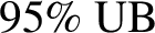
Safety (audit-level). Over the \(50\) stable audit cells we observe \(0/50\) anti-conservative violations at \(\gamma_\alpha{=}1.0\); the exact-binomial \(95\%\) upper bound for a zero-failure sample of size \(50\) is \(1-0.05^{1/50}=5.8\%\). Per-family bounds are wide for small \(n\) (the \(n{=}8\) subset alone gives a \(31.2\%\) upper bound), so the pooled set carries the strength; the breakdown is in Appendix A. As a supporting held-out diagnostic, the calibrated curve passes \(86/86\) one-sided coverage checks at the finer curve level — reported separately because curve-level checks within an audit are not independent and would inflate the effective sample size if treated as the primary denominator.
Sharpness (is it safe because useless?). No. As a point-level diagnostic over \(172\) cell\(\times\)tolerance checks, the certified-to-measured horizon ratio \(H^{\mathrm{conf}}/H^{\mathrm{meas}}\) has median \(0.67\), IQR \([0.38,1.0]\), with \(0/172\) anti-conservative; \(98\%\) of checks retain \(\ge 25\%\) of the measured horizon, \(69\%\) retain \(\ge 50\%\), and \(27\%\) are exactly tight (\(H^{\mathrm{conf}}{=}H^{\mathrm{meas}}\), including correctly certifying the full \(8\)-step horizon). The certificate is one-sided conservative and non-vacuous. Horizons are short integers (\(H\in[1,8]\), the neutral regime), so it is best read as a sharp short-horizon feasibility gate rather than a long-horizon point predictor.
![Figure 2: The certificate is one-sided conservative and non-vacuous. Left: certified vs. measured horizon over 172 audit checks — every point in the conservative region, with real spread (at H_{\mathrm{meas}}{=}8 the certified horizon ranges 1–8, including tight points). Right: the ratio H_{\mathrm{conf}}/H_{\mathrm{meas}} (median 0.67, IQR [0.38,1.0], 0/172 anti-conservative). Point-level diagnostic; the formal audit-level safety accounting remains the 50-cell table.](/article/2606.24946/figs/fig_sharpness.png "fig:")
0.13 5. Calibration Cost Across Substrates↩︎
Corollary C predicts that equivariance removes the orbit-wise calibration cost. We test this directly at the certificate level: place a held-out set at each of \(K\) orbit sectors (the group action on inputs and actions), audit each sector, then calibrate \(\gamma\) on \(m\) sectors and ask whether the certificate stays one-sided valid over the whole orbit (calibration and test sectors disjoint). This is a boundary test — it asks when the predicted structural saving becomes an empirical one — and the answer depends on the substrate.
0.14 5.1 Symmetric 2D: no separation↩︎
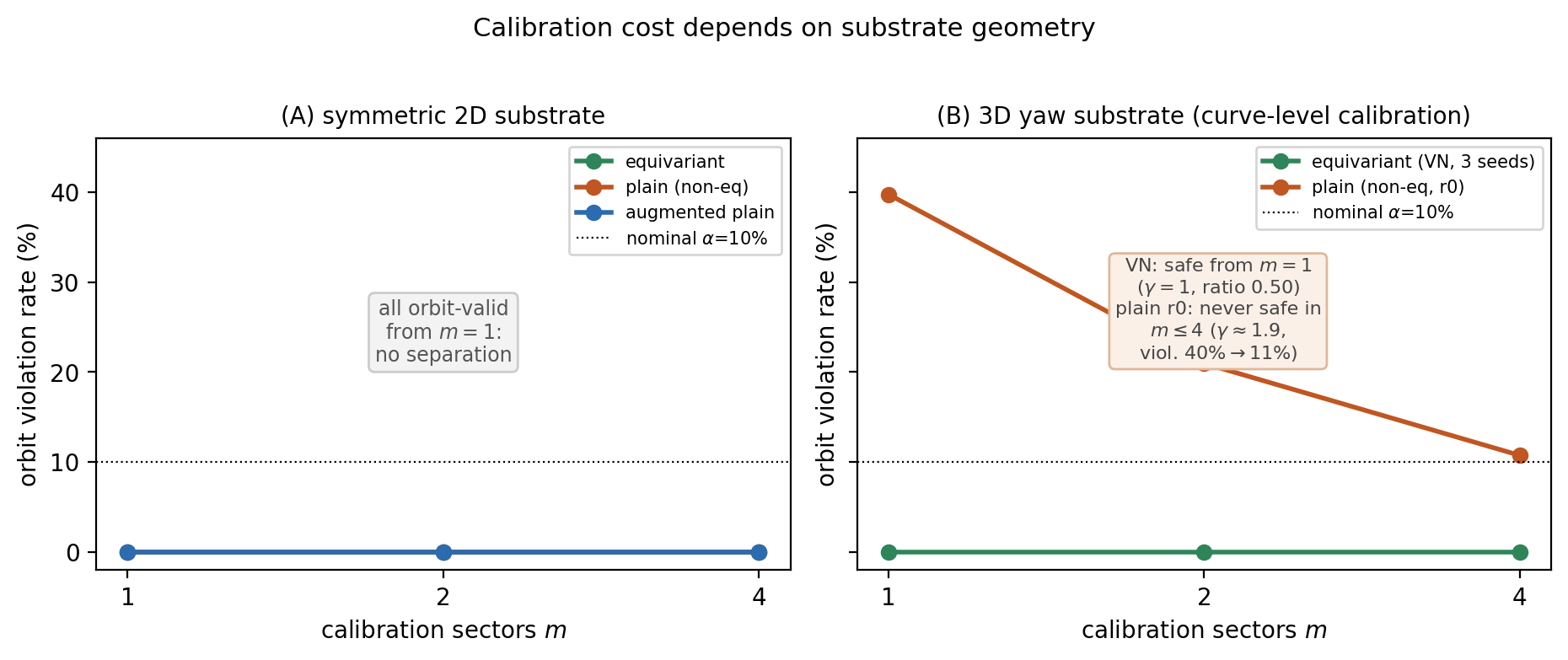
On the circular-masked 2D PushT substrate, equivariant, plain (non-equivariant), and R-augmented models all show \(0\%\) orbit anti-conservative violations from a single calibration sector (\(m{=}1\)); the orbit non-constancy of \(\hat{\delta}\) is small for all three (spread \(\le 8\%\)), and the augmented model is in fact the most orbit-robust (Fig. 3A). The theorem-side transport holds (Section 3.4), but this substrate does not expose a calibration-cost separation: a globally rotation-symmetric arena makes even non-equivariant CNNs approximately orbit-robust for free.
0.15 5.2 3D yaw: the separation appears↩︎
On a 3D point-cloud manipulation substrate audited under the gravity-preserving yaw subgroup (\(SO(2)\); full \(SO(3)\) is a representation-level symmetry but not a tabletop dynamics symmetry, Section 3.3), the plain baseline no longer receives orbit robustness for free. All multipliers and violation rates in this subsection use the curve-level score \(\Gamma_i\) of Proposition B (the deprecated horizon-division proxy is retained only as a sanity check; Appendix A.3). The equivariant Vector-Neuron model obtains a one-sector safe and non-vacuous certificate, consistently across \(3\) seeds: \(0\) anti-conservative violations at every \(m\), \(\gamma_\alpha{=}1.0\), median \(H^{\mathrm{conf}}/H^{\mathrm{meas}}=0.50\), utility-preserving coverage \(75\%\) at \(\tau{=}0.4\), and minimal calibration sectors \(m^*_{0.4}=1\) (Fig. 3B).
Healthy plain seeds do not obtain this certificate, and the cost takes different forms across seeds. Plain seed r0 does not reach orbit safety within the audited sector budget \(m\in\{1,2,4\}\): its violation rate falls from \(40\%\) to \(21\%\) to \(11\%\) but stays anti-conservative, even though it already pays a slack multiplier \(\gamma_\alpha\approx1.9\). The second healthy plain seed (r2) is conservative (\(0\) violations) but loses sharpness — median \(H^{\mathrm{conf}}/H^{\mathrm{meas}}\approx0.38\), below the \(\tau{=}0.4\) utility threshold. A third plain seed fails the pre-registered stability filter (latent collapse) and is reported separately (Appendix A). So the non-equivariant baseline does not obtain the one-sector safe-and-sharp certificate; the cost surfaces as violation, slack, sharpness collapse, or seed instability.
These residual plain violations are expected, not a breakdown of the conformal machinery: for a non-equivariant model the locally calibrated sector is not guaranteed exchangeable with the rest of the orbit, so a wedge-calibrated certificate carries no zero-shot transport (Corollary C needs the equivariance hypothesis). The remaining violations are precisely the empirical price of that missing structure. The 3D audit otherwise uses the same certificate definition as the rest of the paper: the GPU rollout implementation is verified equal to the canonical CPU audit on shared cells (\(\hat{\delta}\) \(4.6526\) vs \(4.653\); identical horizon cells; Appendix A).
0.16 5.3 Takeaway↩︎
The two substrates are complementary regimes. The orbit-transport theorem is structural and always holds; the empirical calibration-cost saving appears only when ordinary baselines do not already acquire orbit robustness from the data distribution. On the symmetric 2D arena they do, so the separation is null; on the 3D yaw substrate they do not, so equivariance yields a one-sector certificate that non-equivariant baselines cannot stably match. Calibration has geometry, but whether that geometry pays off empirically is a property of the substrate.
0.17 6. Scope and Boundaries↩︎
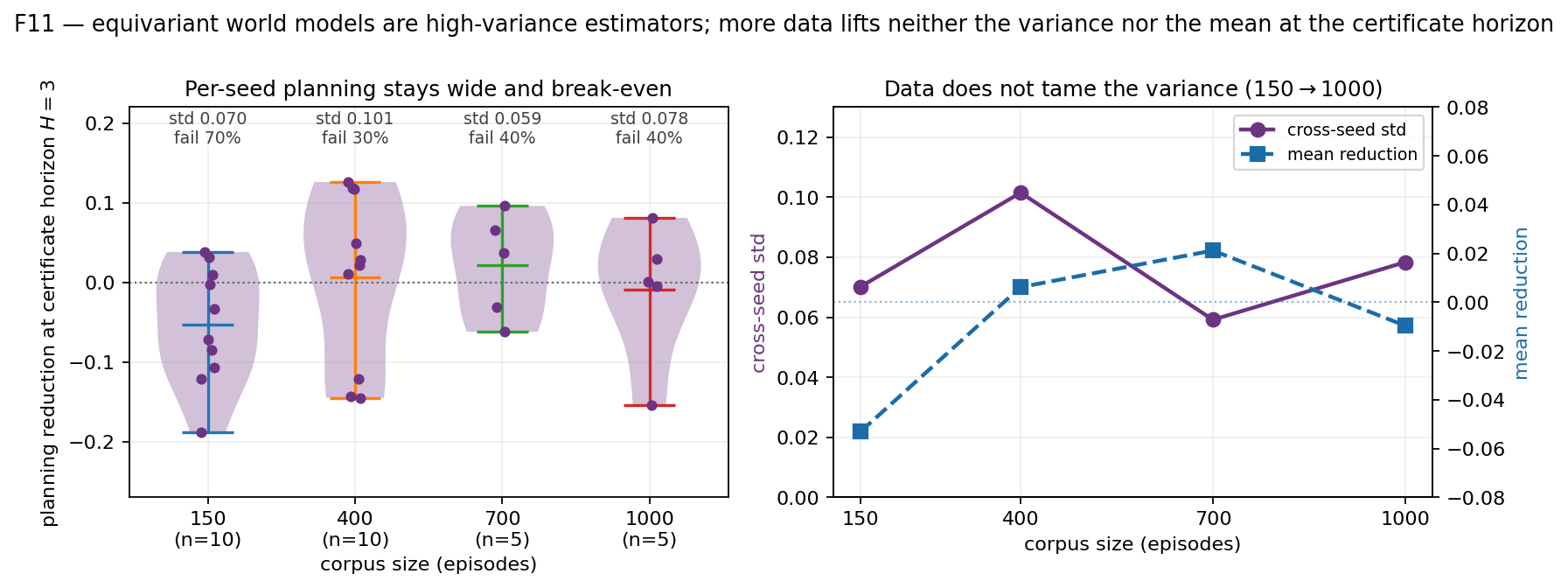
What else the structure buys and costs. Beyond the certificate, equivariance shows a low-data prediction edge that scale erases, a persistent readability/group-coordinate advantage, and a high-variance cost; on our 2D pixel substrate neither corpus size nor input resolution improved latent predictive precision. We characterize these in Appendix D. The binding finding there — equivariant world models are high-variance estimators — is the cost side that the planning non-confirmation below makes concrete.
The certified horizon \(H^*(\epsilon)\) is, by construction, a planning quantity: it states how far a hierarchical controller may space its subgoals before the model’s error exceeds tolerance. The natural application — certified subgoal spacing, replacing FF-JEPA’s fixed \(H{=}25\) with a data-derived, orbit-valid function — is also where structure must pay off as behavior. We report this attempt in full, including its negative result, because the boundary is itself the finding.
0.18 6.1 The substrate test↩︎
We built a from-scratch latent CEM-MPC planner that rolls the equivariant predictor \(f\) forward over a horizon \(H\), scores action sequences by the predicted read-out distance to the goal, and re-plans (3D point-cloud PickCube, reusing the paper’s machinery). The pre-registered, certificate-aware question was minimal: does latent CEM-MPC beat open-loop/random, and does \(H^*(\epsilon)\) predict the optimal \(H\)?
0.19 6.2 A single-seed signal that did not survive multiplicity↩︎
On the first seed the result was clean and certificate-consistent: blind planning at \(H{=}8\) drifted away from the goal, while gating the horizon to \(H{\approx}3\text{–}4\) — exactly where the predictor’s measured rollout error crosses the \(\epsilon{\approx}0.1\) tolerance (\(H^*(\epsilon)\)) — produced a positive, peaked reduction-vs-\(H\) curve that fell off as the horizon entered the untrustworthy region. Taken alone, this is an initial positive signal.
It did not replicate. Under the project’s discipline (\(n\ge10\) for weak effects), a well-powered sweep (\(n{=}10\) encoders at \(400\) episodes) shows the planning substrate is high-variance: \(3/10\) seeds fail at every horizon and the per-seed optimum spreads across \(H\in\{2,3,4,8\}\). A formal test finds no detectable trust-horizon / best-horizon association (\(\tau_b{=}-0.15\)), but it is underpowered, so this is no evidence of a link, not a demonstrated absence (Appendix C). The binding, well-powered finding is the variance: more data tames the bias but leaves the cross-seed std in \(0.06\)–\(0.10\) across \(150\to1000\) episodes (Section 4.3) — the single-seed signal was a seed-dependent effect. (A contact-rich variant, PushCube, behaved no differently, with \(7\text{–}13\%\) first non-zero success.) This is the cost side of the structure–variance economics (Section 4) made concrete.
Scoping the negative. This is not a claim that latent planning is infeasible: concurrent hierarchical latent planners reach \(\sim70\%\) on real-robot pick-and-place [2]. Our narrower negative: certificate-gated, single-level CEM-MPC on a high-variance equivariant substrate does not deliver. Whether certified spacing can be made to pay off remains open.
0.20 6.3 Diagnosis: a state-sufficiency hypothesis↩︎
The failure pattern has a precise structural reading. Our predictor’s action-response — how accurately \(f(z,a)\) moves the read-out end-effector in the direction the true end-effector moves — is the weak, high-variance component (cosine \(0.30\text{–}0.60\) across seeds), while the encoder’s static quality (latent norm, coordinate readability) is stable. A planner needs to predict dynamics; our latent carries only configuration. A direct symptom: an action-mismatch broken-equivariance control is uninformative here, because zeroing the action leaves the one-step residual unchanged (\(\hat{\delta}_{\text{zero-act}}=\hat{\delta}_{\text{real-act}}\)) — the predictor barely uses the action. (This is why Section 5 uses the non-equivariant checkpoint, not an action mismatch, as its representation-broken control.)
This is consistent with a state-sufficiency bottleneck (a hypothesis motivated by the failure mode, not a demonstrated cause): we impose symmetry on the configuration group \(SE(3)\), but a world model is a dynamics object, and a position-centric latent may under-determine the rollout — one cannot predict how an object moves from where it is without how fast it is going. A sharp asymmetry sharpens it: on a tabletop, gravity breaks the spatial rotation the architecture leans on (\(SO(3)\!\to\!SO(2)\)) yet preserves Galilean boost — the symmetry we never exploit.
Future work. We therefore leave certified planning to a phase-space-equivariant substrate (latent carrying velocity, predictor Galilean-/boost-equivariant), with a clean falsification: does adding the velocity state and boost equivariance reduce the planning variance and recover the certificate\(\to\)horizon link? — stated as a hypothesis, not a result.
0.21 7. Related Work and Positioning↩︎
Latent world models and hierarchical planning. We work in the latent-prediction regime [JEPA; [3]; [4]; [5]] rather than pixel generation, which we argue (Appendix D) is the limiting abstraction, in our setup, for a predictive model. The closest neighbor is FF-JEPA [1], hierarchical latent planning with an action-free subgoal predictor: it establishes the planning-layer demand but leaves the subgoal gap \(H{=}25\) an unprincipled hyperparameter. Our \(H^*(\epsilon)\) is the principled answer it lacks — one number for one distribution becomes a function valid over the orbit — which is also why our negative planning result (Section 6) does not collide with FF-JEPA: we share the demand, not a working planner. HWM [2] supplies a post-hoc error-vs-horizon analysis (its Fig. 6) that is the empirical shadow of our certified curve; the differentiator is a priori, orbit-transported derivation vs post-hoc measurement.
Equivariance, geometric deep learning, and generalization. The encoder builds on \(E(n)\)/steerable and Vector-Neuron equivariance [6]–[9], and equivariant RL and policies [10]–[12] share the shared-encoder pattern we reuse. The generalization benefit of equivariance is partly understood theoretically — a provably strict generalization gain on symmetric targets [13] — and empirically contested at scale [14]. That literature measures the benefit on a prediction loss; our claim is orthogonal to both architecture design and accuracy: Theorem A transports a calibrated certificate over the orbit, so a local audit becomes orbit-valid at no extra calibration cost — a statement about the certificate’s domain of validity, which prediction-generalization results do not address. Consistent with the project’s red-team discipline we do not claim “equivariance wins”: Appendix D shows the prediction edge is low-data (the Brehmer objection is correct on that axis) and Section 6 reports the planning negative in full.
Conformal prediction. Conformal prediction yields distribution-free, finite-sample validity under exchangeability [15], [16], with split-conformal and conformalized quantile regression as workhorses [17] and adaptive variants that relax exchangeability under distribution shift [18]; it has recently been applied to world-model verification [19]. We apply a one-sided multiplicative split-conformal calibrator to the entire trust-horizon curve (Section 3.2). What is new is the object, not the calibrator: prior work calibrates a scalar or an interval at a point, whereas we calibrate a horizon function and then transport that calibrated function over the group orbit (Theorem A) — a local audit becomes an orbit-valid certificate. A non-equivariant predictor can be conformalized too, but earns coverage only where it was calibrated; off that wedge it must collect fresh exchangeable data — a cost equivariance removes when the symmetry holds.
Reachability, barrier functions, and runtime assurance. Formal safety has a long control-theoretic tradition: Hamilton–Jacobi reachability computes backward-reachable sets for known dynamics [20], control barrier functions enforce forward-invariant safe sets [21], and runtime-assurance architectures switch to a verified fallback when a controller leaves its trusted envelope [22]. These certify a controller against a known or bounded model; our object is dual — how long a learned model can be trusted before rollout error breaks tolerance, with finite-sample conformal semantics rather than a worst-case reachable set. Such guarantees are stated per state or per trajectory; equivariance lets us state ours once per orbit, whereas a non-equivariant trust certificate must re-establish its smoothness budget across the orbit. The discrete-symmetry and companion neighbors are symmetry-protected neutral Lyapunov modes [23] and an audit line [24] that certifies off-the-shelf models at zero training cost.
0.22 Relation to the companion audit line↩︎
The certificate machinery — the Benettin \(\hat{\lambda}_1\) expansion estimate and the dual-boundary feasibility gates — is shared with the companion audit line [24] that certifies off-the-shelf models; we do not claim it as novel. What is distinct here is the conformal one-sided calibration of the horizon curve (Section 3.2), the orbit-transport theorem for the calibrated curve (Section 3.3), the measured structure–variance economics (Appendix D), and the honest downstream boundary (Section 6). We are explicit about what this is and is not: a certified-horizons + honest-economics paper, not a certified-spacing-wins paper (Section 8 states the defensible result and its over-reach boundary).
0.23 8. Conclusion↩︎
We introduced conformal orbit-valid trust horizons for equivariant world models. The certificate is one-sided and distributional: it is calibrated relative to the measured audit distribution, not a global reachability guarantee. The key structural result is that exact equivariance transports conformal validity over a group orbit, so the orbit-wide event is not a union over transformations but the same calibrated event viewed through the group action. Empirically the certificate is safe and non-vacuous: \(0/50\) audit-level anti-conservative violations, a \(95\%\) upper bound of \(5.8\%\), and median sharpness \(H_{\mathrm{conf}}/H_{\mathrm{meas}}=0.67\); implementation-level transport residuals are small (median \(1.1\%\)). At the same time, the symmetric 2D substrate is already orbit-robust for non-equivariant and augmented baselines, so the calibration-cost separation is mild rather than dramatic. The natural downstream use — certified subgoal spacing — remains a separate control-layer problem, not confirmed in our high-variance 3D planner. The main lesson is that equivariance does not replace calibration; it gives calibration a geometry.
0.24 A. Audit accounting and the reproducible set↩︎
We report results on the reproducible audit set rather than the looser candidate count. The set is defined by pre-specified stability/reproducibility filters applied before the anti-conservatism indicator \(V_i\) is evaluated, so the filtering cannot select for or against violations.
Figure 4: |
Figure 5: |
Figure 6: |

|
|---|---|---|---|
| Candidate records | all generated audit artifacts | No | |
| Reproducible | parseable certificate JSON, valid \(c_3\) curve | No | |
| Stable cells | stability criteria (no divergence, latent-std in range, logs present) | No | |
| \(V_i\) evaluated | \(V_i=\mathbf{1}\{H^{\mathrm{conf}}_i>H^{\mathrm{meas}}_i\}\) | Yes (post-filter) |
 .
.  .
.  .
. The \(75\to50\) reduction is not a removal of failed-outcome cells; it removes cells whose audit object is a-priori invalid (failed training, missing or unparseable artifacts). Filtered-out cases and their
reasons are listed in the artifact papers/tables/auditconformal.json.
0.24.1 A.1 Full per-family table↩︎
Figure 7: |
Figure 8: |
Figure 9: |
Figure 10: |
Figure 11: |
Figure 12: |
Figure 13: |
|
|---|---|---|---|---|---|---|---|
| Shape-OOD (CUDA) | /23 | % | |||||
| Champ (CUDA) | /10 | % | |||||
| Champ (MPS) | /8 | % | |||||
| Champ (MPS-cand) | /9 | % | |||||
| Total | 50 | 1.0 | 0/50 | 5.8% | |||
| Orbit-transp. resid. | % | %\(^\ddagger\) |
 .
.  .
.  .
.  .
.  .
.  .
.  .
. Families correspond to the recorded shape-OOD, champion (CUDA / MPS / MPS-cand), and wedge audit JSONs (stems in auditconformal.py). The small per-family bounds are deliberately reported: with \(n{=}8\) the
\(95\%\) upper bound is \(31.2\%\), so any single small family is weak evidence; the strength is the pooled \(n{=}50\) (\(5.8\%\)). Exact zero-failure binomial bound: \(1-0.05^{1/n}\). (\(^\ddagger\) the orbit-transport row reports median / max transport residual, not a
binomial bound.)
0.24.2 A.2 Conformal calibration details↩︎
The split-conformal multiplier is selected on a calibration split of audit \((\text{cell},\epsilon)\) pairs and evaluated on a disjoint test split. Consistent with the multiplicative curve calibration \(\widehat{\mathrm{Err}}^{\mathrm{conf}}=\gamma_\alpha\widehat{\mathrm{Err}}\) (Section 3.1), the nonconformity score is the minimal curve multiplier that makes the certified horizon conservative, \(\Gamma_i=\inf\{\gamma\ge 1: H^{\gamma}_i\le H^{\mathrm{meas}}_i\}\) with \(H^{\gamma}_i=\max\{H:\gamma\widehat{\mathrm{Err}}_i(H)\le\epsilon\}\), and \(\gamma_\alpha=Q_{1-\alpha}(\Gamma_{\mathrm{cal}})\), \(\alpha=0.1\). On the reproducible audit set every recorded \((\text{cell},\epsilon)\) already satisfies \(H^{\mathrm{raw}}_i\le H^{\mathrm{meas}}_i\) (the raw curve is one-sided conservative — equivalently the recorded horizon ratio \(H^{\mathrm{raw}}_i/H^{\mathrm{meas}}_i\le 1\)), so \(\Gamma_i=1\) throughout and \(\gamma_\alpha=1.0\): no extra slack is required under the audit protocol. (Where a violation occurs, \(\Gamma_i>1\) and the curve multiplier differs from the bare horizon ratio; the two coincide only in the all-conservative regime we record here.) This does not make calibration vacuous — it supplies the finite-sample coverage interpretation under exchangeability and prevents the raw median-\(\hat{\delta}\) curve from being presented as an uncalibrated guarantee.
Denominator note. Our primary statistical accounting is at the run/audit level: \(0/50\) anti-conservative audits, \(95\%\) upper bound \(5.8\%\). At the finer curve/checkpoint level the calibrated audit passes all \(86/86\) recorded one-sided coverage checks on the held-out split; we report this only as
supporting diagnostic evidence, because curve-level checks within an audit are not independent and would inflate the effective sample size if treated as the primary denominator. Reproduce both with papers/figures/auditconformal.py.
0.24.3 A.3 3D yaw audit: health filter, per-seed cost, and GPU/CPU equivalence↩︎
The Section 5 3D result audits frozen checkpoints under the gravity-preserving yaw subgroup \(SO(2)\) (no retrain, no simulation). It is run on a separate point-cloud substrate (Vector-Neuron DGCNN encoder for the equivariant family, PointNet for plain), so it inherits its own stability filter rather than the 2D accounting above. We trained three seeds per family and applied the same pre-registered collapse filter used throughout the project (latent norm in range, \(\hat{\delta}\) not degenerate) before auditing.
Figure 14: |
Figure 15: |

|
|---|---|---|
| r0 | \(20.65\) / \(4.63\) — healthy | \(38.60\) / \(5.92\) — healthy |
| r1 | \(19.50\) / \(5.06\) — healthy | \(2.68\) / \(0.004\) — collapsed (excluded) |
| r2 | \(17.82\) / \(5.27\) — healthy | \(9.83\) / \(1.08\) — healthy |
 .
.  .
. VN is \(3/3\) healthy; plain is \(2/3\) healthy (r1 fails the filter by latent collapse and is excluded before the certificate is evaluated, so the exclusion cannot select for or against the result). The per-seed firm-up (calibrate on \(m\) sectors, test on the disjoint rest, \(R{=}10\) sector selections, \(50\) episodes, four separation modes; curve-level \(\Gamma_i\) score) is:
Figure 16: |
Figure 17: |
Figure 18: |

|
|---|---|---|---|
| VN r0 | \(0\%\) / \(1.00\) / \(0.50\) / \(75\%\) | \(1\) | none |
| VN r1 | \(0\%\) / \(1.00\) / \(0.44\) / \(50\%\) | \(1\) | none |
| VN r2 | \(0\%\) / \(1.00\) / \(0.50\) / \(75\%\) | \(1\) | none |
| plain r0 | \(40\%\) / \(1.94\) / \(1.20\) / \(34\%\) | violation + slack (unsafe in \(m\le4\)) | |
| plain r2 | \(0\%\) / \(1.00\) / \(0.38\) / \(33\%\) | sharpness |
 .
.  .
.  .
. All three VN seeds obtain a one-sector (\(m^*_{0.4}=1\)), zero-violation, non-vacuous certificate; r1 is slightly less sharp (ratio \(0.44\)), so \(\tau{=}0.4\) is the utility threshold at which all three qualify. Neither healthy plain seed matches, with a seed-dependent failure mode. Under the curve-level multiplier, plain r0 stays anti-conservative across the audited budget — violation rate \(40\%\to21\%\to11\%\) over \(m\in\{1,2,4\}\) (monotone but never reaching \(0\), so \(m^*_{0.4}\) is undefined in range), despite a slack \(\gamma_\alpha\approx1.9\); plain r2 is conservative but loses sharpness (median ratio \(0.38<\tau\)). Seed-dependence is itself part of the finding: non-equivariant orbit calibration is unstable, whereas the equivariant certificate is consistent.
Curve-level multipliers (and the retired proxy). All 3D conformal multipliers and violation rates above and in Fig. 3 use the curve-level nonconformity score \(\Gamma_i\) of Proposition B, computed by
papers/figures/recomputegammacurve3d.py from each sector’s \((\hat{\delta},\hat{\lambda})\) curve. The certified curve uses the \(q90\) residual scale, which the per-sector
artifacts do not store directly; the recomputation therefore reconstructs it by solving for the \(q90\) scale that exactly reproduces the stored certified horizons, and we verify that every recorded \(H^{\mathrm{cert}}\) (all four \(\epsilon\) levels, all eight sectors, every checkpoint) is recovered bit-for-bit before any \(\Gamma_i\) is computed. This is a
reconstruction for theory–implementation consistency, not a re-fit of the 3D result: the audited horizons are inputs, not free parameters. An earlier horizon-ratio diagnostic (\(H^{\mathrm{cert}}/H^{\mathrm{meas}}\) with \(H^{\mathrm{cert}}/\gamma\)) is kept only as an implementation sanity check and is not used for any reported conformal claim. The
distinction is immaterial for fully conservative families, where every \(\Gamma_i=1\) (so \(\gamma_\alpha=1.0\) for VN, plain r2, and the entire 2D set), and matters only for plain r0 — the
one family with raw anti-conservative cells (\(20/32\)). The residual plain-r0 violations under a positive \(\gamma_\alpha\) are the expected cost of lacking zero-shot orbit transport (for a
non-equivariant model the wedge-calibrated sector is not exchangeable with the rest of the orbit), not a failure of the conformal procedure. The horizon-division proxy was optimistic here — it reported plain r0 reaching safety by \(m{=}4\), which the curve-level score does not.
Scope. This is a yaw (\(SO(2)\)) audit, not full \(SO(3)\) tabletop dynamics, and it is a distributional audit of frozen models, not a global reachability guarantee. It establishes that the calibration-cost separation predicted by Corollary C does appear on a substrate where baselines are not already orbit-robust — complementing, not overturning, the 2D null.
GPU/CPU equivalence. The 3D audit uses a batched GPU rollout for speed; we verified it computes the same certificate as the canonical CPU auditpair on a shared checkpoint (vnr0) and the same two episodes:
| quantity | CPU canonical | GPU batched |
|---|---|---|
| \(\hat{\delta}\) | \(4.653\) | \(4.6526\) |
| \(\hat{\lambda}_1\) | \(0.0662\) | \(0.0662\) |
| horizon cells | \((2,3,1),(4,8,2),(8,8,3),(16,8,7)\) | identical |
The \(\hat{\delta}\) difference (\(<10^{-3}\)) is floating-point reduction order; the horizon cells the certificate actually emits are bit-identical. Reproduce with
experiments/p43dcalibcost.py, experiments/p43dhealth.py, experiments/p43dbatchequiv.py, and the analysis in papers/figures/analyzecalibcost3d.py.
0.25 B. Proof of Theorem A (orbit transport)↩︎
Setup as in the main text: \(G\) acts by \(x\mapsto g\!\cdot\!x\), \(a\mapsto\sigma(g)a\), \(z\mapsto\rho(g)z\); the transition \(T\), encoder \(E\), and predictor \(f\) are equivariant, and \(\rho(g)\) is norm-preserving.
Proof. Induction on \(t\). Base case \(t=0\): by definition of the transformed initial condition, \(z_0^g=\rho(g)z_0\) and \(\hat{z}_0^g=\rho(g)\hat{z}_0\). Inductive step: assume \(z_t^g=\rho(g)z_t\) and \(\hat{z}_t^g=\rho(g)\hat{z}_t\). Using equivariance of \(T\) and \(f\) and \(a_t^g=\sigma(g)a_t\), \[z_{t+1}^g=T(z_t^g,a_t^g)=T(\rho(g)z_t,\sigma(g)a_t)=\rho(g)T(z_t,a_t)=\rho(g)z_{t+1},\] \[\hat{z}_{t+1}^g=f(\hat{z}_t^g,a_t^g)=f(\rho(g)\hat{z}_t,\sigma(g)a_t)=\rho(g)f(\hat{z}_t,a_t)=\rho(g)\hat{z}_{t+1}.\] By the norm-preserving metric, \[\lVert\hat{z}_{t+1}^g-z_{t+1}^g\rVert=\lVert\rho(g)(\hat{z}_{t+1}-z_{t+1})\rVert=\lVert\hat{z}_{t+1}-z_{t+1}\rVert.\] The per-step error is orbit-invariant for all \(t\le H\); since \(\hat{\delta}\), \(\hat{\lambda}\), and the measured rollout error are functions of these per-step errors, they are orbit-constant, hence so is the raw curve \(\widehat{\mathrm{Err}}(H)=\hat{\delta}\sum_{t<H}e^{\hat{\lambda} t}\). Because \(\gamma_\alpha\) is a single scalar fixed on the calibration set (not orbit-dependent), \(H^{\mathrm{meas}}\) and \(H^{\gamma}=\max\{H:\gamma\widehat{\mathrm{Err}}(H)\le\epsilon\}\) for every fixed \(\gamma\ge 1\) — in particular \(H^{\mathrm{raw}}=H^{1}\) and \(H^{\mathrm{conf}}=H^{\gamma_\alpha}\) — are orbit-constant. Note this is constancy of each horizon as a functional of the orbit-constant curve; we do not claim the non-identity \(H^{\mathrm{conf}}=H^{\mathrm{raw}}/\gamma_\alpha\), which fails because \(\widehat{\mathrm{Err}}\) is nonlinear in \(H\). \(\blacksquare\)
Exact vs. approximate. The theorem is exact under exact equivariance. The implemented models are only approximately equivariant (finite training; quantized fibers), so we measure the transport residual \(\bigl|\,\lVert\hat{z}^g_t-z^g_t\rVert-\lVert\hat{z}_t-z_t\rVert\,\bigr|\) (the quantity Prop. D bounds) — median \(1.1\%\), max \(4.1\%\) over \(14\) audits — quantifying how closely the implementation realizes the theorem’s assumptions. We distinguish this from the out-of-wedge degradation (orbit non-constancy of \(\hat{\delta}\) without transport), median \(2.2\%\) / max \(6.0\%\) over the same audits: a related but looser diagnostic that does not isolate the equivariance defect.

0.26 C. Planning non-confirmation diagnostics↩︎
The 3D CEM-MPC non-confirmation (Section 6) rests on the well-powered variance finding, not the correlation test. For completeness: across \(n{=}10\) encoders at \(400\) episodes the
per-seed optimal horizon spreads over \(H\in\{2,3,4,8\}\) with \(3/10\) failing at every \(H\); the formal trust-horizon / best-horizon association is
Kendall \(\tau_b=-0.15\) (permutation \(p=0.60\)), which is underpowered (simulated power \(<0.4\) for \(\rho\le0.6\) at
\(n{=}10\)) and therefore reported as no evidence of a link, not a demonstrated absence. The cross-seed standard deviation stays in \(0.06\)–\(0.10\) across \(150\to1000\) episodes — data tames the bias, not the variance. Reproduce with papers/figures/hstarcorr.py.
0.27 D. Structure–variance economics and the price of pixels↩︎
These supporting characterizations motivate the Section 6 scope; they are not the paper’s headline and are demoted here from the main text.
Structure–variance economics. What equivariance buys, and whether scale erases it, measured as curves rather than a single benchmark point. (i) Prediction accuracy — a low-data edge: the one-step ratio \(\hat{\delta}_{\mathrm{plain}}/\hat{\delta}_{\mathrm{eq}}\) is \(2.4\)–\(3.3\times\) at \(\le 500\) episodes and closes by \(\sim 1000\) (a measured crossover; the scale objection of Brehmer et al. (2024) is correct on this axis). (ii) Readability and certificate — persistent: the group coordinate is decodable only from the equivariant latent (\(\theta\)-\(R^2\) \(0.91\) vs \(0.29\) at \(40\)k; 3D TCP-\(R^2\) likewise), and does not collapse with data — exactly where the prediction edge does. (iii) The cost — high variance: equivariant world models are high-variance estimators (cross-seed \(\hat{\delta}\) spread; e2cnn-on-MPS non-reproducibility; planner success swinging across seeds). The variance, not the bias, is the binding constraint downstream — the link to the Section 6 planning non-confirmation.
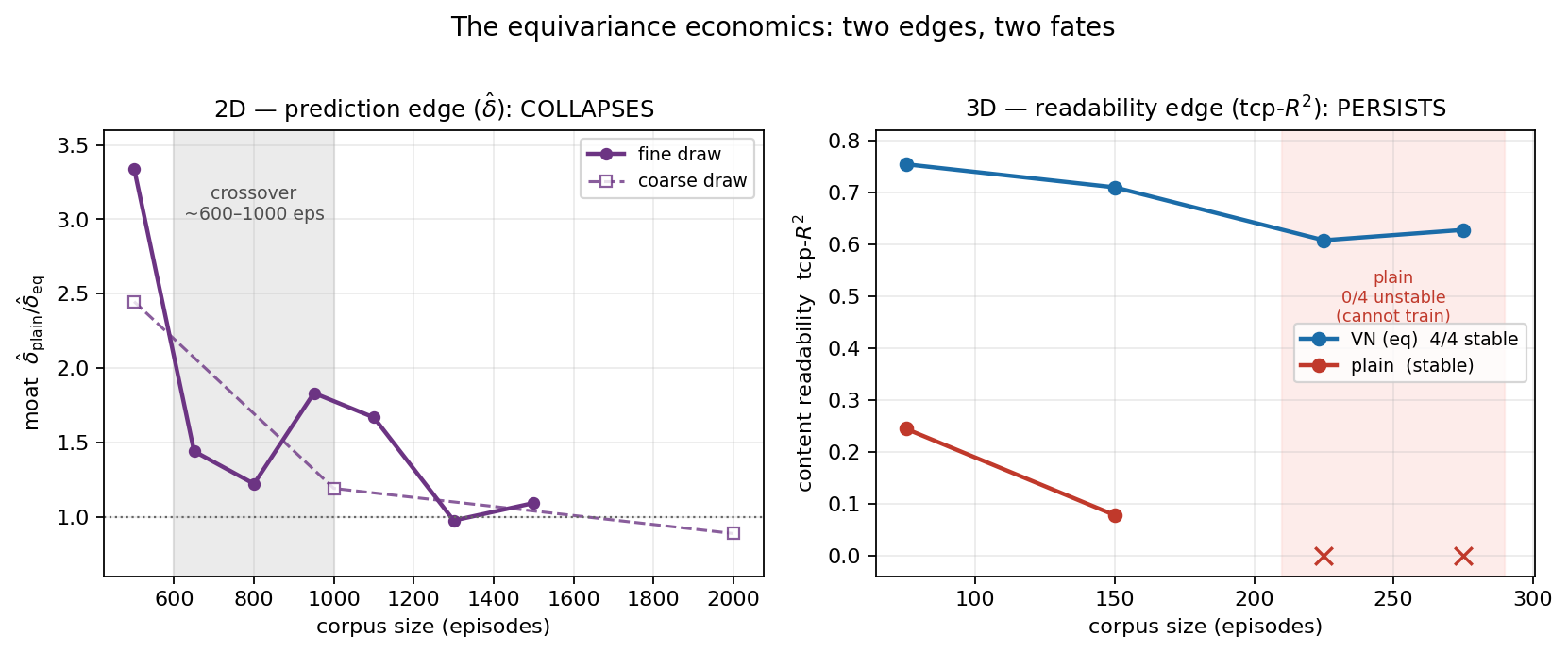
The price of pixels (under this substrate). Neither lever improved the latent’s predictive precision: \(\hat{\delta}\) is flat across corpus sizes \(c500\)–\(c2000\) on PushT pixels, and the resolution lever backfires — the unit-safe within-rung ratio \(\epsilon_{\mathrm{task}}/\hat{\delta}\) moves away from the GO regime at \(192\)px, where \(\hat{\delta}\) doubles (\(5.1\)–\(6.7\) vs \(1.6\)–\(3.3\)) while \(\epsilon_{\mathrm{task}}\) stays flat (NO-GO on all \(12\) cells; stage-A health passed \(4/4\), so the hit is on predictive precision, not stability). Under this substrate, architecture class, and sweep, the limiting factor is latent predictive precision, not sensor resolution — an empirical finding under the tested regime, not a universal claim about pixel-level modeling.