Large-Language-Model Discovery of Quantum LDPC Codes through Structured Concept Evolution
January 01, 1970
Abstract
Quantum computers could outperform classical machines on important problems, but only if the errors that pervade quantum hardware can be corrected at scale. Quantum low-density parity-check (qLDPC) codes offer a promising route to this goal by combining sparse parity checks with finite encoding rate and growing distance, but their construction remains a challenging discrete design problem. Here we introduce structured concept evolution (SCE), a search framework that pairs a large language model with a structured algebraic mutation grammar to discover lifted-product code families, a class of CSS qLDPC codes. Instead of asking the LLM to design codes from first principles, SCE evolves structured concepts consisting of algebraic specifications paired with executable programs that realize them, using hierarchical mutations that modify the group algebra, protograph geometry, or base space. Running SCE, we discover a diverse set of competitive code families, ranging from abelian constructions to families over non-abelian groups beyond those underlying standard designs such as bivariate-bicycle codes, and characterize them under code-capacity depolarizing noise with BP+OSD decoding. These results are obtained with lightweight models (GPT-5.4-mini and GPT-5.4-nano).
Quantum computers promise computational advantages for problems ranging from quantum simulation [1] and chemistry [2] to optimization and machine learning [3]–[7], but realizing them at scale requires quantum error correction, which encodes logical information redundantly into many physical qubits and repeatedly extracts syndromes from local parity checks [8]–[11]. The surface code has been the workhorse of this program owing to its planar geometry and high threshold [12]–[14], and recent experiments demonstrate repeated error correction and logical-error suppression on superconducting processors [15]–[17]. Yet it encodes a single logical qubit in \(\Theta(d^2)\) physical qubits, a vanishing rate shared by every two-dimensional geometrically local code [18], so its overhead remains the central obstacle to scaling. This obstacle is now practical rather than asymptotic: neutral-atom [19] and trapped-ion [20] platforms have reached or approached the thousand-qubit regime, so the number of logical qubits on a device is set directly by the rate of the underlying code. Constant-rate codes enable fault-tolerant computation with constant overhead [21]. At the error rates and code sizes relevant to near-term hardware they reduce the cost per logical qubit by roughly an order of magnitude relative to the surface code [22]. Demonstrations on reconfigurable atom arrays [23] and superconducting hardware [24], together with full architectural proposals for neutral-atom platforms [25], [26], make such codes concrete architectural targets. This motivates the search for quantum low-density parity-check (qLDPC) codes, which combine sparse parity checks with finite encoding rate and growing distance [27]–[31].
The central difficulty is that high-performing qLDPC codes are hard to find. The known families are built from algebraic product constructions: hypergraph product [27], generalized bicycle and related quasi-cyclic codes [32], [33], including the bivariate-bicycle (BB) codes [22] that descend directly from them, lifted product [28], [34], balanced product [35], fiber-bundle codes [36], quantum Tanner codes and other asymptotically good constructions [29], [31], [37], each parametrized by a small set of group-algebra elements or protograph polynomials. While these frameworks guarantee the CSS commutation structure [38], [39] by construction, the resulting performance depends on the specific group-algebra elements chosen, in a way that admits no closed-form optimum [40]. The viable region is a vanishingly small subset of an exponentially large discrete search space, and locating it has so far relied largely on expert intuition, exhaustive enumeration over small instances, or random sampling.
Machine-learning approaches have begun to address this as a combinatorial design problem. Reinforcement learning has been used to discover error-correction strategies, adapt codes to hardware-specific noise, and co-optimize stabilizer codes with their encoding circuits [41]–[43], as well as to scale automated circuit discovery [44] and reduce stabilizer measurement weight [45], but these methods search over explicit, finite-size stabilizer or circuit representations and do not yield the structured, scalable code families required at large block length. Here we take a different route, drawing on recent advances in large language models (LLMs). In the quantum domain, LLMs have been used for scientific exploration and experiment design [46], [47], and within multi-agent workflows for constructing nonadditive codes with prescribed transversal diagonal gates [48]. More recently, LLM-guided evolutionary search, with the LLM acting as an intelligent mutation operator [49], has emerged as a powerful tool for open-ended mathematical and algorithmic discovery, as demonstrated in FunSearch [50] and AlphaEvolve [51]. The qLDPC construction problem fits this paradigm well: a candidate code is cheap to specify and exactly verifiable, whereas the map from construction to performance is highly nontrivial.
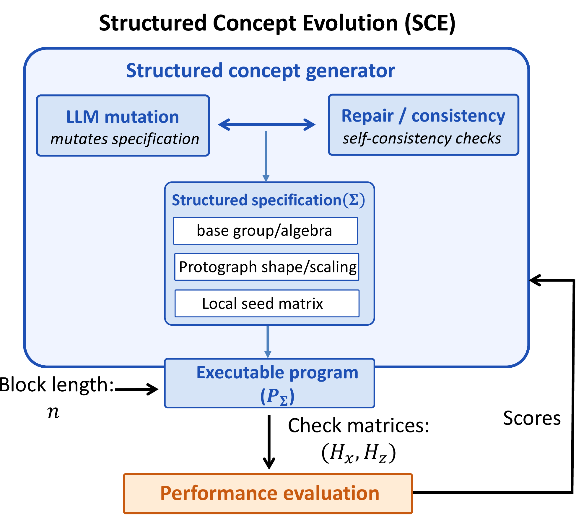
In this work, we introduce structured concept evolution (SCE), an evolutionary framework for the discovery of quantum LDPC codes. The evolving individuals are not codes but the higher-level concepts that generate them, where each such concept pairs a structured concept specification \(\Sigma\) with an executable program \(\mathsf P_\Sigma\) that generates the parity-check matrices of a CSS code at any admissible block length, as shown in Fig. 1. A large language model serves as the mutation operator, proposing edits at the level of these concepts. Applying SCE, we build a quality-diversity archive [52]. Instead of converging to a single optimized code, the archive retains many individually competitive constructions that differ across base group family, encoding rate, and decoding performance. We then benchmark the high-performing archive members under code-capacity depolarizing noise using Belief Propagation with Ordered Statistics Decoding (BP+OSD) [40]. We implement SCE on top of OpenEvolve [53], an open-source realization of AlphaEvolve.
General recipes.— Our search space consists of lifted-product (LP) CSS codes [28], [34], a general algebraic construction that generalizes the hypergraph product (HGP) and yields some of the most powerful modern qLDPC codes, including the first asymptotically good families [29]. LP codes are built from two base protographs, the analogues of the two classical HGP codes, given by matrices \(A\) and \(B\) of sizes \(m_A\times n_A\) and \(m_B\times n_B\) whose entries lie in the group algebra \(\mathbb{F}_2[G]\) of a finite group \(G\) of order \(q = |G|\). The lifted-product check matrices are obtained by applying the hypergraph-product rule at the protograph level and then replacing each group-algebra entry by its left or right regular representation [28]. Equivalently, with \(\widetilde{A}\) and \(\widetilde{B}\) denoting the corresponding block matrices, the CSS checks are \[\begin{align} H_X&=[\,\widetilde{A}\otimes I_{n_B}\mid I_{m_A}\otimes\widetilde{B}^{T}\,],\nonumber\\ H_Z&=[\,I_{n_A}\otimes\widetilde{B}\mid \widetilde{A}^{T}\otimes I_{m_B}\,] \label{eq:lp} \end{align}\tag{1}\] Because left- and right-multiplication commute, this satisfies \(H_XH_Z^{T}=0\) for any finite group \(G\). The code has \(n=fq\) physical qubits with \(f=n_An_B+m_Am_B\), so the block length scales linearly with the group order \(q\) (see Supplemental Material for details [54]).
The three mutation levels span a hierarchy from the broadest change to the most local. An algebraic (level-3) move replaces the base group family. Since the protograph shape, scaling rule, and local entries all depend on \(G\), they are rewritten as needed to remain valid for the new group. A shape/scaling (level-2) move keeps the group family fixed but changes the protograph dimensions \(m_A\times n_A\) and \(m_B\times n_B\), and hence we define \(f = m_Am_B+n_An_B\) and the block length \(n=fq\). A local (level-1) move keeps both \(G\) and the protograph shape fixed and only re-seeds the group-algebra entries of \(A\) and \(B\), leaving \(n\) unchanged. Because each move rewrites a structured construction rather than editing raw matrix entries, mutations move coherently between code families instead of isolated matrices. This structured grammar confers two practical advantages. It makes the search controllable, since the mutation-level distribution determines whether the search favors local refinement or broader algebraic exploration. It also makes the search interpretable, since each parent-to-child transition corresponds to a concrete construction-level operation, such as changing the base group, modifying the protograph, or re-seeding the local entries. Each iteration samples a parent scheme from the quality-diversity archive, assigns a mutation level uniformly at random (each of the three levels with probability \(1/3\)), and prompts the LLM with the parent scheme together with representative high-scoring archive entries as in-context examples. The LLM returns a complete child including specification and executable programs together (see Supplemental Material [54]).
![Figure 2: Hierarchical mutation and score evolution. (a) The three mutation levels, each shown as a representative parent \to child step drawn from the search log, with the resulting change in score and code parameters [[n,k]]. Level 1: the group and protograph shape are fixed and only the local \mathbb{F}_2[G] entries of the base matrices A and B are rewritten. Here we present the base matrix A. We consider the code based on \mathrm{Dic}_m, where r is the rotation generator (the order-2m cyclic element) and s is an order-4 element satisfying s^2=r^m and srs^{-1} = r^{-1}. Level 2: the group family is fixed as \mathrm{Dic}_m and the protograph shape changes, A,B:3\times4\to5\times3. At n\approx1500, the family parameter m shrinks 15\to11. Level 3: the base group transitions from the direct-product abelian group family \mathbb{Z}_2\times \mathbb{Z}_2\times \mathbb{Z}_{t} to the semidirect-product non-abelian group (\mathbb{Z}_2\times \mathbb{Z}_2)\rtimes \mathbb{Z}_{t}. (b) Program score of every evaluated candidate versus search iteration across the three 1000-iteration rounds. Dashed step curves trace the best score within each round. At the end of each round, the top-10 candidates with the lowest logical error rate at p=0.06 are seeded into the next round.](/article/2606.24808/mutation_and_evolution.png "fig:")
Because mutations act on an existing algebraic specification, the search proceeds at the level of structured concepts. For a faithful implementation of the lifted-product template in Eq. 1 , CSS commutation follows by
construction. This constrained search space makes the mutation task compatible with lightweight models. In our experiments, we use OpenAI’s GPT-5.4-mini for 40% of mutation calls and GPT-5.4-nano for the remaining 60%. The child program is executed to emit
\((H_X,H_Z)\) for any choice of \(n\). We scale the block size \(n\) within \(n_{\min}\le n\le n_{\max}\), with \(n_{\min}=600\) and \(n_{\max}=1500\), where we reject any candidate size that encodes no logical qubits or has a stabilizer weight exceeding a hard cap (here we take it as \(14\)), and we verify the CSS condition \(H_X H_Z^{\mathsf T}=0\) for every candidate. The surviving codes with the largest \(k\) are decoded with BP+OSD [28], [40], [55], as implemented in the ldpc package [40], under code-capacity depolarizing noise. We
evaluate for a small representative set of physical error rates \(\mathcal{P}=\{0.05,0.06,0.07\}\), where \(p\in \mathcal{P}\), yielding Monte-Carlo logical error-rate estimates \(\widehat p_L(p)\). For depolarizing noise the \(X\)- and \(Z\)-type errors are decoded independently. During the search, belief propagation uses the min-sum
update rule [56] with a BP iteration limit of \(2000\), followed by order-\(1\) combination-sweep ordered-statistics post-processing [40], and each \(\widehat
p_L(p)\) is estimated from \(2000\) random depolarizing error samples. When no failure is observed, the zero estimate is replaced by \(\widehat p_L=2.5\times10^{-4}\) (half a failure
in the \(2000\)-sample). We summarize the protection at each \(p\) by a pointwise effective suppression exponent \(\alpha(p)=\ln(1/\widehat p_L)/\ln(1/p)\)
and define the fitness score: \[\mathcal{S}=\frac{\gamma k}{n_{\max} |\mathcal{P}|}\,
\sum_{p\in\mathcal{P}}\alpha(p)^2 .
\label{eq:score}\tag{2}\] Here \(\alpha(p)\) scores how strongly a code suppresses errors at a single rate \(p\), which is evaluated pointwise. The score is used for selection
and does not certify code distance. The factor \(\gamma\) is a Tanner-graph novelty factor that penalizes candidates whose graph fingerprints are close to those already stored in the archive, thereby discouraging
rediscovery of near-duplicate constructions. Selected candidates populate an island-structured population, maintained with a per-island MAP-Elites [52] whose axes record the code rate \(k/n\), the decoder success score, and inherited seed-lineage label according to their base group family. The specification grammar, mutation and repair
operators, archive parameters, and novelty weighting are detailed in the Supplemental Material [54].
Discovered codes.— The search is seeded with lifted-product CSS codes spanning both abelian and non-abelian base groups listed in Table 2. We then run SCE for three sequential rounds of \(1000\) iterations each. Within a round, each iteration applies a single mutation whose level is drawn independently and uniformly from \(\{1,2,3\}\) with probability \(1/3\) for each level. At the end of each round, the \(10\) candidates with the lowest logical error rates at \(p=0.06\) are used as the seed programs in the next round. We note that selecting these seeds by logical error rate steers the evolution toward codes with better decoding performance. After three rounds, the search has generated \(3000\) candidate constructions. Each admitted child is executed to produce \((H_X,H_Z)\) and evaluated under a code-capacity depolarizing noise model using BP+OSD [Eq. 2 ].
Figure 2 (a) shows a representative parent\(\to\)child example at each level. In this example, at Level 1, only the exponents of the \(A,B\) entries are modified while the group and protograph shape remain unchanged. At Level 2, the protograph shape is reshaped from \((3\times 4, 3\times 4)\) to \((5\times 3, 5\times 3)\), and the entries of the protograph are also changed accordingly. At the highest level of the hierarchy, Level 3, the abelian direct-product group \(\mathbb{Z}_2\times \mathbb{Z}_2\times \mathbb{Z}_{11}\) is transformed into the non-abelian semidirect-product group \((\mathbb{Z}_2\times \mathbb{Z}_2)\rtimes \mathbb{Z}_{10}\). The protographs of these parent-to-child examples are listed in Supplemental Material [54]. Figure 2 (b) shows the program score across the three concatenated rounds. The running-best score improves from \(0.17\) to \(0.62\). The mutations across levels contribute unequally: level-1 mutations preserve the block length \(n\) and make only local adjustments to the entries, whereas level-2 and level-3 mutations restructure the protograph or replace the base group family, changing valid code block length and enabling larger jumps in the code-parameter landscape.
| Source | Base group | Abel | \([[n,k,d]]\) | \(kd^2/n\) |
|---|---|---|---|---|
| R1Elite01 | \(\mathbb{Z}_{3} \times\mathbb{Z}_{14}\) | ✔ | \([[1428,186,\le 18]]\) | \(\le 42.2\) |
| R1Elite02 | \(\mathbb{Z}_2\times\mathbb{Z}_2\times \mathbb{Z}_{11}\) | ✔ | \([[1496,198,\le 16]]\) | \(\le 33.9\) |
| R2Elite01 | \(\mathrm{Dic}_{11}\) | \(\times\) | \([[1496,194,\le 20]]\) | \(\le 51.9\) |
| R2Elite02 | \(\mathrm{D}_{22}\) | \(\times\) | \([[1496,198,\le 16]]\) | \(\le 33.9\) |
| R3Elite01 | \(\mathrm{Dic}_{11}\) | \(\times\) | \([[1496,192,\le 16]]\) | \(\le 32.9\) |
| R3Elite02 | \(\mathrm{Dic}_{11}\) | \(\times\) | \([[1496,198,\le 14]]\) | \(\le 25.9\) |
Table 1 lists representative high-scoring codes from each round. At \(n\approx1500\), the discovered families reach high encoding rate (up to \(k/n\simeq0.13\)). Finite-length non-abelian LP codes have so far been explored mainly through exhaustive enumeration of two-block ansatz codes at small block lengths [58]. SCE instead reaches them by open-ended search over arbitrary protograph shapes at \(n\approx1500\). Exact minimum-distance computation is NP-hard for general linear codes [59], so the distances of discovered codes in Table 1 are upper bounds computed with the QDistRnd GAP package [57], which searches for low-weight logical operators by random information-set decoding over \(10^5\) trials. Using the QDistRnd-found distance as an empirical distance proxy, the best discovered codes reach \(k d^2/n\) values up to about \(51.9\).
![Figure 3: Performance of evolved LP codes against BB baselines under code-capacity depolarizing noise. The logical error rate is reported per logical qubit, \epsilon_L = 1-(1- p_L)^{1/k}. (a) Encoding rate k/n versus \epsilon_L at fixed physical error rate p=0.06 for the top two LP elites of each set (blue: \mathcal{C}_{p_L}, green: \mathcal{C}_{\mathrm{score}}) and four BB codes (red). ^\dagger denotes an upper bound on the distance. Points toward the upper-left are preferable (high rate, low logical error). The \mathcal{C}_{\mathrm{score}} set attains the highest rate k/n\!\approx\!0.13 among all codes shown. (b) \epsilon_L versus p for the top two LP codes of each set and the four BB codes. Markers match panel (a). Error bars are 95% Clopper–Pearson confidence intervals [60].](/article/2606.24808/rate_and_waterfall.png "fig:")
Performance under depolarizing noise.— We characterize selected codes under code-capacity depolarizing noise with \(10^6\) sampled errors per point, decoded by the same BP+OSD scheme as in the search but at
heavier settings: a BP iteration limit of \(5000\) and order-\(4\) combination-sweep OSD. For this study, we select two sets of discovered codes from the third round. The first set, \(\mathcal{C}_{\mathrm{score}}\), consists of the two codes with the highest fitness scores, R3Elite01 and R3Elite02, listed in Table 1. The second set \(\mathcal{C}_{p_L}\) consists of the two codes with the lowest logical error rate at physical error rate \(p=0.06\), namely R3EliteP01 and R3EliteP02. These two elite
codes are based on the non-cyclic abelian group \(\mathbb{Z}_{30}\!\times\!\mathbb{Z}_2\) with the code parameters \([[1500, 81, \leq 18]]\) and \([[1500,76,\leq
20]]\), respectively. Although \(\mathbb{Z}_{t}\!\times\!\mathbb{Z}_2\) was not among the seed programs, it emerged during the SCE search. As a reference, we also include BB codes with block lengths \(144\)–\(756\). Figure 3 (a) shows the encoding rate \(k/n\) versus the logical error rate per logical qubit \(\epsilon_L = 1-(1- p_L)^{1/k}\) at fixed \(p=0.06\), where \(p_L\) is the block logical error rate. The \(\mathcal{C}_{\mathrm{score}}\) set reaches \(k/n\!\approx\!0.13\), while \(\epsilon_L\) at this point (\(\sim\!10^{-5}\)) is
lower than that of three of the four BB references (\([[144,12,12]]\), \([[288,12,18]]\), and \([[360,12,\leq24]]\)). Figure 3 (b) shows the full \(\epsilon_L\) versus \(p\) waterfall curves for the top two codes of each discovered set, together with the same BB codes. Every curve
exhibits the expected error-suppression behavior as \(p\) decreases. \(\epsilon_L\) for the discovered codes (\(\mathcal{C}_{p_L}\) codes \([[1500,81, \leq 18]]\) and \([[1500,76, \leq 20]]\)) is comparable to or below the baseline \([[756,16, \leq34]]\), over the measured range, while encoding
roughly five times as many logical qubits.
Conclusion.— We introduced structured concept evolution, an LLM-guided search over qLDPC construction schemes. Applied to lifted-product codes, SCE builds a quality-diversity archive of competitive constructions at \(n\approx1500\) that trade encoding rate against logical-error suppression. The search yields competitive constructions across both abelian and non-abelian groups, reaching non-abelian families beyond those underlying bivariate-bicycle designs. All results are obtained with lightweight models (GPT-5.4-mini and GPT-5.4-nano).
Several directions follow naturally. First, encoding a target platform’s qubit-connectivity graph into the mutation grammar or fitness score would steer the search toward hardware compatible codes. Since connectivity governs syndrome extraction depth, this also couples the search to a circuit-level objective. Second, SCE is not tied to lifted products. The same method can broaden to the balanced product, quantum Tanner codes, and fiber-bundle codes. It is also an open question whether SCE could propose entirely new CSS preserving constructions. Finally, one could co-design the code together with its encoding circuit and decoder, turning SCE into an end-to-end search over code, encoder, and decoder.
Note added.— During the preparation of this manuscript, a preprint appeared [61], also introducing LLM-based methods for the discovery of BB codes, whereas we explore the broader class of lifted-product codes.
Acknowledgments.— This research is part of the Munich Quantum Valley, which is supported by the Bavarian state government with funds from the Hightech Agenda Bayern Plus.
Supplemental Material for:
Large-Language-Model Discovery of Quantum LDPC Codes
through Structured Concept Evolution
S1. Lifted-product construction and CSS validity↩︎
0.0.0.1 Calderbank–Shor–Steane (CSS) codes.
A CSS code [38], [39] is specified by two binary parity-check matrices \(H_X\) and \(H_Z\) with the same number of columns (number of physical qubits). The rows of \(H_X\) define \(X\)-type stabilizers, and the rows of \(H_Z\) define \(Z\)-type stabilizers. The two sets of stabilizers commute if and only if \[H_X H_Z^{\mathsf T}=0 \pmod 2 . \label{eq:css}\tag{3}\] If the matrices have \(n\) columns, then the code has block length \(n\) and encodes \[k=n-\operatorname{rank}_2 H_X-\operatorname{rank}_2 H_Z\] logical qubits. Thus, a central task in constructing CSS codes is to generate parity-check matrices for which Eq. 3 holds.
0.0.0.2 Hypergraph product (HGP) codes.
Let \[A\in\mathbb{F}_2^{m_A\times n_A}, \qquad B\in\mathbb{F}_2^{m_B\times n_B}\] be two classical binary parity-check matrices. The hypergraph product defines [27] \[\begin{align} H_X &= \bigl[\,A\otimes I_{n_B} \;\big|\; I_{m_A}\otimes B^{\mathsf T}\,\bigr], \nonumber\\ H_Z &= \bigl[\,I_{n_A}\otimes B \;\big|\; A^{\mathsf T}\otimes I_{m_B}\,\bigr]. \label{eq:hgp} \end{align}\tag{4}\] Then \(H_XH_Z^{\mathsf T}\) contains two identical contributions, \(A\otimes B^{\mathsf T}+A\otimes B^{\mathsf T}\), which cancel over \(\mathbb{F}_2\). Hence \(H_XH_Z^{\mathsf T}=0\). In other words, the CSS condition follows from the two-sector structure of Eq. 4 .
0.0.0.3 Lifted-product codes.
Lifted-product codes preserve the same mechanism as HGP: the product \(H_XH_Z^{\mathsf T}\) again decomposes into two matching contributions that cancel over \(\mathbb{F}_2\), while the scalar entries of \(A\) and \(B\) are replaced by structured permutation blocks.
Let \[A\in \mathbb{F}_2[G]^{m_A\times n_A},\qquad B\in \mathbb{F}_2[G]^{m_B\times n_B}\] be two small matrices over the group algebra of a finite group \(G\) of order \(q = |G|\). An entry of \(A\) (and likewise \(B\)) is a formal sparse sum \(a=\sum_{g\in G} a_g g\) with the coefficient \(a_g\in\mathbb{F}_2\). To obtain ordinary binary matrices, each such group element is replaced by a \(q\times q\) permutation block sum. More explicitly, we use the left regular representation for entries of \(A\) and the right regular representation for entries of \(B\), \[a\mapsto \lambda(a)=\sum_{g\in G} a_g\,\lambda(g),\qquad b\mapsto \rho(b)=\sum_{g\in G} b_g\,\rho(g),\] where \(\lambda(g)\) and \(\rho(g)\) are the permutation matrices acting on the \(q\)-dimensional space with basis \(\{e_h\}_{h\in G}\) by \[\lambda(g)e_h=e_{gh}, \qquad \rho(g)e_h=e_{hg^{-1}} \qquad (g,h\in G).\] A direct check gives \[[\lambda(a),\rho(b)]=0 \qquad\text{for all } a,b\in \mathbb{F}_2[G], \label{eq}\tag{5}\] which is the property responsible for the cancellation in \(H_XH_Z^{\mathsf T}\).
To build the code, we replace each matrix entry by its regular representation block: \[A_{ij}\;\longmapsto\;\lambda(A_{ij}), \qquad B_{ij}\;\longmapsto\;\rho(B_{ij}).\] An \(m_A\times n_A\) array of group-algebra entries thereby becomes an \(m_A\times n_A\) array of sparse \(q\times q\) binary blocks, i.e.a matrix \(\widetilde{A}\in\mathbb{F}_2^{\,m_Aq\times n_Aq}\). Likewise \(B\) becomes \(\widetilde{B}\in\mathbb{F}_2^{\,m_Bq\times n_Bq}\). The CSS parity-check matrices then follow the hypergraph-product rule applied to the block (pre-lift) indices, \[H_X=\bigl[\,\widetilde{A}\otimes I_{n_B}\;\big|\;I_{m_A}\otimes \widetilde{B}^{\mathsf T}\,\bigr], \qquad H_Z=\bigl[\,I_{n_A}\otimes \widetilde{B}\;\big|\;\widetilde{A}^{\mathsf T}\otimes I_{m_B}\,\bigr], \label{eq:lp-sm}\tag{6}\] where each \(\otimes I\) replicates a block index only. The two sectors yield a quantum code on \(n=fq\) physical qubits, where \(f=n_An_B+m_Am_B\). By the left–right commutation Eq. 5 , we have \(H_XH_Z^{\mathsf T}=0\), so that Eq. 6 defines a valid CSS code.
The construction above is the algebraic search space used in this work. A candidate produced by the search is specified compactly by a finite group \(G\), two small sparse group-algebra matrices \(A\) and \(B\), and their protograph dimensions. The lifting map then deterministically converts this symbolic description into binary CSS check matrices \(H_X\) and \(H_Z\).
S2. Structured specification↩︎
For each construction slot we give its general role together with a concrete instance, using a lifted-product code over the dihedral group \(D_m\) as the running example.
Base group \(G\): a finite group given by name and order parameter. The element enumeration, multiplication law, inversion, and the left/right regular actions are implemented by the program backend.
'base_space': {'value': {
    'primitive_name': 'lifted_product_over_dihedral_group_Dm',
    'entry_type': 'dihedral_group_singleton_pair',
    'group': 'D_m: elements (a,b), a in Z_m, b in {0,1}; '
             '(a,b)(c,d) = ((a + (-1)^b c) mod m, b XOR d)',
    'action_convention': 'A uses left regular action; '
                         'B uses right regular action via inverse.'}}
Protograph shape: integer pairs \((m_A\!\times\!n_A)\) and \((m_B\!\times\!n_B)\) specifying the dimensions of the base matrices. The column factor \(f = n_A n_B + m_A m_B\) determines the block length via \(n = f\,q\).
'shape_schema': {'value': {
    'candidate_shapes': [{'name': 'A3x4_B2x4',
                          'A_shape': [3, 4], 'B_shape': [2, 4],
                          'factor': 22}],
    'column_factor_rule': 'factor = na*nb + ma*mb',
    'entry_type': 'dihedral_group_singleton_pair'}}
Scaling rule: a mapping from the family parameter \(m\) to the lift size \(q=|G(m)|\) and admissible block lengths \(n = f q\).
'scaling_rule': {'value': {
    'divisibility_rule': 'select candidate with n divisible by 2*factor; '
                         'm = n // (2*factor) >= m_min',
    'm_min': 4,
    'group_order': 'q = 2m'}}
Local code: for each of the \(m_A n_A + m_B n_B\) protograph cells, a sparse element of \(\mathbb{F}_2[G]\) given as a list of group elements. For the dihedral group of this example, each entry \((a,b)\) denotes the dihedral element \(r^{a}s^{b}\) (rotation power \(a\in\mathbb{Z}_m\), reflection bit \(b\in\{0,1\}\)).
'local_code_or_checks': {'value': {
    'candidates': {'A3x4_B2x4': {
        'A': [[(0,0), (1,0), (2,1), (3,0)],
              [(2,0), (0,1), (3,0), (1,1)],
              [(1,0), (3,1), (0,0), (2,1)]],
        'B': [[(0,1), (0,0), (2,1), (1,0)],
              [(1,1), (0,0), (3,0), (0,1)]]}}}}
The executable program \(\mathsf{P}_\Sigma\) is a Python function \(\texttt{generate}(n)\) that reads \(\Sigma\), constructs \((H_X,H_Z)\) via Eq. 6 , and verifies \(H_X H_Z^{\mathsf T}=0\) and the stabilizer weight (here we set a hard threshold \(w \le 14\), where \(w\) is the weight of stabilizer). The evaluator itself only accesses the generated parity check matrices and never has access to the underlying description \(\Sigma\).
S3. Mutation↩︎
At each iteration, the active mutation level is specified by a corresponding card. Mutation Level 1 targets the slot local_code_or_checks; mutation Level 2 targets the slots shape_schema and scaling_rule; and mutation Level 3 targets the slot base_space. The cards below reproduce the operative instructions of the search configuration.
- Level 1
-
- Level 2
-
- Level 3
-
The active level is drawn independently at each iteration. Each level is assigned a probability of \(1/3\). The mutation level reported here is the prompt assigned level specified by the corresponding mutation card. Since the child program is produced by an LLM, we cannot exclude occasional deviations in which the realized edited slots differ from those requested in the prompt. Across the three rounds, the observed prompt assigned frequencies remain close to one third for each level: \(30.5\%/39.0\%/30.5\%\), \(36.4\%/29.3\%/34.3\%\), and \(37.1\%/33.0\%/29.9\%\), for rounds 1,2, and 3, respectively, with each triple giving the level 1/2/3 separately.
0.0.0.4 Prompt contents.
At each mutation step, the LLM is conditioned on two messages. The first is a system message, which is fixed throughout the run. It defines the model’s role, the required program interface, the schema of CONSTRUCTION_SPEC (\(\Sigma\)), the allowed mutation rules, and the required output format. In particular, CONSTRUCTION_SPEC must contain four top-level keys: first_name, lineage,
construction_methods, and structure_slots. The field structure_slots records the construction components that may be modified, such as the algebraic base space, protograph shape, length-scaling rule, and local
group-algebra entries, as described in Sec. S2. The field construction_methods gives a concise derived summary of the resulting construction, including the primitive, scaling method, and consistency witnesses. The system message also requires
the submitted program to implement the specified construction faithfully and to expose a function generate\((n)\) that returns only the binary CSS parity-check matrices \((H_X,H_Z)\). All validity checks and scores are computed from these generated matrices, not from textual claims in CONSTRUCTION_SPEC.
The second message is a user message, assembled separately for each mutation step. It specifies the requested edit and provides in-context examples from the archive. First, it gives the mutation assignment for the current iteration, namely one
of the three mutation levels described above. Second, it includes the full source code of the parent program to be mutated, including its CONSTRUCTION_SPEC. The parent is selected from the current island-style archive instead of being forced
to be the global best program. This helps maintain diversity across construction lineages.
The user message then provides the parent’s evaluation record, including its fitness score, code parameters \((n,k,k/n)\), stabilizer-weight statistics, and the decoded logical error rates and suppression exponents at
the scoring physical error rates. It also includes a short recent history of mutations from the same lineage, together with their resulting scores, so that the model can see which nearby edits have already been tried. Finally, the message supplies several
reference programs from the archive (see details in Sec. S4). The message ends with the concrete task: produce a child program, update CONSTRUCTION_SPEC consistently, implement the corresponding generate() function faithfully,
obey the evaluator constraints, and return the result in the required output format. In the reported runs, each prompt contains one parent program, one best-scoring program, two additional high-scoring programs, and one broader inspiration program.
0.0.0.5 Per-level effect on score.
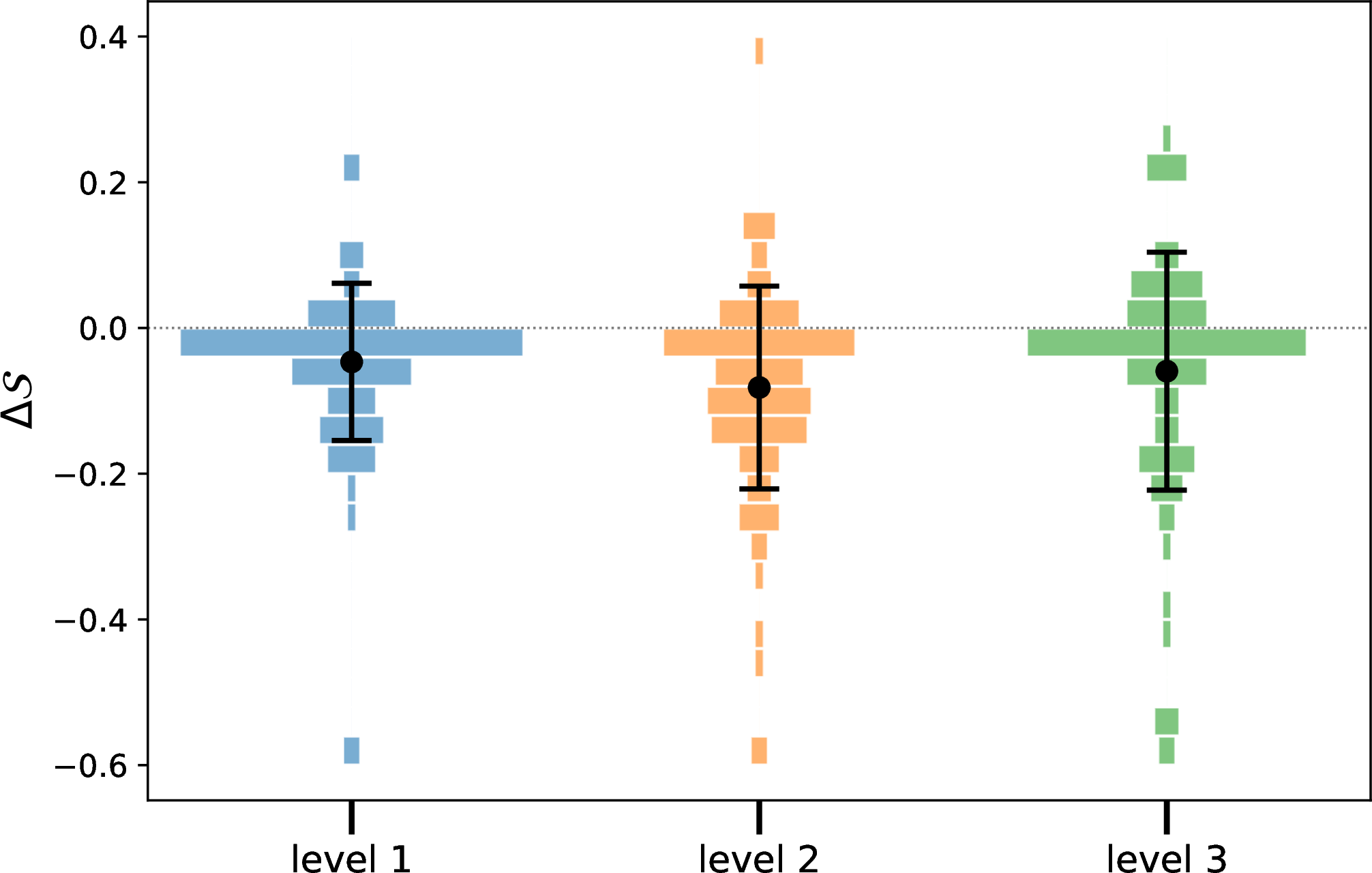
Figure 4 reports the single-step score change \(\Delta\mathcal{S}\) for \(100\) recorded parent–child transitions from round 1 at each prompt assigned mutation level. The distributions are centered close to zero but have slightly negative means for all three levels. This is expected in an exploratory mutation process, where most edits do not immediately improve the decoded fitness, while the positive side of the distribution contains score-improving children that can be retained and propagated by selection. In contrast to Level 1, Level 2 and Level 3 modify higher-level structural choices. These moves are higher-risk, as they require more extensive consistency repairs and can more easily decrease the score in a single step. At the same time, they substantially enlarge the accessible search space and create opportunities to discover better codes that would be inaccessible to purely local mutations.
S4. Quality-Diversity Archive and Parent Selection↩︎
| Seed | Base group | \(A\)-shape / \(B\)-shape | Column factor \(f\) | Note |
|---|---|---|---|---|
| 1 | dihedral \(D_m\) | \(3\times4\) / \(3\times4\) | 25 | |
| 2 | cyclic \(\mathbb{Z}_t\) | \(3\times4\) / \(3\times4\) | 25 | |
| 3 | cyclic \(\mathbb{Z}_t\) | \(2\times4\) / \(2\times4\) | 20 | |
| 4 | dicyclic \(\mathrm{Dic}_m\) | \(3\times4\) / \(3\times4\) | 25 | |
| 5 | dicyclic \(\mathrm{Dic}_m\) | \(3\times4\) / \(3\times4\) | 25 | polynomial entries |
| 6 | dihedral \(D_m\) | \(2\times3\) / \(2\times3\) | 13 | |
| 7 | dicyclic \(\mathrm{Dic}_m\) | \(3\times4\) / \(2\times4\) | 22 | |
| 8 | dihedral \(D_m\) | \(3\times4\) / \(2\times4\) | 22 | |
| 9 | \(\mathbb{Z}_3\times\mathbb{Z}_t\) | \(4\times5\) / \(2\times3\) | 23 | |
| 10 | \(\mathbb{Z}_3\times\mathbb{Z}_t\) | \(3\times4\) / \(3\times4\) | 25 | polynomial entries |
| 11 | \(\mathbb{Z}_3\times\mathbb{Z}_t\) | \(3\times4\) / \(3\times4\) | 25 |
The evolutionary database combines a MAP-Elites quality-diversity archive with an island population model. The two components have different roles. MAP-Elites determines which evaluated programs are retained, while the island model controls how parents are sampled for mutation and helps preserve multiple semi-isolated lineages. Our implementation builds on the OpenEvolve framework [53].
0.0.0.6 Initial seeds.
The archive is initialized with \(11\) scalable lifted-product families spanning four base group families including dihedral \(D_m\), cyclic \(\mathbb{Z}_t\), dicyclic \(\mathrm{Dic}_m\), and \(\mathbb{Z}_3\times\mathbb{Z}_t\) (listed in Table 2). In addition to varying the base group, we adopt protograph shapes of different sizes to further increase the diversity of the seed set. Beyond these scalable families, we also seed a bivariate-bicycle code (\(\mathbb{Z}_{12}\times\mathbb{Z}_{24}\), \(n=576\)) and an A2\(\times\)4/B2\(\times\)4 dicyclic lifted-product seed (\(n=560\)), both with fixed block length below the scoring window (\(n_{\text{min}}=600\)). These seeds score \(0\) and enter the run only as diversity templates.
0.0.0.7 MAP-Elites grid.
Each evaluated program is placed in a MAP-Elites cell according to three descriptor components: its decoder success probability, encoding rate \(k/n\), and inherited seed-lineage label. These descriptor components are discretized into bins, so each program maps to a single cell of a MAP-Elites grid. Each island maintains its own grid. An occupied cell stores only the highest fitness score program whose descriptor falls in that cell. A newly evaluated program replaces the incumbent only if its combined score \(\mathcal{S}\) is higher. The grid thus indexes, for each occupied niche, the best program found there and records which behavioral regions, decoding success, rate, and inherited seed-lineage label the search has covered so far.
0.0.0.8 Island model and migration.
The population is divided into \(N_{\mathrm{isl}}\) islands. At the start of each round, every seed program is placed in its own island, so that one island holds one initial seed and \(N_{\mathrm{isl}}\) equals the number of seeds. Migration is triggered when the island generation counter has advanced by \(20\) since the previous migration event. From each island the top fraction \(\mu=0.05\) by fitness score is copied to its two ring-adjacent neighbors (islands \(i\!\pm\!1 \bmod N_{\mathrm{isl}}\)). To avoid duplication a program migrates at most once. Migration lets strong candidates diffuse across islands while preserving inter-island diversity between migration events.
0.0.0.9 Parent and reference program selection
The database keeps a single global elite archive holding the \(20\) highest scoring programs across all islands. At each step one island is scheduled, and a parent program is sampled following a three-way mixture. (1) Exploitation (\(50\%\)): Parent A is drawn from the global elite archive: candidates are first restricted to the archived programs that originate from the scheduled island, and only if that island contributes none of the \(20\) archive members does the sampler use the full archive, i.e.elites from other islands. Archive candidates are selected by a softmax over fitness, \(w_i \propto \exp\!\left[\frac{\mathcal{S}_i-\max_j \mathcal{S}_j}{T}\right]\), where \(\mathcal{S}_i\) is the fitness score and \(T\) is the softmax temperature. The temperature is annealed geometrically over the run, from \(T_0=1.0\) to \(T_1=0.1\), and \(T(t) = (0.1)^{\,t/T_{\max}}\), where \(t\) is the current iteration and \(T_{\max}=1000\) the total number of iterations. (2) Exploration (\(35\%\)): Parent A is sampled uniformly from the positive-score programs in the scheduled island’s population, falling back to all valid programs in that island if none is positive. (3) Exploitation inside island (\(15\%\)): Parent A is sampled from the scheduled island’s population with linear fitness score weights \(w_i=\max(\mathcal{S}_i,0.001)\). After each mutation, the generated child is inserted into the scheduled island.
At each iteration a small set of reference programs is drawn from the parent’s island to serve as structural context: the top \(3\) positive-score programs in that island, plus one additional program drawn uniformly at random from the same island.
S5. Novelty check↩︎
To prevent the archive from filling with structurally similar codes, we attach to each candidate a lightweight fingerprint of its Tanner graphs. This fingerprint follows the spirit of Weisfeiler–Lehman graph-kernel methods [62], [63]. For new candidates, we compare this fingerprint with those of archived candidates and multiply its fitness score by a novelty penalty factor. For each valid candidate, we sample \(128\) variable nodes, with a fixed seed per block length, so that all codes of the same \(n\) are probed at identical node position. Starting from each sampled variable node, we run a breadth-first search to radius \(3\) in both the \(H_X\) and \(H_Z\) Tanner graphs. At each radius \(r=1,2,3\), we summarize the layer by three key quantities. Local degree: the number of reached nodes of each degree; growth profile: the number of newly reached nodes at each radius \(r\); revisits: number of edges that fold back onto already visited nodes. Each such layer summary is treated as a discrete feature, and we count its occurrences over all sampled roots. After normalization, this gives two feature distributions, \(\phi_X\) and \(\phi_Z\), one for each Tanner graph of \(H_X\) and \(H_Z\).
A new candidate is compared only with archived candidates of the same block length \(n\). For two candidates \(C\) and \(C'\), we define their structural distance as the averaged \(\ell_1\) distance between the two Tanner-graph fingerprints, \[\epsilon(C,C') = \tfrac{1}{2}\,\lVert \phi_X(C)-\phi_X(C')\rVert_1 + \tfrac{1}{2}\,\lVert \phi_Z(C)-\phi_Z(C')\rVert_1 .\] Let \(\epsilon\) denote the distance from the new candidate to its nearest archived neighbour. We then multiply its score by \[\gamma(\epsilon)=1-e^{-\epsilon/\tau}, \qquad \tau=0.01 .\] Thus, candidates whose local Tanner-graph statistics nearly match an existing archive entry are strongly suppressed, whereas structurally distinct candidates are essentially unaffected. If the nearest-neighbour distance satisfies \(\epsilon\le 10^{-9}\), we treat the candidate as an exact fingerprint duplicate and reject it by setting \(\gamma=0\).
S6. Finite-Size Scaling of discovered codes↩︎
We also examine how the discovered constructions behave as the block length is varied. We re-evaluate four scalable elite constructions from round 3: two high-scoring dicyclic codes from the \(\mathcal{C}_{\mathrm{score}}\) set, ranked first and second (denote as R3Elite01 and R3Elite02), and two high decoder success rate codes from the \(\mathcal{C}_{p_L}\)
set, also ranked first and second (denote as R3EliteP01 and R3EliteP02). We remark that R3Elite01 and R3Elite02 belong to the dicyclic family \(\mathrm{Dic}_m\) with the
block size \(n=136m\). R3EliteP01 and R3EliteP02 belong to abelian \(\mathbb{Z}_t\!\times\!\mathbb{Z}_2\) with \(n=50t\).
Each construction is instantiated at admissible \(n\), and the code-capacity logical failure rate \(p_L\) is measured with \(10^{6}\) Monte-Carlo shots per point under the BP+OSD decoder (iteration limit \(5000\), OSD-CS order \(4\)). The results are summarized in Fig. 5.
![Figure 5: Block-length dependence of the logical failure rate. (a)–(c) p_L versus n at physical error rates p=0.05,0.06,0.07 for the two dicyclic (\mathrm{Dic}_m, n=136m) and two abelian (\mathbb{Z}_t\!\times\!\mathbb{Z}_2, n=50t) families. 10^{6} shots per point, error bars are 95% Clopper–Pearson confidence intervals [60]. (d) Encoding rate k/n versus n for the same constructions. For the abelian family only the non-cyclic sizes (t even) are shown. The cyclic sizes (t odd, where \mathbb{Z}_t\!\times\!\mathbb{Z}_2\cong\mathbb{Z}_{2t}) collapse to a degenerate small-distance code and are excluded.](/article/2606.24808/diffn_pL_vs_n.png "fig:")
The dependence on block length is not smoothly monotone. Individual sizes can deviate sharply from their neighbors, for example R3Elite02 at \(n=1088\) and \(n=2176\), and a
milder bump near \(n=1904\) shared by both dicyclic codes. They reflect the finite-size sensitivity of the particular combination of group parameter and local group-algebra entries, whose decoded performance can vary
non-monotonically with \(m\). Despite these size-dependent fluctuations, the top-score elite families still show an overall finite-size suppression trend at \(p=0.05\) and \(p=0.06\). Across the accessible range, increasing \(n\) generally lowers the logical failure rate before \(n = 2176\). At \(p=0.07\), the suppression is much weaker: the dicyclic families remain around \(p_L\sim10^{-2}\) and the abelian families around \(p_L\sim10^{-3}\), with little
systematic improvement as \(n\) grows.
On the other hand, R3EliteP01 and R3EliteP02 achieve their best performance near \(n\simeq1500\), the block-length region targeted by the search. Their performance does not continue to improve
when extrapolated to larger \(n\). We note that for \(\mathbb{Z}_t\!\times\!\mathbb{Z}_2\) the group is non-cyclic only when \(t\) is even. At odd \(t\) it satisfies \(\mathbb{Z}_t\!\times\!\mathbb{Z}_2\cong\mathbb{Z}_{2t}\) and degenerates to a cyclic group.
Panel (d) shows that the two families occupy different regions of the rate–decoder performance tradeoff. The dicyclic codes maintain a relatively high encoding rate, \(k/n\approx0.13\), across the scanned range, whereas the abelian codes have a lower rate, \(k/n\approx0.05\). At comparable block lengths, the lower-rate abelian codes achieve smaller logical failure rates, as expected from their larger redundancy.
S7. Protographs of the specific codes mentioned in the main text↩︎
Each LP code is obtained from two protograph matrices \(A\in G^{m_A\times n_A}\) and \(B\in G^{m_B\times n_B}\) over a finite group \(G\). Each entry below is a group element written multiplicatively in the stated generators with \(e\) the identity. Here we present the codes listed in Table 1 and Fig. 3.
R1Elite01(\(G=\mathbb{Z}_3\times\mathbb{Z}_{14}\), abelian, \([[1428,186,\le 18]]\))↩︎
Generators \(x,y\): \(x^{3}=y^{14}=e,\;xy=yx\), \(|G|=42\).
\[A=\begin{pmatrix} x^{2}y^{8} & xy^{10} & x^{2}y^{6} & e & x^{2}y^{10} \\ xy^{4} & x^{2}y^{8} & xy^{7} & x^{2}y^{7} & xy^{9} \\ y^{13} & x^{2}y^{4} & xy^{13} & y^{4} & y^{5} \end{pmatrix},\qquad B=\begin{pmatrix} y^{10} & y^{6} & x & y^{5} & x^{2}y^{6} \\ y^{6} & xy & y^{9} & y^{5} & xy^{12} \\ y^{3} & y^{3} & y & x^{2}y^{2} & y^{7} \end{pmatrix}.\]
R1Elite02(\(G=\mathbb{Z}_2\times\mathbb{Z}_2\times \mathbb{Z}_{11}\), abelian, \([[1496,198,\le 16]]\))↩︎
Generators \(a,b,c\): \(a^{2}=b^{2}=c^{11}=e\), \(|G|=44\).
\[A=\begin{pmatrix} c^{5} & ac^{7} & c^{2} & c^{6} & abc^{2} \\ abc^{2} & bc^{3} & bc^{4} & bc^{10} & ac^{6} \\ c & ac^{10} & c^{3} & bc & c^{9} \end{pmatrix},\qquad B=\begin{pmatrix} abc^{4} & abc^{3} & e & b & b \\ ac^{3} & abc^{2} & bc^{8} & abc^{4} & c^{7} \\ bc^{4} & ac & ac^{2} & ac^{7} & bc^{5} \end{pmatrix}.\]
R2Elite01(\(G=\mathrm{Dic}_{11}\), non-abelian, \([[1496,194,\le 20]]\))↩︎
Generators \(r,s\): \(r^{22}=e,\;s^{2}=r^{11},\;srs^{-1}=r^{-1}\), \(|G|=44\).
\[A=\begin{pmatrix} r^{8} & r & r^{15} \\ r^{7}s & r^{2} & r^{18}s \\ r^{4} & r & e \\ r^{3}s & r^{3} & r^{2}s \\ r & r^{3} & r^{5} \end{pmatrix},\qquad B=\begin{pmatrix} r^{11} & s & r^{9} \\ r^{12} & e & r^{11} \\ r^{10} & r^{3}s & r^{16} \\ r^{10} & r^{3} & r^{18} \\ r^{9} & r^{6}s & rs \end{pmatrix}.\]
R2Elite02(\(G=\mathrm{D}_{22}\), non-abelian, \([[1496,198,\le 16]]\))↩︎
Generators \(r,s\): \(r^{22}=e,\;s^{2}=e,\;srs^{-1}=r^{-1}\), \(|G|=44\).
\[A=\begin{pmatrix} r^{12} & r^{3}s & r^{17} \\ r^{8} & s & r^{15} \\ r^{4}s & r^{20}s & r^{13}s \\ e & r^{17}s & r^{11} \\ r^{19} & r^{14} & r^{9} \end{pmatrix},\qquad B=\begin{pmatrix} r^{21} & r & r^{10} \\ r^{12} & e & r^{3} \\ r^{3} & r^{14} & r^{3} \\ rs & r^{6}s & r^{19} \\ r^{14} & r^{5} & r^{11} \end{pmatrix}.\]
R3Elite01(\(G=\mathrm{Dic}_{11}\), non-abelian, \([[1496,192,\le 16]]\))↩︎
Generators \(r,s\): \(r^{22}=e,\;s^{2}=r^{11},\;srs^{-1}=r^{-1}\), \(|G|=44\).
\[A=\begin{pmatrix} r^{14}s & rs & r^{10}s & r^{19} & r^{6} \\ r^{5}s & r^{21}s & r^{15} & r^{9} & r^{3}s \\ r^{18}s & r^{19} & r^{20}s & r^{21}s & e \end{pmatrix},\qquad B=\begin{pmatrix} r^{19}s & r^{18}s & r^{9} & r^{19} & r^{8}s \\ r^{2}s & r^{21} & r^{3}s & r^{11} & rs \\ r^{12}s & r^{17} & r^{18} & r^{15}s & r^{12}s \end{pmatrix}.\]
R3Elite02(\(G=\mathrm{Dic}_{11}\), non-abelian, \([[1496,198,\le 14]]\))↩︎
Generators \(r,s\): \(r^{22}=e,\;s^{2}=r^{11},\;srs^{-1}=r^{-1}\), \(|G|=44\).
\[A=\begin{pmatrix} r^{16} & r^{17}s & r^{18} & s & r^{2} \\ r^{17}s & rs & r^{2}s & r^{4}s & r^{6}s \\ r^{18} & r^{2}s & r^{5} & r^{8}s & r^{11} \end{pmatrix},\qquad B=\begin{pmatrix} r^{15} & r^{9}s & r & r^{10}s & r^{3} \\ r^{11} & r^{5} & r^{15} & r^{9} & r^{3} \\ r^{7} & r^{2}s & r^{13} & r^{8}s & r^{3} \end{pmatrix}.\]
R3EliteP01(\(G=\mathbb{Z}_{30}\times\mathbb{Z}_2\), abelian, \([[1500,81,\le 18]]\))↩︎
Generators \(x,y\): \(x^{30}=y^{2}=e,\;xy=yx\), \(|G|=60\).
\[A=\begin{pmatrix} x^{22} & x^{17} & x^{19} & x^{21} \\ x^{23}y & x^{11}y & x^{22}y & x^{10}y \\ x & x^{28} & x^{2} & x^{29} \end{pmatrix},\qquad B=\begin{pmatrix} x^{28}y & x^{11}y & x^{7}y & x^{17}y \\ x^{26} & x^{18}y & x^{29} & x^{21}y \\ x^{5}y & x^{28}y & x^{21}y & x^{25}y \end{pmatrix}.\]
R3EliteP02(\(G=\mathbb{Z}_{30}\times\mathbb{Z}_2\), abelian, \([[1500,76,\le 20]]\))↩︎
Generators \(x,y\): \(x^{30}=y^{2}=e,\;xy=yx\), \(|G|=60\).
\[A=\begin{pmatrix} x^{6}y & x^{6} & x^{6}y & x^{6} \\ e & x & x^{2} & x^{26} \\ x^{24}y & x^{26} & x^{21}y & x^{23} \end{pmatrix},\qquad B=\begin{pmatrix} x^{29}y & x^{13} & x^{8}y & x^{3} \\ x^{10} & x^{6} & x^{2} & x^{28} \\ x^{2}y & x^{29} & x^{26}y & x^{12} \end{pmatrix}.\]
Here we list the full protograph matrices of the codes used to illustrate the three mutation levels in Fig. 2 (a). These codes follow the naming convention DemoL\(\ell\)Parent / DemoL\(\ell\)Child, where \(\ell\in\{1,2,3\}\) labels the mutation level of the corresponding
parent-to-child step, and Parent (Child) denotes the protograph matrices \(A,B\) of the code before (after) the mutation is applied.
DemoL1Parent(\(G=\mathrm{Dic}_{15}\), non-abelian, \([[1500,74]]\))↩︎
Generators \(r,s\): \(r^{30}=e,\;s^{2}=r^{15},\;srs^{-1}=r^{-1}\), \(|G|=60\).
\[A=\begin{pmatrix} r^{10}s & r^{24} & r^{2}s & r^{13}s \\ r^{18} & r^{4}s & r^{18}s & r^{26} \\ r^{28} & r^{13}s & r^{28}s & r^{10}s \end{pmatrix},\qquad B=\begin{pmatrix} r^{4}s & r^{14}s & r^{27} & r^{4}s \\ r^{11} & r^{19} & r^{3}s & r^{15}s \\ r^{12} & r^{27}s & r^{9} & r^{22}s \end{pmatrix}.\]
DemoL1Child(\(G=\mathrm{Dic}_{15}\), non-abelian, \([[1500,79]]\))↩︎
Generators \(r,s\): \(r^{30}=e,\;s^{2}=r^{15},\;srs^{-1}=r^{-1}\), \(|G|=60\).
\[A=\begin{pmatrix} r^{13}s & r^{21}s & s & r^{8}s \\ r^{18} & r^{27} & r^{7} & r^{16} \\ r^{22}s & r^{4}s & r^{14}s & r^{24}s \end{pmatrix},\qquad B=\begin{pmatrix} r^{4} & r^{17}s & e & r^{12}s \\ r^{9}s & r^{24} & r^{7} & r^{21} \\ r^{16} & s & r^{15} & s \end{pmatrix}.\]
DemoL2Parent(\(G=\mathrm{Dic}_{15}\), non-abelian, \([[1500,81]]\))↩︎
Generators \(r,s\): \(r^{30}=e,\;s^{2}=r^{15},\;srs^{-1}=r^{-1}\), \(|G|=60\).
\[A=\begin{pmatrix} r^{29}s & e & r^{6}s & r^{12} \\ r^{28} & r^{6}s & r^{13} & r^{29}s \\ r^{10}s & r^{12} & r^{20}s & r^{28}s \end{pmatrix},\qquad B=\begin{pmatrix} r^{28}s & r^{2}s & r^{7}s & r^{12}s \\ rs & r^{7} & r^{13}s & r^{19} \\ r^{5}s & r^{12}s & r^{19}s & r^{26}s \end{pmatrix}.\]
DemoL2Child(\(G=\mathrm{Dic}_{11}\), non-abelian, \([[1496,198]]\))↩︎
Generators \(r,s\): \(r^{22}=e,\;s^{2}=r^{11},\;srs^{-1}=r^{-1}\), \(|G|=44\).
\[A=\begin{pmatrix} r^{7} & r & r^{15} \\ r^{6}s & r^{2} & r^{18}s \\ r^{5} & r^{2} & e \\ r^{3}s & r^{3} & r^{2}s \\ r^{2} & r^{3} & r^{5} \end{pmatrix},\qquad B=\begin{pmatrix} r^{11} & s & r^{9} \\ r^{11} & e & r^{11} \\ r^{10} & r^{3}s & r^{16} \\ r^{11} & r^{3} & r^{18} \\ r^{9} & r^{6}s & e \end{pmatrix}.\]
DemoL3Parent(\(G=\mathbb{Z}_{2}\times \mathbb{Z}_{2}\times\mathbb{Z}_{11}\), abelian, \([[1496,176]]\))↩︎
Generators \(a,b,c\): \(a^{2}=b^{2}=e,\;c^{11}=e,\;ab=ba,\;ac=ca,\;bc=cb\), \(|G|=44\).
\[A=\begin{pmatrix} e & a + c & b & ab & ac + ab \\ bc & e & ab + a + bc & c & a \\ b + ab & ac & e & bc + c & ab \end{pmatrix},\qquad B=\begin{pmatrix} e & c & b & ac & ab + a \\ a + b & e & c & abc & b \\ bc & e + ab & a & b & abc + c \end{pmatrix}.\]
DemoL3Child(\(G=(\mathbb{Z}_{2}\times \mathbb{Z}_{2})\rtimes\mathbb{Z}_{10}\), non-abelian, \([[1360,160]]\))↩︎
Generators \(a,b,c\): \(a^{2}=b^{2}=e,\;ab=ba,\;c^{10}=e,\;cac^{-1}=b,\;cbc^{-1}=a\), \(|G|=40\). (symbolic entries remain the same.)
\[A=\begin{pmatrix} e & a + c & b & ab & ac + ab \\ bc & e & ab + a + bc & c & a \\ b + ab & ac & e & bc + c & ab \end{pmatrix},\qquad B=\begin{pmatrix} e & c & b & ac & ab + a \\ a + b & e & c & abc & b \\ bc & e + ab & a & b & abc + c \end{pmatrix}.\]