Reweighting Underlying Event and Colour Reconnection parameter variations in S
June 23, 2026
1 Introduction↩︎
Detailed particle-level simulations that encapsulate theoretical expectations are a central ingredient to the analysis and interpretation of data at high-energy collider experiments. The widely used general-purpose Monte Carlo event generators (MCEGs) H [1], [2], P [3]–[5], and S [6]–[8] provide detailed and complete particle-level predictions, accounting for the complex evolution from partonic hard scatterings to hadronic final states by combining first-principles perturbative QCD calculations with phenomenological models for non-perturbative (NP) effects [9], [10].
The robust quantification of inherent theoretical uncertainties in the underlying physics models is crucial for precision phenomenology and the correct interpretation of data, including, for example, evidence for new phenomena or constraints on them. In the perturbative regime, on-the-fly event reweighting techniques facilitate the efficient evaluation of uncertainties in both the hard scattering matrix elements and the subsequent parton shower, as they arise from variations in the strong coupling, scale choices, and parton-density functions (PDFs) [11]–[13]. These techniques have become indispensable for the estimation of perturbative uncertainties and have eliminated the computationally costly need to regenerate events with varying settings.
However, many phenomenologically important uncertainties originate from the NP modelling of the underlying event, hadronisation, and (soft) colour reconnections. These models depend on empirical parameters that must be calibrated, “tuned”, to existing collider data. This is typically achieved through global fits using tools such as Professor [14] and Apprentice [15] or, more recently, the technique of History Matching (HM) using Bayes Linear Emulators [16]1. Variations within the best-fit regions of the model-parameter space resulting from the tuning can be used to estimate model-inherent uncertainties or to study the sensitivity of physical observables on the parameters. In practice, however, producing dedicated simulation runs for large multi-dimensional parameter-space samples is computationally prohibitive; this frequently results in a rather superficial assessment of such parametric uncertainties obtained, e.g., from direct comparison of two MCEGs or of different tunes of the same MCEG.
This paper aims to address this problem. In particular, we introduce and validate a method that offers a promising route to accelerated non-perturbative model explorations, parameter-sensitivity studies and uncertainty estimation. It allows the propagation of parameter-uncertainty variations, e.g.from a wave of HM, without the need for multiple event-simulation runs. While initial steps towards reweighting techniques for hadronisation models have recently been reported by the MLHad collaboration [19]–[21] for the Lund-string fragmentation in P, such implementations do not yet exist for Multiple Parton Interactions (MPI) and Colour Reconnection (CR) models. In this work, we present the first implementation of on-the-fly reweighting for MPI and CR parameters within S, extending the scope of existing perturbative reweighting frameworks to all key non-perturbative components of event generation. The resulting approach provides in-situ derived alternative event weights corresponding to specified variations of model parameters. This enables the efficient and robust exploration of the parameter space. Our new method significantly accelerates the generation of alternative generator predictions, reduces the storage requirements for the samples, and alleviates post-processing efforts, for example event analyses or detector simulations, because, effectively, only one event sample is generated, where vectors of relative event-by-event weights capture the effect of the parameter variations.
Our paper is structured as follows: In Section 2 we review the S MPI and CR models and outline the reweighting approach. In Section 3 we demonstrate the capabilities of this new functionality by performing a tuning of the S MPI and CR models to LHC data at \(\sqrt{s}=7\,\text{TeV}\) using Apprentice in conjunction with the reweighting framework, covering a broad parameter space with a single dedicated run. We furthermore illustrate the application of the reweighting approach to assess the energy extrapolation of dimensionful model parameters. We conclude in Section 4 with a summary and an outlook.
2 Setting the scene↩︎
Following the standard collinear-factorisation approach for modelling hadron–hadron collisions, single \(2\to n\) partonic-scattering processes are considered, with one initial-state parton extracted from each of the incident hadrons. In MCEGs this primary or hard-process configuration is then subjected to parton-shower evolution and hadronisation. At low scales of a few \(\Lambda_{\rm QCD}\), the partons emerging from the shower will fragment into primary hadrons, some of which will decay further. This process has been studied at exquisite accuracy at L, mainly at the \(Z\)-pole, and, as a consequence, the non-perturbative parameters describing hadronisation are usually calibrated to these data, cf.for example [16], [17], [22]–[24]. However, more recently, data from HERA, flavour factories, and the LHC have also been included in fragmentation-model tuning [25], [26].
When attempting to use this to describe final-state observables at hadron colliders, there is striking evidence for additional effects. There are certainly two contributions that can be distinguished. Firstly, the incident partons can carry a small but non-vanishing transverse momentum relative to the beam axis, often called intrinsic-\(k_T\). Secondly, the remnants of the incident hadrons can interact, resulting in additional final-state hadronic activity, originally referred to as jet-pedestal effect [27], nowadays known as the Underlying Event (UE) [28]–[33]. We here focus explicitly on the second component. The modelling of the UE is treated differently in MCEGs [9], [10]. To describe the UE, Multiple Parton Interactions (MPIs), i.e.secondary \(2\to 2\) QCD scatters, are introduced, that also undergo parton-shower evolution and hadronisation. In Section 2.1 we will give a brief review of the model and illustrate how its inherent parameters can be reweighted on-the-fly.
The parton-shower evolution of the primary and secondary scatterings is accomplished in the large-\(N_c\) approximation2. This results in planar colour flows only, where each quark and gluon has well defined colour partner(s), facilitating the transition from partons to colour-neutral hadronic states (i.e., the clusters in Ahadic) at lower scales [36]. While, typically, the hard process is evaluated using \(N_c=3\), the above treatment requires the (probabilistic) assignment of a planar colour flow that seeds the subsequent shower evolution, in which subleading colour configurations in the splitting processes are neglected.
In the presence of secondary scatterings, neither the colour structure of the beam remnants nor the colour correlations between the MPI scatters and the hard process are uniquely defined. To at least approximately include subleading perturbative configurations, to effectively model the exchange of non-perturbative emissions, and to account for alternative beam-remnant colour assignments, MCEGs include the option of Colour Reconnections (CRs), i.e.the probabilistic rearrangement of colour–anti-colour partners. In Section 2.2 we detail the model used in S and how its parameters can be reweighted on-the-fly.
The subtle interplay of the models for MPIs and CRs in affecting the final-state hadronic activity implies that they cannot be calibrated with experimental data in isolation. Accordingly, in Section 3 we will consider two scenarios for the tuning, one with MPI only and one with both MPI and CR enabled.
2.1 Reweighting the Underlying Event in S↩︎
A comprehensive understanding of the model’s parameter dependences is essential to achieve the correct reweighting of the MPI model across a varied parameter space. The following is a brief review of the MPI model in S, which essentially re-implements the Sjöstrand–van-Zijl (SZ) model [37].
We begin by specifying the geometrical configuration for the incident beam particles participating in the MPIs in S. The hadronic matter distribution of each incident hadron, parametrised by form factors \(\rho(r)\), is assumed to be spherically symmetric and independent of parton flavour or longitudinal momentum fraction 3. In parallel to the SZ model, S models this as a superposition of two Gaussian distributions, \[\rho(r) = \sum_{i=1}^{2} \frac{\alpha_i}{(\sqrt{\pi} R_i)^3} \exp\left(-\frac{r^2}{R_i^2}\right)\,,\] where \(R_i/\sqrt{2}\) denote the Gaussian widths (w.l.o.g.we assume \(R_1 \leq R_2\)) and \(\alpha_i\) are the fractional weights satisfying \(\alpha_1 + \alpha_2 = 1\). The normalisation is chosen such that \(\int {\rm d}^3x\, \rho(r) = 1\).
Given these single-hadron matter profiles, the geometry of a hadron–hadron collision is encoded in the time-integrated spatial overlap of the two distributions. For two hadrons with density profiles \(\rho_1(r)\) and \(\rho_2(r)\) moving along the \(\pm z\)-direction separated by the transverse impact parameter \(b\), the overlap function reads \[\begin{align} O(b) \;=\; \int {\rm d}t \int {\rm d}^3x \rho_1(x, y, z) \rho_2(x, y, z - \sqrt{b^2 + t^2}) \;=\; \frac{1}{\pi} \sum_{i,j=1}^{2} \frac{\alpha_i \alpha_j}{R_i^2 + R_j^2} \exp\left(-\frac{b^2}{R_i^2 + R_j^2}\right)\,. \label{eq:overlap} \end{align}\tag{1}\] The overlap function is normalised to \(\int {\rm d}^2b\, O(b) = 1\) and thus quantifies the probability density for parton encounters at a given impact parameter \(b\). It enters the calculation of the perturbative QCD cross section for parton–parton interactions, as \[\sigma_{ij \to kl} = \int {\rm d}p_\perp^2 \, {\rm d}^2b \, {\rm d}\xi_1 \, {\rm d}\xi_2 \, O(b) \, f_i(\xi_1, \mu_F^2) \, f_j(\xi_2, \mu_F^2) \, \frac{{\rm d}\hat{\sigma}_{ij \to kl}(\mu^2_R)}{{\rm d}p_\perp^2}\,.\] The factorisation and renormalisation scales are set to \(\mu_{F,R}^2 = c_{F,R}^2\, p_\perp^2\), with prefactors \(c_{F,R}\) and \(p_\perp\) denoting the transverse momentum of the partonic scattering. To avoid the divergence at \(p_\perp \to 0\), a minimum transverse momentum cutoff \(p_{\perp,\min}\) is introduced, below which no perturbative scatterings are considered. Therefore, the total hard scattering cross section is given as a sum over all contributing partonic channels \[\sigma_{\rm hard}(p_{\perp,\min}) = \sum_{ijkl} \int_{p_{\perp,\min}^2}^{\infty} {\rm d}p_\perp^2 \int {\rm d}^2b \, {\rm d}\xi_1 \, {\rm d}\xi_2 \, O(b) \, f_i(\xi_1, \mu_F^2) \, f_j(\xi_2, \mu_F^2) \, \frac{{\rm d}\hat{\sigma}_{ij \to kl}(\mu^2_R)}{{\rm d}p_\perp^2}\,. \label{eq:sigma95hard}\tag{2}\] While the sharp cutoff removes the formal divergence, it enforces an abrupt and somewhat artificial separation between “hard” and “soft” scatterings. To obtain a smoother transition for small transverse momenta, the partonic cross section is further regularised by a damping factor \[\frac{p_\perp^4}{(p_\perp^2 + p_{\perp,0}^2)^2}\,,\] and the strong coupling \(\alpha_s(\mu_R^2)\) is evaluated at an effective scale \(\mu_R^2 = c_R^2(p_\perp^2 + p_{\perp,0}^2)\).
The average number of hard interactions above the transverse-momentum threshold \(p_{\perp,\min}\) is given by the ratio of the perturbative cross section 2 and the non-diffractive hadronic cross section, \[\langle n(p_\perp > p_{\perp,\min}) \rangle = \frac{\sigma_{\rm hard}(p_{\perp,\min}, p_{\perp,0})}{\sigma_{\rm ND}}\,.\] Assuming independent parton–parton scatterings, the number of interactions at a given impact parameter follows a Poisson distribution with mean \(\bar{n}(b, p_{\perp,\min})\). Following this, the probability for two passing hadrons to undergo a collision (i.e., at least one parton–parton interaction above \(p_{\perp,\min}\)) is obtained from Poissonian statistics as \[P_{\rm int}(b, p_{\perp,\min}) = 1 - \exp\bigl(-\bar{n}(b, p_{\perp,\min})\bigr)\,, \label{eq:pint}\tag{3}\] and the average number of interactions at a given \(b\) in a non-diffractive event is therefore \[\langle n(b, p_{\perp,\min}) \rangle = \frac{\bar{n}(b, p_{\perp,\min})}{P_{\rm int}(b, p_{\perp,\min})}\,.\] Integrating over all impact parameters then recovers the overall average number of interactions \[\langle n \rangle = \frac{\int {\rm d}^2b \, \langle n(b, p_{\perp,\min}) \rangle P_{\rm int}(b, p_{\perp,\min})}{\int {\rm d}^2b \, P_{\rm int}(b, p_{\perp,\min})} = \frac{\int {\rm d}^2b \, \bar{n}(b, p_{\perp,\min})}{\int {\rm d}^2b \, P_{\rm int}(b, p_{\perp,\min})} = \frac{\sigma_{\rm hard}}{\sigma_{\rm ND}}\,.\] Comparison with the hard cross section (2 ) suggests that the impact-parameter-dependent MPI rate is given by \[\bar{n}(b, p_{\perp,\min}) = O(b) \,\sum_{ijkl} \int_{p_{\perp,\min}^2}^{\infty} {\rm d}p_\perp^2 \, {\rm d}\xi_1 \, {\rm d}\xi_2 \, f_i(\xi_1, \mu_F^2) \, f_j(\xi_2, \mu_F^2) \, \frac{{\rm d}\hat{\sigma}_{ij \to kl}(\mu^2_R)}{{\rm d}p_\perp^2}\,.\] The integrated interaction probability must therefore equal the non-diffractive cross section \[\int {\rm d}^2b \, P_{\rm int}(b) = \int {\rm d}b\, 2\pi b \left[1 - \exp\bigl(-\bar{n}(b, p_{\perp,\min})\bigr)\right] = \sigma_{\rm ND}\,. \label{eq:sigma95nd}\tag{4}\] This expression establishes the connection between the matter-distribution parameters and the observable MPI rates. In order to satisfy this relation, the matter-distribution widths are tuned via a scaling factor \(R^{\rm eff}_i = k \cdot R_i\) 4.
For the actual event simulation, multiple parton scatters are generated in an ordered sequence of decreasing \(p_\perp\). Similar to the treatment of multiple emissions in parton showers, a Sudakov-like form factor encodes the suppression of additional interactions. The exponential probability for no scattering between two successive transverse-momentum scales is thus given by \[\Delta(b) = \exp\left(-\int_{p_{\perp,\text{next}}^2}^{p_{\perp,\text{prev}}^2} \mathrm{d}p_\perp^2 \int \mathrm{d}\xi_1 \,\mathrm{d}\xi_2 \, O(b) \sum_{ijkl} f_i(\xi_1, \mu_F^2)\, f_j(\xi_2, \mu_F^2)\, \frac{\mathrm{d}\hat{\sigma}_{ij\to kl}(\mu_R^2)}{\mathrm{d}p_\perp^2}\right)\,.\] The generation of MPIs proceeds via a downward evolution in \(p_\perp\), starting from a maximum scale set by the hard process, by solving the Sudakov form factor equation for the next lower \(p_\perp\) scale. In practice, an integrable overestimator is used to propose a new trial \(p_\perp\), which is then accepted or rejected based on the true integrand, called the Sudakov Veto Algorithm (SVA) [39]. This procedure is iterated until the transverse momentum falls below the minimum cutoff \(p_{\perp,\min}\), at which point no further hard interactions are generated 5.
This implementation suggests to split the reweighting factor for MPI model-parameter variations into two components: the first factor \(w_b\) accounts for a modified impact-parameter sampling and the second factor \(w_{\rm Sudakov}\) captures the variations of the Sudakov factors at a given impact parameter (and thus a varied MPI multiplicity). Following this, each event will receive a total weight of \[w_i = (w_b)_i \cdot (w_{\rm Sudakov})_i\] for the parameter variation \(i\). The computation of the impact-parameter reweighting factor \(w_b\) is straightforward. Given an original impact parameter \(b\) sampled from the overlap function \(O(b; \vec{p}_0)\) with parameter set \(\vec{p}_0\), the modified weight for a new parameter set \(\vec{p}_i\) is given by the ratio of the overlap functions evaluated at the same impact parameter \[(w_b)_i = \frac{O(b; \vec{p}_i)}{O(b; \vec{p}_0)}\,. \label{eq:wb}\tag{5}\]
For the Sudakov reweighting factor \(w_{\rm Sudakov}\), the procedure is more involved. As the overestimator used in the SVA depends on the MPI parameters, using the maximum overestimator across all variations is necessary to ensure the validity of the SVA for all parameter sets. With this rescaling, the reweighting factor can be constructed from each accepted and rejected secondary scattering in the event-generation sequence. For each proposed trial \(p_\perp\), the acceptance probability \(\mathcal{P}^{\rm acc}\) of a parameter variation is given by the ratio of the true integrand for the varied and original parameter sets multiplied by the acceptance probability of the original parameter set \[\begin{align} \mathcal{P}^{\rm acc}_i(p_\perp) =&\: \frac{O(b; \vec{p}_i) \sum_{ijkl} f_i(\xi_1, \mu_F^2) \, f_j(\xi_2, \mu_F^2) \, \frac{{\rm d}\hat{\sigma}_{ij \to kl}}{{\rm d}p_\perp^2}(\mu^2_R; \vec{p}_i)}{{\rm overestimator}(p_\perp)} \nonumber\\ =&\: \mathcal{P}^{\rm acc}_0(p_\perp) \cdot \frac{O(b; \vec{p}_i) \sum_{ijkl} f_i(\xi_1, \mu_F^2) \, f_j(\xi_2, \mu_F^2) \, \frac{{\rm d}\hat{\sigma}_{ij \to kl}}{{\rm d}p_\perp^2}(\mu^2_R; \vec{p}_i)}{O(b; \vec{p}_0) \sum_{ijkl} f_i(\xi_1, \mu_F^2) \, f_j(\xi_2, \mu_F^2) \, \frac{{\rm d}\hat{\sigma}_{ij \to kl}}{{\rm d}p_\perp^2}(\mu^2_R; \vec{p}_0)}\,. \end{align}\] Consequently, for an accepted partonic scatter at scale \(p_\perp\) the Sudakov reweighting factor receives a contribution of \[q_i^{\rm acc}(p_\perp) = \frac{\mathcal{P}^{\rm acc}_i(p_\perp)}{\mathcal{P}^{\rm acc}_0(p_\perp)}\,,\] and for each rejected interaction the contribution is given by \[q_i^{\rm rej}(p_\perp) = \frac{1 - \mathcal{P}^{\rm acc}_i(p_\perp)}{1 - \mathcal{P}^{\rm acc}_0(p_\perp)}\,.\] For an event with several accepted and rejected secondary scatterings, the total Sudakov reweighting factor is given by the product of all contributions.
Reweighting is supported for all key parameters of the MPI model introduced above. Specifically, these include the hadronic-matter distribution parameters \(R_1\), \(R_2\), and \(\alpha_1\) that directly influence the overlap function \(O(b)\). The non-diffractive cross section can be rescaled by a normalisation factor \(\sigma_{\rm ND}^{\rm norm}\) to increase or decrease the MPI rate, which through the constraint (4 ) induces a corresponding rescaling \(k\) of the effective Gaussian widths and thereby modifies the overlap.
Variations in these four parameters consequently affect both the impact-parameter distribution and the Sudakov factors through variations of \(O(b)\). Additionally, the model supports variations of the transverse-momentum scales \(p_{\perp,0}\) (controlling the low-\(p_\perp\) spectrum shape) and \(p_{\perp,\min}\) (setting the phase-space boundary of \(\sigma_{\rm hard}\)), with variations in either of these two parameters affecting \(O(b)\) through a change in the \(k\) factor, and directly modifying the Sudakov suppression factors through the so altered MPI acceptance probabilities.
A technical caveat applies to \(p_{\perp,\min}\). For this parameter only upward variations (i.e., increasing the \(p_\perp\) threshold to exclude softer MPIs) are possible, since events generated with an original higher cutoff simply do not fill the phase space and hence cannot be reweighted. However, for a trial \(p_\perp\) below the varied cutoff, the acceptance probability is 0, i.e. \[\mathcal{P}^{\rm acc}_i(p_\perp < (p_{\perp,\min})_i) = 0\,, \label{eq:ptmin95acc}\tag{6}\] ensuring that events with an accepted MPI below the varied cutoff receive a total weight of 0.
Inspired by the Donnachie–Landshoff model for the scaling of the total hadronic cross sections [40], the energy dependence of \(p_{\perp,0}\) and \(p_{\perp,\min}\) is parametrised as \[\label{eq:pts} p_{\perp,0}(s) = p_{\perp,0}^{\rm ref} \left(\frac{s}{s_{\rm ref}}\right)^{\eta}\,, \quad p_{\perp,\min}(s) = p_{\perp,\min}^{\rm ref} \left(\frac{s}{s_{\rm ref}}\right)^{\eta}\,,\tag{7}\] where \(s_{\rm ref}\) is a reference collision-energy scale, and \(\eta\) controls the energy scaling. Variations in \(\eta\) are also supported by the reweighting procedure, as this simply amounts to variations in \(p_{\perp,0}\) and \(p_{\perp,\min}\).
Once the generation of MPIs and subsequent showers have terminated for a single event, the resulting parton configuration must be hadronised, introducing an observable dependence on how colour quantum numbers (in the \(N_c\to\infty\) limit) are distributed over the partons. Realising that for each scatter such colour assignments are more or less straightforward, the relevant question therefore concerns the distribution of colours between the individual parton scatters and, ultimately, with the spectator partons inside the beam remnants.
In S, this problem is solved by assigning colours iteratively. Initially, each individual scattering event undergoes parton showering with the corresponding colour assignments. Once the shower terminates the colours of the two resulting initial-state partons will be redefined such that they are colour-connected to the two initial-state partons of the previous scatter in each hadron. As a consequence this leads to colour-connections between the final-state partons of subsequent MPIs. As a final step, S assigns spectator partons – and, in particular, diquarks in the case of incident baryons – in each of the beam remnants to ensure their correct flavour quantum numbers. These spectator partons will also carry the “trailing” disconnected colours.
| Parameter | Description | Name (in run card) |
|---|---|---|
| \(R_1\) | Gaussian width of core matter distribution | MATTER_RADIUS_1 |
| \(R_2\) | Gaussian width of halo matter distribution | MATTER_RADIUS_2 |
| \(\alpha_1\) | Fractional weight of first Gaussian | MATTER_FRACTION_1 |
| \(\sigma_{\rm ND}^{\rm norm}\) | Multiplicative factor for \(\sigma_{\rm ND}\) | SIGMA_ND_NORM |
| \(p_{\perp,0}^{\rm ref}\,[\text{GeV}]\) | IR regularisation scale | PT_0(ref) |
| \(p_{\perp,\min}^{\rm ref}\,[\text{GeV}]\) | IR cutoff scale | PT_Min(ref) |
| \(\eta\) | Energy scaling exponent | Eta |
2.2 Reweighting Colour Reconnections in S↩︎
The S CR model is invoked after the parton-shower evolution of the hard process and the secondary scatterings, but prior to the non-perturbative splitting of all final-state gluons and the formation of colour-neutral clusters in its cluster-hadronisation model [17]. It assumes a colour flow in the large-\(N_c\) limit with a total of \(N\) colour–anti-colour pairs and performs a sequence of reconnection attempts, each based on a random choice of two colour lines. For every candidate reconnection, the model evaluates a distance measure in momentum space.
S supports two such distance measures between two partons \(i\) and \(j\) in momentum space, given by \[d_{ij} = \begin{cases} \log\left[1 + \dfrac{(p_i \cdot p_j - m_i m_j)}{Q_0^2}\right] & \text{(logarithmic)} \\ \left(\dfrac{p_i \cdot p_j - m_i m_j}{\langle d\rangle}\right)^{\kappa} & \text{(power)} \end{cases}\] where \(p_i\) and \(p_j\) are the parton four-momenta, and \(m_i\) and \(m_j\) their non-perturbative constituent masses. \(Q_0\) is a tunable scale parameter, \(\kappa\) a tunable exponent, and \(\langle d\rangle\) the average distance over all pairs. If either \(i\) or \(j\) is a gluon, only half of its momentum enters, reflecting the anticipated sharing of momentum between its colour and anti-colour lines. By default, S employs the logarithmic distance measure, which is also the variant adopted for all results discussed in this paper.
In each of \(N\) iterations, \(N\) candidate reconnections are proposed between randomly chosen colour lines. For any trial reconnection, \([i_1, j_1], [i_2, j_2] \rightarrow [i_1, j_2], [i_2, j_1]\), the change in total distance in momentum space is \[\Delta = (d_{i_1 j_1} + d_{i_2 j_2}) - (d_{i_1 j_2} + d_{i_2 j_1})\,.\] Among all proposals in a given iteration, the one with the largest reduction in total distance (i.e. the largest positive \(\Delta\)) is selected as the candidate reconnection. The probability to accept this reconnection is \[\mathcal{P}^{\text{acc}}(\Delta) = R \left[1 - \exp(-\eta_Q^2 \, \Delta)\right]\,, \label{eq:CRacceptance}\tag{8}\] where \(\eta_Q\) and \(R\) are tunable parameters.
If the reconnection is accepted, the colour lines are swapped immediately, otherwise, the original configuration is retained.
| Parameter | Description | Name (in run card) |
|---|---|---|
| \(\eta_Q\) | Multiplicative factor of distance change \(\Delta\) | ETA_Q |
| \(R\) | Multiplicative factor of acceptance probability | RESHUFFLE |
The model supports parameter variations in \(\eta_Q\) and \(R\). For each variation, the corresponding event weight is updated multiplicatively at every reconnection attempt, depending on whether the candidate swap is accepted or rejected. For accepted reconnections with distance reduction \(\Delta\), the weight contribution for variation \(i\) is \[q_i^{\text{acc}}(\Delta) = \frac{\mathcal{P}^{\text{acc}}(\Delta; \vec{p}_i)}{\mathcal{P}^{\text{acc}}(\Delta; \vec{p}_0)}\,,\] while for a rejected reconnection proposal it is \[q_i^{\text{rej}}(\Delta) = \frac{1 - \mathcal{P}^{\text{acc}}(\Delta; \vec{p}_i)}{1 - \mathcal{P}^{\text{acc}}(\Delta; \vec{p}_0)}\,.\] The total CR reweighting factor for a given event is obtained by multiplying all contributions from accepted and rejected reconnection attempts. The corresponding alternative event weights, both for MPI and CR parameter variations, are accessible via the HepMC [41] event record as well as S’s internal interface to R [42]. See Appendix 5 for details on the syntax and the weight-naming conventions.
2.3 Initial Validation↩︎
Before applying the new reweighting technique to the actual tuning of the MPI and CR parameters, in the next Section, Sec. 3, we show some initial validation results. To this end, we consider underlying-event simulations accompanying Drell–Yan lepton-pair production in proton–proton collisions at \(\sqrt{s}=7\,\text{TeV}\). Further details on the calculational setup will be provided in Section 3.1.
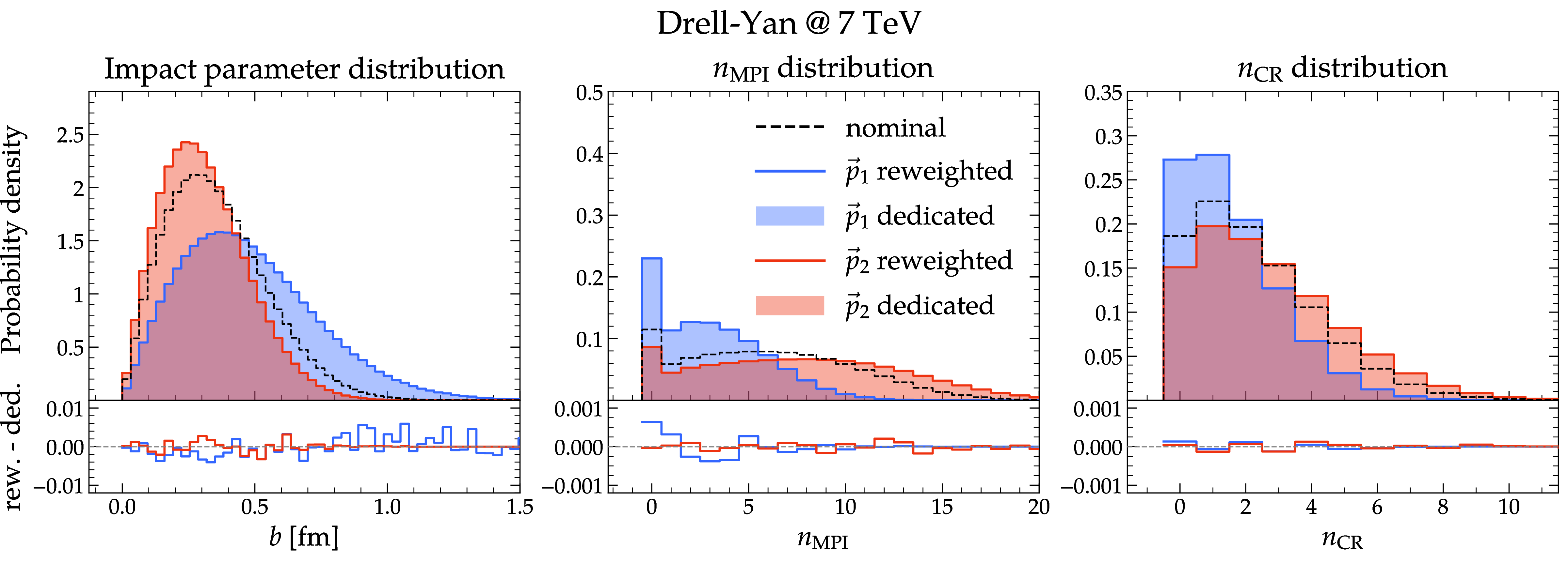
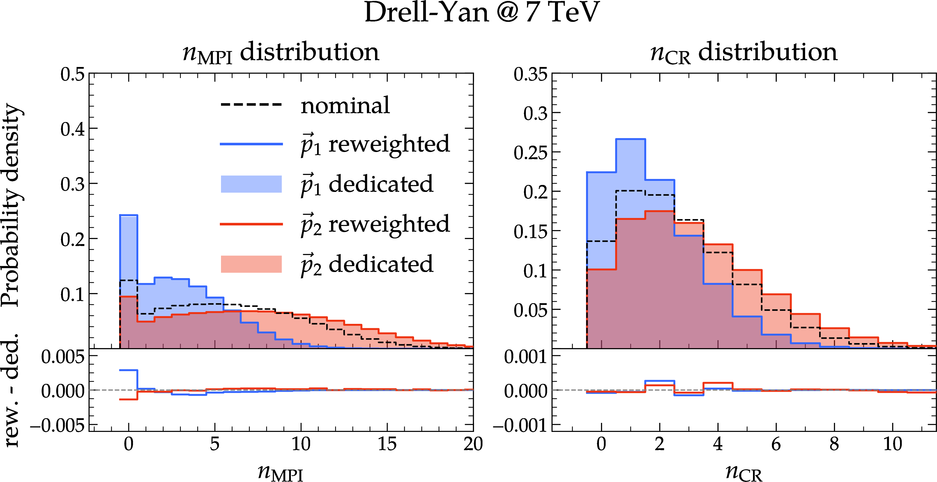
Figure 1 shows closure tests for three intrinsic model observables that systematically validate the individual reweighting components. The first panel probes the probability distribution of the impact-parameter \(b\), testing the geometrical reweighting factor \((w_b)_i\), cf. Eq. (5 ). The second panel examines the MPI multiplicity \(n_{\rm MPI}\), which depends on the full MPI weight \(w_i = (w_b)_i \cdot (w_{\rm Sudakov})_i\) and thus critically tests the reweighting of the Sudakov factor. The third panel validates the CR reweighting through the number of colour reconnections \(n_{\rm CR}\). The parameter variations are specifically designed to demonstrate successful reweighting towards both higher and lower values of each observable (see caption for details). Dedicated samples generated directly for the varied parameter points show excellent agreement with predictions obtained from reweighting the nominal event sample, indicated by the dashed line.
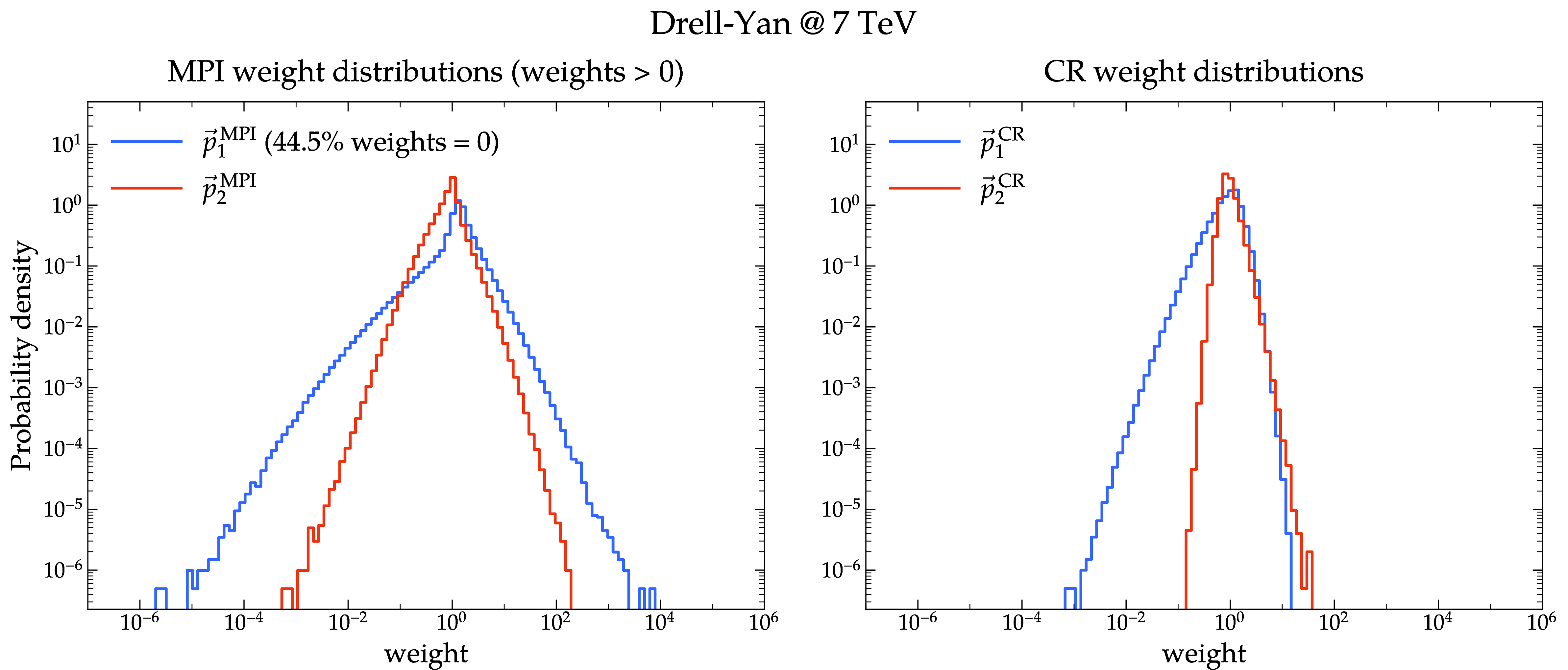
The corresponding distributions of reweighting weights are shown in Figure 2. They remain well-behaved with distributions centred around unity, indicating numerical stability of the reweighting approach. Notably, the first MPI variation (\(\vec{p}^{\rm\:MPI}_1\)) contains an upward variation of \(p_{\perp,\min}^{\rm ref}\) from \(1.0\) to \(1.3~{\rm GeV}\), which produces \(\sim45\%\) zero weights due to the phase-space restriction, cf. Eq. (6 ). Large variations of \(p_{\perp,\min}^{\rm ref}\) thus significantly reduce the effective number of non-zero weights, a limitation that must be considered in practical applications of the reweighting method.
While reweighting intrinsic model variables constitutes a necessary validation of the implementation, closure tests for experimentally relevant physical observables remain essential and are presented in the following section.
3 Tuning methodology and results↩︎
In this section we describe the tools and methods used to tune the S MPI and CR model parameters. As both models have an impact on the final-state hadronic activity, we consider separate tunes for the case of just MPI without the option of CR, and MPI with CR enabled. To facilitate a resource efficient tuning procedure, allowing us to cover a wide range of the parameter space, we build fast surrogate models for the exact generator response to parameter variations using the [15] framework. To train the surrogate model we employ our reweighting technique introduced in Section 2. Following a series of detailed closure tests with dedicated generator runs, we present the physics predictions of our best-tune parameter sets. Finally, we investigate the energy scaling of the dimensionful MPI parameters by tuning against proton–anti-proton collision data at \(\sqrt{s}=1.96\) TeV from the Tevatron and \(13\) TeV LHC data.
3.1 Generator setups and reference data selection↩︎
To constrain the parameters of the S MPI and CR models we employ proton–proton collision data taken by LHC experiments at \(7\) TeV centre-of-mass energy, which accordingly serves as reference scale for energy-dependent model parameters, cf.Eq. 7 . In particular we consider measurements of hadronic observables in Drell–Yan lepton-pair production and pure jet final states accessible through R [42].
Our particle-level event simulations are carried out with a pre-release version of S-3.1 [8] that features our revised CR modelling and the reweighting functionalities for the MPI and CR parameters. We simulate the Drell–Yan and jet-production hard processes at next-to-leading order accuracy in the strong coupling, using tree-level matrix elements from A [43] and C [44], in conjunction with one-loop amplitudes from OpenLoops2 [45] using the C library [46]. The matrix elements are matched to the S dipole shower [35] using the MCNLO formalism [47]. The input value for the strong coupling is set consistently with the employed PDF4LHC21 proton parton-density (PDF) set [48], accessed via LhaPDF [49], to \(\alpha_s(m^2_Z)=0.118\). The PDF and \(\alpha_s\) settings are also used for the secondary scatterings, for which we consider all \(2\to 2\) QCD processes at tree-level accuracy, using \(c_{F,R}=0.5\). The parton-to-hadron transition is modelled with S’s cluster fragmentation [17] using the S-3.0 default parameters determined from tuning to L data [24]. The decays of unstable hadrons are treated by S’s built-in hadron-decay module.
To have sensitivity to the MPI and CR modelling in the simulations we consider measurements that focus in particular on the underlying-event contribution. For the Drell–Yan process we employ an analysis by the ATLAS experiment studying a variety of
charged-particle distributions corresponding to events containing a \(Z^0\)-boson decaying to a pair of electrons or muons [50] (R identifier: ATLAS_2014_I1315949). In addition, we use a similar analysis by CMS [51] considering
muonic final states (CMS_2012_I1107658). Both analyses study charged-particle multiplicities and transverse momenta in regions of azimuthal angle defined with respect to the \(Z^0\)-boson direction,
differential in the di-lepton transverse momentum. For pure jet production we consider two dedicated underlying-event analyses, one from ATLAS [52] (ATLAS_2014_I1298811) and one from CMS [32] (CMS_2011_I916908). Both provide
measurements of charged-particle multiplicities and momentum spectra in azimuthal regions transverse to the leading (track-)jet in the event. Furthermore, we consider a jet-fragmentation-function measurement from ATLAS [53] (ATLAS_2011_I929691), a measurement of transverse event-shape variables from CMS [54] (CMS_2011_I886332), and an energy-flow measurement at large rapidities in dijet events by CMS [55] (CMS_2011_I930319).
3.2 Tuning methodology↩︎
To explore the physics-model parameter space we employ the [15] tuning tool. For all bins of the considered observable histograms constructs a multivariate rational surrogate model \(R(\vec{p})=P(\vec{p})/Q(\vec{p})\) that aims to capture the simulator response on variations of the model parameters \(\vec{p}\). For the tuning problem at hand we found a satisfying approximation quality for a simple polynomial function, i.e.\(P(\vec{p})\) of degree five and \(Q(\vec{p})\) of degree zero. The statistical errors of the MC predictions are accounted for by constructing additional surrogate models of the same form for the uncertainties in each histogram bin.
We consider two scenarios for the tuning:
MPI-CRoff: The option to probabilistically rearrange the colour assignments of partons is disabled, the tuning comprises the four MPI model parameters listed in Table 3, where we also quote the initial parameter ranges.
MPI-CRon: CR is enabled and the tuning furthermore includes the \(\eta_Q\) parameter, cf. Table 3 for the considered parameter ranges.
| value/tune range | ||
| Parameter | MPI-CRoff | MPI-CRon |
| \(R_1\,[\text{fm}]\) | \([0.75,0.95]\) | |
| \(R_2\,[\text{fm}]\) | \(1.0\) | |
| \(\alpha_1\) | \([0.30,0.70]\) | |
| \(\sigma_{\rm ND}^{\rm norm}\) | \([0.30,0.70]\) | |
| \(p_{\perp,0}^{\rm ref}\,[\text{GeV}]\) | \(2.05\) | |
| \(p_{\perp,\min}^{\rm ref}\,[\text{GeV}]\) | \([1.00,1.30]\) | |
| \(c_R\) | \(0.5\) | |
| \(c_F\) | \(0.5\) | |
| \(\eta_Q\) | – | \([0.35,0.65]\) |
| \(R\) | – | \(1/9\) |
| \(Q_0\,[\text{GeV}]\) | – | \(1.0\) |
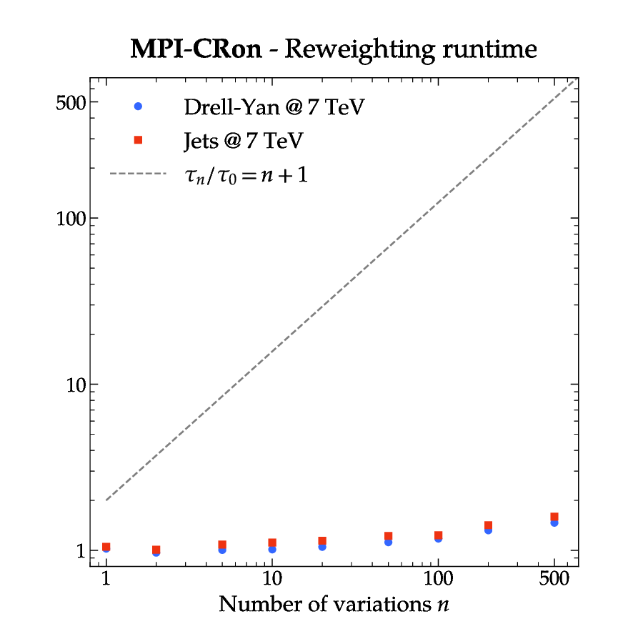
To cover the available model space, we generate \(500\) random parameter configurations uniformly distributed over the four- and five-dimensional parameter hyperrectangle, respectively. Instead of performing dedicated S simulations for each of these points, we employ the reweighting method described in Sections 2.1 and 2.2. As the nominal parameter set, we use \[\vec{p}_0 = \left(R_1=0.85\,\text{fm}, \alpha_1=0.5, \sigma_{\rm ND}^{\rm norm}=0.5, p_{\perp,\min}^{\rm ref}=1.0\,\text{GeV}\right)\,,\] which is extended by the CR parameter \(\eta_Q=0.5\) 6 for the MPI-CRon scenario. Accordingly, from these nominal samples we produce predictions for the \(500\) parameter points, respectively, through reweighting. Compared to the time needed to generate \(500\) dedicated samples, this approach reduces the compute time by about a factor \(250\). We briefly discuss the scaling behaviour of the reweighting method in Appendix 6, see in particular Fig. 17.
As several analyses targeting different processes enter the tune simultaneously, they can contribute very differently to the objective function. To avoid any single process dominating the goodness-of-fit (GOF), and thereby biasing the resulting parameters, we rescale the per-observable weights of each process group (Drell–Yan/jets) by a common factor such that all groups contribute comparably. These factors are fixed from the minimal GOF of separate fits to the individual processes.
Before performing the parameter optimisation, we validate the reweighting procedure by means of dedicated closure tests. For each model parameter individually, we compare predictions obtained by reweighting the nominal sample \(\vec{p}_0\) against dedicated S runs generated directly for the varied parameter point, while keeping all other parameters fixed at their nominal values. The parameter variations are chosen to cover the respective tuning ranges listed in Table 3, probing the boundaries of the parameter hyperrectangle along each individual axis7.
Figures 3 and 4 show representative closure-test results on selected observables from the Drell–Yan and dijet processes, respectively, for the MPI-CRon scenario; the variations of the four MPI parameters are common to both the MPI-CRoff and MPI-CRon setups, while the \(\eta_Q\) variation (orange) enters only the latter. The largest impact on the observables is observed for the \(\sigma_{\text{ND}}^{\rm norm}\) variations. Notably, for the charged-particle multiplicity in Drell–Yan production the impact of variations of the CR parameter \(\eta_Q\) is of similar strength as that of the matter-profile parameters. We again remark that the \(p_{\perp,\min}^{\rm ref}\) parameter can only be varied to larger values, i.e.here from \(1.0\,\text{GeV}\) to \(1.3\,\text{GeV}\). In all variations the reweighted predictions are in very good agreement with the dedicated generator runs across the full distributions, confirming that the reweighting procedure accurately captures the generator response to individual parameter variations over the full tuning ranges considered.
![Figure 3: The number of charged particles N_{\rm ch} in the toward region in Drell–Yan events at \sqrt{s}=7\,\text{TeV}, with independent variations of the MPI parameters p_{\perp,\min}^{\rm ref} (red), \sigma_{\rm ND}^{\rm norm} (blue) and \rho(R_1, \alpha_1) (green) and the CR parameter \eta_Q (orange). The left panel shows the variations obtained from the reweighting procedure, with the nominal parameter set \vec{p}_0 described in Section 3. The panels on the right compare the reweighting-based variations to those obtained from dedicated generator runs at the varied parameter points. Parameter values are given in the notation [nominal, variation 1, (variation 2)].](/article/2606.24702/plots/CMS_2012_I1107658_d13-x01-y01_CR.png "fig:")
![Figure 4: Sum of transverse momenta of charged particles in the transverse region in inclusive jet events at \sqrt{s}=7\,\text{TeV}, with independent variations of the MPI parameters p_{\perp,\min}^{\rm ref} (red), \sigma_{\rm ND}^{\rm norm} (blue) and \rho(R_1, \alpha_1) (green) and the CR parameter \eta_Q (orange). The left panel shows the variations obtained from the reweighting procedure, with the nominal parameter set \vec{p}_0 described in Section 3. The panels on the right compare the reweighting-based variations to those obtained from dedicated generator runs at the varied parameter points. Parameter values are given in the notation [nominal, variation 1, (variation 2)].](/article/2606.24702/plots/ATLAS_2014_I1298811_d16-x01-y01_CR.png "fig:")
To quantify the statistical dilution due to reweighting, introducing event-weight factors \(w^{(i)}\) for parameter variation \(\vec{p}_i\), we consider the effective sample size
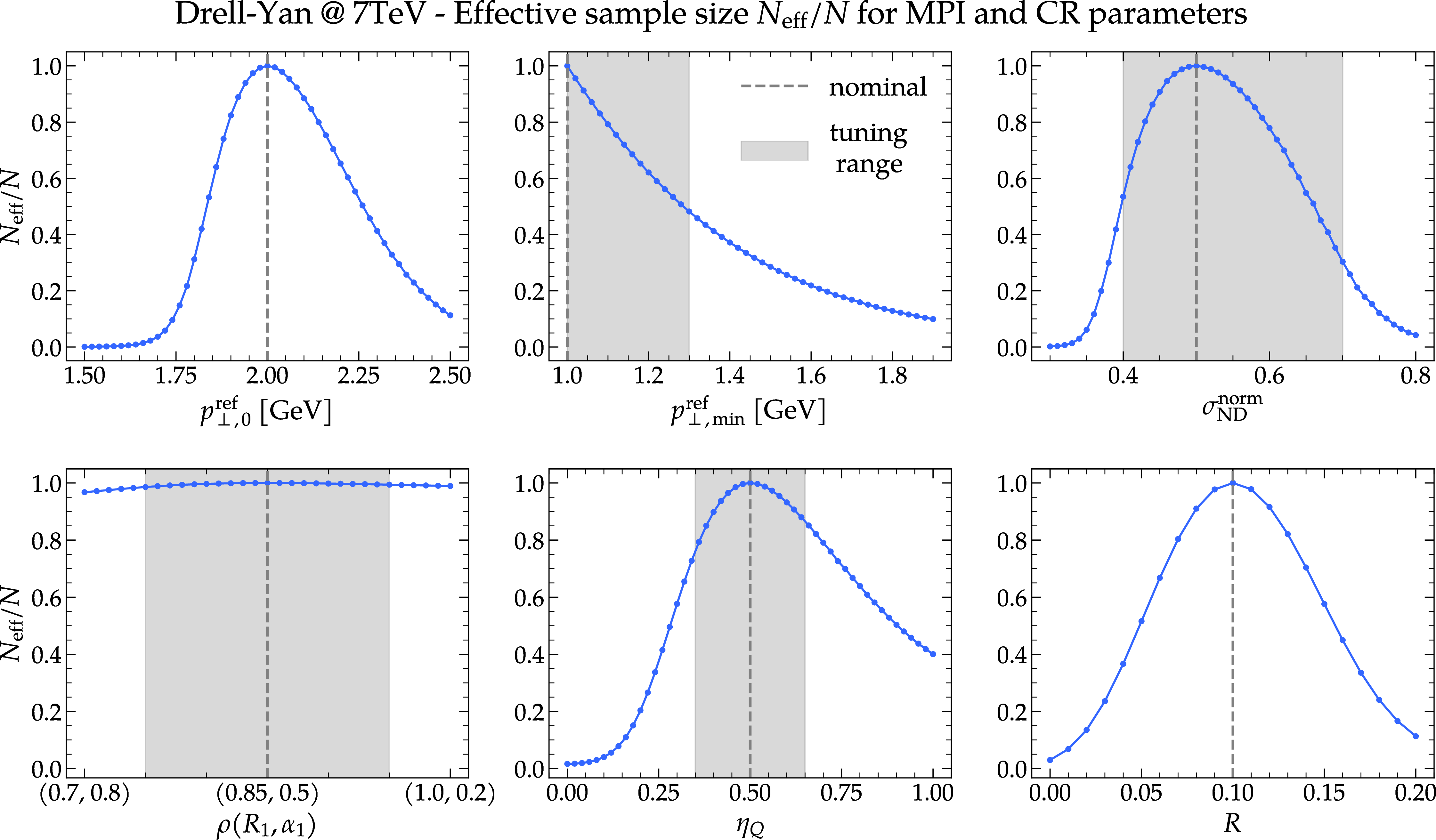
\[N^{(i)}_{\rm eff} = \frac{\left(\sum_{j=1}^N w^{(i)}_j\right)^2}{\sum_{j=1}^N \left(w^{(i)}_j\right)^2}\,, \label{eq:neff}\tag{9}\] where \(N\) is the total number of nominal events generated for \(\vec{p}_0\), while \(w^{(0)}_j=1\) for all \(j\) and thus \(N^{(0)}_{\rm eff}=N\). Accordingly, this quantity measures the reduction in statistical power due to broadly distributed or highly non-uniform event weights, and therefore provides a convenient measure of the stability of the reweighting procedure. Figure 5 shows the effective sample size relative to the nominal sample, i.e.\(N^{(i)}_{\rm eff}/N\), for the same single-parameter variations used in the closure tests above, including the combined \(\rho(R_1, \alpha_1)\) variation.
Moving away from the nominal set the effective sample size drops quite quickly. A notable exception are the matter-profile parameters, which result in rather small weight variations. We here also indicate the parameter ranges considered in the tuning. Also for the parameters inducing rather significant reweighting factors, i.e.\(p_{\perp,\min}^{\rm ref}\) and \(\sigma_{\rm ND}^{\rm norm}\), even at the boundaries of the tuning range the effective sample size is still \({\cal{O}}(N/2)\). These dilution effects need to be taken into account when setting up the tuning process. First, sufficiently large event samples need to be considered such that such a reduction in statistical power does not invalidate their usability for comparison with measurement data of a given systematic and statistical uncertainty. Second, if the drop in the effective sample size appears to be too large or wider parameter variations are considered, additional nominal samples can be generated and reweighted accordingly.
3.3 Underlying Event tunes for S↩︎
Having validated our novel reweighting method and with our corresponding tuning methodology established we now move to the discussion of our resulting tunes of the S MPI and CR models. We consider two situations, namely MPI with CR disabled and with CR switched on. The best-tune parameter sets we obtain for the MPI-CRoff and MPI-CRon scenarios are: \[\begin{align} \text{\boldsymbol{MPI-CRoff:}} \quad \vec{p}^{\,*} &= \left(R_1=0.93\,\text{fm},\;\alpha_1=0.32,\;\sigma_{\rm ND}^{\rm norm}=0.50,\; p_{\perp,\min}^{\rm ref}=1.14\,\text{GeV}\right), \nonumber\\ \text{\boldsymbol{MPI-CRon:}} \quad \vec{p}^{\,*} &= \left(R_1=0.85\,\text{fm},\;\alpha_1=0.65,\;\sigma_{\rm ND}^{\rm norm}=0.44,\; p_{\perp,\min}^{\rm ref}=1.10\,\text{GeV},\;\eta_Q=0.63\right). \nonumber \end{align}\] Figures 6 and [fig:results95Jets95CR95off] show a representative selection of predictions at \(\vec{p}^{\,*}\) for the MPI-CRoff tune, comparing to the ATLAS Drell–Yan underlying-event measurement [50] and the ATLAS underlying-event analysis in jet production [53], respectively. Selected MPI-CRon predictions are displayed in Figures 7 and [fig:results95Jets95CR95on]. In each figure we show two theory predictions at \(\vec{p}^{\,*}\): one obtained from a dedicated S run with the best-tune parameters, and one obtained by reweighting the nominal sample \(\vec{p}_0\) to \(\vec{p}^{\,*}\). The agreement between the two demonstrates that the reweighting method is capable of faithfully reproducing simultaneous multi-parameter variations across all considered observables, without the need for additional generator runs. The Apprentice surrogate prediction at \(\vec{p}^{\,*}\) is overlaid, showing that the employed polynomial approximation accurately captures the full generator response at the best-tune point.
![Figure 6: Results for the best-tune parameter set \vec{p}^{\,*} for the MPI-CRoff scenario, compared to the ATLAS Drell–Yan underlying-event measurement [50].](/article/2606.24702/_pdflatex/uxgrzfde.png "fig:")
![Figure 7: Results for the best-tune parameter set \vec{p}^{\,*} for the MPI-CRon scenario, compared to the ATLAS Drell–Yan underlying-event measurement [50].](/article/2606.24702/_pdflatex/tziekuha.png "fig:")
The effective sample size ratios, cf.Eq. 9 , and the average reweighting weights for all four runs are summarised in Table 4. These quantities provide a compact measure of the statistical efficiency and demonstrate that the weights remain well behaved, including for the combined MPI and CR variations. The full distributions of the reweighting weights are shown in the Appendix 6 in Figure 18.
| Sample | \(N_{\rm eff}/N\) | \(\langle w\rangle\) |
|---|---|---|
| MPI-CRoff - Drell–Yan | \(0.72\) | \(1.000\) |
| MPI-CRon - Drell–Yan | \(0.58\) | \(0.999\) |
| MPI-CRoff - Jets | \(0.72\) | \(1.003\) |
| MPI-CRon - Jets | \(0.56\) | \(0.994\) |
| \(\chi^2/{\rm ndf}\) | ndf | ||
| Process/Analysis | MPI-CRoff | MPI-CRon | |
| Drell–Yan (cum.) | \(34.0\) | \(16.1\) | \(2573\) |
| ATLAS_2014_I1315949 | \(32.4\) | \(14.7\) | \(2123\) |
| CMS_2012_I1107658 | \(41.7\) | \(22.6\) | \(450\) |
| Jets (cum.) | \(2.5\) | \(2.0\) | \(1690\) |
| ATLAS_2014_I1298811 | \(2.7\) | \(2.1\) | \(1035\) |
| ATLAS_2011_I929691 | \(1.6\) | \(1.4\) | \(409\) |
| CMS_2011_I916908 | \(3.6\) | \(2.1\) | \(163\) |
| CMS_2011_I886332 | \(3.1\) | \(4.0\) | \(78\) |
| CMS_2011_I930319 | \(1.1\) | \(1.2\) | \(5\) |
A quantitative summary of the description quality at the best-tune points is provided in Table 5, with per-observable \(\chi^2/{\rm ndf}\) values shown in Figure 8 for the two considered Drell–Yan analyses (analogous plots for the four jet-production analyses with more than one histogram appear in Appendix 6). The MPI-CRon tune yields a better overall agreement with the data than MPI-CRoff, both in the Drell–Yan and jet sectors, but in particular in the former, where the \(\chi^2/{\rm ndf}\) values are effectively halved. This establishes the CR-enabled scenario as the preferred tune. The \(\chi^2/\mathrm{ndf}\) values obtained here are consistent with those from a conventional tune based on dedicated generator runs at each parameter point8, confirming that the reweighting-based approach is a reliable and computationally efficient alternative to a tune based on dedicated simulation runs.
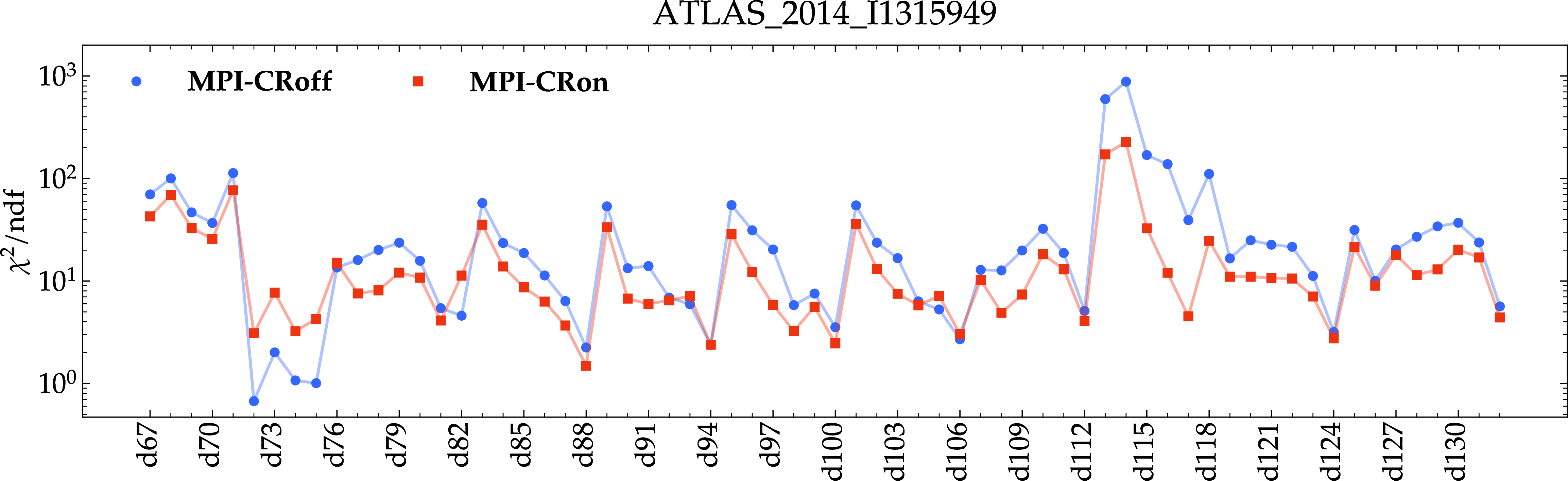
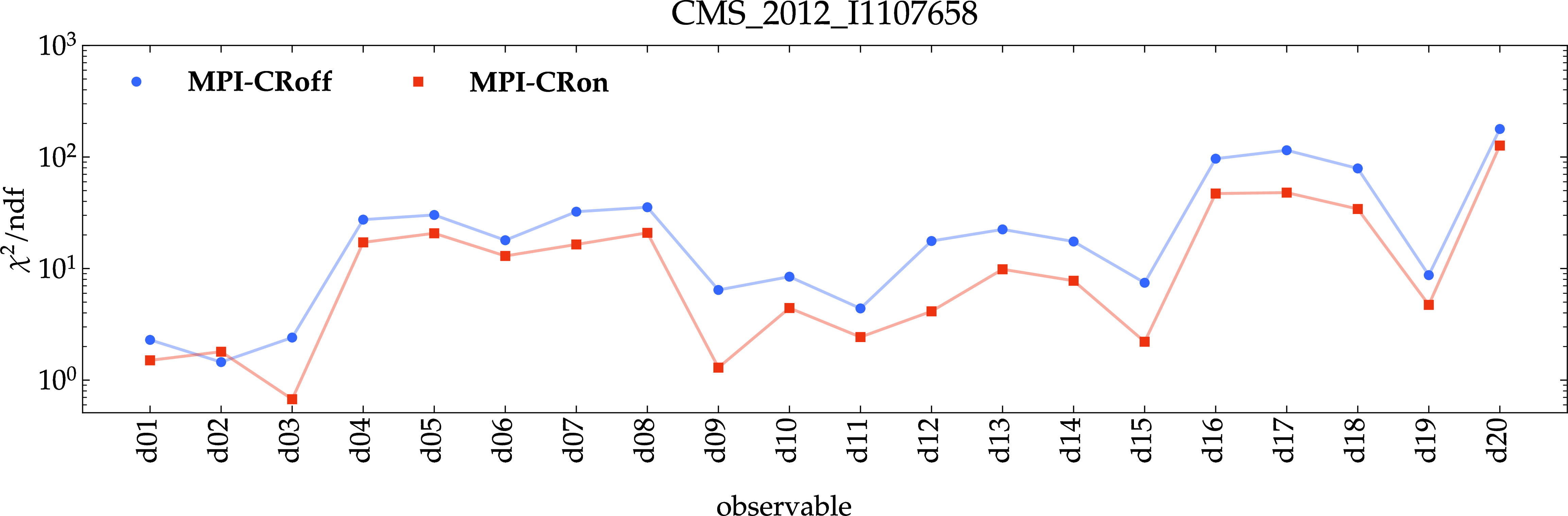
Figure 8: The \(\chi^2/{\rm ndf}\) values per observable for all Drell–Yan analyses considered in the MPI-CRoff and MPI-CRon tunes..
To make the impact of colour reconnection on the physical distributions explicit, Figure 9 directly compares the MPI-CRoff and MPI-CRon best-tune predictions with data for a representative set of Drell–Yan and jet observables used in the tune. Colour reconnection, which rearranges the colour flow prior to cluster formation and thereby increases the average transverse momentum of the produced hadrons at a given multiplicity, improves the description of observables that correlate \(\langle p_\perp\rangle\) with the charged-particle multiplicity (right column), which is largely driven by the underlying event. Here the tune without CR undershoots the data and yields too weak a rise of \(\langle p_\perp\rangle\) with \(N_{\rm ch}\), whereas the MPI-CRon tune recovers the measured trend without degrading the already good description of the observables in the left column. This improvement is the main source of the lower \(\chi^2/{\rm ndf}\) obtained for CR-enabled-scenario in Table 5.
![Figure 9: Direct comparison of the MPI-CRoff (blue) and MPI-CRon (red) best-tune predictions with data, for representative underlying-event observables inDrell–Yan (top) and jet (bottom) production at \sqrt{s}=7\,\text{TeV}. Left: the transverse-region charged-particle density versus the di-muon transverse momentum [51]and the transverse-region charged p_\perp sum [32]. Right: the mean charged-particle transverse momentum as a function of multiplicity in the transverse region,from the ATLAS Drell–Yan [50] and ATLAS jet [52] measurements.](/article/2606.24702/_pdflatex/bqgimdcu.png "fig:")
3.4 Energy extrapolation↩︎
| \(\chi^2/{\rm ndf}\) | ndf | |
| Analysis | MPI-CRon | |
| ATLAS_2019_I1736531 | \(28.6\) | \(14927\) |
| CDF_2015_I1388868 | \(16.3\) | \(120\) |
Having established best-tune parameter sets at a reference scale \(s_\text{ref}\), here \(\sqrt{s_\text{ref}}=7\,\text{TeV}\), we still need to determine the scaling parameter \(\eta\) that according to Eq. 7 determines the values of the dimensionful MPI parameters at an alternative scale. To this end, we perform a dedicated one-parameter Apprentice tune of \(\eta\) using underlying-event measurements at two different centre-of-mass energies: an ATLAS Drell–Yan underlying-event analysis at \(\sqrt{s}=13\,\text{TeV}\) [56] (ATLAS_2019_I1736531) and a CDF track-based underlying-event study in
\(p\bar{p}\) collisions at \(\sqrt{s}=1.96\,\text{TeV}\) [57]
(CDF_2015_I1388868).
In both cases we employ the MPI-CRon tune from the previous section as a baseline and use the reweighting procedure to scan \(\eta\) in the range \([0.0, 0.08]\), while keeping all other parameters fixed at their best-tune values. Note, variations of \(\eta\) are constrained by the same phase-space limitation as \(p_{\perp,\min}^{\rm ref}\), i.e.only variations in one direction are possible. The direction thereby depends on whether the target collision energy \(\sqrt{s}\) exceeds or falls below the reference scale. Consequently, for the \(13\;\text{TeV}\) LHC runs we use \(\eta=0\) as nominal value, for the Tevatron setup instead \(\eta=0.08\) is used as baseline.
For the tuning grid we consider \(18\) uniformly spaced \(\eta\) values, and the surrogate model is constructed as a simple polynomial function of degree three. A representative validation of the energy extrapolation across the entire tuning range is shown in Figures 10 and 11 for the LHC and the Tevatron analysis, respectively. In both cases the reweighted predictions for different values of \(\eta\) are in very good agreement with the dedicated S runs across the full distributions. The effective sample size for the reweighted samples is shown in Figure 12.
![Figure 10: Closure test for the MPI energy-extrapolation parameter \eta using the ATLAS underlying-event measurement in inclusive Z-boson production at \sqrt{s}=13\,\text{TeV} [56]. The left panel shows the variations obtained from the reweighting procedure of \eta for the MPI-CRon best-tune parameter set. The panels on the right compare the reweighting-based variations to those obtained from dedicated generator runs for the corresponding \eta values.](/article/2606.24702/plots/ATLAS_2019_I1736531_d446-x01-y01_CR.png "fig:")
![Figure 11: Closure test for the MPI energy-extrapolation parameter \eta using the CDF underlying-event measurement in p\bar{p} collisions at \sqrt{s}=1.96\,\text{TeV} [57]. The left panel shows the variations obtained from the reweighting procedure of \eta for the MPI-CRon best-tune parameter set. The panels on the right compare the reweighting-based variations to those obtained from dedicated generator runs for the corresponding \eta values.](/article/2606.24702/plots/CDF_2015_I1388868_d05-x01-y01_CR.png "fig:")

The two reference measurements are combined following the same prescription as for the 7 TeV tune (cf.Section 3.2): the per-observable weights of the ATLAS (13 TeV) and CDF (1.96 TeV) data sets are rescaled such that the extracted value of \(\eta\) is not driven by a single energy point. From the combined description we obtain an optimal value of \(\eta^* = 0.026\) for the energy-extrapolation exponent. The \(\chi^2/{\rm ndf}\) values for both analyses at \(\eta^*\) are shown in Table 6.
We close the discussion of the energy-scaling of MPI parameters by showing two exemplary observable distributions for the MPI-CRon best-tune parameter set supplemented by \(\eta^*=0.026\) in Fig. 13. In the left panel we show the differential distribution of the charged-particle density in the trans-min region with respect to the \(Z\) boson, comparing to data from the ATLAS experiment [56]. The right panel, instead, shows for the same region, but defined with respect to the leading charged particle, the charged-particle density differential in the leading charged particle transverse momentum, comparing to data from CDF [57]. For both distributions S provides a good description of the data, although there is certainly space for improvement. Furthermore, with the advent of the high-luminosity LHC and more analyses at \(13\) and \(13.6\,\text{TeV}\) becoming available, a dedicated tune at these higher energies, without having to rely on the energy-scaling hypothesis, is well motivated.
![Figure 13: Best-tune MPI-CRon predictions supplemented with the energy-extrapolation exponent \eta^*=0.026 (red), compared with data.Left: the trans-min charged-particle density in the low-thrust region for 10<p_T^Z<20\,\text{GeV}, from the ATLAS inclusiveZ-boson underlying-event measurement at \sqrt{s}=13\,\text{TeV} [56]. Right: the trans-min charged-particle density as a function of theleading-particle transverse momentum p_T^{\rm max}, from the CDF underlying-event measurement in proton–anti-protoncollisions at \sqrt{s}=1.96\,\text{TeV} [57].](/article/2606.24702/_pdflatex/awyrfdji.png "fig:")
4 Conclusions and Outlook↩︎
In this paper we have presented the first implementation and careful validation of an on-the-fly reweighting algorithm to account for model-parameter variations in MPI and CR simulations with the S event-generator framework. In a single run, using a nominal set of parameters, our method evaluates in-situ event-wise variational weights corresponding to alternative points in model-parameter space. We have performed detailed closure tests, both for model-internal variables and actual physical observables, proving that the corresponding predictions agree with the outcome of dedicated simulator runs. While in principle parameters can be varied largely at will, there are inherent limitations. Certain parameters, whose settings restrict the phase space, can only be varied unidirectionally. For the case of MPI this applies in particular to the transverse-momentum cutoff of the secondary scatterings, i.e.\(p_{\perp,\min}^{\rm ref}\), which, with respect to the nominal value, can only be reweighted for upward variations. The introduction of additional event weights leads to a statistical dilution of the variational samples with respect to the nominal case, an effect that can be measured by the Kish effective sample size. The reduced statistical power for parameter points significantly away from the nominal set can potentially limit the usability of the corresponding predictions. This limitation, however, can easily be counteracted by the introduction of additional nominal runs, and, as far as computationally feasible, by increasing the statistics of the nominal sample.
The benefits of the reweighting technique are manifold: based on a single (or potentially a few) simulator runs, it allows us to produce a significant number of alternative predictions with rather little computational overhead, paying off for two variations already. The computational needs for sample production are massively reduced. The same holds for storage and post-processing, e.g.in an analysis or when invoking a detector simulation, where only a single sample, supplemented by alternative event weights, needs to be processed. This qualifies our method for example for parameter-sensitivity studies, model-calibration and tuning tasks, as well as uncertainty quantification at drastically reduced computational cost compared to the current standard procedures.
As a first illustrative use case we have applied the method in the combined tuning of the S MPI and CR models. To this end, we considered underlying-event analyses in proton–proton collisions at \(\sqrt{s}=7\,\text{TeV}\), and produced corresponding generator predictions for \(500\) random samples from the \(4\)-dimensional (MPI-CRoff) and \(5\)-dimensional (MPI-CRon) parameter spaces via reweighting from a single nominal run, respectively. These predictions are then used to train polynomial surrogate models using the Apprentice package. Through comparison with data we find best-tune parameter sets that provide an improved description of the considered Drell–Yan and jet-production data. We find that the experimental data favours the inclusion of colour reconnections in the simulation.
To fix the scaling of dimensionful model parameters with the collision energy we furthermore performed a simple one-parameter tune of the relevant scaling exponent, using LHC \(pp\) data at \(13\,\text{TeV}\) and \(p\bar{p}\) data at \(1.96\,\text{TeV}\) from the Tevatron. For both energies, the corresponding predictions for \(18\) parameter points have been obtained via reweighting from a nominal value, respectively. With the obtained optimal parameter, the rescaled versions of our best-tune MPI-CRon parameter set extracted at \(\sqrt{s}=7\,\text{TeV}\) provide a satisfactory description of the considered data.
Our reweighting method for MPI and CR simulations closes a significant gap in the capabilities of modern Monte Carlo event generators to efficiently provide predictions for alternative non-perturbative model parameters. While parameter calibration, i.e.generator tuning, is an attractive application of such a reweighting technique, we envisage that in practice it has the largest impact on parameter-sensitivity studies and, in particular, the quantification of non-perturbative uncertainties. In particular for the recently presented History Matching calibration method [16] reweighting is a natural fit, as samples from a non-implausible parameter space can be used to reflect the inherent parametric uncertainties of a complex model. To this end, we plan to transfer our approach to S’s cluster-fragmentation model [17], [58], as well as minimum-bias simulations, and the generation of the intrinsic transverse momenta. Ultimately, we aim to provide support for the reweighting of all non-perturbative parameters in S. The method presented here will pave the way to a new approach to robustly and systematically assess parametric uncertainties of non-perturbative models, and will be essential for the upcoming high-luminosity era of LHC operations.
Acknowledgements↩︎
S.S.is grateful for financial support from the German Federal Ministry of Research, Technology and Space (projects 05D23MG1 and 05H24MGA). This material is based upon work supported by Fermi Forward Discovery Group, LLC under Contract No. 89243024CSC000002 with the U.S. Department of Energy, Office of Science, Office of High Energy Physics. The work of M.K.was supported by the U.S. Department of Energy, Office of Science, Office of Advanced Scientific Computing Research, Scientific Discovery through Advanced Computing (SciDAC-5) program, grant “NeuCol”. F.K.acknowledges funding by STFC under grant agreement ST/P006744/1.
5 Configuring MPI and CR Variations↩︎
The reweighting functionality for the S MPI and CR models can be enabled by specifying lists of parameter values directly in the run card9, instead of single values. The first element in each list corresponds to the nominal value (used for the main S event generation), while the remaining entries define the parameter variations for which additional weights will be computed.
As an example, the run card setting
SIGMA_ND_NORM: [0.5, 0.4, 0.6]will use \(0.5\) as nominal value for the \(\sigma_{\rm ND}^{\rm norm}\) parameter and additionally compute reweighted event weights corresponding to the alternative values \(0.4\) and \(0.6\).
When multiple parameters are varied simultaneously, the variations are matched by their position in the respective lists. That is, the first variation entry of each parameter forms one variation set, the second entries forms the next set, and so on. For example,
    SIGMA_ND_NORM: [0.5, 0.4, 0.6]
    PT_Min(ref): [1.0, 1.2, 1.4]
will produce a S run with the nominal parameter set \[\vec{p}_0=(\texttt{SIGMA\_ND\_NORM},\texttt{PT\_Min(ref)})=(0.5,1.0)\,,\] and generate variation weights for \[\vec{p}_1=(0.4,1.2),\quad\vec{p}_2=(0.6,1.4)\,.\] If the number of variation entries differs between parameters, missing values are automatically filled with the corresponding nominal value. For instance,
    SIGMA_ND_NORM: [0.5, 0.4, 0.6]
    PT_Min(ref): [1.0, 1.2]
results in the two variations \[\vec{p}_1=(0.4,1.2),\quad\vec{p}_2=(0.6,1.0)\,.\] The same syntax applies to all parameters controlling the MPI and CR models listed in Table 1 and Table 2. Mixed variations of both parameter groups are also supported, and S will combine the respective weights accordingly. For example
    AMISIC:
      SIGMA_ND_NORM: [0.5, 0.4, 0.6]

    COLOUR_RECONNECTIONS:
      ETA_Q: [0.5, 0.4, 0.6]
will produce a S run with the nominal parameter set \[\vec{p}_0=(\texttt{SIGMA\_ND\_NORM},\texttt{ETA\_Q})=(0.5,0.5)\,,\] and the variations \[\vec{p}_1=(0.4,0.4),\quad\vec{p}_2=(0.6,0.6)\,.\] The reweighting outputs, i.e.the variational event weights, are available both in the HepMC [41] event record and through the S internal Rivet interface. The variation weights are labelled as SoftPhysics.v1,
SoftPhysics.v2, etc., where v1 corresponds to the first specified variation, i.e.\(\vec{p}_1\).
6 Auxiliary material↩︎
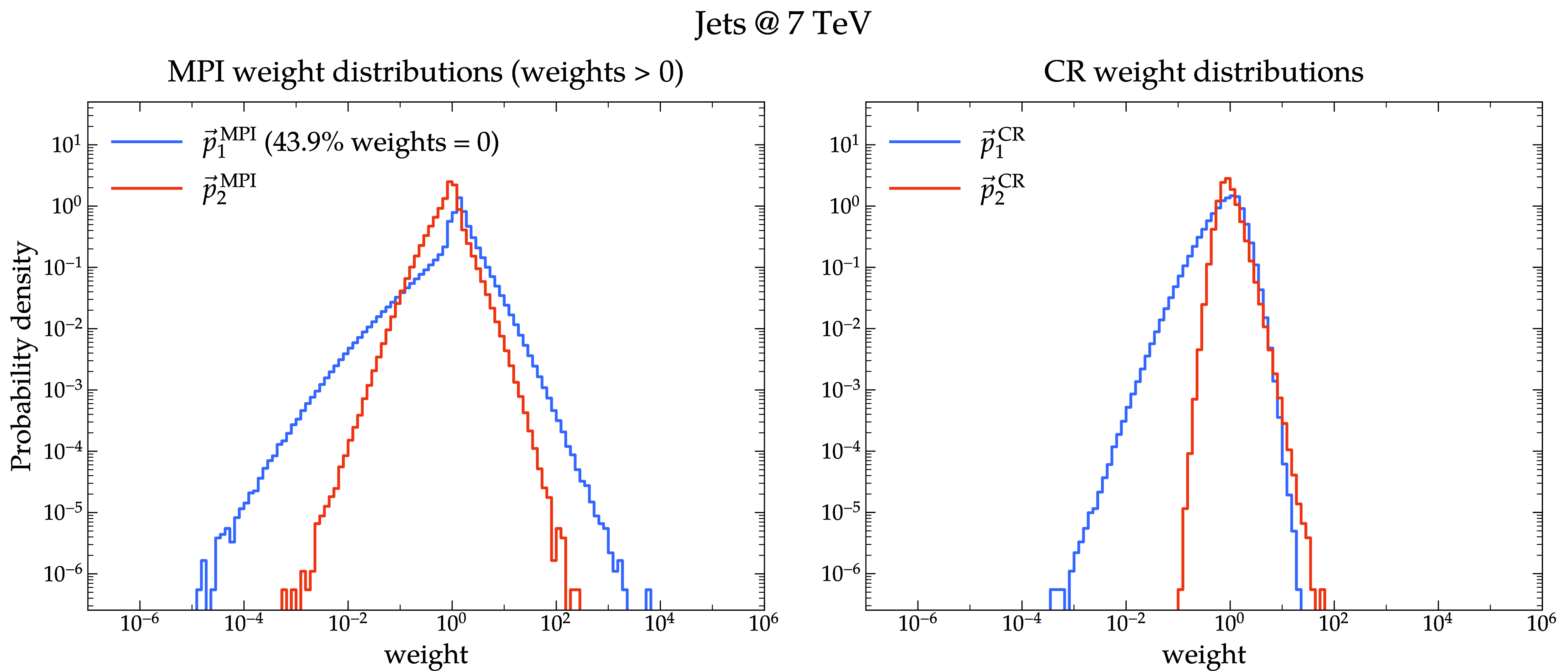
![Figure 18: Distribution of the total reweighting event weights obtained from the best-tune parameter runs (Figures 6-[fig:results95Jets95CR95on]) for MPI-CRoff (left) and MPI-CRon (right) tunes. The distributions are shown for the Drell–Yan and jet samples, respectively.](/article/2606.24702/_pdflatex/knolxszr.png "fig:")
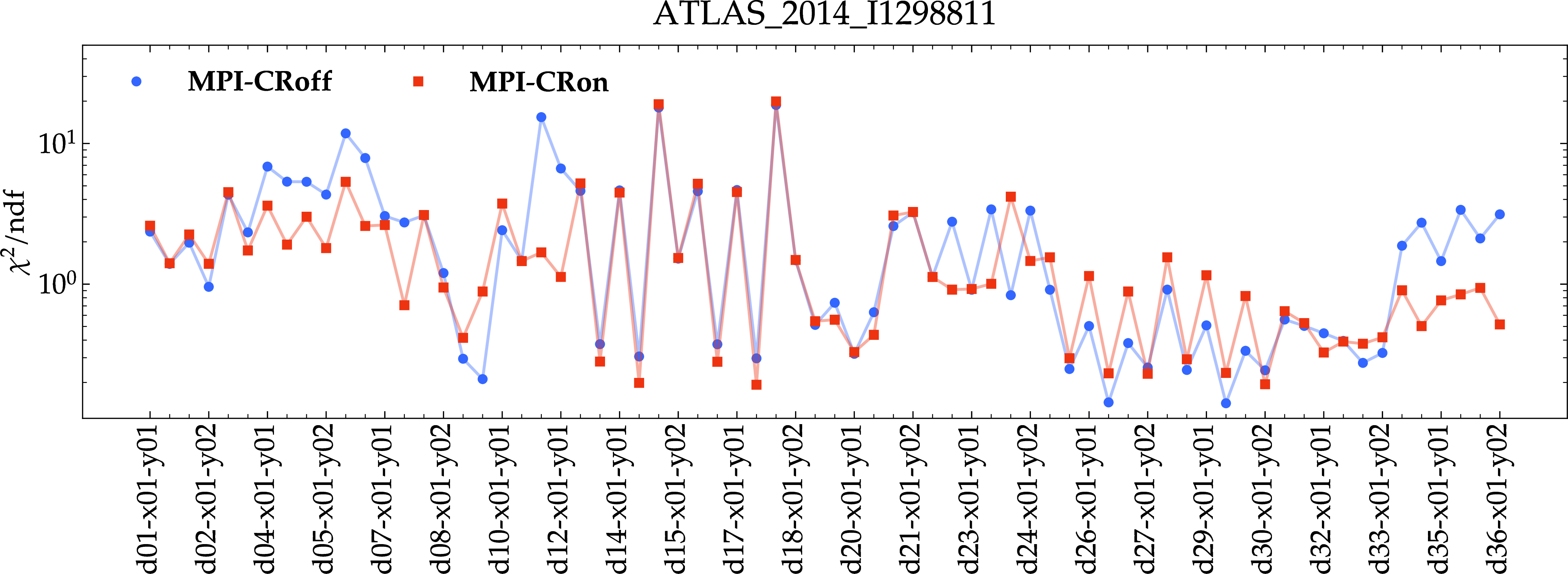
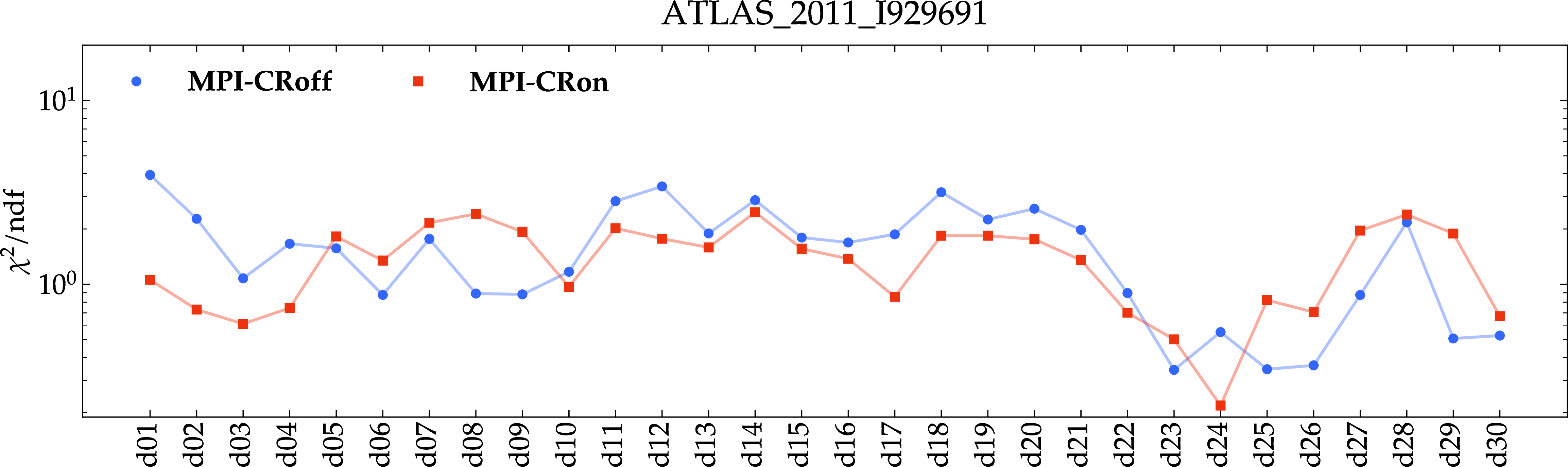
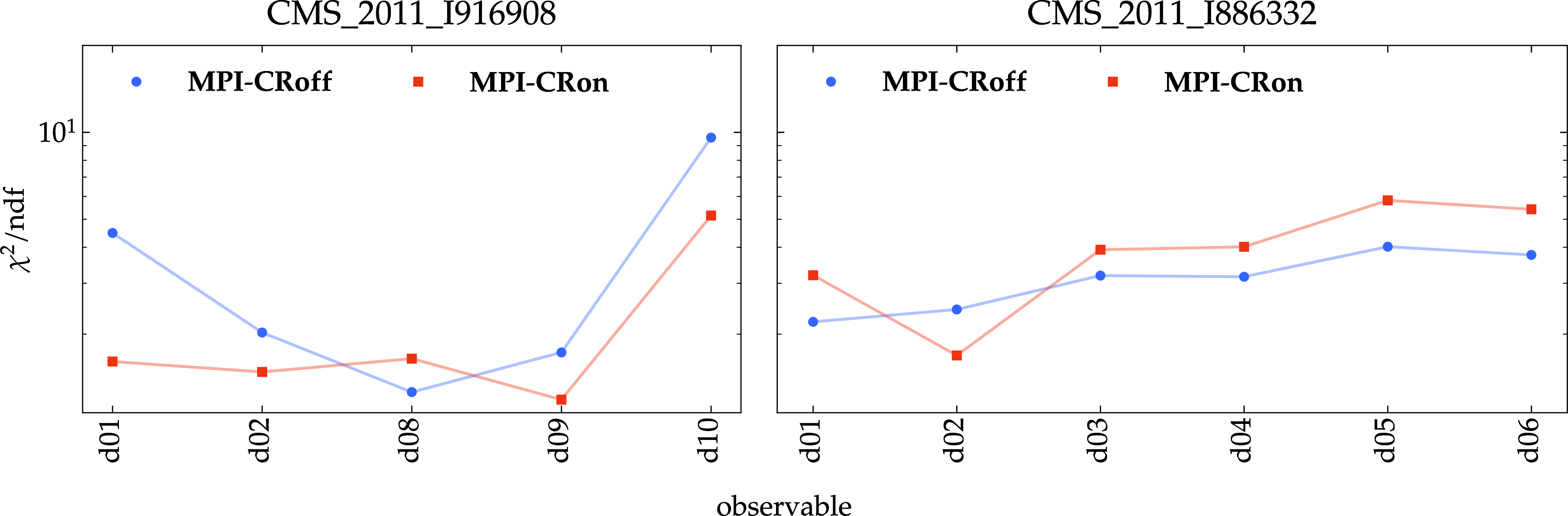
Figure 19: \(\chi^2/{\rm ndf}\) values per observable for all jet analyses considered in the MPI-CRoff and MPI-CRon tunes, excluding CMS_2011_S9215166, which
contains only a single valid observable..
References↩︎
The HM method identifies regions of parameter space not excluded by the considered calibration data, rather than isolating a single best-fit point, as is the case for traditional approaches. This is achieved through a consecutive compression of the parameter-space volume based on a suitable implausibility measure. This yields a more realistic picture of parameter degeneracies and correlated uncertainties, which are represented by space-filling samples from the remaining non-implausible parameter-space volume. In Ref. [16] the HM approach was applied to the hadronisation models accessible through S, namely its built-in cluster fragmentation Ahadic [17], and the Lund-string fragmentation [18] through an interface to P 8 [5].↩︎
To be precise, typically not the strict ’t Hooft limit [34] (\(N_c\to \infty\) with \(\alpha_sN_c=\text{const.}\)) is used. Instead, formally subleading \(g\to q\bar{q}\) splittings are included and the QCD Casimirs appearing in the splitting functions remain at their proper \(N_c=3\) values, i.e.\(C_A=3\) and \(C_F=4/3\), see for instance [35].↩︎
In fact, there are options within P [38] and, similar, in S for the form factors to depend on both distance \(r\) and longitudinal momentum fraction \(x\) of the partons within the hadron. We will ignore this modelling idea in the following.↩︎
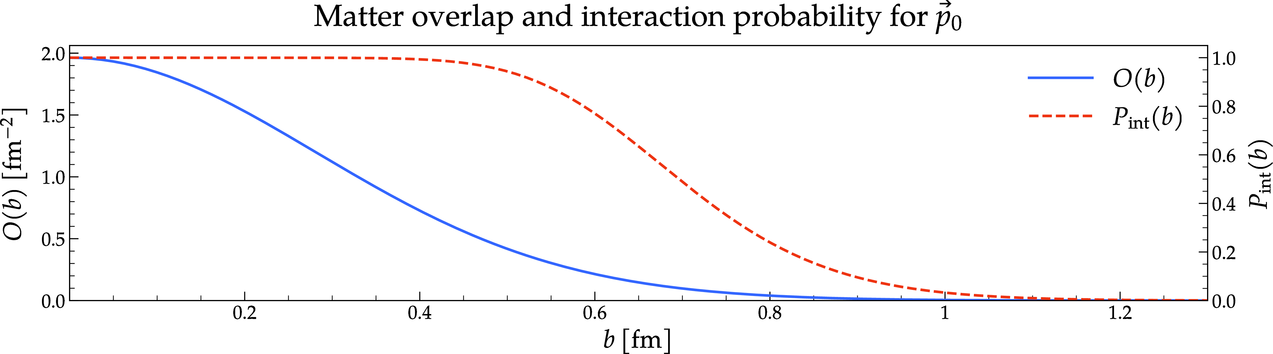
In contrast to the original SZ model, this interpretation affords some physical meaning to the radii of the matter distribution. It is satisfying to note that, after rescaling, the resulting \(R^{\rm eff}_i\) are of the order of 0.1-1 fm.↩︎
Each (non-perturbative) event starts with a signal process, calculated and described through traditional collinear factorisation and perturbative expansion, which also induces a hard scale \(p_\perp^{\rm hard}\). In a first step, the algorithm generates trial pairs of impact parameter \(b\), sampled according to \({\rm d}^2b\,O(b)\), and the scale of the hardest MPI scatter \(p_\perp^{\rm (MPI)}\), obtained from \(\Delta(b)\) with the upper scale the c.m.-energy of the colliding hadrons. If \(p_\perp^{\rm (MPI)}>p_\perp^{\rm hard}\) a new trial pair is generated; conversely, if \(p_\perp^{\rm (MPI)}<p_\perp^{\rm hard}\), the configuration is accepted, the impact parameter is fixed, and the generation of MPIs proceeds with the first additional scatter fixed. In contrast, inclusive (i.e.Minimum Bias) events start by fixing the impact parameter according to \(P_{\rm int}(b)\) and selecting the first scatter freely from \(\Delta(b)\) with a starting scale equivalent to the hadronic c.m.energy. The difference between \(O(b)\) and \(P_{\rm int}(b)\) is shown in Fig. 14; clearly, the overlap \(O(b)\) is described by a significantly sharper distribution than \(P_{\rm int}(b)\), resulting in the underlying event usually driven by smaller impact parameters \(b\) and, correspondingly, a larger partonic activity compared to minimum-bias events. In this publication, however, we have not used minimum-bias data and will instead aim for a combined fit of the model with underlying-event and minimum-bias data in future work.↩︎
Reweighting is supported for both \(\eta_Q\) and \(R\), but expanding the acceptance probability (8 ) to first order in \(\eta_Q^2\Delta\) gives \(\mathcal{P}^{\text{acc}}(\Delta)\approx R\,\eta_Q^2\,\Delta\), so that the two are largely degenerate. We therefore fix \(R=1/9\) and vary \(\eta_Q\) alone.↩︎
The variations of parameters \(R_1\) and \(\alpha_1\) are combined into variations of the matter distribution \(\rho\). For the closure tests, we consider a compact core profile (\(R_1=0.75\,\text{fm}\), \(\alpha_1=0.7\)) and a more diffuse profile (\(R_1=0.95\,\text{fm}\), \(\alpha_1=0.3\)).↩︎
A conventional tune was performed on a grid of dedicated S runs covering the same parameter ranges and observables, serving as an internal cross-check.↩︎