No title
January 01, 1970
Abstract
We formulate a deterministic algorithm for preparing arbitrary multi-qudit states in a definite-weight subspace. By ordering the corresponding computational basis states according to a Gray code for multiset permutations, the state-preparation task is reduced to performing a sequence of controlled 2-qudit Gray rotations. We use this algorithm to prepare exact eigenstates of the \(SU(3)\)-invariant Heisenberg Hamiltonian, whose Bethe ansatz is nested. In particular, we describe the preparation of the Bethe states, which are \(SU(3)\) highest-weight states, as well as their lower-weight descendants. We also consider the preparation of \(SU(d)\) Dicke states and their \(q\)-deformations.
1 Introduction↩︎
The problem of preparing a given multi-qubit quantum state on a quantum computer, using only elementary unitary gates, is an important task in quantum computing [1]. The problem of preparing exact eigenstates (so-called Bethe states) of the spin-1/2 XXZ chain, which are given by the Bethe ansatz [2]–[4], has drawn considerable recent attention [5]–[13]. Since these states are also \(U(1)\)-eigenstates, they have fixed Hamming weight; hence, algorithms for preparing arbitrary states in a fixed Hamming-weight subspace [10], [14]–[17] can in particular be used to prepare such Bethe states. An elegant yet straightforward approach for preparing states in a fixed Hamming-weight subspace, formulated in [14], is to order the corresponding computational basis states according to a so-called Gray code4, which reduces the state-preparation task to performing a sequence of controlled 2-qubit rotations.
Since integrable spin-\(s\) (where \(s \in \{ 1/2, 1, 3/2, \ldots \}\)) generalizations of the XXX model are known [22]–[27], it is natural to consider the problem of preparing the corresponding spin-\(s\) Bethe states. These states are also \(U(1)\)-eigenstates, and therefore have fixed digit sum (rather than fixed Hamming weight, which is limited to the \(s=1/2\) case). An algorithm for preparing arbitrary spin-\(s\) \(U(1)\)-eigenstates (and in particular spin-\(s\) Bethe states) was recently formulated in [28], based on a Gray code for bounded integer compositions [29].
The integrable spin-\(s\) XXX models are based on \(SU(2)\), whose algebra has rank one. Many higher-rank integrable models are also known, see e.g. [30]–[33]. It is therefore also natural to consider the problem of preparing Bethe states for such higher-rank models, where the so-called nesting phenomenon appears [30], [34], [35]. One of our main goals here is to address this problem for the simplest such model, namely, the \(SU(3)\)-invariant Heisenberg chain with periodic boundary conditions. Since these Bethe states are linear combinations of computational basis states with definite weights, we first address the more general problem of preparing arbitrary multi-qudit states in a definite-weight subspace, for which the \(SU(3)\) Bethe states are a special case. Our approach is again based on a Gray code, here for permutations of a multiset [36], which is sketched in Appendix 8.
The remainder of this paper is organized as follows. In Sec. 2 we introduce our notations, define the quantum states of interest and introduce the needed Gray code. We present the state-preparation algorithm in Sec. 3. As simple applications of this result, we consider the preparation of \(SU(d)\) Dicke states [37]–[42] and \(SU_q(d)\) Dicke states [43], [44] in Secs. 4 and 5, respectively. However, these states can be prepared more efficiently by exploiting their symmetry. Our main application, namely the preparation of \(SU(3)\) Bethe states, is presented in Sec. 6; and the preparation of their descendant states is treated in Appendix 9. We are not aware of alternative proposals for preparing such states. We conclude in Sec. 7 with a brief discussion of our results. Implementations in cirq [45] of the state-preparation algorithm and its applications are available on GitHub [46].
2 Basics↩︎
We introduce our notations and define the quantum states of interest in Sec. 2.1. The needed Gray code is introduced in Sec. 2.2.
2.1 The definite-weight subspace↩︎
We consider \(d\)-dimensional qudits, using the computational basis states \(|0\rangle, |1\rangle, \ldots |d-1\rangle\) defined as usual \[|0\rangle=\begin{pmatrix} 1\\ 0\\ 0\\ \vdots\\ 0 \end{pmatrix}\,, \quad| 1\rangle=\begin{pmatrix} 0\\ 1\\ 0\\ \vdots\\ 0 \end{pmatrix} \,, \ldots \,, \quad |d-1\rangle =\begin{pmatrix} 0\\ 0\\ \vdots\\ 0\\ 1 \end{pmatrix} \,. \label{basis}\tag{1}\] We consider \(n\)-qudit states of the form \[|\psi(\vec{k})\rangle = \sum_{w \in \mathfrak{S}_{M(\vec{k})}} a_w | w \rangle \,, \label{states}\tag{2}\] where \(M(\vec{k})\) is the multiset (a set with repeated elements) of \(n\) integers from 0 to \(d-1\) \[M(\vec{k}) =\{ \underbrace{0, \ldots, 0}_{k_{0}}, \underbrace{1, \ldots, 1}_{k_{1}}, \ldots, \underbrace{d-1, \ldots, d-1}_{k_{d-1}}\} = \{ 0^{k_0}, 1^{k_1}, \ldots, (d-1)^{k_{d-1}} \}\,, \label{multiset}\tag{3}\] where \(k_{i}\) is the multiplicity of \(i\) in \(M(\vec{k})\), such that \(M(\vec{k})\) has cardinality \(n\). Hence, \(\vec{k}\) is a \(d\)-dimensional vector such that \[\vec{k} = (k_{0}, k_{1}, \ldots, k_{d-1})\quad \text{with}\quad k_{i} \in \{0, 1, \ldots, n\}\quad \text{and}\quad \sum_{i=0}^{d-1} k_{i} = n\,.\] The sum in 2 is over the set \(\mathfrak{S}_{M(\vec{k})}\) of all unique permutations of \(M(\vec{k})\), whose number \(\mathcal{D}\) is given by the multinomial \[\mathcal{D} = {n \choose \vec{k}} = {n \choose k_{0}, k_{1}, \ldots, k_{d-1}} = \frac{n!}{\prod_{i=0}^{d-1}k_{i}!} \,. \label{dim}\tag{4}\] Moreover, \(w= w_n \ldots w_1\) with \(w_{i} \in \{0, 1, \ldots, d-1\}\) is a permutation in \(\mathfrak{S}_{M(\vec{k})}\) (we will often refer to \(w_1, \ldots, w_n\) as the components of \(w= w_n \ldots w_1\), with corresponding labels \(1, \ldots, n\)), and \(|w\rangle = |w_n\rangle \otimes \ldots \otimes |w_1\rangle\) is the corresponding \(n\)-fold tensor product of computational basis states 1 . Finally, the coefficients \(a_w\) are specified arbitrary complex numbers such that \(|\psi(\vec{k})\rangle\) is normalized \(\sum_{w \in \mathfrak{S}_{M(\vec{k})}} |a_w|^2 = 1\). An example with \(\vec{k}=(2,1,1)\) (and therefore \(d=3, n=4\), and \(M(\vec{k})=\{0, 0, 1, 2\}\)) is \[\begin{align} |\psi(2,1,1)\rangle &= a_{0012}|0012\rangle + a_{0021}|0021\rangle + a_{0120}|0120\rangle + a_{0102}|0102\rangle + a_{0201}|0201\rangle + a_{0210}|0210\rangle \nonumber \\ & + a_{1200}|1200\rangle + a_{1002}|1002\rangle + a_{1020}|1020\rangle + a_{2010}|2010\rangle + a_{2001}|2001\rangle + a_{2100}|2100\rangle \,, \label{d3example} \end{align}\tag{5}\] where tensor products are suppressed as usual.
Let us define the \(U(1)\) generators on a single qudit5 \[\mathbb{k}^{(i)} = |i\rangle\langle i| \,, \qquad i = 0, \ldots, d-1 \,,\] and the corresponding “total” \(U(1)\) generators (acting on all \(n\) qudits) \[\mathbb{K}^{(i)} = \sum_{j=1}^n \mathbb{k}^{(i)}_j \,, \qquad i = 0, \ldots, d-1 \,, \label{U1ops}\tag{6}\] which evidently commute \(\left[ \mathbb{K}^{(i)} \,, \mathbb{K}^{(i')} \right]=0\). The states 2 corresponding to the multiset \(M(\vec{k})\) are simultaneous eigenstates of all the \(\mathbb{K}^{(i)}\) operators, with corresponding eigenvalues \(k_i\) \[\mathbb{K}^{(i)} |\psi(\vec{k}) \rangle = k_i\, |\psi(\vec{k}) \rangle\,, \qquad i = 0, \ldots, d-1 \,;\] these states therefore span the subspace with weight \(\vec{k}\). We will formulate in Sec. 3 an algorithm for preparing such states.
2.2 Gray code for multiset permutations↩︎
In order to prepare the states 2 , we will exploit the remarkable fact (see e.g. [36]) that it is always possible to order the permutations \(w^{[0]}, w^{[1]}, \ldots \in \mathfrak{S}_{M(\vec{k})}\) such that successive permutations \(w^{[l]}\) and \(w^{[l+1]}\) differ by exactly one interchange (swap) of two distinct elements of the multiset \(M(\vec{k})\), that is \[w^{[l+1]} = S_{i^{[l]} j^{[l]}} w^{[l]} \,, \qquad S_{ij} (w_n \ldots w_i \ldots w_j \ldots w_1) = (w_n \ldots w_j \ldots w_i \ldots w_1) \,, \qquad w_i \ne w_j \,, \label{Grayproperty}\tag{7}\] and every unique permutation appears exactly once. To avoid ambiguity, we define \(i, j\) such that \(i > j\). An example for the case \(\vec{k}=(2,1,1)\) corresponding to the state 5 is displayed in Table 1.
| \(l\) | \(w^{[l]}\) | \(i^{[l]}\) | \(j^{[l]}\) | \(w_{i^{[l]}}^{[l]}\) | \(w_{j^{[l]}}^{[l]}\) |
|---|---|---|---|---|---|
| 0 | 0 0 1 2 | 2 | 1 | 1 | 2 |
| 1 | 0 0 2 1 | 3 | 1 | 0 | 1 |
| 2 | 0 1 2 0 | 2 | 1 | 2 | 0 |
| 3 | 0 1 0 2 | 3 | 1 | 1 | 2 |
| 4 | 0 2 0 1 | 2 | 1 | 0 | 1 |
| 5 | 0 2 1 0 | 4 | 2 | 0 | 1 |
| 6 | 1 2 0 0 | 3 | 1 | 2 | 0 |
| 7 | 1 0 0 2 | 2 | 1 | 0 | 2 |
| 8 | 1 0 2 0 | 4 | 2 | 1 | 2 |
| 9 | 2 0 1 0 | 2 | 1 | 1 | 0 |
| 10 | 2 0 0 1 | 3 | 1 | 0 | 1 |
| 11 | 2 1 0 0 |
We will make use here of an algorithm due to Ko and Ruskey [36] for generating permutations of the multiset \(M(\vec{k})\) with the single-swap “Gray” property 7 , which we sketch in Appendix 8. Alternatively, one could search for a Hamiltonian path on the associated graph, see e.g. [21].
3 State-preparation algorithm↩︎
The state 2 can now be re-expressed as \[|\psi(\vec{k})\rangle = \sum_{l=0}^{\mathcal{D}-1} a_l | w^{[l]} \rangle \,, \label{states2}\tag{8}\] where \(w^{[l]} \in \mathfrak{S}_{M(\vec{k})}\) are permutations with the Gray property 7 , and \(a_l := a_{w^{[l]}}\). In order to prepare this state, we first prepare the product state \(|w^{[0]} \rangle\), and then (similarly to [14], [28]) we perform the successive rotations \[|w^{[l]} \rangle \rightarrow \cos(\theta_l) | w^{[l]} \rangle + e^{i \phi_l} \sin(\theta_l) | w^{[l+1]} \rangle \,, \quad l=0, 1, \ldots, \mathcal{D}-2 \,, \label{rotations}\tag{9}\] which results in a state of the form 8 with coefficients \[a_l = \begin{cases} \left(\prod_{j=0}^{l-1} e^{i \phi_j} \sin(\theta_j) \right) \cos(\theta_l) & l = 0, \ldots, \mathcal{D}-2 \\[0.1 in] \prod_{j=0}^{\mathcal{D}-2} e^{i \phi_j} \sin(\theta_j) & l = \mathcal{D}-1 \end{cases} \,. \label{coeffs}\tag{10}\] The equations 10 can be inverted to express the required rotation angles in terms of the specified coefficients \(a_0, \ldots, a_{\mathcal{D}-1}\):6
For the case that all the coefficients are real, all \(\phi_l = 0\), and the angles \(\theta_l\) are given by \[\theta_l = \begin{cases} \mathop{\rm atan2}\nolimits\left( \sqrt{\sum_{j=l+1}^{\mathcal{D}-1} a_j^2}, a_l \right) & l = 0, \ldots, \mathcal{D}-3 \\[0.1 in] \mathop{\rm atan2}\nolimits\left(a_{\mathcal{D}-1}, a_{\mathcal{D}-2} \right) & l = \mathcal{D}-2 \end{cases} \,, \label{thetas-real}\tag{11}\] where \(\mathop{\rm atan2}\nolimits\) is the 2-argument arctangent function, such that \(\mathop{\rm atan2}\nolimits(y,x)={\rm Arg}(x+i y) \in (-\pi, \pi]\).
For the case of complex coefficients, the angles \(\theta_l, \phi_l\) are given by \[\theta_l = \begin{cases} \mathop{\rm atan2}\nolimits\left( \sqrt{\sum_{j=l+1}^{\mathcal{D}-1} |a_j|^2}, |a_l| \right) & l = 0, \ldots, \mathcal{D}-3 \\[0.1 in] \mathop{\rm atan2}\nolimits\left(|a_{\mathcal{D}-1}|, |a_{\mathcal{D}-2}| \right) & l = \mathcal{D}-2 \end{cases} \,, \label{thetas-complex}\tag{12}\] and \[\phi_l = \arg (a_{l+1}) - \arg (a_l)\,, \qquad l = 0, \ldots, \mathcal{D}-2 \,. \label{phis-complex}\tag{13}\]
3.1 Gray gate↩︎
It remains to explain how to implement the \(n\)-qudit rotation 9 . Due to the Gray property 7 , the states \(|w^{[l]}\rangle\) and \(|w^{[l+1]}\rangle\) in 9 are related simply by the interchange of qudits \(i^{[l]}\) and \(j^{[l]}\) in \(|w^{[l]}\rangle\). Hence, the rotation can be accomplished by a transformation, which we call the Gray gate, that performs the corresponding rotation of the relevant pair of qudits.
Specifically, we define the Gray gate \(G_{i,j}^{w_i,w_j}(\theta,\phi)\) such that, when acting on the computational basis states \(|\mu \rangle_i\, |\nu \rangle_j\) with \(\mu, \nu \in \{0, 1, \ldots, d-1\}\) of two qudits labeled by \(i, j \in \{1, 2, \ldots, n\}\) with \(i > j\), it performs the following unitary transformation \[G_{i,j}^{w_i,w_j}(\theta,\phi)\, \left( |\mu \rangle_i\, |\nu \rangle_j \right) = \begin{cases} \cos(\theta)\, |w_i \rangle_i\, |w_j \rangle_j + e^{i \phi} \sin(\theta)\, |w_j \rangle_i\, |w_i \rangle_j & (\mu, \nu) = (w_i, w_j) \\ e^{i \phi} \cos(\theta)\, |w_i \rangle_i\, |w_j \rangle_j - \sin(\theta)\, |w_j \rangle_i\, |w_i \rangle_j & (\mu, \nu) = (w_j, w_i) \\ |\mu \rangle_i\, |\nu \rangle_j & (\mu, \nu) \ne (w_i, w_j)\,, (w_j, w_i) \end{cases} \label{Ggate}\tag{14}\] for given values of \(w_i, w_j \in \{0, 1, \ldots, d-1\}\). From the first line of 14 , we see that this gate performs (when augmented with suitable controls on other qudits, see Sec. 3.1.1) the desired \(n\)-qudit transformation 9 .
The transformation \(G_{i,j}^{w_i,w_j}(\theta,\phi)\) 14 can be implemented with the quantum circuit shown in Fig. 1.

The horizontal wires represent the two \(d\)-level qudits. A circle \(\begin{quantikz}\gateO{\scriptscriptstyle \mu}\end{quantikz}\) denotes a control on the value \(\mu\). The 1-qudit shift gate \({\rm X}\) and its powers are defined as (see e.g. [47]) \[{\rm X}\, |\mu\rangle = |\mu+1 \rangle\,, \qquad {\rm X}^p\, |\mu\rangle = |\mu+p \rangle \,, \label{Xgate}\tag{15}\] where the sums are defined modulo \(d\); these gates are controlled by the upper wire in Fig. 1. Moreover, \(R^{(w_j,w_i)}(\theta,\phi)\) is the 1-qudit unitary gate (Givens rotation) defined by \[\begin{align} R^{(w_j,w_i)}(\theta,\phi) &= \cos(\theta) |w_j\rangle\langle w_j | - \sin(\theta) |w_j\rangle\langle w_i | \nonumber \\ &+ e^{i \phi} \sin(\theta) |w_i\rangle\langle w_j | + e^{i \phi} \cos(\theta) |w_i\rangle\langle w_i | \,, \end{align}\] which in Fig. 1 is controlled by the lower wire. Our Gray gate \(G_{i,j}^{w_i,w_j}(\theta,\phi)\) is a qudit generalization of the qubit RBS gate in [14], and is similar to the Gray gate in [28].
3.1.1 Controls on other qudits↩︎
In order to avoid transforming previously-generated states, it is generally necessary to add to the Gray gates \(G_{i,j}^{w_i,w_j}\) controls on qudits other than \(i, j\). The labels (i.e., addresses, or indices) of these other qudits and the values of the controls can be determined similarly to [14], [28]. Since all the components of \(w^{[l+1]}\) and \(w^{[l]}\) are equal except for those labeled \(i^{[l]}\) and \(j^{[l]}\), the set difference7 \[S^{[l]}:=\{1, \ldots, n\}\backslash \{i^{[l]}, j^{[l]}\}\] is the set of labels of components of \(w^{[l+1]}\) and \(w^{[l]}\) that are equal. Let \(C^{[l]} \subset S^{[l]}\) be the set of labels of components of \(w^{[l+1]}\) and \(w^{[l]}\) that are equal and nonzero; that is \[C^{[l]} := \{ r \in S^{[l]}: w_r^{[l+1]} = w_r^{[l]} \ne 0 \} \,. \label{setC}\tag{16}\] Naively, a control should be placed at all \(r \in C^{[l]}\), with control value \(w_r^{[l+1]} = w_r^{[l]}\).
However, some of these controls are redundant, and can be safely removed. The unnecessary controls can be partially pruned using the following heuristic [28] that generalizes Subroutine 2 in [14]: Let \(U^{[0]}\) be the set of labels of the nonzero “untouched” components of the initial permutation \(w^{[0]}\); that is, \[U^{[0]} := \{ r \in \{1, \ldots, n\} :\;w^{[0]}_r \ne 0 \} \,. \label{setU0}\tag{17}\] At step \(l\), define \(C^{[l]}\) as before 16 ; that is \[C^{[l]} := \{ r \in \{1, \ldots, n\}\backslash \{i^{[l]}, j^{[l]}\}:\;w_r^{[l+1]} = w_r^{[l]} \ne 0 \} \,. \label{setCagain}\tag{18}\] Set \[U^{[l]} = U^{[l-1]}\backslash \{i^{[l]}, j^{[l]}\} \,, \qquad l>0\,,\] and use it to prune \(C^{[l]}\) \[C^{[l]} := C^{[l]}\backslash U^{[l]} \,. \label{setCpruned}\tag{19}\] Again, a control should be placed at all \(r \in C^{[l]}\), with control value \(w_r^{[l+1]} = w_r^{[l]}\). These controls should be added to the (single-controlled) Givens rotation in Fig. 1.
3.2 Summary↩︎
We now summarize our algorithm for preparing the state 2 for a given value of \(\vec{k}\) and for specified coefficients \(a_{w}\).
The permutations \(w^{[0]}, w^{[1]}, \ldots\) of \(M(\vec{k})\) 3 satisfying the Gray property 7 are generated classically, e.g. using the Ko-Ruskey algorithm reviewed in Appendix 8.
The values \((i^{[l]}, j^{[l]})\), \((w_{i^{[l]}}^{[l]}, w_{j^{[l]}}^{[l]})\) and angles \((\theta_l, \phi_l)\) that parametrize the Gray gates 14 , as well as the labels and values of the controls, are computed classically. The values \((i^{[l]}, j^{[l]})\), and therefore \((w_{i^{[l]}}^{[l]}, w_{j^{[l]}}^{[l]})\), follow immediately from 7 . The labels and values of the controls are computed from 17 19 . The angles are given by 11 if all the coefficients \(a_l := a_{w^{[l]}}\) are real, else by 12 and 13 .
The quantum part of the algorithm begins by preparing the state \(|w^{[0]}\rangle\), which is achieved by applying corresponding powers of \({\rm X}\) gates 15 to the all-\(|0\rangle\) state \[|w^{[0]}\rangle = \prod_{r=1}^n {\rm X}^{w^{[0]}_{r}}_r\, |0\rangle^{\otimes n} \,.\]
Finally, the Gray gates 14 , controlled according to 17 19 , are applied successively to prepare the state 2 \[|\psi(\vec{k})\rangle = \overset{\curvearrowleft}{\prod_{l=0}^{\mathcal{D}-2}} G^{[l]} \, |w^{[0]}\rangle \,, \label{genalgorithm}\tag{20}\] where \(G^{[l]} = G_{i^{[l]},j^{[l]}}^{w^{[l]}_{i^{[l]}},w^{[l]}_{j^{[l]}}}(\theta_l,\phi_l)\), and the product goes from right to left with increasing \(l\). Note that no ancillary qudits are needed.
For the example 5 with \(\vec{k} = (2,1,1)\) that is analyzed in Table 1, the quantum circuit 20 is shown in Fig. 2.

The size and depth of the quantum circuit 20 is \(\mathcal{O}(\mathcal{D})\), where \(\mathcal{D}\) is given by 4 . In the worst case \(\vec{k} \sim (\frac{n}{d}\,,\frac{n}{d}\,, \ldots, \frac{n}{d})\), in which case \(\mathcal{D}\) scales exponentially with \(n\): \(\mathcal{D} \sim d^n\). The circuit depth is significantly smaller for typical \(\vec{k}\)-values. For example, for \(\vec{k}\) of the form \[\vec{k} = (n - r x, \overbrace{x, \ldots,x}^r, \overbrace{0, \ldots,0}^{d-r-1}) \,, \qquad 0 < r\le d-1\,, \qquad 0 < x \le \frac{n}{r+1}\,, \label{better}\tag{21}\] (or any permutation thereof) with \(x\) constant (independent of \(n\)), \(\mathcal{D}\) scales polynomially with \(n\): \(\mathcal{D} \sim n^{r x}\).
4 \(SU(d)\) Dicke states↩︎
A simple class of states 2 are so-called \(SU(d)\) Dicke states \(|D^n(\vec{k})\rangle\), defined as uniform superpositions of weight-\(\vec{k}\) computational basis states, with coefficients \[a_w = \frac{1}{\sqrt{\mathcal{D}}} \quad \text{ for all } w \in \mathfrak{S}_{M(\vec{k})} \,, \label{aDicke}\tag{22}\] where \(\mathcal{D}\) is given by 4 . Returning to the example with \(\vec{k}=(2,1,1)\), the corresponding \(SU(3)\) Dicke state is \[\begin{align} |D^4(2,1,1)\rangle &= \frac{1}{\sqrt{12}}\Big(|0012\rangle + |0021\rangle + |0120\rangle + |0102\rangle + |0201\rangle + |0210\rangle \nonumber \\ & + |1200\rangle + |1002\rangle + |1020\rangle + |2010\rangle + |2001\rangle + |2100\rangle \Big)\,. \label{Dickeexample} \end{align}\tag{23}\] Such states have been studied over many years, see e.g. [37]–[42].
The states \(|D^n(\vec{k})\rangle\) are evidently eigenstates of the \(U(1)\) operators 6 \[\mathbb{K}^{(i)} |D^n(\vec{k}) \rangle = k_i\, |D^n(\vec{k}) \rangle\,, \qquad i = 0, \ldots, d-1 \,.\] These states are also ground states of the \(SU(d)\)-invariant Hamiltonian \[H_{SU(d)} = -\sum_{i<j} S_{ij}\,, \qquad S_{ij} = \sum_{a,b=0}^{d-1} e_i^{ab}\, e_j^{ba} \,, \label{DickeHam}\tag{24}\] where \(e^{ab} = |a\rangle \langle b|\) with \(a, b = 0, 1, \ldots, d-1\) is the elementary \(d \times d\) matrix whose only nonzero matrix element is a 1 at position \((a,b)\), and \(e^{ab}_i\) with \(i = 1, 2, \ldots, n\) denotes the corresponding matrix at site \(i\); hence, \(S_{ij}\) is the swap operator for sites \(i\) and \(j\). The Hamiltonian 24 is the quadratic Casimir operator for a chain of \(n\) fundamental representations of \(SU(d)\), up to an additive constant and an overall factor. The states \(|D^n(\vec{k})\rangle\) are eigenstates of this Hamiltonian, with corresponding eigenvalues that are independent of \(d\) and \(\vec{k}\) \[H_{SU(d)}\, |D^n(\vec{k})\rangle = -\tfrac{1}{2}n(n-1)\, |D^n(\vec{k})\rangle \,. \label{DickeEig}\tag{25}\]
We have explicitly verified that, using the coefficients 22 , the circuit 20 indeed prepares the exact states \(|D^n(\vec{k})\rangle\), and we have explicitly verified the property 25 , for various values of \(\vec{k}\), see [46]. The high degree of symmetry of these states can be exploited to prepare these states more efficiently [48]–[51].
5 \(SU_q(d)\) Dicke states↩︎
Another simple class of states 2 are \(SU_q(d)\) Dicke states \(|D^n_q(\vec{k})\rangle\), whose coefficients are given for \(q>0\) by [44] \[a_w = \frac{1}{\sqrt{{n \brack \vec{k}}}} q^{\frac{J(\vec{k})}{2}-\text{inv}(w)} \,, \label{aqDicke}\tag{26}\] where \(\text{inv}(w)\) denotes the inversion number (the minimum number of adjacent transpositions needed to go from the identity permutation to \(w\)) of the permutation \(w\), and \(J(\vec{k})\) is the maximum inversion number. Moreover, \({n \brack \vec{k}}\) denotes the \(q\)-multinomial \[{n \brack \vec{k}}={n \brack k_0,k_1,\dots,k_{d-1}}=\frac{[n]!}{\prod_{i=0}^{d-1}[k_i]!} \,, \label{qmultinomial}\tag{27}\] the \(q\)-factorial is defined for non-negative integers \(n\) by \[[n]!=[n][n-1]\dots[1],\quad\text{with}\quad[0]!=1 \,,\] and \[[x]=\frac{q^x-q^{-x}}{q-q^{-1}}\,, \label{bracket}\tag{28}\] so that \([x]\) is symmetric under \(q\to1/q\). It is clear that \([x]\to x\) as \(q\to1\), so that \([x]\) is a \(q\)-deformation of \(x\). Hence, the states \(|D_q^n(\vec{k})\rangle\) reduce to the \(SU(d)\) Dicke states \(|D^n(\vec{k})\rangle\) in the limit \(q \rightarrow 1\). The case \(d=2\) was first considered in [43]. For the example \(\vec{k}=(2,1,1)\), the corresponding \(SU_q(3)\) Dicke state is \[\begin{align} |D^4_q(2,1,1)\rangle &= \frac{1}{\sqrt{q^5+2q^3+3q+3q^{-1}+2q^{-3}+q^{-5}}} \Big(q^{\frac{5}{2}}|0012\rangle + q^{\frac{3}{2}}|0021\rangle \nonumber \\ & + q^{\frac{1}{2}}|0120\rangle + q^{\frac{3}{2}}|0102\rangle + q^{\frac{1}{2}}|0201\rangle + q^{-\frac{1}{2}}|0210\rangle + q^{-\frac{3}{2}}|1200\rangle \nonumber \\ & + q^{\frac{1}{2}}|1002\rangle + q^{-\frac{1}{2}}|1020\rangle + q^{-\frac{3}{2}}|2010\rangle + q^{-\frac{1}{2}}|2001\rangle + q^{-\frac{5}{2}}|2100\rangle \Big)\,. \label{qDickeexample} \end{align}\tag{29}\] For the case of \(q\) complex, the coefficients are again given by 26 , except that that the normalization factor is computed with \(|q|>0\) [44].
In addition to being eigenstates of the \(U(1)\) operators 6 \[\mathbb{K}^{(i)} |D_q^n(\vec{k}) \rangle = k_i\, |D_q^n(\vec{k}) \rangle\,, \qquad i = 0, \ldots, d-1 \,,\] the states \(|D_q^n(\vec{k})\rangle\) can be shown to be eigenstates of a \(q\)-deformation of the Hamiltonian 24 . Indeed, define \[H_{SU_q(d)} = -\sum_{i=2}^n J_i \,, \qquad J_i = \check{R}_{i-1} + \check{R}_{i-1}\, J_{i-1}\, \check{R}_{i-1} \,, \qquad J_1 = 0\,, \label{qDickeHam}\tag{30}\] where \(J_i\) are \(q\)-deformations of so-called Jucys-Murphy elements (see e.g. [52], [53] and references therein), which have the commutativity property \[\left[ J_i \,, J_j \right] = 0 \,,\] and are expressed in terms of the Hecke operators \[\check{R} = q \sum_a e^{aa} \otimes e^{aa} + \sum_{a\ne b} e^{ab} \otimes e^{ba} + (q-q^{-1})\sum_{a < b} e^{aa} \otimes e^{bb} \,.\] Note that the Hecke operators, which satisfy the relations \[\begin{align} \check{R}_i\, \check{R}_{i+1}\, \check{R}_i &= \check{R}_{i+1}\, \check{R}_i\, \check{R}_{i+1}\,, \nonumber \\ \check{R}_i\, \check{R}_j &= \check{R}_j\, \check{R}_i \,, \qquad |i-j| \ge 2 \,, \nonumber \\ (\check{R}_i - q) (\check{R}_i + q^{-1}) &= 0 \,, \end{align}\] act nontrivially on two sites; \(\check{R}_i\) acts nontrivially on sites \(i\) and \(i+1\). The Hamiltonian 30 has only \(U(1)^{d-1}\) (rather than \(SU(d)\)) symmetry. In the limit \(q \rightarrow 1\), the Hamiltonian 30 reduces to 24 . The states \(|D_q^n(\vec{k})\rangle\) are eigenstates of the Hamiltonian 30 \[H_{SU_q(d)}\, |D_q^n(\vec{k})\rangle = E\, |D_q^n(\vec{k})\rangle \,, \qquad E = -\sum_{i=0}^{n-2} (i+1) q^{2n-3-2i} \,, \label{qDickeEig}\tag{31}\] which does not seem to have been previously noticed in the physics literature.
We have explicitly verified that, using the coefficients 26 , the circuit 20 indeed prepares the exact states \(|D_q^n(\vec{k})\rangle\), and we have explicitly verified the property 31 , for various values of \(\vec{k}\) and \(q\), see [46]. The high degree of symmetry of these states can be exploited to prepare these states more efficiently [44].
6 \(SU(3)\) Bethe states↩︎
The \(SU(2)\)-invariant Heisenberg Hamiltonian with periodic boundary conditions, whose integrability was revealed by Bethe [2], has a natural generalization to \(SU(d)\) \[H= \sum_{i=1}^n \left(S_{i,i+1} - \mathbb{I}\right) \,, \qquad S_{n,n+1} = S_{n,1} \,, \label{HeisHam}\tag{32}\] where \(S_{ij}\) is the swap operator for \(d\)-level qudits defined in 24 . Remarkably, this \(SU(d)\)-invariant Hamiltonian is integrable for all integer values \(d \ge 2\) [34], [35]. However, for \(d>2\), the Bethe ansatz solution entails an intricate nesting procedure. For simplicity, we focus here on the case \(d=3\), where the nesting phenomenon first appears.
An expression for the \(SU(3)\) Bethe states (exact eigenstates of the Hamiltonian 32 with \(d=3\) in terms of two sets of Bethe roots \(\{u_1, \ldots, u_{m_1} \}\) and \(\{v_1, \ldots, v_{m_2}\}\) with \(0\le m_2 \le m_1 \le n\), known as coordinate Bethe ansatz) is given by [30], [34], [35], [54] \[|\{u_1, \ldots, u_{m_1} \}; \{v_1, \ldots, v_{m_2} \} \rangle = \sum_{1 \le x_1 < \ldots < x_{m_1} \le n}\; \sideset{}{'}\sum_{\alpha_1, \ldots, \alpha_{m_1} = 1}^{2} f\overset{(\alpha_1, \ldots, \alpha_{m_1})}{(x_1, \ldots, x_{m_1}}; \{ u\}, \{v\})\, e_{x_1}^{\alpha_1,0} \cdots e_{x_{m_1}}^{\alpha_{m_1},0} |0\rangle^{\otimes n} \,, \label{BA1}\tag{33}\] where the prime on the summation over \(\alpha\)’s denotes the restriction \[\sum_{j=1}^{m_1} \delta_{2, \alpha_j} = m_2 \,;\] that is, the summation is over all \(\alpha_j \in \{1, 2\}\) such that the number of \(\alpha\)’s with value 2 is \(m_2\), and the \(m_1-m_2\) remaining \(\alpha\)’s have value 1. Moreover, the matrices \(e^{ab}_i\) in 33 are the same as in 24 ; hence, \(e^{10} |0\rangle = |1\rangle\) and \(e^{20} |0\rangle = |2\rangle\). We define \(y_1, \ldots, y_{m_2}\) with \(y_l \in \{1, \ldots, m_1\}\) as the positions of those \(\alpha\)’s with value 2; that is, \[\alpha_{y_l}=2 \,, \qquad l = 1, \ldots, m_2 \,. \label{ydef}\tag{34}\] The function \(f\) in 33 is given by \[\begin{align} f\overset{(\alpha_1, \ldots, \alpha_{m_1})}{(x_1, \ldots, x_{m_1}}; \{ u\}, \{v\}) &= \sum_{P \in \mathfrak{S}_{m_1}} \sum_{Q \in \mathfrak{S}_{m_2}} \Big\{ \varepsilon(P) \varepsilon(Q) A(u_{P(1)}, \ldots, u_{P(m_1)})\, B(v_{Q(1)}, \ldots, v_{Q(m_2)}) \nonumber \\ & \times \prod_{j=1}^{m_1} \left(\frac{u_{P(j)}+\frac{i}{2}}{u_{P(j)}-\frac{i}{2}}\right)^{x_j} \prod_{l=1}^{m_2} \Phi(v_{Q(l)}; u_{P(1)}, \ldots, u_{P(y_l)}) \Big\} \,, \label{BA2} \end{align}\tag{35}\] where the sums are over the sets \(\mathfrak{S}_{m_1}\) and \(\mathfrak{S}_{m_2}\) of all permutations of \(\{1, \ldots, m_1\}\) and \(\{1, \ldots, m_2\}\), respectively; and \(\varepsilon=\pm 1\) denotes the sign of a permutation. The functions \(A, B, \Phi\) in 35 are given by \[\begin{align} A(u_1, \ldots, u_{m_1}) &= \prod_{1 \le a < b \le m_1} (u_a - u_b +i) \,, \nonumber\\ B(v_1, \ldots, v_{m_2}) &= \prod_{1 \le a < b \le m_2} (v_a - v_b +i) \,, \nonumber\\ \Phi(v; u_1, \ldots, u_y) &= \frac{1}{v-u_y-\frac{i}{2}} \prod_{l=1}^{y-1}\frac{v-u_l+\frac{i}{2}}{v-u_l-\frac{i}{2}} \,. \label{BA3} \end{align}\tag{36}\] The Bethe roots \(\{u_1, \ldots, u_{m_1} \}\) and \(\{v_1, \ldots, v_{m_2}\}\) are solutions of the Bethe equations \[\begin{align} \left(\frac{{u_j}-\frac{i}{2}}{{u_j}+\frac{i}{2}}\right)^n &= \prod_{l \ne j}^{m_1} \frac{u_j - u_l -i}{u_j - u_l +i} \prod_{l =1}^{m_2} \frac{u_j - v_l +\frac{i}{2}}{u_j - v_l -\frac{i}{2}} \,, \qquad j = 1, \ldots, m_1 \,, \tag{37} \\ 1 &= \prod_{l=1}^{m_1} \frac{v_j - u_l + \frac{i}{2}}{v_j - u_l - \frac{i}{2}} \prod_{l\ne j}^{m_2} \frac{v_j - v_l -i }{v_j - v_l +i} \,, \qquad j = 1, \ldots, m_2 \,. \tag{38} \end{align}\] Various approaches have been developed for solving such equations. For small values of \(n\), a particularly useful approach is to exploit the corresponding Q-system [55].
The Bethe states 33 are exact eigenstates of the \(d=3\) Hamiltonian 32 \[H\, |\{u \}; \{v \} \rangle = E\, |\{u \}; \{v \} \rangle \,,\] with corresponding energy \[E = -\sum_{j=1}^{m_1} \frac{1}{u_j^2 + \frac{1}{4}} \,, \label{energyBA}\tag{39}\] as well as of the \(U(1)\) operators 6 \[\mathbb{K}^{(i)} |\{u \}; \{v \} \rangle = k_i\, |\{u \}; \{v \} \rangle\,, \qquad i = 0, 1, 2 \,,\] where \[k_0 = n - m_1 \,, \qquad k_1 = m_1 - m_2 \,, \qquad k_2 = m_2 \,. \label{kBA}\tag{40}\]
The Bethe state 33 can be cast in the form 2 , with \(\vec{k}\) given by 40 , and with coefficients \(a_w\) given (up to an overall normalization factor) by \[a_{w_n \ldots w_1} = f\overset{(\alpha_1, \ldots, \alpha_{m_1})}{(x_1, \ldots, x_{m_1}}; \{ u\}, \{v\}) \,, \label{awBA}\tag{41}\] where the \(x_i\)’s are the positions of the nonzero \(w_i\)’s, and the \(\alpha\)’s are the values of those nonzero \(w_i\)’s.
Using Bethe roots8 obtained using the \(SU(3)\) Q-system [55], we have explicitly verified that the circuit 20 indeed prepares exact eigenstates of the Hamiltonian 32 , with corresponding eigenvalue 39 , for various values of \(n, m_1, m_2\), see [46].
The Bethe states 33 are \(SU(3)\) highest-weight states. The lower-weight descendant states can be prepared similarly to the Bethe states, except with different amplitudes, as shown in Appendix 9.
7 Discussion↩︎
We have formulated an algorithm for deterministically preparing arbitrary multi-qudit states in a weight-\(\vec{k}\) subspace 2 . This algorithm is similar to those for preparing multi-qubit states in a fixed Hamming-weight subspace [14] and spin-\(s\) \(U(1)\) eigenstates [28], in the sense that all three algorithms exploit Gray codes to reduces the state-preparation task to performing a sequence of controlled 2-qudit Gray rotations. However, these algorithms all requires different Gray codes, and therefore they differ in crucial details. We cannot help but marvel at the fact that the needed Gray codes [18], [29], [36] were discovered decades earlier in the mathematics/computer science communities.
We have demonstrated that this algorithm can in principle be used to prepare nested Bethe states, which therefore opens the way for preparing Bethe states for many classes of integrable models. Indeed, in our implementation of the algorithm using the cirq statevector simulator [45], one simply inputs the system size and Bethe roots, and the output is the corresponding explicit Bethe statevector [46]. However, as emphasized in [10], [28], this coordinate-Bethe-ansatz approach has a high classical overhead for computing the coefficients \(a_w\), and therefore for computing the corresponding angles of the Gray rotations. Moreover, the quantum complexity of the algorithm is also high. Hence, this approach is not practical for large system size.
We note that relatively few explicit expressions for nested coordinate Bethe ansatz wavefunctions are available in the literature, presumably partly because of their unwieldiness, as well as due to the advent of nested algebraic Bethe ansatz [56]. Indeed, we did not succeed to find anywhere in the literature the explicit expression 35 36 for the \(SU(3)\) wavefunction, which we had to reconstruct from [30], [34], [35], [54]. Hence, we expect that new nested coordinate Bethe ansatz results may be needed in order to prepare in this way eigenstates of other integrable models, such as those with anisotropy, boundaries, or yet-higher rank.
It remains to be seen whether an alternative Bethe-state-preparation approach based instead on algebraic Bethe ansatz [4], [8], [9], [11], [56] can yield similarly explicit results while overcoming the challenges of high classical and quantum complexity.
Acknowledgements↩︎
We thank Eric Ragoucy for valuable correspondence, and for sharing with us the unpublished manuscript [57]. RN is supported in part by the National Science Foundation under grant PHY 2310594, and by a Cooper fellowship.
8 A Ko-Ruskey Gray code for multiset permutations↩︎
It is convenient to represent the permutations of a multiset \(M(\vec{k})\) by an upside-down tree, as shown in Fig. 3 for \(\vec{k}=(2,1,1)\), such that
every path from the root down to a leaf spells out one of the permutations. In the naive recursive scheme shown in this figure (corresponding to the GenBag algorithm in [36]), the children (the remaining available elements of the multiset) at each node are selected in strictly increasing order, resulting in a standard lexicographic (dictionary) ordering of the permutations (reading the bold
permutations across the bottom from left to right), which does not satisfy the single-swap (Gray) property 7 .
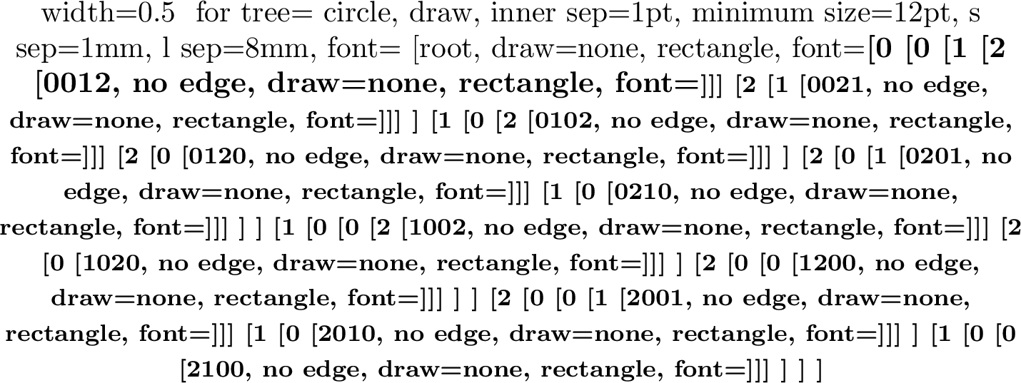
An ingenious way to ensure the single-swap property between successive permutations is to assign signs \((\pm)\) to the nodes: the children at a plus-node \((+)\) are selected in
increasing order, while the children at a negative-node \((-)\) are selected in decreasing order. (For a node with only one child, the sign is irrelevant.) In the simplest scheme (GenAltA in [36]), illustrated in Fig. 4 for \(\vec{k}=(2,1,1)\), the nodes are assigned signs that
alternate across each level, starting with \(+\) on the left. For example, at level 1 (just below the root), the signs from left to right are \(+, -, +\). The resulting permutations
(reading the bold permutations across the bottom from left to right) indeed have the single-swap (Gray) property 7 . Optimized versions of this algorithm are also presented in [36].
![Figure 4: Tree for multiset permutations with the Gray property for \vec{k}=(2,1,1). Note that the signs of the nodes alternate across each level. (Adapted from Fig. 3 in [36].)](/article/2606.24659/_pdflatex/arfmwexb.png "fig:")
9 Descendant states↩︎
The on-shell Bethe states 33 are \(SU(3)\) highest-weight states that are annihilated by the raising operators \[E^{01}\, |\{u \}; \{v \} \rangle = 0 \,, \qquad E^{02}\, |\{u \}; \{v \} \rangle = 0 \,, \qquad E^{12}\, |\{u \}; \{v \} \rangle = 0 \,, \label{su3hw}\tag{42}\] where \[E^{ab} = \sum_{i=1}^{n} e^{ab}_i \,, \qquad e^{ab} = |a\rangle \langle b| \,.\] Together with their lower-weight descendants, obtained by acting on the highest-weight states with lowering operators \(E^{10}, E^{20}, E^{21}\), they form \(SU(3)\) irreducible representations with the common energy 39 .
We consider here the problem of preparing such descendant states on a quantum computer. Directly applying lowering operators on Bethe states is not an option, since the lowering operators are not unitary. Moreover, introducing additional infinite Bethe roots is also not an option, since the corresponding amplitudes 35 then become indeterminate. As a warm-up, we first treat the simpler \(SU(2)\) case in Sec. 9.1 before moving on to the \(SU(3)\) case in Sec. 9.2. We shall see that the descendant states can be prepared similarly to the Bethe states, except with different amplitudes, see 50 51 .
9.1 \(SU(2)\) descendants↩︎
For the \(SU(2)\)-invariant spin-1/2 Heisenberg Hamiltonian of length \(n\) with periodic boundary conditions, let us write an (unnormalized) on-shell Bethe state with \(m\) Bethe roots as \[|B_m\rangle = \sum_{\substack{Y \subset \{1, \ldots, n\}\\ |Y|=m}} f(Y) |Y\rangle \,, \label{su2BetheState}\tag{43}\] where the sum is over all subsets \(Y\) of \(\{1, \ldots, n\}\) with cardinality \(|Y|= m \in [0, \frac{n}{2}]\); \(|Y\rangle\) is the \(n\)-qubit computational basis state with 1’s at positions \(Y\) and 0’s elsewhere; and \(f(Y)\) is the coordinate Bethe ansatz wavefunction, which depends on the \(m\) Bethe roots. These states are \(SU(2)\) highest-weight states [4] \[S^+\, |B_m\rangle = 0 \,, \qquad S^+ = E^{01} \,,\] with \(s=s^z =\frac{n}{2}-m\), where \(s\) is the spin and \(s^z\) is the eigenvalue of \(S^z = \sum_{i=1}^n \frac{1}{2}\sigma_i^z\).
The \(SU(2)\) descendant states are obtained by repeatedly applying the lowering operator \(S^- = E^{10}\) to the Bethe state. Observe that9 \[\left(S^- \right)^\ell \, |Y\rangle \propto \sum_{\substack{Z \subset \{1, \ldots, n\}\\ |Z|=\ell\,, \;Z \cap Y = \emptyset}} |Y \cup Z \rangle = \sum_{\substack{X \subset \{1, \ldots, n\}\\ |X|=\bar{m}\,, \;X \supset Y}} |X \rangle \,, \label{observe}\tag{44}\] where \(X:=Y \cup Z\) is the set of positions of 1’s, whose cardinality is \(\bar{m} := m + \ell\). Applying \(\left(S^- \right)^\ell\) to the Bethe state 43 , we obtain \[\begin{align} \left(S^- \right)^\ell \, |B_m\rangle &= \sum_{\substack{Y \subset \{1, \ldots, n\}\\ |Y|=m}} f(Y)\, \left(S^- \right)^\ell |Y\rangle \,, \nonumber \\ &\propto \sum_{\substack{Y \subset \{1, \ldots, n\}\\ |Y|=m}} f(Y)\, \sum_{\substack{X \subset \{1, \ldots, n\}\\ |X|=\bar{m}\,, \;X \supset Y}} |X \rangle \,, \nonumber \\ &= \sum_{\substack{X \subset \{1, \ldots, n\}\\ |X|=\bar{m}}} \left( \sum_{\substack{Y \subset X\\ |Y|=m}} f(Y) \right) |X\rangle \,, \end{align}\] where the result 44 has been used in the second line, and the order of summations has been interchanged in the last line. We conclude that the \(SU(2)\) descendant states are given by \[\left(S^- \right)^\ell \, |B_m\rangle \propto \sum_{\substack{X \subset \{1, \ldots, n\}\\ |X|= \bar{m}}} F(X) |X\rangle \,, \qquad F(X) = \sum_{\substack{Y \subset X\\ |Y|=m}} f(Y) \,, \label{su2Descedants}\tag{45}\] which can be prepared on a quantum computer similarly to the Bethe state 43 itself [10], [14].
As a simple example of the result 45 , let us consider the case \(m=0\), for which the Bethe state is the reference state \(|B_0\rangle = |0\rangle^{\otimes n}\), with \(Y=\emptyset\) and \(f(Y)=1\). It follows from 45 that \(F(X)=1\), hence \[\left(S^- \right)^\ell \, |0\rangle^{\otimes n} \propto \sum_{\substack{X \subset \{1, \ldots, n\}\\ |X|= \ell}} |X\rangle \,,\] which we recognize as ordinary \(SU(2)\) Dicke states with Hamming weight \(\ell\).
9.2 \(SU(3)\) descendants↩︎
Let us now rewrite the unnormalized Bethe states 33 , analogously to 43 , as \[|B_{m_1, m_2}\rangle = \sum_{\substack{Y \subset \{1, \ldots, n\}\\ |Y|=m_1}} \sum_{\substack{Y_2 \subset Y\\ |Y_2|=m_2}} f(Y_2 \subset Y)\, |Y_2 \subset Y\rangle \,, \label{su3BetheState}\tag{46}\] where \(|Y_2 \subset Y\rangle\) denotes the \(n\)-qutrit computational basis state with 2’s at positions \(Y_2\), 1’s at positions \(Y\backslash Y_2\), and 0’s elsewhere; and \(f(Y_2 \subset Y)\) corresponds to the amplitude 35 . For these basis states, the number of 2’s is \(m_2\), and the number of 1’s is \(m_1-m_2\). As already noted, \(|B_{m_1, m_2}\rangle\) is an \(SU(3)\) highest-weight state 42 .
The \(SU(3)\) descendant states of the Bethe state 46 can be obtained in terms of the Poincaré-Birkhoff-Witt (PBW) basis [58] as \[\left( E^{21} \right)^a\, \left( E^{20} \right)^b\, \left( E^{10} \right)^c\, |B_{m_1, m_2}\rangle \,. \label{PBW}\tag{47}\] Compared with \(|B_{m_1, m_2}\rangle\), these states have \(\ell_2\) additional 2’s, and \(\ell_1 - \ell_2\) additional 1’s, where \[\ell_1 := b + c\,, \qquad \ell_2 := a + b \,. \label{ell1ell2}\tag{48}\] Hence, for the descendant state 47 , the total number of 2’s is \(\bar{m}_2 := m_2 + \ell_2 = m_2 + a + b\); and the total number of 1’s is \(\bar{m}_1-\bar{m}_2\), where \(\bar{m}_1 := m_1 + \ell_1 = m_1 + b + c\).
Let us apply the lowering operators in 47 on \(|Y_2 \subset Y\rangle\) step-by-step: \[\left( E^{10} \right)^c\, |Y_2 \subset Y\rangle \propto \sum_{\substack{Z_1 \subset \{1, \ldots, n\}\backslash Y\\ |Z_1|=c\,, \;Z_1 \cap Y = \emptyset}} |Y_2 \subset (Y \cup Z_1) \rangle \,,\]
\[\begin{align} \left( E^{20} \right)^b\, \left( E^{10} \right)^c\, |Y_2 \subset Y\rangle &\propto \sum_{\substack{Z_1 \subset \{1, \ldots, n\}\backslash Y\\ |Z_1|=c\,, \;Z_1 \cap Y = \emptyset}} \left( E^{20} \right)^b\, |Y_2 \subset (Y \cup Z_1) \rangle \nonumber \\ &\propto \sum_{\substack{Z_1 \subset \{1, \ldots, n\}\backslash Y\\ |Z_1|=c\,, \;Z_1 \cap Y = \emptyset}} \quad \sum_{\substack{Z \subset \{1, \ldots, n\}\backslash (Y\cup Z_1)\\ |Z|=b\,, \;Z \cap (Y \cup Z_1) = \emptyset}} |(Y_2 \cup Z) \subset (Y \cup Z_1 \cup Z) \rangle \,, \end{align}\]
\[\begin{align} &\left( E^{21} \right)^a\, \left( E^{20} \right)^b\, \left( E^{10} \right)^c\, |Y_2 \subset Y\rangle \nonumber \\ &\propto \sum_{\substack{Z_1 \subset \{1, \ldots, n\}\backslash Y\\ |Z_1|=c\,, \;Z_1 \cap Y = \emptyset}} \quad \sum_{\substack{Z \subset \{1, \ldots, n\}\backslash (Y\cup Z_1)\\ |Z|=b\,, \;Z \cap (Y \cup Z_1) = \emptyset}} \left( E^{21} \right)^a\, |(Y_2 \cup Z) \subset (Y \cup Z_1 \cup Z) \rangle \nonumber \\ &\propto \sum_{\substack{Z_1 \subset \{1, \ldots, n\}\backslash Y\\ |Z_1|=c\,, \;Z_1 \cap Y = \emptyset}} \quad \sum_{\substack{Z \subset \{1, \ldots, n\}\backslash (Y\cup Z_1)\\ |Z|=b\,, \;Z \cap (Y \cup Z_1) = \emptyset}} \quad \sum_{\substack{Z_2 \subset ((Y\backslash Y_2) \cup Z_1 ) \\ |Z_2|=a}} |(Y_2 \cup Z \cup Z_2) \subset (Y \cup Z_1 \cup Z) \rangle \nonumber \\ &= \sum_{\substack{Z_1 \subset \{1, \ldots, n\}\backslash Y\\ |Z_1|=c\,, \;Z_1 \cap Y = \emptyset}} \quad \sum_{\substack{Z \subset \{1, \ldots, n\}\backslash (Y\cup Z_1)\\ |Z|=b\,, \;Z \cap (Y \cup Z_1) = \emptyset}} \quad \sum_{\substack{Z_2 \subset ((Y\backslash Y_2) \cup Z_1 ) \\ |Z_2|=a}} |X_2 \subset X \rangle \,, \label{observe2} \end{align}\tag{49}\] where \(X_2:=Y_2 \cup Z \cup Z_2\) and \(X:=Y \cup Z_1 \cup Z\), whose cardinalities are \(\bar{m}_2\) and \(\bar{m}_1\) (defined below 48 ), respectively. Note that \(X_2\) is the set of positions of 2’s, and \(X\backslash X_2\) is the set of positions of 1’s. It is helpful to visualize the various subsets in a Venn-type diagram as in Fig. 5.
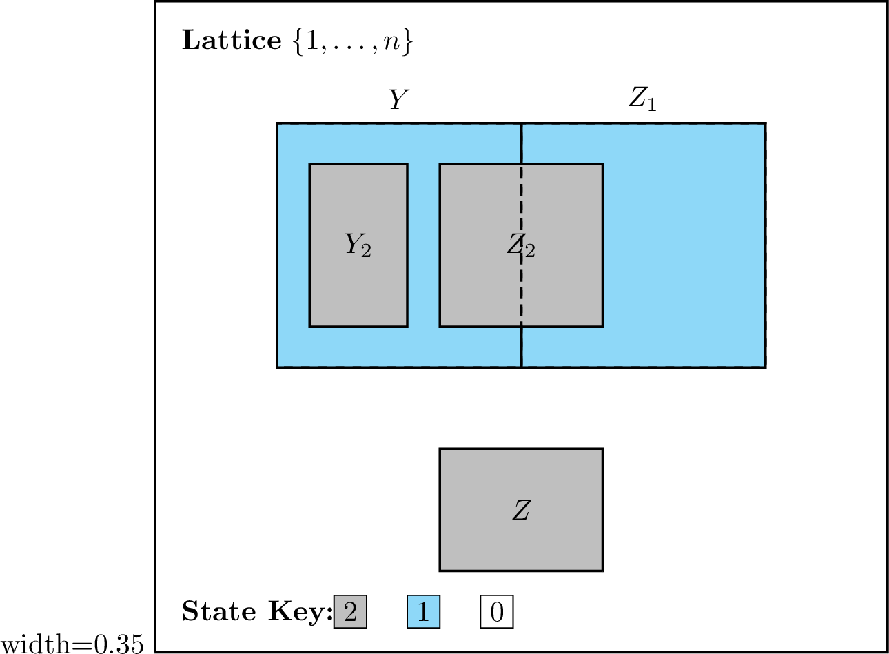
Recalling 46 , we obtain \[\begin{align} &\left( E^{21} \right)^a\, \left( E^{20} \right)^b\, \left( E^{10} \right)^c\, |B_{m_1, m_2}\rangle \nonumber \\ &= \sum_{\substack{Y \subset \{1, \ldots, n\}\\ |Y|=m_1}} \sum_{\substack{Y_2 \subset Y\\ |Y_2|=m_2}} f(Y_2 \subset Y)\, \left( E^{21} \right)^a\, \left( E^{20} \right)^b\, \left( E^{10} \right)^c\, |Y_2 \subset Y\rangle \nonumber \\ &\propto \sum_{\substack{Y \subset \{1, \ldots, n\}\\ |Y|=m_1}} \sum_{\substack{Y_2 \subset Y\\ |Y_2|=m_2}} f(Y_2 \subset Y)\, \sum_{\substack{Z_1 \subset \{1, \ldots, n\}\backslash Y\\ |Z_1|=c\,, \;Z_1 \cap Y = \emptyset}} \quad \sum_{\substack{Z \subset \{1, \ldots, n\}\backslash (Y\cup Z_1)\\ |Z|=b\,, \;Z \cap (Y \cup Z_1) = \emptyset}} \quad \sum_{\substack{Z_2 \subset ((Y\backslash Y_2) \cup Z_1 ) \\ |Z_2|=a}} |X_2 \subset X \rangle \nonumber \\ &= \sum_{\substack{X \subset \{1, \ldots, n\}\\ |X|=\bar{m}_1}} \sum_{\substack{X_2 \subset X\\ |X_2|=\bar{m}_2}} \left( \sum_{\substack{Z \subset X_2 \\ |Z|=b}} \sum_{\substack{Y_2 \subset (X_2\backslash Z) \\ |Y_2|=m_2}} \sum_{\substack{Y \subset (X\backslash Z) \\ |Y|=m_1\,, \;Y \supset Y_2}} f(Y_2 \subset Y) \right) |X_2 \subset X \rangle \,, \end{align}\] where the result 49 has been used in the second step, and the order and structure of summations have been changed in the last step. (For given sets \(X\) and \(X_2 \subset X\), we first fix \(Z \subset X_2\), which has no elements in common with any of the sets \(Y, Y_2, Z_1, Z_2\). The fact \(X_2\backslash Z = Y_2 \cup Z_2\) implies that \(Y_2 \subset (X_2\backslash Z)\); and the fact \(X\backslash Z = Y \cup Z_1\) implies that \(Y \subset (X\backslash Z)\). Once \(Y_2\) and \(Y\) are fixed, then \(Z_1\) and \(Z_2\) are also fixed, since \(Z_1 = X\backslash (Z \cup Y)\) and \(Z_2 = X_2\backslash (Z \cup Y_2)\), see Fig. 5.) We conclude that the \(SU(3)\) descendant states are given by \[\left( E^{21} \right)^a\, \left( E^{20} \right)^b\, \left( E^{10} \right)^c\, |B_{m_1, m_2}\rangle \propto \sum_{\substack{X \subset \{1, \ldots, n\}\\ |X|=\bar{m}_1}} \sum_{\substack{X_2 \subset X\\ |X_2|=\bar{m}_2}} F(X_2 \subset X)\, |X_2 \subset X \rangle \,, \label{su3Descendants}\tag{50}\] where \[F(X_2 \subset X) = \sum_{\substack{Z \subset X_2 \\ |Z|=b}} \sum_{\substack{Y_2 \subset (X_2\backslash Z) \\ |Y_2|=m_2}} \sum_{\substack{Y \subset (X\backslash Z) \\ |Y|=m_1\,, \;Y \supset Y_2}} f(Y_2 \subset Y) \,. \label{su3DescendantsF}\tag{51}\] The states 50 can be prepared on a quantum computer similarly to the Bethe state 46 itself, except now with the amplitudes \(F(X_2 \subset X)\) 51 that (like the amplitudes \(f(Y_2 \subset Y)\) of the Bethe state) are to be computed classically. In principle, all eigenstates of the Hamiltonian 32 corresponding to regular (non-singular) solutions of the Bethe equations 37 38 can be prepared in this way.
As a simple example of the result 50 , let us consider the case \(m_1=m_2=0\), for which the Bethe state is the reference state \(|B_{0,0}\rangle = |0\rangle^{\otimes n}\), with \(Y_2=Y=\emptyset\) and \(f(Y_2 \subset Y)=1\). All of the descendant states of \(|B_{0,0}\rangle\) can be obtained with \(b=0\), for which case 51 implies that \(F(X_2 \subset X)=1\), and we obtain \[\left( E^{21} \right)^a\, \left( E^{10} \right)^c\, |0\rangle^{\otimes n} \propto \sum_{\substack{X \subset \{1, \ldots, n\}\\ |X|= c}} \sum_{\substack{X_2 \subset X\\ |X_2|=a}} |X_2 \subset X \rangle \,,\] which we recognize as \(SU(3)\) Dicke states (see Sec. 4) with weight \(\vec{k}=(n-c,c-a,a)\).
References↩︎
mxz866@miami.edu↩︎nepomechie@miami.edu↩︎Corresponding author↩︎
A Gray code due to Ehrlich [18] is used in [14]. For reviews of Gray codes, see e.g. [19]–[21].↩︎
Only \(d-1\) of these generators are independent, since \(\sum_{i=0}^{d-1}\mathbb{k}^{(i)} = \mathbb{I}\).↩︎
All the coefficients should be rescaled \(a_l \mapsto a_l\, |a_0|/a_0\), so that \(a_0\) is real.↩︎
By definition, the set difference \(A\backslash B\) is the set of elements in set \(A\) that are not in set \(B\).↩︎
For simplicity, we restrict to regular (non-singular) Bethe roots.↩︎
Here and below we do not pay attention to overall factors, as indicated with the proportionality symbol \(\propto\).↩︎