Electrical-Circuit Simulation of the Uhlmann Phase
June 23, 2026
Abstract
The Uhlmann phase extends the concept of geometric phases to mixed quantum states through a parallel-transport condition on purification amplitudes, but its experimental realization has so far required sophisticated quantum platforms with carefully engineered auxiliary degrees of freedom. In this work, we reformulate the Uhlmann parallel-transport condition as a linear matrix differential equation and vectorize it to obtain an effective dynamical generator. This generator can be directly mapped onto the admittance matrix of a classical RC circuit, thereby translating the Uhlmann dynamics into the evolution of circuit node voltages. We illustrate the mapping using the equatorial-loop model and, via a rotating-frame transformation followed by a real decomposition, derive a time-independent, real-valued dynamical system suitable for analog implementation. LTspice simulations of the resulting active RC network faithfully reproduce the Uhlmann geometric phase and its topological transition at the critical purity, demonstrating that classical electrical circuits offer a simple and accessible platform for probing mixed-state geometric phases.
1 Introduction↩︎
Geometric phases are fundamental to the topological characterization of quantum systems [1], [2]. The Berry phase, acquired during adiabatic cyclic evolution of pure states, underpins the modern classification of topological insulators and superconductors through the Berry curvature and related invariants [3]–[17]. These phases have been observed in a variety of platforms, including superconducting qubits, ultracold atoms, and photonic systems [18]–[20]. Nevertheless, the Berry-phase framework is inherently restricted to pure states and cannot directly describe mixed states arising from environmental coupling or thermal fluctuations.
For mixed states, a mathematically rigorous generalization is provided by the Uhlmann phase [21], [22], which is constructed based on the purification \(W\) (the counterpart of pure-state wavefunctions) of density matrices via \(\rho=WW^\dagger\) (similar to \(\rho=|\psi\rangle\langle\psi|\) for pure states) and a parallel-transport condition imposed on \(W\). This framework has become central to the study of topological phenomena at finite temperature and in open quantum systems [23]–[29]. An interferometric formulation of mixed-state geometric phases was also developed by Sjöqvist et al. and demonstrated in NMR experiments [30], [31]. Both approaches extend geometric phases beyond pure states, yet they rest on different physical principles. Here we adopt the Uhlmann framework. While the Berry phase can be understood via parallel transport of pure states, the Uhlmann parallel-transport condition acts in the enlarged purification space and is not automatically satisfied under standard Hamiltonian dynamics [32], [33], thus requiring auxiliary purification degrees of freedom and engineered evolution protocols. The Uhlmann phase has been observed in advanced quantum platforms such as superconducting circuits, photonic quantum walks, and programmable quantum processors [34]–[37]. However, in those experiments the Uhlmann phase was extracted either from the purified state, an entangled state in the system-ancilla space, or directly from interferometric or tomographic measurements on the density matrix, without implementing the parallel transport of the purification itself. This leaves open the possibility of a simulator that faithfully implements the Uhlmann parallel-transport dynamics at the level of the purification, which is the gap addressed by the classical electrical-circuit platform proposed in this work.
A central obstacle to the direct physical realization of Uhlmann parallel transport is that the purification \(W\) of a density matrix is generally a non-Hermitian matrix, whose dynamical implementation does not follow from standard Hamiltonian evolution. In this work, we circumvent this difficulty by reformulating the Uhlmann parallel-transport condition as a linear evolution equation for \(W\), and then applying a vectorization procedure that converts this matrix equation into an ordinary linear dynamical system. The resulting vectorized equation is structurally identical to the Kirchhoff-law description of classical RC circuits, thus opening the possibility of simulating Uhlmann process with electrical networks. This approach is motivated by the broader development of electrical-circuit platforms as a versatile tool for emulating topological and quantum-inspired phenomena, through the mapping between effective Hamiltonians and circuit admittance matrices [38]–[40]. Such platforms have successfully realized a variety of topological phases, including Chern insulators, non-Hermitian topological matter, synthetic gauge fields, and Floquet engineered dynamics [41]–[47].
Following this strategy, we construct an effective dynamical generator that directly encodes the Uhlmann parallel-transport condition, and establish an explicit mapping between the resulting evolution equations and an active RC circuit network. As a proof of principle, we simulate the cyclic evolution of a two-level mixed state using LTspice and faithfully reproduce the topological transition of the Uhlmann phase predicted by theory, demonstrating that classical electrical circuits provide a simple and experimentally accessible platform for probing mixed-state geometric phases.
The rest of the paper is organized as follows. Section 2 reformulates the Uhlmann parallel-transport condition as a linear matrix differential equation for the purification \(W\), vectorizes it into a standard linear dynamical system, and establishes the mapping to the admittance matrix of an active RC circuit. Section 3 specialises the general framework to the equatorial-loop model for a two-level system, constructs a real constant dynamical generator through a permutation, a rotating-frame transformation, and a real-valued decomposition, presents the detailed active RC network implementation, and validates the approach with LTspice simulations that faithfully reproduce the Uhlmann geometric phase and its topological \(\pi\)-transition at the critical purity \(r_c=\sqrt{3}/2\). Section 4 summarizes the results and discusses possible extensions. Appendix 6 provides the explicit calculation confirming that the auxiliary transformations leave the one-cycle overlap invariant.
2 Mapping Uhlmann Parallel Transport onto Circuit Dynamics↩︎
For a full-rank density matrix \(\rho\) of rank \(N\), the purification is introduced through \(\rho = W W^{\dagger}\), where \(W\) is an \(N\times N\) matrix. Since \(\rho\) is assumed full-rank, \(W\) admits the unique polar-type decomposition \(W = \sqrt{\rho}\,U\), with \(U\) an \(N\times N\) unitary matrix that embodies the \(U(N)\) gauge freedom of the purification, generalising the \(U(1)\) phase of pure states. When the density matrix traverses a smooth curve parametrised by \(t\) (the dot denotes \(\mathrm{d}/\mathrm{d}t\), not necessarily physical time), its purification \(W(t)\) is said to satisfy the Uhlmann parallel-transport condition if \[W^{\dagger}\dot{W} = \dot{W}^{\dagger}W , \label{eq:parallel}\tag{1}\] where the dot denotes \(\mathrm{d}/\mathrm{d}t\). This condition minimizes the Hilbert–Schmidt distance between infinitesimally separated purifications, making the distance independent of the gauge choice \(U\), i.e., \(U(N)\)-invariant.
We now introduce \(\mathcal{A}_U = -\mathrm{d}U\,U^\dagger\), which is in fact the Uhlmann connection governing the evolution of \(U\) along a transport path in the parameter space. Substituting the decomposition \(W = \sqrt{\rho}\,U\) into Eq. (1 ) and using this definition, one obtains the Sylvester equation for \(\mathcal{A}_U\), \[\rho\mathcal{A}_U + \mathcal{A}_U\rho = -[\mathrm{d}\sqrt{\rho},\sqrt{\rho}] . \label{eq:Sylvester}\tag{2}\] This equation can be solved explicitly by expanding \(\rho\) in its eigenbasis, \(\rho = \sum_i \lambda_i |i\rangle\langle i|\) with \(\lambda_i > 0\). Projecting onto the eigenstates yields \[\mathcal{A}_U = - \sum_{ij} \frac{\langle i| [\mathrm{d}\sqrt{\rho}, \sqrt{\rho}] |j\rangle}{\lambda_i + \lambda_j} |i\rangle\langle j| , \label{eq:AU}\tag{3}\] where \(\mathrm{d}\) acts along the transport path. With \(\mathcal{A}_U\) thus determined, the evolution of \(U\) is governed by \(\dot{U} = -\mathcal{A}_U(X)U\), where \(\mathcal{A}_U(X)\) denotes the contraction of the Uhlmann connection with the tangent vector \(X = \frac{\mathrm{d}}{\mathrm{d}t}\) of the transport path. This further determines the evolution of the purification: \[\dot{W} = \dot{\sqrt{\rho}}\,U + \sqrt{\rho}\,\dot{U} = -Y_s W - W Y_a^{T} , \label{eq:W95dynamics}\tag{4}\] where we have introduced the matrices \[\label{YsYa} Y_s = -\dot{\sqrt{\rho}} (\sqrt{\rho})^{-1}, \quad Y_a^{T} = U^{\dagger} \mathcal{A}_U U .\tag{5}\] Eq. (4 ) is in fact an equivalent expression of the parallel-transport condition (1 ). For a cyclic evolution of duration \(\tau\) with \(\rho(0)=\rho(\tau)\), the Uhlmann geometric phase is defined as \[\Phi_U = \arg\,\mathrm{Tr}\bigl[W^{\dagger}(0)W(\tau)\bigr]=\arg\,\mathrm{Tr}\bigl[\rho(0)\mathcal{P}\mathrm{e}^{-\oint \mathcal{A}_U}\bigr] , \label{eq:Uphase}\tag{6}\] where \(\mathcal{P}\) is the path ordering operator.
To map the matrix differential equation (4 ) onto a classical circuit, we introduce a vectorized representation of the purification, \[V(t) = \mathrm{rvec}[W(t)]=\begin{pmatrix} W_{00}(t) \\ W_{01}(t) \\ W_{10}(t) \\ W_{11}(t) \end{pmatrix}.\] The row-wise vectorization satisfies the identity \(\mathrm{rvec}(A W B^{T}) = (A\otimes B)\,\mathrm{rvec}(W)\). Applying this identity to Eq. (4 ) yields the linear system \[\frac{\mathrm{d}}{\mathrm{d}t} V(t) = -Y_{\mathrm{eff}}(t) V(t), \label{eq:V95dynamics}\tag{7}\] with the effective dynamical generator \[Y_{\mathrm{eff}}(t) = Y_s(t)\otimes I + I\otimes Y_a(t) .\] Because the row-wise vectorization preserves the Hilbert–Schmidt inner product, we have \[V^{\dagger}(0)V(\tau) = \mathrm{Tr}\bigl[W^{\dagger}(0)W(\tau)\bigr] . \label{eq:overlap}\tag{8}\] Consequently, the Uhlmann phase can be directly extracted from the circuit voltages without reconstructing \(W\): \[\label{PhiVU} \Phi_U = \arg\bigl[V^{\dagger}(0)V(\tau)\bigr] .\tag{9}\]
Equation (7 ) is structurally identical to the dynamics of a linear RC circuit. According to Kirchhoff’s current law, such a circuit is described by \[C \frac{\mathrm{d}}{\mathrm{d}t} V(t) + G(t) V(t) = 0 ,\] where \(C\) is the capacitance and \(G(t)\) the admittance matrix. After normalization, this becomes \[\frac{\mathrm{d}}{\mathrm{d}t} V(t) = -Y(t) V(t), \label{eq:circuit}\tag{10}\] with \(Y(t) = C^{-1}G(t)\) the effective admittance matrix. Comparing Eqs. (7 ) and (10 ) immediately establishes the mapping \(Y(t) = Y_{\mathrm{eff}}(t)\), thereby translating the Uhlmann parallel-transport process into the evolution of circuit node voltages. Diagonal elements of \(Y_{\mathrm{eff}}\) correspond to admittances to ground, while off-diagonal elements describe inter-node couplings; non-Hermitian terms can be implemented using active circuit elements. In this way, we obtain a closed, circuit-friendly formulation of the Uhlmann geometric phase.
3 Equatorial-Loop Model↩︎
3.1 Effective Dynamical Generator↩︎
To demonstrate the circuit mapping on a concrete and analytically tractable example, we now specialize the general framework to a two-level system undergoing cyclic evolution along the equator of the Bloch sphere. The density matrix of a two-level system is parametrised as \[\rho = \frac{1}{2}\bigl(I + r\,\boldsymbol{n}\cdot\boldsymbol{\sigma}\bigr),\] where \(\boldsymbol{n}\) is the unit Bloch vector, \(\boldsymbol{\sigma}=(\sigma_x,\sigma_y,\sigma_z)^T\) the vector of Pauli matrices, and \(0\le r\le 1\) measures the mixedness. We take a closed equatorial trajectory, \[\boldsymbol{n}=(\cos\phi,\sin\phi,0),\qquad \phi\in[0,2\pi],\] such that the density matrix becomes \(\rho(\phi)=\frac{1}{2}\bigl(I+r\cos\phi\,\sigma_x+r\sin\phi\,\sigma_y\bigr)\). Its square root can be written as \(\sqrt{\rho}=a I + b\,\boldsymbol{n}\cdot\boldsymbol{\sigma}\) with the coefficients \[\begin{align} a,b=\frac{1}{2}\left(\sqrt{\frac{1+r}{2}}\pm\sqrt{\frac{1-r}{2}}\right). \end{align}\] Introducing the parametrisation \(\phi=\phi(t)\) and the notation \(\dot{\phi}=\mathrm{d}\phi/\mathrm{d}t\), we define the auxiliary constants \[\alpha = 2\sqrt{1-r^2},\quad \beta = 1-\sqrt{1-r^2},\] which depend only on the mixedness parameter \(r\) and remain constant along the loop. Using Eqs. (3 ) and (5 ), the building blocks \(Y_s\) and \(Y_a\) take the explicit forms \[Y_s = -\mathrm{i}\dot{\phi} \begin{pmatrix} \frac{\beta}{\alpha} & -\frac{r}{\alpha}\,\mathrm{e}^{-\mathrm{i}\phi} \\[6pt] \frac{r}{\alpha}\,\mathrm{e}^{\mathrm{i}\phi} & -\frac{\beta}{\alpha} \end{pmatrix}, \quad Y_a = \mathrm{i}\dot{\phi} \begin{pmatrix} \frac{\beta}{2} & 0 \\[4pt] 0 & -\frac{\beta}{2} \end{pmatrix}.\] Substituting these into the effective dynamical generator \(Y_{\mathrm{eff}} = Y_s\otimes I + I\otimes Y_a\) yields \[\begin{align} \label{Yeff} &Y_{\mathrm{eff}}(t)\notag\\=& \mathrm{i}\begin{pmatrix} \dot{\phi}\bigl(\frac{\beta}{2}-\frac{\beta}{\alpha}\bigr) & 0 & \dot{\phi}\frac{r}{\alpha}\,\mathrm{e}^{-\mathrm{i}\phi} & 0 \\[6pt] 0 & -\dot{\phi}\bigl(\frac{\beta}{2}+\frac{\beta}{\alpha}\bigr) & 0 & \dot{\phi}\frac{r}{\alpha}\,\mathrm{e}^{-\mathrm{i}\phi} \\[6pt] -\dot{\phi}\frac{r}{\alpha}\,\mathrm{e}^{\mathrm{i}\phi} & 0 & \dot{\phi}\bigl(\frac{\beta}{2}+\frac{\beta}{\alpha}\bigr) & 0 \\[6pt] 0 & -\dot{\phi}\frac{r}{\alpha}\,\mathrm{e}^{\mathrm{i}\phi} & 0 & \dot{\phi}\bigl(\frac{\beta}{\alpha}-\frac{\beta}{2}\bigr) \end{pmatrix}. \end{align}\tag{11}\]
3.2 Construction of a Real Constant Dynamical Generator↩︎
The effective dynamical generator \(Y_{\mathrm{eff}}(\phi)\) derived above contains explicit phase factors \(\mathrm{e}^{\pm\mathrm{i}\phi}\). A direct implementation would require coupling admittances that vary continuously with \(\phi\), which significantly complicates the circuit design. To obtain a time-independent dynamical matrix suitable for an RC network, we proceed in two steps.
3.2.1 Block-Diagonalization via Component Permutation↩︎
First, we reorder the components of the vector \(V(t)\) in Eq. (7 ) to bring out the underlying block-diagonal structure. By inspecting the structure of \(Y_{\mathrm{eff}}\), we adopt the rearrangement \[V(t)=\begin{pmatrix} V_{00}(t) \\ V_{01}(t) \\ V_{10}(t) \\ V_{11}(t) \end{pmatrix} \;\xrightarrow{P}\; \hat{V}(t)=\begin{pmatrix} V_{00}(t) \\V_{10}(t) \\ V_{01}(t) \\ V_{11}(t) \end{pmatrix},\] where \(P\) is the permutation matrix \[\begin{align} P=\begin{pmatrix} 1&0&0&0\\ 0&0&1&0\\ 0&1&0&0\\ 0&0&0&1 \end{pmatrix}, \end{align}\] and \(\hat{V}=PV\). Under this reordering, \(Y_{\mathrm{eff}}\) is transformed into an effective Hamiltonian \(H(\phi)\), and the evolution equation (7 ) takes the block-diagonal Schrödinger-like form \[\frac{\mathrm{d}}{\mathrm{d}\phi}\hat{V} = -\mathrm{i}H(\phi)\hat{V}, \quad H(\phi)= \begin{pmatrix} H_A(\phi)&0\\ 0&H_B(\phi) \end{pmatrix},\] where the two blocks \(H_A\) and \(H_B\) respectively act on the subspaces \((V_{00},V_{10})^T\) and \((V_{01},V_{11})^T\). Explicitly, the two blocks are given by \[\begin{align} H_A(\phi)&= \begin{pmatrix} \frac{\beta}{2}-\frac{\beta}{\alpha} & \frac{r}{\alpha}\mathrm{e}^{-\mathrm{i}\phi} \\[6pt] -\frac{r}{\alpha}\mathrm{e}^{\mathrm{i}\phi} & \frac{\beta}{2}+\frac{\beta}{\alpha} \end{pmatrix},\notag\\ H_B(\phi)&= \begin{pmatrix} -\frac{\beta}{2}-\frac{\beta}{\alpha} & \frac{r}{\alpha}\mathrm{e}^{-\mathrm{i}\phi} \\[6pt] -\frac{r}{\alpha}\mathrm{e}^{\mathrm{i}\phi} & \frac{\beta}{\alpha}-\frac{\beta}{2} \end{pmatrix}. \end{align}\]
3.2.2 Rotating-Frame Transformation and Phase Invariance↩︎
The off-diagonal elements of \(H_A\) and \(H_B\) still contain \(\mathrm{e}^{\pm\mathrm{i}\phi}\). In the second step we eliminate this residual phase dependence by a rotating-frame transformation. We introduce \[\label{Uphi} \hat{U}(\phi)= \begin{pmatrix} \mathrm{e}^{-\mathrm{i}\phi/2} & 0 \\ 0 & \mathrm{e}^{\mathrm{i}\phi/2} \end{pmatrix},\tag{12}\] and write \(\hat{V}(\phi) = \hat{U}(\phi)\tilde{V}(\phi)\), where \(\tilde{V}\) is the transformed state (which will directly correspond to the circuit node voltages). Substituting it into the Schrödinger-like equation and using the standard transformation law \[\tilde{H} = \hat{U}^{\dagger} H \hat{U} - \mathrm{i}\,\hat{U}^{\dagger} \frac{\mathrm{d}\hat{U}}{\mathrm{d}\phi}, \label{eq:H95tilde}\tag{13}\] we obtain the parameter-independent effective Hamiltonians \[\begin{align} \tilde{H}_A &= \begin{pmatrix} \frac{\beta}{2}-\frac{\beta}{\alpha}-\frac{1}{2} & \frac{r}{\alpha} \\[6pt] -\frac{r}{\alpha} & \frac{\beta}{\alpha}+\frac{\beta}{2}+\frac{1}{2} \end{pmatrix}, \notag\\ \tilde{H}_B &= \begin{pmatrix} -\frac{\beta}{2}-\frac{\beta}{\alpha}-\frac{1}{2} & \frac{r}{\alpha} \\[6pt] -\frac{r}{\alpha} & \frac{\beta}{\alpha}-\frac{\beta}{2}+\frac{1}{2} \end{pmatrix}. \end{align}\] All matrix elements are now real constants, making the system directly realisable with a fixed RC network.
To verify that the auxiliary transformations do not alter the topological properties of the Uhlmann dynamics, we evaluate the overlap between the initial state and the state after one complete cycle. The evolution follows a closed path parametrized by \(\phi\), with \(\phi\) running from \(0\) to \(2\pi\), corresponding to a period of \(\tau=2\pi\). As shown in detail in Appendix 6, neither the permutation \(P\) nor the rotating-frame transformation \(\hat{U}(\phi)\) changes the overlap \(V^{\dagger}(0)V(2\pi)\), so the Uhlmann phase remains intact. The resulting analytic expression is \[V^{\dagger}(0)V(2\pi)=\cos(\pi\beta) =\cos\!\bigl(\pi(1-\sqrt{1-r^{2}})\bigr).\] Since \(0<\beta<1\), Eq. (9 ) implies that the Uhlmann phase \(\Phi_{U}=\arg[\cos(\pi\beta)]\) exhibits a sudden jump precisely when \(\beta=1/2\), i.e.at the critical purity \(r_{c}=\sqrt{3}/2\). The system thus undergoes a topological transition at \(r_{c}=\sqrt{3}/2\).
3.2.3 Real-Valued Decomposition for Stable Implementation↩︎
Although the rotating-frame transformation removes the explicit \(\phi\)-dependence and preserves the Uhlmann phase transition, the resulting Hamiltonians \(\tilde{H}_A\) and \(\tilde{H}_B\) are non-Hermitian. A direct implementation of \(\frac{\mathrm{d}\tilde{V}}{\mathrm{d}t} = -\mathrm{i}\tilde{H}\tilde{V}\) would therefore generate exponentially growing or decaying modes, which are undesirable for a stable circuit realization. To overcome this issue, we further rewrite the complex dynamics as an equivalent real-valued system.
Since the physical circuit operates in the time domain, we return to the real-time variable \(t\) using the parametrisation \(\phi(t)=\omega t\) and set \(\omega=1\). Decomposing the complex state into its real and imaginary parts, \[\tilde{V} = \tilde{V}_{R} + \mathrm{i}\tilde{V}_{I},\] and substituting it into the Schrödinger-like equation yields the coupled real equations \[\frac{\mathrm{d}\tilde{V}_{R}}{\mathrm{d}t} = \tilde{H}\tilde{V}_{I}, \qquad \frac{\mathrm{d}\tilde{V}_{I}}{\mathrm{d}t} = -\tilde{H}\tilde{V}_{R}.\] For the \(A\) sector, this pair can be recast into a four-dimensional real-valued system, \[\frac{\mathrm{d}}{\mathrm{d}t} \begin{pmatrix} \tilde{V}_{R}^{A} \\[2pt] \tilde{V}_{I}^{A} \end{pmatrix} = \begin{pmatrix} 0 & \tilde{H}_{A} \\ -\tilde{H}_{A} & 0 \end{pmatrix} \begin{pmatrix} \tilde{V}_{R}^{A} \\[2pt] \tilde{V}_{I}^{A} \end{pmatrix}.\] Since the \(A\) and \(B\) sectors remain decoupled, they can be assembled into an \(8\times8\) real-valued dynamical matrix. Defining the global voltage vector as \[V = \bigl( \tilde{V}_{R}^{A},\, \tilde{V}_{I}^{A},\, \tilde{V}_{R}^{B},\, \tilde{V}_{I}^{B} \bigr)^{\mathsf{T}},\] the final evolution equation takes the form \(\frac{\mathrm{d}V}{\mathrm{d}t} = M_{8} V\), with \[\label{M8} M_{8} = \begin{pmatrix} 0 & \tilde{H}_{A} & 0 & 0 \\ -\tilde{H}_{A} & 0 & 0 & 0 \\ 0 & 0 & 0 & \tilde{H}_{B} \\ 0 & 0 & -\tilde{H}_{B} & 0 \end{pmatrix}.\tag{14}\] The resulting dynamical matrix \(M_8\) is purely real and has a block-diagonal structure consisting of two independent \(4\times4\) skew-symmetric blocks, one for sector \(A\) and one for sector \(B\). Consequently, the exponential growth associated with the non-Hermitian complex representation is eliminated, yielding a stable linear dynamical system that is directly amenable to implementation using a classical RC circuit.
3.3 Active RC Network Implementation of the Dynamical Generator↩︎
3.3.1 Circuit Architecture and Design Principles↩︎
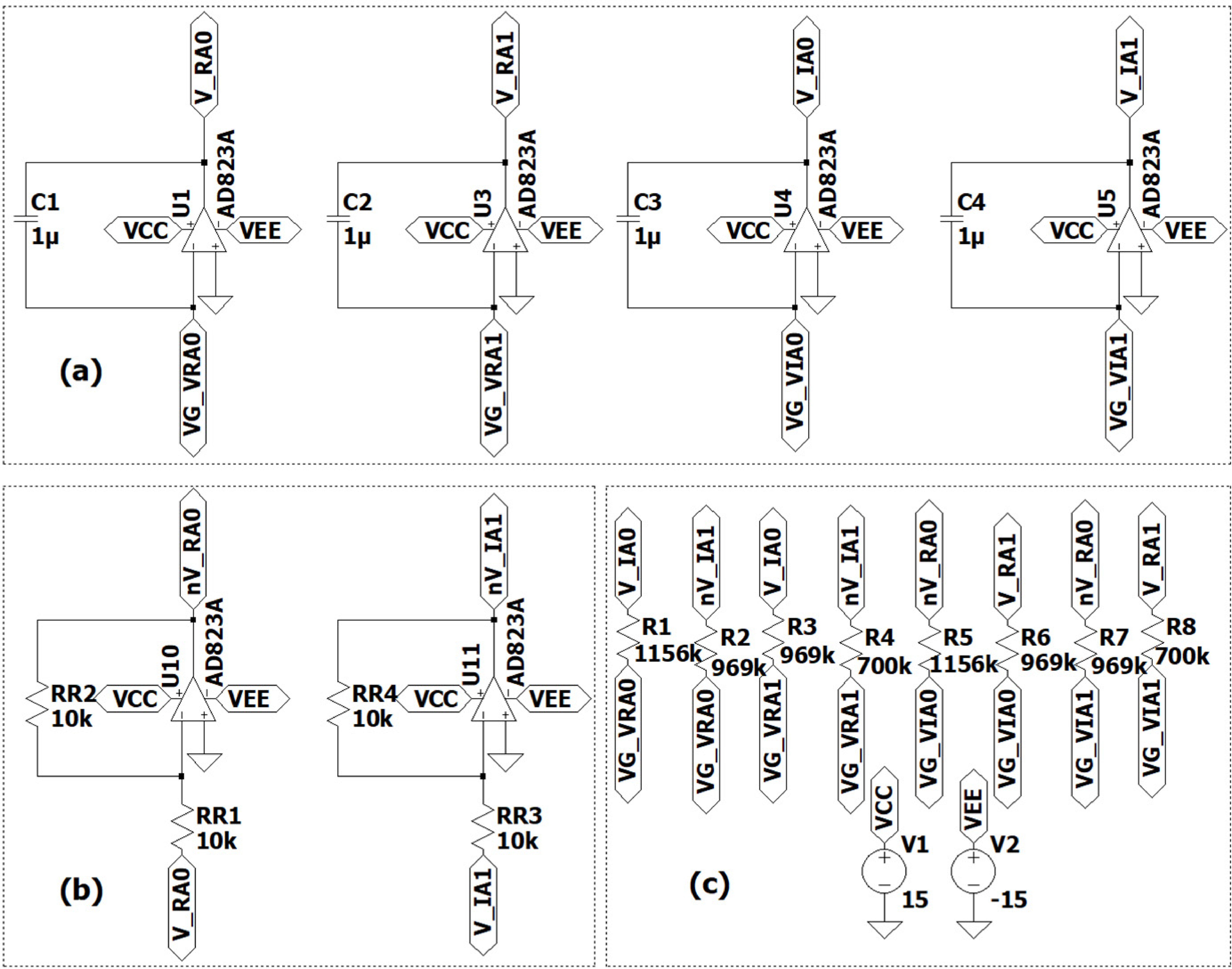
The real-valued dynamical equation derived in the previous section, \(\frac{\mathrm{d}V}{\mathrm{d}t} = M_8 V\), can be directly mapped onto an eight-node active RC network. Each state variable is assigned to a physical voltage node, and the couplings prescribed by the matrix elements \(M_{ij}\) are realized through appropriate resistive connections.
Every node is built around a multi-input inverting integrator: its non-inverting input is grounded, and the inverting input serves as a virtual-ground summation node. The output voltage \(V_i\) is fed back through a capacitor \(C\), while all coupled node voltages \(V_j\) are connected to the summation node through resistors \(R_{ij}\). Kirchhoff’s current law at the summation node yields \[C\frac{\mathrm{d}V_i}{\mathrm{d}t} = -\sum_j \frac{V_j}{R_{ij}} .\] Comparing this with the target equation \(\frac{\mathrm{d}V_i}{\mathrm{d}t} = \sum_j M_{ij} V_j\) immediately gives the component-matrix correspondence \[M_{ij} = -\frac{1}{R_{ij}C}. \label{eq:resistor95mapping}\tag{15}\] A uniform feedback capacitance \(C = 1\,\mu\mathrm{F}\) is adopted throughout to set the overall timescale.
The sign of each coupling is implemented according to the matrix element \(M_{ij}\). Negative couplings are realized by a direct resistive connection from the source node to the target integrator, because the inverting integrator intrinsically introduces a minus sign. Positive couplings require an additional sign reversal, which is accomplished by inserting a unity-gain inverting amplifier before the integrator input. Thus the entire network is constructed from only two elementary building blocks: multi-input inverting integrators and unity-gain inverting amplifiers, interconnected by appropriately chosen resistors.
3.3.2 Explicit Node Equations and Component Values↩︎
The dynamics naturally decouples into two independent sectors, labelled \(A\) and \(B\). Taking the \(A\) block as an example, we expand the state vector in the basis \((\tilde{V}_R^{A0},\tilde{V}_R^{A1},\tilde{V}_I^{A0},\tilde{V}_I^{A1})^{T}\). The corresponding real-valued dynamical matrix reads \[M_A = \begin{pmatrix} 0 & 0 & h_{00} & h_{01}\\ 0 & 0 & h_{10} & h_{11}\\ -h_{00} & -h_{01} & 0 & 0\\ -h_{10} & -h_{11} & 0 & 0 \end{pmatrix},\] with \(h_{00}=\frac{\beta}{2}-\frac{\beta}{\alpha}-\frac{1}{2}\), \(h_{01}=\frac{r}{\alpha}\), \(h_{10}=-\frac{r}{\alpha}\) and \(h_{11}=\frac{\beta}{2}+\frac{\beta}{\alpha}+\frac{1}{2}\). Expressing the node equations explicitly, \[\begin{align} \frac{\mathrm{d}}{\mathrm{d}t}\tilde{V}^{A0}_R &= h_{00}\tilde{V}^{A0}_I + \frac{r}{\alpha}\tilde{V}^{A1}_I,\notag\\[2pt] \frac{\mathrm{d}}{\mathrm{d}t}\tilde{V}^{A1}_R &= h_{11}\tilde{V}^{A1}_I - \frac{r}{\alpha}\tilde{V}^{A0}_I,\notag\\[2pt] \frac{\mathrm{d}}{\mathrm{d}t}\tilde{V}^{A0}_I &= -h_{00}\tilde{V}^{A0}_R - \frac{r}{\alpha}\tilde{V}^{A1}_R,\notag\\[2pt] \frac{\mathrm{d}}{\mathrm{d}t}\tilde{V}^{A1}_I &= -h_{11}\tilde{V}^{A1}_R + \frac{r}{\alpha}\tilde{V}^{A0}_R, \end{align}\] which uniquely determine the circuit topology. Negative coefficients correspond to direct resistive couplings, whereas positive coefficients require an additional unity-gain inverter. Since the signs of \(h_{00}\), \(h_{11}\), and \(r/\alpha\) remain unchanged over the whole parameter range, varying the purity parameter \(r\) only modifies the resistance values without altering the circuit topology.
For the \(A\) block, only three types of coupling resistors are needed: \[R_{A0}=\frac{1}{|h_{00}|C},\quad R_{\kappa}=\frac{\alpha}{rC},\quad R_{A1}=\frac{1}{|h_{11}|C}.\] The \(B\) block is constructed analogously, with the matrix entries of \(\tilde{H}_A\) replaced by the corresponding entries of \(\tilde{H}_B\) appearing in the \(B\) block of \(M_8\) in Eq. (14 ). The complete eight-node system therefore requires four unity-gain inverters.
3.3.3 Initialization and Measurement Protocol↩︎
The initial state of the circuit is prepared by mapping the theoretical purification amplitude \(W(0)=\sqrt{\rho(0)}\) onto the integrator voltages. At \(\phi=0\), \(\sqrt{\rho(0)} = \begin{pmatrix} a & b \\ b & a \end{pmatrix}\) with \(a,b=\frac{1}{2}\left(\sqrt{\frac{1+r}{2}}\pm\sqrt{\frac{1-r}{2}}\right)\). To improve the signal amplitude and reduce numerical errors, we introduce a global scaling factor \(\mathrm{amp}=10\) and set \(\upsilon_a = a\,\mathrm{amp}\), \(\upsilon_b = b\,\mathrm{amp}\). The initial voltages of the eight integrator nodes are then \[V(0) = \bigl(\upsilon_a,\upsilon_b,0,0,\; \upsilon_b,\upsilon_a,0,0\bigr)^{T},\] whose components correspond to \[(V_R^{A0},V_R^{A1},V_I^{A0},V_I^{A1},\; V_R^{B0},V_R^{B1},V_I^{B0},V_I^{B1})^{T}.\] Representative resistance values and initial voltages for several values of \(r\) are listed in Table 1.
| \(r\) | \(R_{A0}\) | \(R_{\kappa}\) | \(R_{A1}\) | \(R_{B0}\) | \(R_{B1}\) | \(a\,\mathrm{amp}\) | \(b\,\mathrm{amp}\) |
|---|---|---|---|---|---|---|---|
| 0.300 | 1996 | 6360 | 1828 | 1828 | 1996 | 6.989 | 1.073 |
| 0.500 | 1959 | 3464 | 1552 | 1552 | 1959 | 6.830 | 1.830 |
| 0.700 | 1795 | 2040 | 1186 | 1186 | 1795 | 6.546 | 2.673 |
| 0.866 | 1333 | 1155 | 800 | 800 | 1333 | 6.124 | 3.535 |
| 0.900 | 1156 | 969 | 700 | 700 | 1156 | 5.991 | 3.755 |
As an illustrative example, Fig. 1 shows the circuit implementation of the \(A\) block for \(r=0.9\); the \(B\) block has an identical structure and is omitted for clarity.
For each value of \(r\), the resistance values and initial voltages are determined from the effective dynamical matrix, and transient simulations are performed in LTspice over one complete evolution cycle \(\phi:0\rightarrow2\pi\). The circuit dynamics are solved by LTspice, while parameter sweeping, data extraction, and phase calculations are handled automatically through Python scripts.
After the simulation, the final voltages of the eight nodes are used to reconstruct the complex voltage vector \[|V_c(T)\rangle = \begin{pmatrix} V_R^{A0}(T)+\mathrm{i} V_I^{A0}(T)\\ V_R^{A1}(T)+\mathrm{i} V_I^{A1}(T)\\ V_R^{B0}(T)+\mathrm{i} V_I^{B0}(T)\\ V_R^{B1}(T)+\mathrm{i} V_I^{B1}(T) \end{pmatrix}.\] The measured overlap is \(I_{\exp} = -\langle V_c(0)|V_c(T)\rangle\). Accounting for the global scaling factor, the normalized overlap is \(I = I_{\exp}/\mathrm{amp}^{2}\), its magnitude is \(|I| = \sqrt{(\mathrm{Re}I_{\exp})^{2}+(\mathrm{Im}I_{\exp})^{2}}/\mathrm{amp}^{2}\), and the Uhlmann geometric phase is obtained as \(\Phi_U = \arg(I) = \mathrm{atan2}(\mathrm{Im}I_{\exp},\mathrm{Re}I_{\exp})\). This procedure establishes a direct experimental pathway from the measured circuit voltages to the Uhlmann geometric phase.
3.4 LTspice Simulation Results and Comparison with Theory↩︎
To validate the proposed circuit, we first examine a representative case deep in the non-trivial Uhlmann phase regime. Figure 2 shows the time evolution of the four state variables of block \(A\) at \(r=0.9\): \(\tilde{V}_R^{A0}\), \(\tilde{V}_I^{A0}\), \(\tilde{V}_R^{A1}\), and \(\tilde{V}_I^{A1}\). The LTspice simulations (blue solid lines) are compared directly with the exact theoretical solutions (red dashed lines).

After a brief initial transient (about \(1\,\mu\mathrm{s}\)) caused by the internal dynamics of the AD823A operational-amplifier macro-model, the circuit voltages quickly lock onto the prescribed initial condition and track the theoretical trajectories with high fidelity over the entire cycle. This close agreement confirms that the active RC network faithfully reproduces the Uhlmann parallel-transport dynamics at the single-trajectory level.
A more stringent test is provided by the global geometric quantities. Figure 3 summarizes the Uhlmann phase \(\Phi_U\) and the normalized overlap magnitude \(|I|\) as functions of the purity parameter \(r\), sweeping across the topological transition. The simulated data points (circles) are superimposed on the theoretical curves (dashed lines).
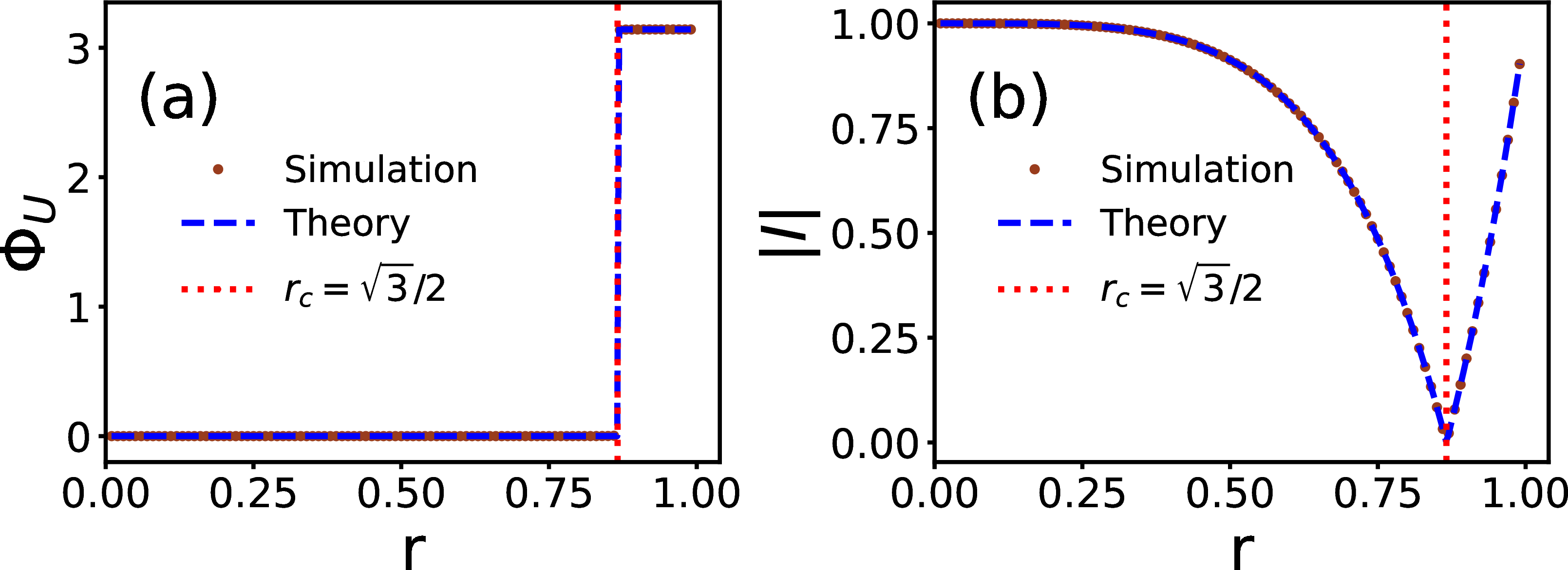
For \(r < r_c = \sqrt{3}/2\), the Uhlmann phase stays at zero; for \(r > r_c\), it jumps to \(\pi\), exactly at the critical purity predicted by the analytical formula \(\Phi_U = \arg[\cos(\pi\beta)]\) with \(\beta = 1-\sqrt{1-r^{2}}\). The overlap magnitude \(|I|\) likewise follows the theoretical expression \(|I| = |\cos(\pi\beta)|\), exhibiting a pronounced dip near \(r_c\) where the overlap vanishes. The simultaneous quantitative agreement of both quantities over the whole range of \(r\) demonstrates that the classical circuit not only reproduces the local dynamics but also captures the global topological signature of the Uhlmann phase.
Taken together, these results confirm that the proposed active RC network provides a faithful and experimentally accessible analogue of Uhlmann parallel transport, opening a practical route to investigating mixed-state geometric phases on a classical circuit platform.
4 Conclusion↩︎
We have shown that the Uhlmann parallel-transport condition for mixed states can be reformulated as a linear matrix differential equation and mapped, via vectorization, onto the admittance matrix of an active RC circuit. The resulting dynamical generator is made time-independent through a permutation and a rotating-frame transformation, and its non-Hermitian character is tamed by a real-valued decomposition, yielding a stable, purely real linear system directly realizable with operational amplifiers and resistors. LTspice simulations of the equatorial-loop model faithfully reproduce the Uhlmann geometric phase and its topological \(\pi\)-transition at the critical purity \(r_c=\sqrt{3}/2\), confirming the viability of the approach. This classical electrical-circuit platform offers an experimentally accessible route to emulating mixed-state geometric phases and may be extended to higher-dimensional or interacting systems.
5 Acknowledgments↩︎
H. G. was supported by the Quantum Science and Technology-National Science and Technology Major Project (Grant No. 2021ZD0301904) and the National Natural Science Foundation of China (Grant No. 12447216). X. Y. H. was supported by the Jiangsu Funding Program for Excellent Postdoctoral Talent (Grant No. 2023ZB611).
6 One–Cycle Overlap and Phase Invariance↩︎
We show explicitly that neither the basis permutation \(P\) nor the rotating-frame transformation \(\hat{U}(\phi)\) introduced in the main text modifies the Uhlmann geometric phase. The phase is defined by the overlap of the original vectorized purification, \[\Phi_U = \arg\!\bigl[V^\dagger(0)V(2\pi)\bigr] .\]
Step 1: permutation. Because \(P\) is a unitary matrix (\(P^\dagger P = I\)), the overlap is unchanged under the reordering \(\hat{V} = P V\): \[V^\dagger(0)V(2\pi) = \hat{V}^\dagger(0)\hat{V}(2\pi).\]
Step 2: rotating frame. The second transformation acts independently on each block, \(\hat{V}_j(\phi) = \hat{U}(\phi)\tilde{V}_j(\phi)\) with \(j=A,B\), where \(\hat{U}(\phi)\) is given by Eq. (12 ). This step removes the residual \(\phi\)-dependence from the Hamiltonians, which become \[\tilde{H}_A = \frac{\beta}{2}I + M , \quad \tilde{H}_B = -\frac{\beta}{2}I + M ,\] with \[M = \begin{pmatrix} -\dfrac{\beta}{\alpha}-\dfrac12 & \dfrac{r}{\alpha} \\[8pt] -\dfrac{r}{\alpha} & \dfrac{\beta}{\alpha}+\dfrac12 \end{pmatrix}.\] Because \(\tilde{H}_A\) and \(\tilde{H}_B\) are constant matrices, the evolution operators after one full cycle (\(\phi\) from \(0\) to \(2\pi\)) are simply \[\tilde{\mathcal{U}}_{A,B}(2\pi) = \mathrm{e}^{-\mathrm{i}2\pi \tilde{H}_{A,B}} .\]
Consider block \(A\): \[\begin{align} \tilde{\mathcal{U}}_A(2\pi) &= \mathrm{e}^{-\mathrm{i}2\pi(\frac{\beta}{2}I + M)} = \mathrm{e}^{-\mathrm{i}\pi\beta}\,\mathrm{e}^{-\mathrm{i}2\pi M} . \end{align}\] Noting that \(2\pi M = \pi(2M)\) and \((2M)^2 = I\), the second factor reduces to \[\mathrm{e}^{-\mathrm{i}\pi(2M)} = \cos(\pi)I - \mathrm{i}\sin(\pi)(2M) = -I .\] Thus \[\tilde{\mathcal{U}}_A(2\pi) = -\mathrm{e}^{-\mathrm{i}\pi\beta} I .\] An identical calculation for block \(B\) gives \[\tilde{\mathcal{U}}_B(2\pi) = -\mathrm{e}^{\mathrm{i}\pi\beta} I .\]
The initial purification is \(\sqrt{\rho} = \begin{pmatrix} a & b \\ b & a \end{pmatrix}\) with \(a,b = \frac{1}{2}\bigl(\sqrt{\frac{1+r}{2}} \pm \sqrt{\frac{1-r}{2}}\bigr)\). Its row-vectorization yields \(V(0) = (a,b,b,a)^T\), which after permutation decomposes as \[\hat{V}_A(0) = \begin{pmatrix} a \\ b \end{pmatrix},\quad \hat{V}_B(0) = \begin{pmatrix} b \\ a \end{pmatrix}.\] Using \(V^\dagger V = \operatorname{Tr}(W^\dagger W) = \operatorname{Tr}(\rho) = 1\), we have \(2(a^2+b^2)=1\), hence \(a^2+b^2 = 1/2\) and \[\hat{V}_A^\dagger\hat{V}_A = \hat{V}_B^\dagger\hat{V}_B = \frac{1}{2} .\] Unitarity of \(\hat{U}(\phi)\) preserves these norms, \[\tilde{V}_A^\dagger\tilde{V}_A = \tilde{V}_B^\dagger\tilde{V}_B = \frac{1}{2} .\] The boundary values of \(\hat{U}(\phi)\) are \(\hat{U}(0) = I\) and \(\hat{U}(2\pi) = \begin{pmatrix} \mathrm{e}^{-\mathrm{i}\pi} & 0 \\ 0 & \mathrm{e}^{\mathrm{i}\pi} \end{pmatrix} = -I\). Consequently, at the end of the cycle, \[\hat{V}_j(2\pi) = \hat{U}(2\pi)\tilde{V}_j(2\pi) = -\tilde{V}_j(2\pi) .\] We can now evaluate the overlap, inserting this sign together with the evolution operators: \[\begin{align} &V^\dagger(0)V(2\pi) = \hat{V}^\dagger(0)\hat{V}(2\pi) \notag\\ =& \sum_{j=A,B} \tilde{V}_j^\dagger(0)\,\bigl[-\tilde{\mathcal{U}}_j(2\pi)\bigr]\, \tilde{V}_j(0) \notag\\ =& \tilde{V}_A^\dagger(0)\bigl[-(-\mathrm{e}^{-\mathrm{i}\pi\beta}I)\bigr]\tilde{V}_A(0) + \tilde{V}_B^\dagger(0)\bigl[-(-\mathrm{e}^{\mathrm{i}\pi\beta}I)\bigr]\tilde{V}_B(0) \notag\\ =& \cos(\pi\beta). \end{align}\] The two minus signs cancel, leaving exactly the overlap one obtains from the original Uhlmann parallel-transport theory. Therefore the Uhlmann phase \[\Phi_U = \arg\!\bigl[\cos(\pi\beta)\bigr]\] is unchanged by the auxiliary transformations. It exhibits the topological \(\pi\)-jump at \(\beta = 1/2\), i.e.at the critical purity \(r_c = \sqrt{3}/2\).