1 Introduction and summary of results↩︎

Euler [1] derived the following expression for the product of all natural numbers \[\label{Euler-prod} P= 1\cdot 2 \cdot 3\cdot 4\cdot 5\cdot 6\cdot 7\cdots = \sqrt{2\pi},\tag{1}\] long before regularized infinite products were put on firm ground within the so-called zeta-regularization technique, which is based on analytical continuation (see [2]–[5] for historical accounts). Nowadays, zeta-regularized infinite products are used in many fields. In the physics literature, they are often referred to as renormalized products. A prominent instance consists in the determinants, i.e., products of all eigenvalues, of various operators arising in geometry, quantum mechanics and quantum field theory (see e.g. [6]–[15], and [16]–[18] for overviews).

In view of (1 ), it is natural to wonder whether one can make sense of the product \({\mathit{\Pi}}\) of all natural primes. This question has seemingly been first asked by Soulé [10]. It is made difficult by the fact that the prime zeta function \({\mathcal{P}}(s)\) has a natural boundary along the imaginary axis. It is therefore not analytic in a neighborhood of the origin, which is required for the applicability of the zeta-regularization approach, expressing \({\mathit{\Pi}}\) in terms of \({\mathcal{P}}'(0)\). Muñoz García and Pérez-Marco [19], [20] found a way to overcome this problem and evaluated the product of natural primes: \[\label{Soule-prod} {\mathit{\Pi}}= 2 \cdot 3\cdot 5\cdot 7 \cdot 11 \cdot 13\cdots = (2\pi)^2.\tag{2}\] The power-law relation \[{\mathit{\Pi}}=P^4 \label{qpnat}\tag{3}\] between the two regularized products, a curiosity at first sight, actually extends to all number fields for which we succeeded in computing the analogues of (1 ) and (2 ) (see (10 )).

The interest in the derivation of (2 ) goes far beyond the realm of number theory. A variety of situations can indeed be found in the physics literature, where the zeta-regularization technique had to be adapted or generalized, because the relevant zeta function either does not have a meromorphic continuation, or is not analytic in a neighborhood of \(s=0\), or has a natural boundary. The quantum mechanics of one particle in a one or two-dimensional potential provides explicit examples where the spectral zeta functions may have poles and branch cuts of any order in the \(s\) plane, at positions depending on model parameters (see e.g. [21], [22]). More generally, natural boundaries have also been met in statistical mechanics [23], [24], in gauge theories [25], in scattering amplitudes [26]. It was recently advocated [25], [27], [28] that resurgence theory leads to a new form of unique continuation, beyond analytic continuation.

The formula (2 ) suggests seeking other prime analogues of classical divergent products and sums admitting a zeta-regularization procedure. Two especially popular zeta-regularized sums, also going back to Euler, are \[\begin{align} \tag{4} 1+2+3+4+5+\cdots &=& \zeta(-1)= -\frac{1}{12},\\ \tag{5} 1^3+2^3+3^3+4^3+\cdots &=& \zeta(-3)= \frac{1}{120}. \end{align}\] The sum of natural numbers (4 ) is the most famous zeta-regularized value, endlessly discussed by science lovers astonished by the fact that this sum is finite and negative. The sum (5 ) is the first zeta-regularized value experimentally measured. It appeared in the Casimir formula [29] for the force between two conducting plates in vacuum (see [30] for very recent work on the Casimir effect, and [31] for an overview).

The first challenge we address here is to make sense of the sum of all primes, thereby providing the prime analogue of (4 ). This task looks formidable, because it involves \({\mathcal{P}}(-1)\), and \(s=-1\) sits at a finite distance beyond the natural boundary. We then extend the products (1 ) and (2 ) to the regularized products of integers and primes in the nine imaginary quadratic fields where integers have a unique factorization into primes. Hopefully, the techniques developed here in a number-theoretic context can be applied to some of the physically interesting problems mentioned above.

The present paper is organized as follows. In section 2, we consider products of natural integers and primes. We recall the modern derivation of (1 ) in section 2.1, whereas in section 2.2 we recall the derivation of (2 ) by Muñoz García and Pérez-Marco and provide further results on the prime zeta function. The main novel part on natural primes resides in section 3, which contains a detailed heuristic derivation of the regularized sum of primes, yielding \[\begin{align} {\mathcal{P}}(-1) &=& 2+3+5+7+11+13+\cdots \nonumber\\ &=&\frac{5}{2}+\sum_{n\ge1}\frac{\mu(n)}{n}\log\frac{n!(\e/n)^n\zeta(n+1)}{\sqrt{2\pi n}} =2.925\,292\,456\dots \label{pmun} \end{align}\tag{6}\] The non-trivial part of the computation involving the regularization of divergent sums gave the simple rational number \(5/2\), while the complicated sum appearing on the right-hand side of the above expression is convergent, and in this sense trivial.

The remainder of the paper is devoted to the regularization of the products of integers and primes in some algebraic extensions of the rationals, namely imaginary quadratic fields where integers have a unique factorization into primes. Gauss conjectured that there are exactly nine such quadratic fields with class number one (see [32]–[36] for information about this and other class number problems going back to Gauss). Sections 4 and 5 are devoted to detailed heuristic computations à la Euler, inspired by [19], [20], of the regularized infinite products of Gauss integers \({\mathbb{Z}}[{\rm i}]\) and Eisenstein integers \({\mathbb{Z}}[\omega]\), with \(\omega=(-1+{\rm i}\sqrt3)/2=\e^{2\pi{\rm i}/3}\), and of the associated primes. These two well-known cases are, in several regards, the most obvious generalizations of the natural integers and primes. They are related to the two simplest planar quantum billiards whose spectra are integrable, namely the square and the equilateral triangle [37], [38]. They also play a part in recent developments in cosmology (see [39] and references therein).

For Gauss integers (see section 4), we find that the product \(P_4\) of all non-zero Gauss integers and the product \({\mathit{\Pi}}_4\) of all Gauss primes obeys \[{\left\vert{\mathit{\Pi}}_4\right\vert}={\left\vert P_4\right\vert}^8. \label{qp4}\tag{7}\] For Eisenstein integers (see section 5), we obtain similarly \[{\left\vert{\mathit{\Pi}}_3\right\vert}={\left\vert P_3\right\vert}^{12}. \label{qp3}\tag{8}\] In section 6 we extend the computation of the products of integers and primes to the remaining seven imaginary quadratic fields whose rings of integers have unique factorization. The absolute discriminants of these fields are the Heegner numbers \(\Delta=7\), 8, 11, 19, 43, 67, and 163. There, we find \[{\left\vert{\mathit{\Pi}}_\Delta\right\vert}={\left\vert P_\Delta\right\vert}^4. \label{qpp}\tag{9}\]

All the above results concerning quadratic number fields can be summarized into the following universal formula \[{\left\vert{\mathit{\Pi}}_\Delta\right\vert}={\left\vert P_\Delta\right\vert}^{2w_\Delta}, \label{qpgal}\tag{10}\] where the exponent \(2w_\Delta\) is twice the number of units, namely 12 for Eisenstein integers (see (8 )), 8 for Gauss integers (see (7 )), and 4 for the other imaginary quadratic fields (see (9 )), just as for natural integers and primes (see (3 )). Whether the formula (10 ) holds for more general algebraic number fields remains an open question. The most natural extension is to real quadratic fields \({\mathbb{Q}}\big(\sqrt{d}\big)\), where \(d\) is a positive squarefree integer. The conjecture by Gauss that there are infinitely many such real quadratic fields with class number one is still open.

Besides the present number-theoretic context, a great deal of regularized products of natural integers, such as those associated with periodic, aperiodic, and random sequences, are the subject of current work that will be reported elsewhere [40].

2 Products of natural integers and primes↩︎

2.1 Product of natural integers↩︎

The product of all natural integers, \[P=\prod_{n\ge1}n, \label{pnatural}\tag{11}\] can be regularized by relating it to the Riemann zeta function \[\zeta(s)=\sum_{n\ge1}n^{-s}=\prod_{p\;{\mathop{\rm prime}}}(1-p^{-s})^{-1}. \label{zeta}\tag{12}\] We have indeed formally \[P=\exp\sum_{n\ge1}\log n=\exp\left(-\zeta'(0)\right). \label{plog}\tag{13}\] This expression is the gist of the zeta-regularization, consisting in regularizing divergent products such as (11 ) by means of analytic continuation. The series and product entering (12 ) converge for \(\mathop{\rm Re}(s)>1\) and can be analytically continued to a meromorphic function in the whole complex \(s\)-plane, with a simple pole with unit residue at \(s=1\). In particular, \(\zeta(s)\) is analytic in a neighborhood of \(s=0\), with \[\zeta(0)=-\frac{1}{2},\qquad\zeta'(0)=-\frac{1}{2}\log 2\pi. \label{z0}\tag{14}\] Inserting the second of these expressions into (13 ), we recover Euler’s expression (1 ).

2.2 Product of natural primes↩︎

In the same vein, the product of all natural primes, \[{\mathit{\Pi}}=\prod_{p\;{\mathop{\rm prime}}}p, \label{qnatural}\tag{15}\] is formally given by \[{\mathit{\Pi}}=\exp\left(-{\mathcal{P}}'(0)\right), \label{qlog}\tag{16}\] where \({\mathcal{P}}(s)\) is the prime zeta function (see e.g. [41]–[44]): \[{\mathcal{P}}(s)=\sum_{p\;{\mathop{\rm prime}}}p^{-s}. \label{zdef}\tag{17}\]

As recalled above, at variance with (13 ), the usage of (16 ) is compromised by the fact that \({\mathcal{P}}(s)\) has a natural boundary along the imaginary axis and is therefore not analytic in a neighborhood of \(s=0\). This obstacle has been circumvented by Muñoz García and Pérez-Marco [19], [20]. Their heuristic derivation [19] starts with the Artin-Hasse identity for the exponential function, \[\e^x=\prod_{n\ge1}(1-x^n)^{-\mu(n)/n}, \label{ah}\tag{18}\] where \(\mu(n)\) is the Möbius function: \[\mu(n)=\left\{ \begin{array}{cl} (-1)^k & if n is the product of k distinct primes,\\ 0 &else. \end{array} \right.\label{mudef}\tag{19}\] Combining (17 ) and (18 ), we obtain \[\begin{align} \exp({\mathcal{P}}(s)) &=&\prod_{p\;{\mathop{\rm prime}}}\exp(p^{-s}) \nonumber\\ &=&\prod_{p\;{\mathop{\rm prime}}}\prod_{n\ge1}(1-p^{-ns})^{-\mu(n)/n} \nonumber\\ &=&\prod_{n\ge1}\prod_{p\;{\mathop{\rm prime}}}(1-p^{-ns})^{-\mu(n)/n} \nonumber\\ &=&\prod_{n\ge1}\zeta(ns)^{\mu(n)/n}\,. \label{ezprod} \end{align}\tag{20}\] Taking logarithms of both sides yields \[{\mathcal{P}}(s)=\sum_{n\ge1}\frac{\mu(n)}{n}\log\zeta(ns). \label{pmobius}\tag{21}\] This expression was first established [41]–[44] by applying the Möbius inversion formula to the identity \[\log\zeta(s)=\sum_{n\ge1}\frac{{\mathcal{P}}(ns)}{n},\] that can be derived from the Euler product formula (12 ). The expression (21 ) shows that the prime zeta function has a natural boundary along the imaginary axis. The zeros of the Riemann zeta function at \(s_n=1/2+{\rm i}t_n\) along the critical line indeed generate logarithmic branch cuts accumulating along the whole imaginary axis. The function \({\mathcal{P}}(s)\) also has an infinite sequence of logarithmic branch cuts along the real axis accumulating at the origin (see figure 1). These singularities are located at \(s=1/k\) whenever \(\mu(k)\ne0\), i.e., \(k\) is squarefree. More specifically, there are upward singularities at \(s=1/k\) whenever \(\mu(k)=1\), i.e., \(k=1\), 6, 10, 14, 15... and downward singularities at \(s=1/k\) whenever \(\mu(k)=-1\), i.e., \(k=2\), 3, 5, 7, 11...

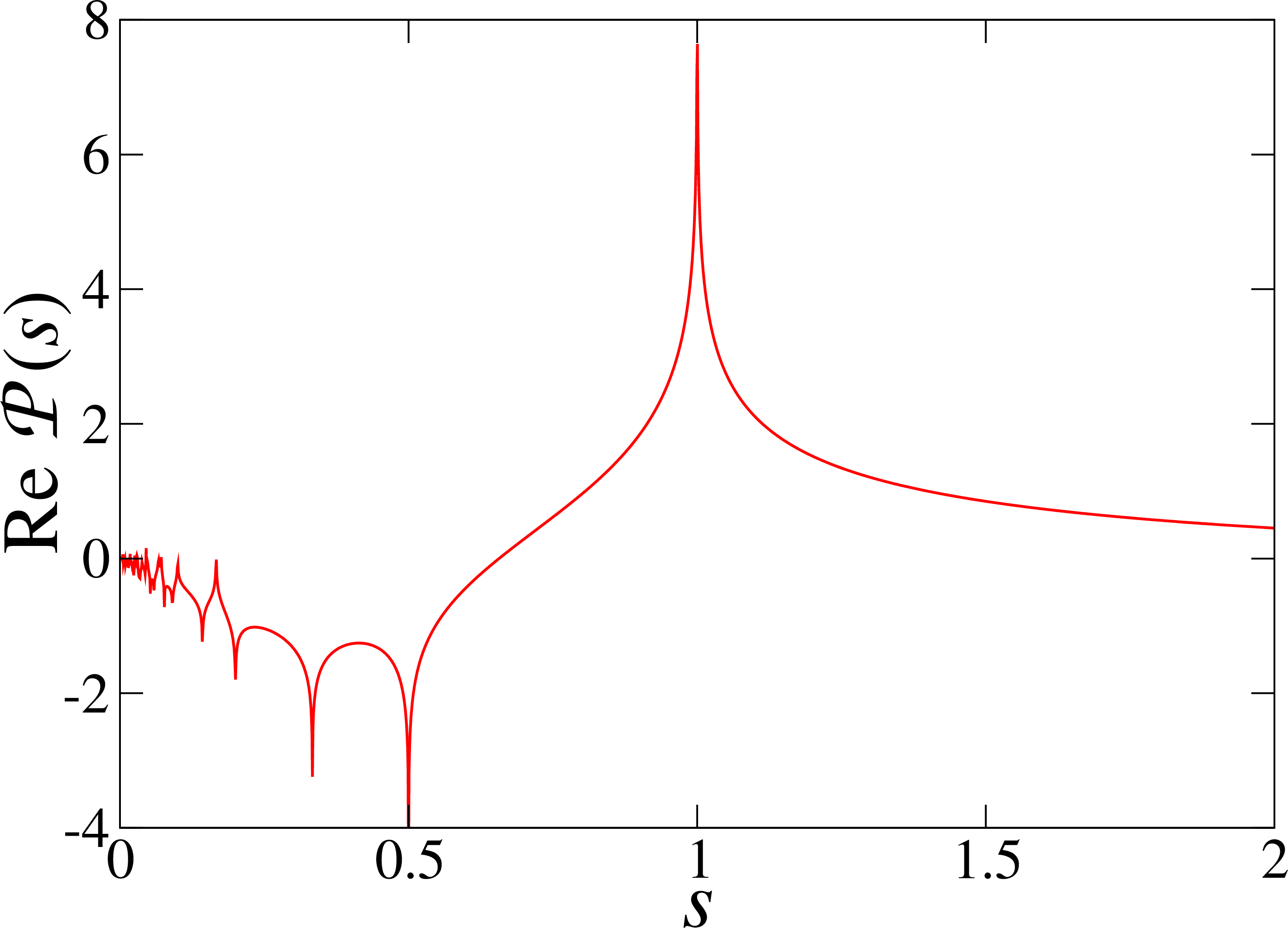
The expression (21 ) can be used to evaluate regularized values of \({\mathcal{P}}\) and its derivatives at \(s=0\). In this approach, sums involving the Möbius function are consistently evaluated by means of the zeta-regularization scheme, using \[\label{mu-z} M(s)=\sum_{n\ge1}\mu(n)\,n^{-s}=\frac{1}{\zeta(s)}\,.\tag{22}\] In the simplest case of \({\mathcal{P}}(0)\), (21 ) yields \[{\mathcal{P}}(0)=\log\zeta(0)\sum_{n\ge1}\frac{\mu(n)}{n},\] where the sum over \(n\) evaluates to \(M(1)=1/\zeta(1)=0\), so that \[{\mathcal{P}}(0)=0.\] The value of \({\mathcal{P}}'(0)\) is of special interest as it enters (16 ). We have \[\label{Ps-1} {\mathcal{P}}'(s)=\sum_{n\ge1}\mu(n)\frac{\zeta'(ns)}{\zeta(ns)},\tag{23}\] and in particular \[{\mathcal{P}}'(0)=\frac{\zeta'(0)}{\zeta(0)}\sum_{n\ge1}\mu(n). \label{zpz}\tag{24}\] The sum evaluates to \(M(0)=1/\zeta(0)\). We thus obtain, using (14 ), \[{\mathcal{P}}'(0)=\frac{\zeta'(0)}{\zeta(0)^2}=-2\log(2\pi), \label{zp}\tag{25}\] and so, using (16 ), we arrive at (2 ), the central result of [19], [20].

The same approach applies to higher-order derivatives as well. In the case of \({\mathcal{P}}''(0)\), taking the derivative of (23 ) and specializing to \(s=0\), we arrive at \[{\mathcal{P}}''(0)=\left(\frac{\zeta''(0)}{\zeta(0)}-\left[\frac{\zeta'(0)}{\zeta(0)}\right]^2\right) \sum_{n\ge1}n\mu(n).\] The sum evaluates to \(M(-1)=1/\zeta(-1)=-12\). Using the expression \[\zeta''(0)=\frac{\gamma^2}{2}+\gamma_1-\frac{\pi^2}{24}-\frac{[\log(2\pi)]^2}{2}, \label{z0-2}\tag{26}\] following from the reflection formula (38 ), we obtain \[{\mathcal{P}}''(0)=12\gamma^2+24\gamma_1-\pi^2. \label{P0-2}\tag{27}\] The constants \[\gamma=\gamma_0=0.577\,215\,664\dots, \qquad \gamma_1=-0.072\,815\,845\dots\] are the Euler and Stieltjes constants appearing in the Laurent series expansion of the Riemann zeta function \[\zeta(1+s)=\frac{1}{s}+ \sum_{n\geq 0} \frac{(-1)^n}{n!}\, \gamma_n s^n. \label{z-exp}\tag{28}\] A similar computation yields \({\mathcal{P}}'''(0)=\infty\). This quantity is indeed proportional to \(M(2)=1/\zeta(-2)\), and \(\zeta(-2)=0\).

Although evaluating the regularized product \({\mathit{\Pi}}\) of all primes proved to be a challenging problem resolved only recently, some infinite products involving primes are easy to regularize. For instance, the Euler product formula (12 ) gives \[\begin{align} \prod_{p\;{\mathop{\rm prime}}}\big(1-p^{2k}\big)=\frac{1}{\zeta(-2k)}=\infty, \nonumber\\ \prod_{p\;{\mathop{\rm prime}}}\big(1-p^{2k-1}\big)=\frac{1}{\zeta(1-2k)}= -\frac{2k}{B_{2k}} \end{align}\] for any integer \(k\ge1\) (see (34 )). Specializing these formulas to \(k=1\) we obtain \[\prod_{p\;{\mathop{\rm prime}}}\big(1-p^{2}\big)=\infty, \quad \prod_{p\;{\mathop{\rm prime}}}(1-p\big)=-12.\] This yields formally \[\prod_{p\;{\mathop{\rm prime}}}(1+p)=\infty,\] and suggests that \[\prod_{p\;{\mathop{\rm prime}}}(p+x)\] has no natural regularized expression. Such an expression would be a prime analogue of the Lerch formula [45], [46] (see (49 )) \[\label{Lerch:prod} \prod_{n\ge0}(n+x)=\frac{\sqrt{2\pi}}{\Gamma(x)},\tag{29}\] which is itself a renormalized avatar of the Weierstrass product formula \[\frac{1}{\Gamma(x)}=x\,\e^{\gamma x}\prod_{n\ge1}(1+x/n)\e^{-x/n}.\]

Finally, we mention that the product \[\prod_{n\ge1}n^n=\exp(-\zeta'(-1))=1.179\,889\,917\dots \label{nn}\tag{30}\] admits a prime analogue, \[\prod_{p\;{\mathop{\rm prime}}}p^p=\exp(-{\mathcal{P}}'(-1)), \label{pp}\tag{31}\] where \[\label{P-1} {\mathcal{P}}'(-1)=\sum_{n\ge1}\mu(n)\frac{\zeta'(-n)}{\zeta(-n)}.\tag{32}\] The regularized values of this quantity could be determined along the lines of section 3.

3 Sums of natural integers and primes↩︎

Regularized sums of powers of natural numbers are more popular than regularized products. The well-known examples like (4 ) and (5 ) are special cases of the general Euler’s formula [47] \[\label{z-k} \sum_{n\ge1}n^m=\zeta(-m),\tag{33}\] expressing the regularized sums of powers of natural numbers in terms of the Bernoulli numbers, namely \[\zeta(-2k)=0,\quad\zeta(1-2k)=-\frac{B_{2k}}{2k}\qquad(k\ge1). \label{zetaint}\tag{34}\]

In view of the above, it is quite natural to consider the zeta-regularized sums of powers of primes \[{\mathcal{P}}(-m)=\sum_{p\;{\mathop{\rm prime}}}p^m,\] for which the formula (21 ) yields \[{\mathcal{P}}(-m)=\sum_{n\ge1}\frac{\mu(n)}{n}\log\zeta(-mn). \label{pm}\tag{35}\]

Investigating the above series is a far more formidable task than evaluating the regularized product of all primes. We recall that the prime zeta function has a natural boundary along the imaginary axis. The regularized product of all primes involves \({\mathcal{P}}'(0)\), where the origin sits on the natural boundary, whereas the regularized sums of powers of primes involve the values of \({\mathcal{P}}(s)\) at \(s=-m\), at a finite distance beyond the natural boundary.

The famous quote by the physicist Lev Landau, reproduced above, was made in connection to the Goldbach conjecture asserting that every even natural number is the sum of two prime numbers. Regularizing divergent sums is admittedly a different story. Finding an application, either in Physics or elsewhere, of \({\mathcal{P}}(-1)\), or of another \({\mathcal{P}}(-m)\), would be amusing. One should keep in mind that more than two hundred years separate the determination of \(\zeta(-3)\) by Euler (see (5 )) and the measurement of the Casimir effect, involving \(\zeta(-3)\).

We now explain how to make sense of the formula (35 ) in the first case of interest, namely the sum of all primes, \[{\mathcal{P}}(-1)=\sum_{p\;{\mathop{\rm prime}}}p.\] Setting \(m=1\) in (35 ), and taking the real parts of the logarithms, as we expect the regularized value of \({\mathcal{P}}(-1)\) to be real, we obtain \[{\mathcal{P}}(-1)=\sum_{n\ge1}\frac{\mu(n)}{n}\log{\left\vert\zeta(-n)\right\vert}.\] The Riemann zeta function vanishes at even negative integers (see (34 )), so that we rather consider \[{\mathcal{P}}(-1+\varepsilon)=\sum_{n\ge1}\frac{\mu(n)}{n}\log{\left\vert\zeta(-n+n\varepsilon)\right\vert}.\] To linear order in \(\varepsilon\), we get \[{\mathcal{P}}(-1+\varepsilon)\approx\sum_{n\;{\mathop{\rm odd}}}\frac{\mu(n)}{n}\log{\left\vert\zeta(-n)\right\vert} +\sum_{n\;{\mathop{\rm even}}}\frac{\mu(n)}{n}\log{\left\vert n\varepsilon\zeta'(-n)\right\vert}, \label{peps}\tag{36}\] and have therefore to deal separately with odd and even values of \(n\). We introduce the Dirichlet series \[M_{\mathop{\rm odd}}(s)=\sum_{n\;{\mathop{\rm odd}}}\mu(n)\,n^{-s},\quad M_{\mathop{\rm even}}(s)=\sum_{n\;{\mathop{\rm even}}}\mu(n)\,n^{-s},\] which can be related to \(M(s)\) introduced in (22 ) as follows. First, we have the sum rule \(M_{\mathop{\rm odd}}(s)+M_{\mathop{\rm even}}(s)=M(s)=1/\zeta(s)\). Second, the definition (19 ) of the Möbius function implies \[\mu(2n)=\left\{ \begin{array}{cl} -\mu(n) & (n odd),\\ 0 &(n even), \end{array}\right.\] so that \(M_{\mathop{\rm even}}(s)=-M_{\mathop{\rm odd}}(s)/2^s\). We thus obtain \[M_{\mathop{\rm odd}}(s)=\frac{2^s}{(2^s-1)\zeta(s)},\quad M_{\mathop{\rm even}}(s)=-\frac{1}{(2^s-1)\zeta(s)}. \label{mome}\tag{37}\] The terms proportional to \(\log{\left\vert\varepsilon\right\vert}\) in (36 ) sum up to \(M_{\mathop{\rm even}}(1)=0\) obtained by specializing \(M_{\mathop{\rm even}}(s)\) to \(s=1\) and recalling that \(\zeta(s)\) has a pole to \(s=1\). Therefore (36 ) has a well-defined limit \[{\mathcal{P}}(-1)=\sum_{n\;{\mathop{\rm odd}}}\frac{\mu(n)}{n}\log{\left\vert\zeta(-n)\right\vert} +\sum_{n\;{\mathop{\rm even}}}\frac{\mu(n)}{n}\log{\left\vert n\zeta'(-n)\right\vert}.\] The reflection formula for the Riemann zeta function \[\zeta(1-s)=2(2\pi)^{-s}\cos\frac{\pi s}{2}\Gamma(s)\zeta(s) \label{zetarefl}\tag{38}\] yields \[\begin{array}{ll} {\left\vert\zeta(-n)\right\vert}=\displaystyle{\displaystyle n!\,\zeta(n+1)\over\displaystyle\pi(2\pi)^n} & (n odd),\\ {\left\vert n\zeta'(-n)\right\vert}=\displaystyle{\displaystyle n\,n!\,\zeta(n+1)\over\displaystyle 2(2\pi)^n} \quad & (n even). \end{array}\] Both expressions share the common leading asymptotic behavior \((n/(2\pi\e))^n\). The corresponding regularized sum reads \[\sum_{n\ge1}\mu(n)(\log n-\log(2\pi)-1)=2,\] where we have used \[\sum_{n\ge1}\mu(n)=\frac{1}{\zeta(0)}=-2,\quad \sum_{n\ge1}\mu(n)\log n=\frac{\zeta'(0)}{\zeta(0)^2}=-2\log(2\pi).\] At this stage, we are left with \[{\mathcal{P}}(-1)=2+{\mathcal{P}}_{\mathop{\rm odd}}+{\mathcal{P}}_{\mathop{\rm even}},\] with \[\begin{align} {\mathcal{P}}_{\mathop{\rm odd}}=\sum_{n\;{\mathop{\rm odd}}}\frac{\mu(n)}{n}\log\frac{n!(\e/n)^n\zeta(n+1)}{\pi}\,, \nonumber\\ {\mathcal{P}}_{\mathop{\rm even}}=\sum_{n\;{\mathop{\rm even}}}\frac{\mu(n)}{n}\log\frac{n\,n!(\e/n)^n\zeta(n+1)}{2}\,. \end{align}\] The above sums are still divergent. The asymptotic behaviors of the arguments of the logarithms are indeed respectively \(\sqrt{2n/\pi}\) and \(\sqrt{\pi n^3/2}\). The corresponding regularized sums read \[\sum_{n\;{\mathop{\rm odd}}}\frac{\mu(n)}{n}\,\frac{\log(2n/\pi)}{2}=-1,\quad \sum_{n\;{\mathop{\rm even}}}\frac{\mu(n)}{n}\,\frac{\log(\pi n^3/2)}{2}=\frac{3}{2},\] where we have used \[\begin{align} &&\sum_{n\;{\mathop{\rm odd}}}\frac{\mu(n)}{n}=M_{\mathop{\rm odd}}(1)=0,\quad \sum_{n\;{\mathop{\rm odd}}}\frac{\mu(n)}{n}\,\log n=-M_{\mathop{\rm odd}}'(1)=-2, \nonumber\\ &&\sum_{n\;{\mathop{\rm even}}}\frac{\mu(n)}{n}=M_{\mathop{\rm even}}(1)=0,\quad \sum_{n\;{\mathop{\rm even}}}\frac{\mu(n)}{n}\,\log n=-M_{\mathop{\rm even}}'(1)=1. \nonumber\\ \end{align}\] Putting everything together, we arrive at our final expression, \[{\mathcal{P}}(-1)=\frac{5}{2}+\sum_{n\ge1}\frac{\mu(n)}{n}\log\frac{n!(\e/n)^n\zeta(n+1)}{\sqrt{2\pi n}}, \label{punana}\tag{39}\] announced in (6 ). The series is convergent and sums to \(0.425\,292\,456\dots\), and so \[{\mathcal{P}}(-1)=2.925\,292\,456\dots \label{punnum}\tag{40}\] Regularized values of \({\mathcal{P}}(-m)\) for higher integers \(m\) could be evaluated along the lines of the above derivation.

4 Gauss integers and primes↩︎

Gauss integers form the ring \({\mathbb{Z}}[{\rm i}]\). They can be viewed as the vertices of the square lattice, of the form \(z=a+b{\rm i}\), where \(a\) and \(b\) are usual integers, and so \({\left\vert z\right\vert}^2=a^2+b^2\).

4.1 Product of Gauss integers↩︎

The product of all Gauss integers is \[P_4=\prod_{(a,b)\ne(0,0)}(a+b{\rm i}). \label{p4def}\tag{41}\] The subscript \(4\) in \(P_4\) and other functions reflects the identity \({\rm i}^4=1\). The Heeger number of the Gauss number field \({\mathbb{Q}}({\rm i})\) is \(4\), and this interpretation extends to all other imaginary quadratic fields with unique factorization.

The ring \({\mathbb{Z}}[{\rm i}]\) has 4 units, namely \(\pm 1\) and \(\pm {\rm i}\). It is invariant under multiplication by \({\rm i}\). Therefore, assigning a meaning to the phase of \(P_4\) is problematic, and we limit ourselves to \[{\left\vert P_4\right\vert}^2=\prod_{(a,b)\ne(0,0)}(a^2+b^2). \label{p42def}\tag{42}\] The corresponding Dedekind zeta function, \[\zeta_4(s)=\sum_{(a,b)\ne(0,0)}(a^2+b^2)^{-s}, \label{z42def}\tag{43}\] is such that \[{\left\vert P_4\right\vert}^2=\exp\left(-\zeta_4'(0)\right). \label{p42}\tag{44}\] The theory of Dedekind zeta functions is exposed in detail in [48]–[50] for the cases of \({\mathbb{Z}}[{\rm i}]\) and \({\mathbb{Z}}[\omega]\), considered in sections 4 and 5. In the present situation, we have \[\zeta_4(s)=4\zeta(s)L_4(s), \label{z4factor}\tag{45}\] where \(\zeta(s)\) is the Riemann zeta function, and \[L_4(s)=\sum_{n\ge1}\chi_4(n)\,n^{-s}\] is the Dirichlet \(L\)-function associated with the Dirichlet character \(\chi_4\), i..e, the multiplicative function of \(n \mathop{\rm mod}4\) such that \[\chi_4(0)=0,\quad \chi_4(1)=1,\quad \chi_4(2)=0,\quad \chi_4(3)=-1. \label{chi4def}\tag{46}\] This \(L\)-function reads explicitly \[\begin{align} L_4(s) &=&\sum_{m\ge0}\left((4m+1)^{-s}-(4m+3)^{-s}\right) \nonumber\\ &=&\frac{\zeta(s,1/4)-\zeta(s,3/4)}{4^s}, \label{l4h} \end{align}\tag{47}\] in terms of the Hurwitz zeta function \[\zeta(s,x)=\sum_{m\ge0}(m+x)^{-s}. \label{hurwitz}\tag{48}\] The analytic structure of the latter function is similar to that of the Riemann zeta function, which is recovered as \(\zeta(s)=\zeta(s,1)\). In particular [49] \[\zeta(0,x)=\frac{1}{2}-x,\qquad\zeta'(0,x)=\log\frac{\Gamma(x)}{\sqrt{2\pi}}\,. \label{z0x}\tag{49}\] The second expression, and the ensuing regularized infinite product (29 ), are known as the Lerch formula [45], [46]. We also mention that \(L_4(s)\) has an Euler product representation of the form \[L_4(s)=\prod_{p\;{\mathop{\rm prime}}\ne2}(1-\chi_4(p)\,p^{-s})^{-1},\] i.e., explicitly \[L_4(s)=\frac{\zeta_{4,1}(s)\zeta_{4,3}(2s)}{\zeta_{4,3}(s)}, \label{l4zz}\tag{50}\] in terms of the partial prime zeta functions \[\begin{align} \zeta_{4,1}(s)&=&\prod_{p\;{\mathop{\rm prime}}=1\mathop{\rm mod}4}(1-p^{-s})^{-1}, \nonumber\\ \zeta_{4,3}(s)&=&\prod_{p\;{\mathop{\rm prime}}=3\mathop{\rm mod}4}(1-p^{-s})^{-1}, \label{z4143def} \end{align}\tag{51}\] which obey \[\zeta_{4,1}(s)\zeta_{4,3}(s)=(1-2^{-s})\zeta(s). \label{z4143z}\tag{52}\] Using (45 ) and (47 ), together with (14 ) and (49 ), we obtain \[\begin{align} &&L_4(0)=\frac{1}{2},\qquad L'_4(0)=\log\frac{\Gamma(1/4)}{2\Gamma(3/4)}, \tag{53} \\ &&\zeta_4(0)=-1,\qquad \zeta'_4(0)=\log\frac{2\Gamma(3/4)^2}{\pi\Gamma(1/4)^2}. \tag{54} \end{align}\] The value of \(\zeta_4(0)\) can be interpreted as counting negatively the point \((0,0)\) that is excluded from the product (42 ) and the sum (43 ). Finally, (44 ) yields \[{\left\vert P_4\right\vert}^2=\frac{\pi\Gamma(1/4)^2}{2\Gamma(3/4)^2}=\frac{\Gamma(1/4)^4}{4\pi}=13.750\,371\,636\dots \label{p4res}\tag{55}\]

4.2 Product of Gauss primes↩︎

The product of all Gauss primes, \[{\mathit{\Pi}}_4=\prod_{a+b{\rm i}\;{\mathop{\rm prime}}}(a+b{\rm i}), \label{q4}\tag{56}\] is also invariant under multiplication by \({\rm i}\), so we consider again \[{\left\vert{\mathit{\Pi}}_4\right\vert}^2=\prod_{a+b{\rm i}\;{\mathop{\rm prime}}}(a^2+b^2). \label{q42def}\tag{57}\] To evaluate this quantity we employ the prime zeta function \[{\mathcal{P}}_4(s)=\sum_{a+b{\rm i}\;{\mathop{\rm prime}}}(a^2+b^2)^{-s},\] such that \[{\left\vert{\mathit{\Pi}}_4\right\vert}^2=\exp\left(-{\mathcal{P}}_4'(0)\right).\] Accordingly, in (20 ) to (24 ), the Riemann zeta function \(\zeta(s)\) is to be replaced by \[Z_4(s)=\prod_{a+b{\rm i}\;{\mathop{\rm prime}}}(1-(a^2+b^2)^{-s})^{-1}.\] It is instructive to determine this function by elementary means from the sole knowledge of Gauss primes, dating back to Gauss himself. The Gauss integer \(z=a+b{\rm i}\) is prime in the following three situations (see e.g. [34]):

• \(z\) is the product of a prime \(p=3 \mathop{\rm mod}4\) by a unit. The natural prime \(p\) is said to be inert in \({\mathbb{Z}}[{\rm i}]\). It corresponds to 4 distinct Gauss primes, as there are 4 units.

• \({\left\vert z\right\vert}^2=a^2+b^2\) is a prime \(p=1 \mathop{\rm mod}4\). The natural prime \(p\) is said to be split. It corresponds to 8 distinct Gauss primes, namely the products of \(a+{\rm i}b\) and \(b+{\rm i}a\) by units.

• \(z\) is the product of \(1+{\rm i}\) by a unit. The natural prime \({\left\vert z\right\vert}^2=2\) is said to be ramified. It corresponds to 4 distinct Gauss primes.

Taking the above multiplicities into account, and using (51 ), we obtain \[Z_4(s)=\zeta_{4,3}(2s)^4\zeta_{4,1}(s)^8(1-2^{-s})^{-4}. \label{z4full}\tag{58}\] Using (50 ) and (52 ), this boils down to \[Z_4(s)=\zeta(s)^4L_4(s)^4=\left(\frac{\zeta_4(s)}{4}\right)^4.\] The analogue of (25 ) therefore reads \[{\mathcal{P}}_4'(0) =\frac{1}{\zeta(0)}\,\frac{Z_4'(0)}{Z_4(0)} =\frac{4\zeta_4'(0)}{\zeta(0)\zeta_4(0)} =8\zeta_4'(0).\] We are thus left with the result \[{\left\vert{\mathit{\Pi}}_4\right\vert}={\left\vert P_4\right\vert}^8,\] announced in (7 ).

5 Eisenstein integers and primes↩︎

Eisenstein integers form the ring \({\mathbb{Z}}[\omega]\), with \(\omega=(-1+{\rm i}\sqrt3)/2=\e^{2\pi{\rm i}/3}\). They can be viewed as the vertices of the triangular lattice, of the form \(z=a+b\omega\), where \(a\) and \(b\) are usual integers, so that \({\left\vert z\right\vert}^2=a^2-ab+b^2\). The following analysis parallels that of Gauss integers and primes, performed in section 4.

5.1 Product of Eisenstein integers↩︎

The product of all Eisenstein integers is \[P_3=\prod_{(a,b)\ne(0,0)}(a+b\omega). \label{p3def}\tag{59}\] The subscript \(3\) in \(P_3\) and other functions reflects the identity \(\omega^3=1\). A better way to think about the subscript is to identify it with the Heeger number of the Eisenstein number field \({\mathbb{Q}}(\omega)\).

The ring \({\mathbb{Z}}[\omega]\) has 6 units, namely \(\pm 1\), \(\pm\omega\), and \(\pm(1+\omega)\). We again consider \[{\left\vert P_3\right\vert}^2=\prod_{(a,b)\ne(0,0)}(a^2-ab+b^2). \label{p32def}\tag{60}\] The corresponding Dedekind zeta function, \[\zeta_3(s)=\sum_{(a,b)\ne(0,0)}(a^2-ab+b^2)^{-s}, \label{z32def}\tag{61}\] such that \[{\left\vert P_3\right\vert}^2=\exp\left(-\zeta_3'(0)\right), \label{p32}\tag{62}\] reads \[\zeta_3(s)=6\zeta(s)L_3(s), \label{z3factor}\tag{63}\] where \[L_3(s)=\sum_{n\ge1}\chi_3(n)\,n^{-s}\] is the Dirichlet \(L\)-function associated with the Dirichlet character \(\chi_3\), i..e, the multiplicative function of \(n \mathop{\rm mod}3\) such that \[\chi_3(0)=0,\quad \chi_3(1)=1,\quad \chi_3(2)=-1. \label{chi3def}\tag{64}\] This \(L\)-function reads explicitly \[\begin{align} L_3(s) &=&\sum_{m\ge0}\left((3m+1)^{-s}-(3m+2)^{-s}\right) \nonumber\\ &=&\frac{\zeta(s,1/3)-\zeta(s,2/3)}{3^s}. \label{l3h} \end{align}\tag{65}\] We also mention that \(L_3(s)\) has an Euler product representation of the form \[L_3(s)=\prod_{p\;{\mathop{\rm prime}}\ne3}(1-\chi_3(p)\,p^{-s})^{-1},\] i.e., explicitly \[L_3(s)=\frac{\zeta_{3,1}(s)\zeta_{3,2}(2s)}{\zeta_{3,2}(s)}, \label{l3zz}\tag{66}\] in terms of the partial prime zeta functions \[\begin{align} \zeta_{3,1}(s)&=&\prod_{p\;{\mathop{\rm prime}}=1\mathop{\rm mod}3}(1-p^{-s})^{-1}, \nonumber\\ \zeta_{3,2}(s)&=&\prod_{p\;{\mathop{\rm prime}}=2\mathop{\rm mod}3}(1-p^{-s})^{-1}, \label{z3132def} \end{align}\tag{67}\] which obey \[\zeta_{3,1}(s)\zeta_{3,2}(s)=(1-3^{-s})\zeta(s). \label{z3132z}\tag{68}\] Using (63 ) and (65 ), together with (14 ) and (49 ), we obtain \[\begin{align} &&L_3(0)=\frac{1}{3},\qquad L'_3(0)=\log\frac{\Gamma(1/3)}{3^{1/3}\Gamma(2/3)}, \tag{69} \\ &&\zeta_3(0)=-1,\qquad \zeta'_3(0)=\log\frac{3\Gamma(2/3)^3}{2\pi\Gamma(1/3)^3}. \tag{70} \end{align}\] Finally, (62 ) yields \[{\left\vert P_3\right\vert}^2=\frac{2\pi\Gamma(1/3)^3}{3\Gamma(2/3)^3}=\frac{\sqrt{3}\,\Gamma(1/3)^6}{4\pi^2}=16.217\, 256\,528\dots \label{p3res}\tag{71}\]

5.2 Product of Eisenstein primes↩︎

The product of all Eisenstein primes is \[{\mathit{\Pi}}_3=\prod_{a+b\omega\;{\mathop{\rm prime}}}(a+b\omega), \label{q3}\tag{72}\] and we again consider \[{\left\vert{\mathit{\Pi}}_3\right\vert}^2=\prod_{a+b\omega\;{\mathop{\rm prime}}}(a^2-ab+b^2). \label{q32def}\tag{73}\] Introducing the prime zeta function \[{\mathcal{P}}_3(s)=\sum_{a+b\omega\;{\mathop{\rm prime}}}(a^2-ab+b^2)^{-s},\] we have \[{\left\vert{\mathit{\Pi}}_3\right\vert}^2=\exp\left(-{\mathcal{P}}_3'(0)\right).\] Accordingly, in (20 ) to (24 ), the Riemann zeta function \(\zeta(s)\) is to be replaced by \[Z_3(s)=\prod_{a+b\omega\;{\mathop{\rm prime}}}(1-(a^2-ab+b^2)^{-s})^{-1}.\] It is again instructive to determine this function by elementary means. The Eisenstein integer \(z=a+b\omega\) is prime in the following three situations (see e.g. [34]):

• \(z\) is the product of a prime \(p=2 \mathop{\rm mod}3\) by a unit. The natural prime \(p\) is said to be inert in \({\mathbb{Z}}[\omega]\). It corresponds to 6 distinct Eisenstein primes, as there are 6 units.

• \({\left\vert z\right\vert}^2=a^2-ab+b^2\) is a prime \(p=1 \mathop{\rm mod}3\). The natural prime \(p\) is said to be split. It corresponds to 12 distinct Eisenstein primes.

• \(z\) is the product of \(1-\omega\) by a unit. The natural prime \({\left\vert z\right\vert}^2=3\) is said to be ramified. It corresponds to 6 distinct Eisenstein primes.

Taking the above multiplicities into account, and using (67 ), we obtain \[Z_3(s)=\zeta_{3,2}(2s)^6\zeta_{3,1}(s)^{12}(1-3^{-s})^{-6}. \label{z3full}\tag{74}\] Using (66 ) and (68 ), this boils down to \[Z_3(s)=\zeta(s)^6L_3(s)^6=\left(\frac{\zeta_3(s)}{6}\right)^6.\] The analogue of (25 ) therefore reads \[{\mathcal{P}}_3'(0) =\frac{1}{\zeta(0)}\,\frac{Z_3'(0)}{Z_3(0)} =\frac{6\zeta_3'(0)}{\zeta(0)\zeta_3(0)} =12\zeta_3'(0).\] We are thus left with the result \[{\left\vert{\mathit{\Pi}}_3\right\vert}={\left\vert P_3\right\vert}^{12},\] announced in (8 ).

6 Integers and primes in imaginary quadratic fields↩︎

We now consider a generic imaginary quadratic field \({\mathbb{Q}}\big({\rm i}\sqrt{d}\big)\), where \(d\) is a positive squarefree integer. We shall make extensive use of the material exposed in the books by Cohen [35], [36], especially in section 10 of [36]; see also [34] for a classic overview.

6.1 Background↩︎

The ring of integers of the field \({\mathbb{Q}}\big({\rm i}\sqrt{d}\big)\) is \({\mathbb{Z}}[\omega]\), where

• If \(d=1\) or \(2 \mathop{\rm mod}4\), we have \[\omega={\rm i}\sqrt{d}, \label{o1}\tag{75}\] so that \({\left\vert\omega\right\vert}^2=d\). The corresponding discriminant is \[D=-4d.\]

• If \(d=3 \mathop{\rm mod}4\), we have¹ \[\omega=\frac{1+{\rm i}\sqrt{d}}{2}, \label{o2}\tag{76}\] so that \({\left\vert\omega\right\vert}^2=(d+1)/4\) is again an integer. The corresponding discriminant is \[D=-d.\]

Since we are interested in primes, we request that every integer in \({\mathbb{Z}}[\omega]\) can be uniquely factored into primes, modulo units. In other words, \({\mathbb{Z}}[\omega]\) must be a unique factorization domain (or equivalently a principal ideal domain, in the present quadratic realm). It was conjectured by Gauss, and finally proven by Heegner, Baker and Stark (see [32]), that only nine imaginary quadratic fields obey this property (see table ¿tbl:nine?). The corresponding absolute discriminants, \[\Delta={\left\vert D\right\vert}, \label{dad}\tag{77}\] are dubbed Heegner numbers. For the first three of these imaginary quadratic fields, the corresponding rings \({\mathbb{Z}}\!\left[\big(1+{\rm i}\sqrt{3}\big)/2\right], {\mathbb{Z}}[{\rm i}]\), and \({\mathbb{Z}}\!\left[\big(1+{\rm i}\sqrt{7}\big)/2\right]\) are Eisenstein integers, Gauss integers, and Klein integers.

The number of units (i.e., of roots of unity) in \({\mathbb{Z}}[\omega]\) is denoted by \(w_\Delta\). The first smaller values of \(\Delta\) correspond to Euclidean domains, whereas the last four do not. The first two cases respectively correspond to Eisenstein and Gauss integers, investigated in detail in section 5 (\(\Delta=3\)) and section 4 (\(\Delta=4\)). These are the only examples where \({\left\vert\omega\right\vert}^2=1\). This property allows for extra symmetries (those of the triangular and square lattices), and for higher numbers of units (\(w_3=6\) and \(w_4=4\)), whereas \(w_\Delta=2\) in the generic case. The following developments hold for any of the nine imaginary quadratic fields listed above. Notations are consistent with those of previous sections.

6.2 Product of integers in \({\mathbb{Q}}\big({\rm i}\sqrt{d}\big)\)↩︎

The product of all integers in \({\mathbb{Q}}\big({\rm i}\sqrt{d}\big)\) is \[P_\Delta=\prod_{(a,b)\ne(0,0)}(a+b\omega). \label{pddef}\tag{78}\] We again rather consider \[{\left\vert P_\Delta\right\vert}^2=\prod_{(a,b)\ne(0,0)}{\left\vert a+b\omega\right\vert}^2. \label{pd2def}\tag{79}\] The corresponding Dedekind zeta function, \[\zeta_\Delta(s)=\sum_{(a,b)\ne(0,0)}{\left\vert a+b\omega\right\vert}^{-2s}, \label{zd2def}\tag{80}\] such that \[{\left\vert P_\Delta\right\vert}^2=\exp\left(-\zeta_\Delta'(0)\right), \label{pd2}\tag{81}\] reads \[\zeta_\Delta(s)=w_\Delta\zeta(s)L_\Delta(s), \label{zdfactor}\tag{82}\] where \(w_\Delta\) is the number of units, \(\zeta(s)\) is the Riemann zeta function, and \[L_\Delta(s)=\sum_{n\ge1}\chi_\Delta(n)\,n^{-s}\] is the Dirichlet \(L\)-function associated with the character \[\chi_\Delta(n)=\left(\frac{D}{n}\right),\] where \(D=-\Delta<0\) (see (77 )), and \(\left(\frac{D}{n}\right)\) is the Legendre symbol. The connection with the derivations of (58 ) and (74 ) is made by recalling that a natural \(p\) is inert, split, or ramified in \(Z[\omega]\) according to whether \(\left(\frac{D}{p}\right)\) equals \(-1\), 0, or \(+1\).

We have \[\begin{align} L_\Delta(0)&=&\frac{2}{w_\Delta}, \tag{83} \\ L'_\Delta(0)&=&-\frac{2\log\Delta}{w_\Delta}+\sum_{n=1}^\Delta\chi_\Delta(n)\,\log\Gamma\!\left(\frac{n}{\Delta}\right ). \tag{84} \end{align}\] Recalling (14 ) and inserting (83 ) into (82 ) yields \[\zeta_\Delta(0)=-1.\] This result can again be interpreted as counting negatively the point \((0,0)\) that is excluded from the product (79 ) and the sum (80 ).

Furthermore, inserting (82 ) into (81 ) yields \[{\left\vert P_\Delta\right\vert}^2=\exp\left(\frac{w_\Delta}{2}\left(L_\Delta(0)\log2\pi+L'_\Delta(0)\right)\right).\] Inserting (83 ) and (84 ) into the latter formula, we are left with \[{\left\vert P_\Delta\right\vert}^2=\frac{2\pi}{\Delta}\left(\prod_{n=1}^\Delta\Gamma\!\left(\frac{n}{\Delta}\right)^{\chi_\Delta(n)}\right)^{w_\Delta/2}. \label{cs}\tag{85}\] The product in the right-hand side is known as the Chowla-Selberg gamma ratio. The above result can be recast as \[{\left\vert P_\Delta\right\vert}^2=4\pi^2{\left\vert\eta(\omega)\right\vert}^4, \label{etaiden}\tag{86}\] where \(\eta(\omega)\) denotes Dedekind’s eta function, namely \[\eta(\omega)=q^{1/24}\prod_{n\ge1}(1-q^n),\qquad q=\e^{2\pi{\rm i}\omega},\] so that \(q=\e^{-\pi\sqrt{\Delta}}\) for \(\Delta=4\) or 8, and \(q=-\e^{-\pi\sqrt{\Delta}}\) in the other cases (see (75 ), (76 )).

6.3 Product of primes in \({\mathbb{Q}}\big({\rm i}\sqrt{d}\big)\)↩︎

The product of all primes in \({\mathbb{Q}}\big({\rm i}\sqrt{d}\big)\) is \[{\mathit{\Pi}}_\Delta=\prod_{a+b\omega\;{\mathop{\rm prime}}}(a+b\omega). \label{qd}\tag{87}\] We again rather consider \[{\left\vert{\mathit{\Pi}}_\Delta\right\vert}^2=\prod_{a+b\omega\;{\mathop{\rm prime}}}{\left\vert a+b\omega\right\vert}^2. \label{qd2def}\tag{88}\] Introducing the prime zeta function \[{\mathcal{P}}_\Delta(s)=\sum_{a+b\omega\;{\mathop{\rm prime}}}{\left\vert a+b\omega\right\vert}^{-2s},\] we obtain \[{\left\vert{\mathit{\Pi}}_\Delta\right\vert}^2=\exp\left(-{\mathcal{P}}_\Delta'(0)\right).\] Accordingly, in (20 ) to (24 ), the Riemann zeta function \(\zeta(s)\) is to be replaced by \[Z_\Delta(s)=\prod_{a+b\omega\;{\mathop{\rm prime}}}(1-{\left\vert a+b\omega\right\vert}^{-2s})^{-1}.\] This function reads (see (82 )) \[Z_\Delta(s)=\left(\zeta(s)L_\Delta(s)\right)^{w_\Delta}=\left(\frac{\zeta_\Delta(s)}{w_\Delta}\right)^{w_\Delta}.\] The analogue of (25 ) therefore reads \[{\mathcal{P}}_\Delta'(0) =\frac{1}{\zeta(0)}\,\frac{Z_\Delta'(0)}{Z_\Delta(0)} =\frac{w_\Delta\zeta_\Delta'(0)}{\zeta(0)\zeta_\Delta(0)} =2w_\Delta\zeta_\Delta'(0).\] We are thus left with the general formula \[{\left\vert{\mathit{\Pi}}_\Delta\right\vert}={\left\vert P_\Delta\right\vert}^{2w_\Delta},\] which is (10 ). The exponent relating the regularized products \({\left\vert P_\Delta\right\vert}\) of integers and \({\left\vert{\mathit{\Pi}}_\Delta\right\vert}\) of primes is nothing but twice the number \(w_\Delta\) of units, i.e., 12 for Eisenstein integers (see (8 )), 8 for Gauss integers (see (7 )), and 4 for the other imaginary quadratic fields (see (9 )), just as for natural integers and primes (see (3 )).

6.4 Explicit formulas and numerical values↩︎

Here we give a list of expressions for \({\left\vert P_\Delta\right\vert}^2\), as given by the Chowla-Selberg gamma ratios (85 ). Explicit formulas are given for the five Euclidean cases, and only numerical values for the four non-Euclidean ones, where explicit formulas are too lengthy to be reported here. The first two agree with (71 ) and (55 ), as should be. \[\begin{align} {\left\vert P_3\right\vert}^2 &=& \frac{2\pi}{3}\,\frac{\Gamma(1/3)^3}{\Gamma(2/3)^3}=16.217\,256\,528\dots, \nonumber\\ {\left\vert P_4\right\vert}^2 &=&\frac{\pi}{2}\,\frac{\Gamma(1/4)^2}{\Gamma(3/4)^2}=13.750\,371\,636\dots, \nonumber\\ {\left\vert P_7\right\vert}^2 &=&\frac{2\pi}{7}\,\frac{\Gamma(1/7)\Gamma(2/7)\Gamma(4/7)}{\Gamma(3/7)\Gamma(5/7)\Gamma(6/7)}=9.889 \,009\,200\dots, \nonumber\\ {\left\vert P_8\right\vert}^2 &=&\frac{\pi}{4}\,\frac{\Gamma(1/8)\Gamma(3/8)}{\Gamma(5/8)\Gamma(7/8)}=8.973\,175\,814\dots, \nonumber\\ {\left\vert P_{11}\right\vert}^2 &=&\frac{2\pi}{11}\,\frac{\Gamma(1/11)\Gamma(3/11)\Gamma(4/11)\Gamma(5/11)\Gamma(9/11)}{\Gamma(2/11) \Gamma(6/11)\Gamma(7/11)\Gamma(8/11)\Gamma(10/11)} \nonumber\\ &=&6.953\,831\,684\dots, \nonumber\\ {\left\vert P_{19}\right\vert}^2&=&4.028\,703\,050\dots, \nonumber\\ {\left\vert P_{43}\right\vert}^2&=&1.274\,160\,276\dots, \nonumber\\ {\left\vert P_{67}\right\vert}^2&=&0.543\,303\,840\dots, \nonumber\\ {\left\vert P_{163}\right\vert}^2&=&0.049\,335\,689\dots \end{align}\]

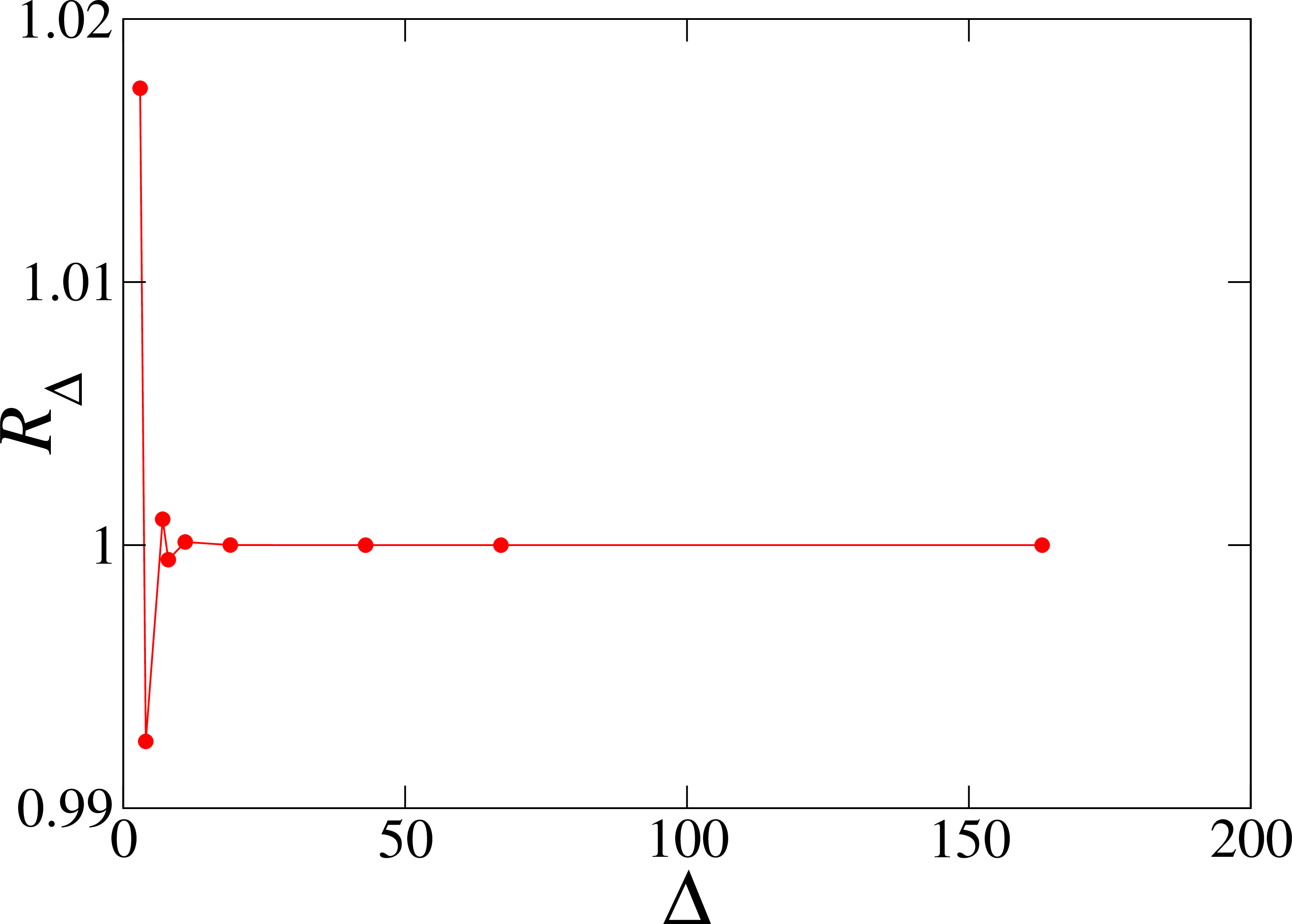
The above numerical values exhibit a fast decay as a function of the absolute discriminant \(\Delta\). This observation can be made quantitative by means of (86 ), yielding \[{\left\vert P_\Delta\right\vert}^2\approx4\pi^2{\left\vert q\right\vert}^{1/6}\approx4\pi^2\e^{-\pi\sqrt{\Delta}/6}\] when \(\Delta\) is large, up to tiny corrections proportional to \({\left\vert q\right\vert}=\e^{-\pi\sqrt{\Delta}}\). This is illustrated in figure 2, showing a plot of the ratio \[R_\Delta=\frac{\e^{\pi\sqrt{\Delta}/6}}{4\pi^2}\,{\left\vert P_\Delta\right\vert}^2 \label{rdef}\tag{89}\] against \(\Delta\), for all the nine imaginary quadratic fields.

It is a pleasure to thank Michel Bauer, Henri Cohen and Ricardo Pérez-Marco for useful exchanges.

References↩︎

References↩︎