Fully-heavy multiquarks in neural-network quantum states
June 23, 2026
Abstract
Exotic hadrons beyond the conventional quark model provide a direct window into the dynamics of strong interaction. However, extracting the multiquark spectroscopy has to face the quantum many-body problem, which is still a theoretical challenge. In this case, diquark-antidiquark model is proposed as an approximation. Although this model can describe the spectroscopy roughly, it cannot describe the detailed dynamics. Furthermore, the methods aiming at dealing with many-body problem, e.g. the Gaussian expansion method and Diffusion Monte Carlo, are proposed, but face severe computational bottlenecks. In this work, we introduce the neural-network quantum state (NNQS) approach to investigate the spectra of fully-heavy multiquark states within the non-relativistic potential quark model. By employing deep neural networks to represent the complex many-body spatial wave function, and constructing the color-spin part exactly from group theory to enforce fermionic antisymmetry, our approach effectively overcomes the dimensionality obstacles inherent in traditional methods. The results are compared with various model calculations, demonstrating that NNQS offers superior accuracy and flexibility, particularly in treating high-dimensional correlations. This work establishes NNQS as a promising tool for exploring the spectroscopy of exotic hadrons.
1 INTRODUCTION↩︎
Hadron spectroscopy is one of the most direct ways to shed light on the dynamics of the strong interaction. Due to color confinement in Quantum Chromodynamics (QCD), any color‑neutral object is allowed — not only the conventional mesons (\(q\bar{q}\)) and baryons (\(qqq\)) described by the quark model [1], [2]. Consequently, the search for exotic hadrons beyond the conventional quark model has become one of the most important frontiers in hadron physics. Since the first discovery of the \(X(3872)\) by the Belle Collaboration in 2003 [3], a large number of exotic hadron candidates have been observed experimentally, including the \(T^+_{cc}(3875)\) [4], [5], \(Z_c(3900)\) [6], [7], \(P_c\) [8]–[10], \(P_{cs}\) [11], and \(T_{cc\bar{c}\bar{c}}(6900)\) [12]. Several interpretations have been proposed to understand their internal structures [13]–[19], among which loosely bound hadronic molecules [13], [14] and compact multiquark states [14]–[16], [18], [20], [21] are the most intensively discussed. The former, having a larger size, corresponds to a bound state formed by the color‑neutral residual strong force, while the latter, with a smaller size, is a bound state formed directly by the fundamental color force.
Solving the quantum many-body problem for multiquark states presents significant theoretical challenges. For an \(N\)-quark system, the SU(3) color degree of freedom makes the system more complex than electron or nucleon systems. In previous studies, physical approximations such as the diquark-antidiquark model have been adopted to reduce the complexity of the system [14], [16], [18], [20]–[27]. Although this approximation can significantly reduce the system’s degrees of freedom, it artificially restricts the wave function to a specific configuration, ignoring the many-body correlation effects between (anti)quarks. Such configurations in wave function may lead to systematic errors and deviate from physical reality.
To overcome the above restricted configurations problem, more rigorous numerical methods are performed to directly solve multiquark systems. Currently, numerical approaches such as Diffusion Monte Carlo (DMC) [28], [29] and basis expansion methods, including the Gaussian expansion method (GEM) [30] and the explicitly correlated Gaussian (ECG) [31], [32] method, have been widely applied to solve multiquark systems. However, these methods face computational bottlenecks when dealing with multiquark systems. For basis expansion methods, the number of basis grows exponentially with the increasing number of quarks, making the precise solution of complex systems highly challenging. And the DMC method inevitably suffers from the fermion sign problem during imaginary time evolution, severely limiting its applicability to strongly correlated multiquark systems. Furthermore, wave function cusps [33] arising from the short-range color Coulomb interaction further increase the difficulty of convergence for traditional basis expansion methods.
Recently, machine learning techniques have provided a new approach to solving the quantum many-body problem. Motivated by their exceptional capacity to approximate high-dimensional functions [34], neural-network quantum states (NNQS) offer a flexible wave function representation capable of capturing complex many-body correlations efficiently [35]. This neural network based variational Monte Carlo (VMC) framework was implemented in quantum spin systems [36] and condensed matter physics [37], [38], as well as ab-initio chemistry problems [33], [39], [40]. Furthermore, this method has been effectively extended to nuclear physics [41]–[46]. Despite advancements across various subfields, the application of this method in hadron physics remained in the exploratory stage. Recently, the DeepQuark framework [47] was proposed, which marks the first successful implementation of the deep neural networks (DNNs) based VMC method in multiquark systems. These recent developments imply the feasibility of extending this method to multiquark systems.
In this work, we introduce NNQS approach to investigate the mass spectra of fully‑heavy multiquark states within the non‑relativistic potential quark model, with a particular focus on its advantages over the Gaussian expansion method (GEM). For the color-spin wave function, we construct it based on group theory and symmetry, ensuring that the trial wave function exactly satisfies the fermionic antisymmetry constraint. For the complex many-body spatial wave function, we entirely employ DNNs for high-dimensional fitting. This approach effectively overcomes the computational bottlenecks faced by traditional methods in solving high-dimensional spatial many-body correlations, thereby providing more accurate theoretical predictions for the mass spectra of fully-heavy multiquark systems. This paper is organized as follows. In Sec. 2, we introduce the nonrelativistic Hamiltonian of the system. The configurations of the multiquark states are constructed in Sec. 3. In Sec. 4, we detail the architecture of the neural-network wave function and the optimization procedure. Finally, the numerical results and discussions are presented in Sec. 5.
2 Hamiltonian↩︎
In this work, we adopt the nonrelativistic quark potential model (NRQPM) to describe fully-heavy multiquark states. The Hamiltonian is given by: \[H = \sum_{i}^{n}(m_i+ T_i ) + \sum_{i<j}^{n}V_{ij}(r_{ij}),\] where \(m_i\) and \(T_i\) denote the mass and kinetic energy of the \(i\)-th (anti)quark, respectively. The term \(V_{ij}(r_{ij})\) represents the effective potential between the \(i\)-th and \(j\)-th (anti)quarks, which depends on their relative distance \(r_{ij} = |\boldsymbol{r}_i - \boldsymbol{r}_j|\). The effective potential \(V_{ij}(r_{ij})\) consists of a one-gluon exchange (OGE) potential and a linear confinement potential [48], [49], written as \(V_{ij}(r_{ij}) = V_{ij}^{\text{OGE}}(r_{ij}) + V_{ij}^{\text{Conf}}(r_{ij})\). The form of \(V_{ij}^{\text{OGE}}\) and \(V_{ij}^{\text{Conf}}\) are given by, \[\begin{align} V_{ij}^{\text{OGE}} =& \frac{\alpha_{ij}}{4}(\boldsymbol{\lambda}_i \cdot \boldsymbol{\lambda}_j)\left [ \frac{1}{r_{ij}}-\frac{\pi}{2} \frac{\sigma_{ij}^{3}e^{-\sigma_{ij}^{2}r_{ij}^2}}{\pi^{3/2}}\frac{4}{3m_i m_j}(\boldsymbol{\sigma}_i\cdot\boldsymbol{\sigma}_j) \right ], \nonumber\\ V_{ij}^{\text{Conf}}=&-\frac{3}{16}(\boldsymbol{\lambda}_i \cdot \boldsymbol{\lambda}_j) br_{ij}, \label{eq:potential} \end{align}\tag{1}\] where \(\boldsymbol{\lambda}_i\) is the Gell-Mann matrix acting on the \(i\)-th quark (replaced by \(-\boldsymbol{\lambda}^{*}\) for antiquarks), and \(\boldsymbol{\sigma}_i\) represents the Pauli matrix. The parameters \(\alpha_{ij}\) and \(\sigma_{ij}\) are the strong coupling strength and the regulator of the spin-spin interaction, respectively. \(b\) is the strength of the linear confinement potential. The parameters of model are given in Table 1, which have been well determined by fitting the mass spectra of charmonium, bottomonium, and \(B_c\) mesons [48], [49].
| \(m_c/m_b\) (GeV) | 1.483/4.852 |
| \(\alpha_{cc}/\alpha_{bc}/\alpha_{bb}\) | 0.5461/0.5021/0.4311 |
| \(\sigma_{cc}/\sigma_{bc}/\sigma_{bb}\) (GeV) | 1.1384/1.3000/2.3200 |
| \(b\) (GeV\(^2\)) | 0.1425 |
7mm
3 The configuration of multiquarks↩︎
The total wave function of multiquark can be expressed as a direct product of the flavor, spatial, spin, and color wave functions: \[\Psi_{\text{total}} = \Psi_{\text{spatial}}\otimes \Psi_{\text{spin}}\otimes\Psi_{\text{color}}\otimes\Psi_{\text{flavor}}.\] In this work, the spin and color wave functions are constructed via \(\text{SU(3)} \otimes \text{SU(2)}\) symmetry, and the spatial wave function is parameterized by DNNs. Additionally, by considering only multiquark with identical flavors, the flavor wave function is symmetric.
For conventional mesons and baryons, the construction of their color-spin configurations is well established. For multiquark, the configurations become more complex. The absence of one-light-meson exchanges makes fully heavy systems highly favorable to form genuine compact multiquark configurations rather than conventional hadronic molecules [48], [49]. To describe such compact states, we adopt the \(\{Q_1Q_2\}\{\bar{Q}_3\bar{Q}_4\}\) configuration for fully-heavy tetraquarks 1, which includes the following systems: \(cc\bar{c}\bar{c}\), \(bb\bar{b}\bar{b}\), and \(bb\bar{c}\bar{c}\). In the color space, there exist two color-singlet bases for the tetraquark system, whose explicit forms are: \[\begin{align} \mathcal{C}_1= & \left|(Q_1Q_2)^6(\bar{Q}_3\bar{Q}_4)^{\bar{6}}\right\rangle,\\ \mathcal{C}_2= & \left|(Q_1Q_2)^{\bar{3}}(\bar{Q}_3\bar{Q}_4)^3\right\rangle. \label{eq:singlet} \end{align}\tag{2}\] Here, the superscripts denote the irreducible representations of the \(\text{SU(3)}\) color group for the diquark and antidiquark, respectively. Based on the \(\mathrm{SU}(3)\) Clebsch-Gordan(C-G) coefficients, the explicit forms of the color wave functions can be written as follows [48], [50]–[53]: \[\begin{align} \mathcal{C}_1= & \frac{1}{2\sqrt{6}} [ (rb + br)(\bar{b}\bar{r} + \bar{r}\bar{b}) + (gr + rg)(\bar{g}\bar{r} + \bar{r}\bar{g})\nonumber \\ & + (gb + bg)(\bar{b}\bar{g} + \bar{g}\bar{b}) + 2(rr)(\bar{r}\bar{r}) + 2(gg)(\bar{g}\bar{g}) \nonumber \\ & + 2(bb)(\bar{b}\bar{b}) ],\\ \mathcal{C}_2 = &\frac{1}{2\sqrt{3}} [ (br - rb)(\bar{b}\bar{r} - \bar{r}\bar{b}) - (rg - gr)(\bar{g}\bar{r} - \bar{r}\bar{g}) \nonumber\\ & + (bg - gb)(\bar{b}\bar{g} - \bar{g}\bar{b}) ]. \end{align}\] With the color wave functions, the matrix elements \(\langle \boldsymbol{\lambda}_i \cdot \boldsymbol{\lambda}_j \rangle\) can be evaluated [54], and the results are summarized in Table 2. It is worth mentioning that, according to the GEM in 2019 study [48], the contribution of the off-diagonal elements can be ignored. For simplicity, we only consider the diagonal matrix elements results in this work to compare the two methods.
| \(\hat{O}\) | \(\bm{\lambda}_1 \cdot\bm{\lambda}_2\) | \(\bm{\lambda}_1 \cdot\bm{\lambda}_3\) | \(\bm{\lambda}_1 \cdot\bm{\lambda}_4\) | \(\bm{\lambda}_2 \cdot\bm{\lambda}_3\) | \(\bm{\lambda}_2 \cdot\bm{\lambda}_4\) | \(\bm{\lambda}_3 \cdot\bm{\lambda}_4\) |
|---|---|---|---|---|---|---|
| \(\langle\mathcal{C}_1| \hat{O}| \mathcal{C}_1 \rangle\) | 4/3 | -10/3 | -10/3 | -10/3 | -10/3 | 4/3 |
| \(\langle\mathcal{C}_2| \hat{O}| \mathcal{C}_2 \rangle\) | -8/3 | -4/3 | -4/3 | -4/3 | -4/3 | -8/3 |
0.1mm
In the spin space, the total spin of the system can take values of \(J=0\), \(1\), and \(2\), are represented as follows: \[\begin{align} \mathcal{S}_1 &= |(Q_1 Q_2)_0 (\bar{Q}_3 \bar{Q}_4)_0 \rangle_0, \\[2ex] \mathcal{S}_2 &= |(Q_1 Q_2)_1 (\bar{Q}_3 \bar{Q}_4)_1 \rangle_0, \\[2ex] \mathcal{S}_3 &= |(Q_1 Q_2)_0 (\bar{Q}_3 \bar{Q}_4)_1 \rangle_1, \\[2ex] \mathcal{S}_4 &= |(Q_1 Q_2)_1 (\bar{Q}_3 \bar{Q}_4)_0 \rangle_1, \\[2ex] \mathcal{S}_5 &= |(Q_1 Q_2)_1 (\bar{Q}_3 \bar{Q}_4)_1 \rangle_1, \\[2ex] \mathcal{S}_6 &= |(Q_1 Q_2)_1 (\bar{Q}_3 \bar{Q}_4)_1 \rangle_2. \end{align}\] Here, the subscript denotes spin quantum number. Based on the \(\mathrm{SU}(2)\) C-G coefficients, the explicit forms of the spin wave functions can be written as follows [48]: \[\begin{align} \mathcal{S}_1 &= \frac{1}{2} (\uparrow\downarrow\uparrow\downarrow - \uparrow\downarrow\downarrow\uparrow - \downarrow\uparrow\uparrow\downarrow + \downarrow\uparrow\downarrow\uparrow), \\[1ex] \mathcal{S}_2 &= \sqrt{\frac{1}{12}} (2\uparrow\uparrow\downarrow\downarrow - \uparrow\downarrow\uparrow\downarrow - \uparrow\downarrow\downarrow\uparrow \notag \\ &\quad - \downarrow\uparrow\uparrow\downarrow - \downarrow\uparrow\downarrow\uparrow + 2\downarrow\downarrow\uparrow\uparrow), \\[1ex] \mathcal{S}_3 &= \sqrt{\frac{1}{2}} (\uparrow\downarrow\uparrow\uparrow - \downarrow\uparrow\uparrow\uparrow), \\[1ex] \mathcal{S}_4 &= \sqrt{\frac{1}{2}} (\uparrow\uparrow\uparrow\downarrow - \uparrow\uparrow\downarrow\uparrow), \\[1ex] \mathcal{S}_5 &= \frac{1}{2} (\uparrow\uparrow\uparrow\downarrow + \uparrow\uparrow\downarrow\uparrow - \uparrow\downarrow\uparrow\uparrow - \downarrow\uparrow\uparrow\uparrow), \\[1ex] \mathcal{S}_6 &= \uparrow\uparrow\uparrow\uparrow. \end{align}\] With the spin wave functions, the matrix elements \(\left \langle\boldsymbol{\sigma}_i\cdot\boldsymbol{\sigma}_j\right \rangle\) can be evaluated [54], and the results are summarized in Table 3.
| \(\hat{O}\) | \(\bm{\sigma}_1 \cdot\bm{\sigma}_2\) | \(\bm{\sigma}_1 \cdot\bm{\sigma}_3\) | \(\bm{\sigma}_1 \cdot\bm{\sigma}_4\) | \(\bm{\sigma}_2 \cdot\bm{\sigma}_3\) | \(\bm{\sigma}_2 \cdot\bm{\sigma}_4\) | \(\bm{\sigma}_3 \cdot\bm{\sigma}_4\) |
|---|---|---|---|---|---|---|
| \(\langle\mathcal{S}_1|\hat{O}|\mathcal{S}_1\rangle\) | -3 | 0 | 0 | 0 | 0 | -3 |
| \(\langle\mathcal{S}_2|\hat{O}|\mathcal{S}_2\rangle\) | 1 | -2 | -2 | -2 | -2 | 1 |
| \(\langle\mathcal{S}_3|\hat{O}|\mathcal{S}_3\rangle\) | -3 | 0 | 0 | 0 | 0 | 1 |
| \(\langle\mathcal{S}_4|\hat{O}|\mathcal{S}_4\rangle\) | 1 | 0 | 0 | 0 | 0 | -3 |
| \(\langle\mathcal{S}_5|\hat{O}|\mathcal{S}_5\rangle\) | 1 | -1 | -1 | -1 | -1 | 1 |
| \(\langle\mathcal{S}_6|\hat{O}|\mathcal{S}_6\rangle\) | 1 | 1 | 1 | 1 | 1 | 1 |
0mm
For simplicity, we consider the \(\{Q_1Q_2Q_3Q_4\}\bar{Q}_5\) configuration for fully-heavy pentaquarks, where the four quarks are identical flavors, which includes the following systems: \(cccc\bar{c}\), \(cccc\bar{b}\), \(bbbb\bar{b}\), and \(bbbb\bar{c}\). In the color space, three color-singlet states can be constructed via the SU(3) group theory. Its Young tableau representation is given by [55]: \[C_1 = {\begin{array}{|c|c|} \hline 1 & 4 \\ \hline 2 & \multicolumn{1}{c}{} \\ \cline{1-1} 3 & \multicolumn{1}{c}{} \\ \cline{1-1} \end{array}}_{\;3} \otimes (5)_{\bar{3}},~ C_2 = {\begin{array}{|c|c|} \hline 1 & 2 \\ \hline 3 & \multicolumn{1}{c}{} \\ \cline{1-1} 4 & \multicolumn{1}{c}{} \\ \cline{1-1} \end{array}}_{\;3} \otimes (5)_{\bar{3}},~ C_3 = {\begin{array}{|c|c|} \hline 1 & 3 \\ \hline 2 & \multicolumn{1}{c}{} \\ \cline{1-1} 4 & \multicolumn{1}{c}{} \\ \cline{1-1} \end{array}}_{\;3} \otimes (5)_{\bar{3}}.\] Using the \(\mathrm{SU}(3)\) C-G coefficients [53], the explicit forms of the color wave functions for the pentaquark can be written as follows [56]: \[\begin{align} C_1 &= \frac{1}{3\sqrt{2}} (grbb - rgbb + rbgb - brgb + bgrb - gbrb)\bar{b}\nonumber \\ &\quad + (grbr - rgbr + rbgr - brgr + bgrr - gbrr)\bar{r} \nonumber\\ &\quad + (grbg - rgbg + rbgg - brgg + bgrg - gbrg)\bar{g},\\ C_2 &= \frac{1}{4\sqrt{3}} (2bbgr - 2bbrg + gbrb - gbbr + bgrb - bgbr \nonumber\\ &\quad - rbgb + rbbg - brgb + brbg)\bar{b} + (2rrbg - 2rrgb \nonumber\\ &\quad + rgrb - rgbr + grrb - grbr + rbgr - rbrg + brgr \nonumber\\ &\quad - brrg)\bar{r} + (2ggrb - 2ggbr - rggb + rgbg - grgb \nonumber\\ &\quad + grbg + gbgr - gbrg + bggr - bgrg)\bar{g}],\\ C_3 &= \frac{1}{12} (3bgbr - 3gbbr - 3brbg + 3rbbg - rbgb - 2rgbb \nonumber\\ &\quad + 2grbb + brgb + gbrb - bgrb)\bar{b} + (3grrb - 3rgrb\nonumber \\ &\quad - 3brrg + 3rbrg - rbgr - 2gbrr + 2bgrr - grbr\nonumber \\ &\quad + rgbr + brgr)\bar{r} + (3grgb - 3rggb + 3bggr - 3gbgr \nonumber\\ &\quad - grbg + rgbg + 2rbgg - 2brgg + gbrg - bgrg)\bar{g}. \end{align}\]
In the spin space, based on the \(\text{SU(2)}\) coupling rules, the total spin of the system can take values of \(J=5/2, 3/2\), and \(1/2\), and their corresponding Young tableaux are represented as follows: \[\begin{align} \ytableausetup{boxsize=1.2em} J = \frac{5}{2}: \quad & S_1 = \begin{ytableau} 1 & 2 & 3 & 4 & 5 \end{ytableau} . \\[3ex] J = \frac{3}{2}: \quad & S_2 = \begin{ytableau} 1 & 2 & 3 & 4 \\ 5 \end{ytableau} , \, S_3 = \begin{ytableau} 1 & 2 & 3 & 5 \\ 4 \end{ytableau} , \notag \\ & S_4 = \begin{ytableau} 1 & 3 & 4 & 5 \\ 2 \end{ytableau} , \, S_5 = \begin{ytableau} 1 & 2 & 4 & 5 \\ 3 \end{ytableau} . \\[3ex] J = \frac{1}{2}: \quad & S_6 = \begin{ytableau} 1 & 2 & 3 \\ 4 & 5 \end{ytableau} , \, S_7 = \begin{ytableau} 1 & 3 & 4 \\ 2 & 5 \end{ytableau} , \, S_8 = \begin{ytableau} 1 & 2 & 4 \\ 3 & 5 \end{ytableau} , \notag \\ & S_9 = \begin{ytableau} 1 & 2 & 5 \\ 3 & 4 \end{ytableau} , \, S_{10} = \begin{ytableau} 1 & 3 & 5 \\ 2 & 4 \end{ytableau} . \end{align}\] Incorporating the \(\mathrm{SU}(2)\) C-G coefficients, the explicit forms of the pentaquark spin wave functions can be derived: \[\begin{align} S_1 =&\uparrow \uparrow \uparrow \uparrow \uparrow, \\ S_2 =&\frac{1}{2\sqrt{5}}(4\uparrow \uparrow \uparrow \uparrow \downarrow -\uparrow \uparrow \uparrow \downarrow \uparrow -\uparrow \uparrow \downarrow \uparrow \uparrow -\uparrow \downarrow \uparrow \uparrow \uparrow -\downarrow \uparrow \uparrow \uparrow \uparrow),\\ S_3 =& \frac{1}{2\sqrt{3}} (3\uparrow\uparrow\uparrow\downarrow - \uparrow\uparrow\downarrow\uparrow - \uparrow\downarrow\uparrow\uparrow - \downarrow\uparrow\uparrow\uparrow), \\ S_4 =& \frac{1}{\sqrt{2}} (\uparrow\downarrow\uparrow\uparrow\uparrow - \downarrow\uparrow\uparrow\uparrow\uparrow), \\ S_5 =& \frac{1}{\sqrt{6}} (2\uparrow\uparrow\downarrow\uparrow\uparrow - \uparrow\downarrow\uparrow\uparrow\uparrow - \downarrow\uparrow\uparrow\uparrow\uparrow), \end{align}\] \[\begin{align} S_6 =& \frac{1}{3\sqrt{2}} \Bigl( 3\uparrow\uparrow\uparrow\downarrow\downarrow - \uparrow\uparrow\downarrow\uparrow\downarrow - \uparrow\downarrow\uparrow\uparrow\downarrow - \downarrow\uparrow\uparrow\uparrow\downarrow - \uparrow\uparrow\downarrow\downarrow\uparrow \nonumber \\ & - \uparrow\downarrow\uparrow\downarrow\uparrow - \downarrow\uparrow\uparrow\downarrow\uparrow + \uparrow\downarrow\downarrow\uparrow\uparrow + \downarrow\uparrow\downarrow\uparrow\uparrow + \downarrow\downarrow\uparrow\uparrow\uparrow \Bigr), \\ S_7 =& \frac{1}{2\sqrt{3}} (2\uparrow\downarrow\uparrow\uparrow\downarrow - 2\downarrow\uparrow\uparrow\uparrow\downarrow - \uparrow\downarrow\downarrow\uparrow\uparrow+ \downarrow\uparrow\downarrow\uparrow\uparrow - \uparrow\downarrow\uparrow\downarrow\uparrow\nonumber \\ & + \downarrow\uparrow\uparrow\downarrow\uparrow), \\ S_8 =& \frac{1}{6} \Bigl( 4\uparrow\uparrow\downarrow\uparrow\downarrow - 2\uparrow\downarrow\uparrow\uparrow\downarrow - 2\downarrow\uparrow\uparrow\uparrow\downarrow - 2\uparrow\uparrow\downarrow\downarrow\uparrow+ 2\downarrow\downarrow\uparrow\uparrow\uparrow \nonumber \\ & + \uparrow\downarrow\uparrow\downarrow\uparrow + \downarrow\uparrow\uparrow\downarrow\uparrow - \uparrow\downarrow\downarrow\uparrow\uparrow - \downarrow\uparrow\downarrow\uparrow\uparrow \Bigr), \\ S_9 =& \frac{1}{2\sqrt{3}} (2\uparrow\uparrow\downarrow\downarrow\uparrow + 2\downarrow\downarrow\uparrow\uparrow\uparrow - \uparrow\downarrow\uparrow\downarrow\uparrow- \downarrow\uparrow\uparrow\downarrow\uparrow - \uparrow\downarrow\downarrow\uparrow\uparrow\nonumber\\ & - \downarrow\uparrow\downarrow\uparrow\uparrow),\\ S_{10} =&\frac{1}{2}(\uparrow \downarrow \uparrow \downarrow \uparrow -\uparrow \downarrow \downarrow \uparrow \uparrow -\downarrow \uparrow \uparrow \downarrow \uparrow +\downarrow \uparrow \downarrow \uparrow \uparrow ). \end{align}\]
By combining the color and spin wave functions with the C-G coefficients of the \(S_4\) permutation group [57], the color-spin wave functions \(\Psi^{\text{CS}}\) can be constructed as follows. For the \(S\)-wave pentaquark system with the \(\{Q_1Q_2Q_3Q_4\}\bar{Q}_5\) configuration, there are two wave functions corresponding to \(J^P = 3/2^-\) and \(1/2^-\): \[\begin{align} \Psi^{\text{CS}}_{3/2^-} &= \frac{1}{\sqrt{3}} (C_1 S_3 + C_2 S_4 - C_3 S_5), \\[1ex] \Psi^{\text{CS}}_{1/2^-} &= \frac{1}{\sqrt{3}} (C_1 S_6 + C_2 S_7 - C_3 S_8). \label{eq:CSwavefunction} \end{align}\tag{3}\] One notices that there is no \(J^P=5/2^-\) pentaquark in this configuration, as it violates Fermi-Dirac statistics. It is worth mentioning that since both the spatial and flavor wave functions of the \(\{Q_1Q_2Q_3Q_4\}\) identical quarks are symmetric, the Pauli principle dictates that their color-spin wave function must be totally antisymmetric. States with a total spin of \(J^P=5/2^-\) are forbidden for such pentaquark configurations.
| \((i,j)\) | \(\left\langle\bm\lambda_i\cdot \bm\lambda_j \right \rangle\) | \(\left\langle(\bm\lambda_i\cdot \bm\lambda_j)(\bm\sigma_i\cdot \bm\sigma_j) \right \rangle_{\frac{3}{2}^{-}}\) | \(\left\langle(\bm\lambda_i\cdot \bm\lambda_j)(\bm\sigma_i\cdot \bm\sigma_j)\right \rangle_{\frac{1}{2}^{-}}\) |
|---|---|---|---|
| \((1,2)\) | -4/3 | -28/9 | -28/9 |
| \((1,3)\) | -4/3 | -28/9 | -28/9 |
| \((1,4)\) | -4/3 | -28/9 | -28/9 |
| \((1,5)\) | -4/3 | 4/3 | -8/3 |
| \((2,3)\) | -4/3 | -28/9 | -28/9 |
| \((2,4)\) | -4/3 | -28/9 | -28/9 |
| \((2,5)\) | -4/3 | 4/3 | -8/3 |
| \((3,4)\) | -4/3 | -28/9 | -28/9 |
| \((3,5)\) | -4/3 | 4/3 | -8/3 |
| \((4,5)\) | -4/3 | 4/3 | -8/3 |
1mm
Based on the color-spin wave functions, one can evaluate the interactions within pentaquarks. Because the potential of \(V^{\text{Conf}}\) term depends on color interactions, it yields only diagonal matrix elements due to the orthogonality of the wave functions. The term \(V^{\text{OGE}}\) contains color-spin interactions, both diagonal and off-diagonal elements are evaluated. The calculated results are summarized in Table 4, where the subscript of the color-spin interactions, \(\left\langle\cdots\right \rangle_{\frac{3}{2}^{-}}\) and \(\left\langle\cdots\right \rangle_{\frac{1}{2}^{-}}\), indicate that the operator acts on different color-spin wave functions.
4 Neural-network wave function↩︎
For the spatial wave function of multiquarks, it was determined by solving the many-body Schrödinger equation. Exactly solving the Schrödinger equation for multiquarks is a high-dimensional quantum many-body problem. To investigate the ground state properties of the system, we employ the variational method, the parameters of the trial wave function \(\Psi_{\theta}\) are optimized by minimizing the value of energy expectation. \[E_{\theta}=\frac{\left \langle \Psi_{\theta } \right |H\left | \Psi_{\theta } \right \rangle }{\left \langle \Psi_{\theta } | \Psi_{\theta } \right \rangle }\ge E_0.\] We employ DNNs to parameterize \(\Psi_{\text{spatial}}\). We introduce the three-dimensional coordinates of all quarks \(\boldsymbol{r}_1, \boldsymbol{r}_2, \dots, \boldsymbol{r}_n\), which constitute a \(3n\)-dimensional vector. To remove the kinetic energy contribution from the center of mass motion [58], we define the internal coordinates \(\bar{\boldsymbol{r}}_1, \bar{\boldsymbol{r}}_2, \dots, \bar{\boldsymbol{r}}_n\) as the neural network input, where \(\bar{\boldsymbol{r}_i}=\boldsymbol{r}_i-\boldsymbol{R}_{\text{CM}}\), \(\boldsymbol{R}_{\text{CM}}\) is the center of mass coordinate of the system. The scalar output of the network is \(\ln(\Psi_{\text{spatial}})\). This logarithmic representation is adopted to prevent numerical instabilities during the Monte Carlo sampling. To ensure the symmetry of the spatial wave function, we symmetrize the neural network wave function. Furthermore, we added a Gaussian function \(-\alpha \sum_{i=1}^n |\bar{\boldsymbol{r}}_i|^2\) to confine the particle within a finite volume [41], where the parameter \(\alpha = 0.05\).
We employ a fully connected neural network for this work. Each hidden layer applies a linear function to its inputs, followed by a nonlinear activation function: \[\bar{\boldsymbol{r}}^{(l+1)} = f(\boldsymbol{\omega}^{(l)}\bar{\boldsymbol{r}}^{(l)}+b^{(l)}),\] where \(\boldsymbol{\omega}^{(l)}\) and \(b^{(l)}\) denote the weights and biases of the \(l\)-th layer, respectively, and \(f\) is the activation function. We employ the Sigmoid Linear Unit (SiLU) as the activation function in this work. Its specific form is expressed as: \[\text{SiLU}(x) = \frac{x}{1 + e^{-x}}.\] For meson and baryon systems, the network consists of 4 hidden layers with 24 nodes per layer. For tetraquark and pentaquark systems, the network has 6 hidden layers with 32 nodes each. This design ensures sufficient expressive power while preserving computational feasibility.
To obtain the optimal parameters \(\theta\) that minimize the energy expectation value \(E_{\theta}\), We employ the stochastic reconfiguration (SR) algorithm to optimize the variational parameters [59], [60]. The SR algorithm is equivalent to performing imaginary-time evolution in the variational manifold and is closely related to the natural gradient descent method in unsupervised learning [41], [61]. Compared to standard gradient descent, the SR approach enhances optimization stability. Specifically, at each iteration, we use Metropolis-Hastings Monte Carlo sampling [62], [63] generates a large coordinate samples, which distributed as \(|\Psi_{\theta}|^2\). During the sampling process, a cutoff is introduced to resolve the issue of potential singularities in Eq. 1 . From these samples, the energy expectation \(E_{\theta}\) and its gradients \(\nabla_{\theta}E_{\theta}\) are evaluated. The \(\nabla_{\theta}E_{\theta}\) is calculated using the following formula: \[\nabla_{\theta}E_{\theta}=2\left(\frac{\left\langle\partial {\psi_{\theta }}\right|H\left | \psi_{\theta } \right \rangle }{\left \langle \psi_{\theta } | \psi_{\theta } \right \rangle }-E_{\theta}\frac{\left \langle \partial \psi_{\theta } | \psi_{\theta } \right \rangle }{\left \langle \psi_{\theta } | \psi_{\theta } \right \rangle }\right ),\] where \(|\partial \psi_\theta\rangle \equiv \partial |\psi_\theta\rangle / \partial \theta\), \(S\) matrix denotes the quantum fisher information matrix, which is defined as: \[S_{ab} = \frac{\langle \partial_a \psi_\theta | \partial_b \psi_\theta \rangle}{\langle \psi_\theta | \psi_\theta \rangle} - \frac{\langle \partial_a \psi_\theta | \psi_\theta \rangle \langle \psi_\theta | \partial_b \psi_\theta \rangle}{\langle \psi_\theta | \psi_\theta \rangle^2}.\]
By calculating \(\nabla_{\theta}E\) and the \(S\) matrix, the parameters of the neural network can be updated through the parameter update rule, which is given by: \[\begin{align} \theta^{i+1}=\theta^i-\eta(S+\epsilon I)^{-1}\nabla_{\theta^i}E_{\theta^i}, \end{align}\] where \(i\) is the iteration step, \(\eta\) is the learning rate, \(\epsilon\) is a small regularization constant set between \(10^{-3}\) and \(10^{-4}\) introduced to ensure matrix invertibility and \(I\) is the identity matrix. After hundreds of iterations, the energy expectation value converges to a minimum, yielding a neural-network wave function that approximates the ground state.
To accelerate the optimization process, we use a small batch size during the early stage. As optimization enters the final 30 steps, we increase the batch size from 2000 to 80,000 to reduce statistical errors. Throughout iterations, the learning rate decayed from \(10^{-1}\) to \(10^{-5}\). To describe the random error of the SR algorithm, we employ a multi-step averaging scheme in the final stage of optimization. Specifically, we take the average of the masses from the final 10 iterations as our final result. Consequently, the total error \(\delta_{\text{tot}}\) is obtained by combining the Monte Carlo statistical error \(\delta_{\text{MC}}\) and the neural network error \(\delta_{\text{NN}}\), the \(\delta_{\text{tot}}\) is given by: \[\delta_{\text{tot}} = \sqrt{\delta_{\text{MC}}^2 + \delta_{\text{NN}}^2},\] where \(\delta_{\text{NN}}\) is the standard deviation of the last ten iterations. All of the above calculations were carried out within the PyTorch [64] framework.
5 Results and discussion↩︎
In this section, we present the mass spectra of fully-heavy multiquark systems calculated via NNQS. All numerical calculations in this work focus exclusively on the \(S\)-wave ground states. Before applying the NNQS method to fully-heavy multiquark, we first tested it on conventional mesons and baryons. The results are summarized in TABLE 5.
| State | \(J^P\) | This work | GEM | Exp. |
|---|---|---|---|---|
| \(\eta_c\) | \(0^-\) | \(2983.7(10)\) | 2983 | 2984 |
| \(J/\psi\) | \(1^-\) | \(3097.2(8)\) | 3097 | 3097 |
| \(B_c\) | \(0^-\) | \(6270.7(9)\) | 6271 | 6274 |
| \(B_{c}^{\ast}\) | \(1^-\) | \(6326.3(10)\) | 6328 | \(\cdots\) |
| \(\eta_b\) | \(0^-\) | \(9389.4(18)\) | 9390 | 9399 |
| \(\Upsilon\) | \(1^-\) | \(9460.0(12)\) | 9460 | 9460 |
| \(\Omega_{ccc}\) | \(3/2^+\) | \(4816.1(5)\) | 4823 | \(\cdots\) |
| \(\Omega_{bbb}\) | \(3/2^+\) | \(14408.0(9)\) | 14421 | \(\cdots\) |
| \(\Omega_{ccb}\) | \(1/2^+\) | \(8025.3(7)\) | 8034 | \(\cdots\) |
| \(\Omega_{ccb}^{\ast}\) | \(3/2^+\) | \(8050.3(6)\) | 8057 | \(\cdots\) |
| \(\Omega_{cbb}\) | \(1/2^+\) | \(11217.6(8)\) | 11222 | \(\cdots\) |
| \(\Omega_{cbb}^{\ast}\) | \(3/2^+\) | \(11246.1(7)\) | 11250 | \(\cdots\) |
4mm
![Figure 1: The mass estimate as a function of iteration steps for cc\bar{c}\bar{c} tetraquark configurations (a)\left|\left \{ cc \right \}_0^6\left \{ \bar{c}\bar{c} \right \}_0^{\bar{6}}\right \rangle _0^0, (b)\left |\left \{ cc \right \}_1^{\bar{3}}\left \{ \bar{c}\bar{c} \right \}_1^3 \right \rangle _0^0, (c)\left |\left \{ cc \right \}_1^{\bar{3}}\left \{ \bar{c}\bar{c} \right \}_1^3 \right \rangle _1^0 and (d)\left |\left \{ cc \right \}_1^{\bar{3}}\left \{ \bar{c}\bar{c} \right \}_1^3 \right \rangle _2^0 in the optimization progress. The Monte Carlo statistical errors of the masses are shown by the blue shaded area, and red dashed line represents the GEM results [48]. The insets in each subplot magnifies the final optimization stage.](/article/2606.24380/fig/NNtetraquark.png "fig:")
For meson, the results show that the masses using our method agree with those from the GEM as shown in Table 5. This shows that the neural-network wave function is capable of effectively describing the spatial correlations of the two-body system. When the number of (anti)quarks increase to three, i.e. baryons, the superiority of the NNQS method becomes prominent. The masses of baryons in this work are lower about 4 to 13 MeV than those in Ref. [49], implying that our variational method produces results very close to the exact values. This suggests that the neural-network wave function has stronger expressive power than trial wave function constructed with GEM. The reason is that the spatial wave function of many-body systems is complex. The neural network, as a universal function approximator without the need for predefined functional forms, can capture the internal spatial distribution of three-body and more complex systems.
And then, we extend our method to fully-heavy tetraquark. The optimization performance of NNQS in tetraquark is shown in Figure 1, and we take different quantum number \(cc\bar{c}\bar{c}\) systems as examples. The mass expectation for the four configurations decrease rapidly during the initial optimization phase, converging stably below the GEM results [48]. The Monte Carlo statistical uncertainties (blue shaded in Fig. 1) limited and stable, confirming that the NNQS method provides a reliable prediction.
| State | \(J^{P}\) | Configuration | Mass |
|---|---|---|---|
| \(cc\bar{c}\bar{c}\) | \(0^{+}_{6\bar{6}}\) | \(\left |\left \{ cc \right \}_0^6\left \{ \bar{c}\bar{c} \right \}_0^{\bar{6}} \right \rangle _0^0\) | \(6416.4(8)\) |
| \(0^{+}_{\bar{3}3}\) | \(\left |\left \{ cc \right \}_1^{\bar{3}}\left \{ \bar{c}\bar{c} \right \}_1^3 \right \rangle _0^0\) | \(6466.2(7)\) | |
| \(1^{+}\) | \(\left |\left \{ cc \right \}_1^{\bar{3}}\left \{ \bar{c}\bar{c} \right \}_1^3 \right \rangle _1^0\) | \(6479.0(7)\) | |
| \(2^{+}\) | \(\left |\left \{ cc \right \}_1^{\bar{3}}\left \{ \bar{c}\bar{c} \right \}_1^3 \right \rangle _2^0\) | \(6503.8(8)\) | |
| \(bb\bar{b}\bar{b}\) | \(0^{+}_{6\bar{6}}\) | \(\left |\left \{ bb \right \}_0^6\left \{ \bar{b}\bar{b} \right \}_0^{\bar{6}} \right \rangle _0^0\) | \(19209.1(11)\) |
| \(0^{+}_{\bar{3}3}\) | \(\left |\left \{ bb \right \}_1^{\bar{3}}\left \{ \bar{b}\bar{b} \right \}_1^3 \right \rangle _0^0\) | \(19286.4(11)\) | |
| \(1^{+}\) | \(\left |\left \{ bb \right \}_1^{\bar{3}}\left \{ \bar{b}\bar{b} \right \}_1^3 \right \rangle _1^0\) | \(19294.2(12)\) | |
| \(2^{+}\) | \(\left |\left \{ bb \right \}_1^{\bar{3}}\left \{ \bar{b}\bar{b} \right \}_1^3 \right \rangle _2^0\) | \(19306.9(10)\) | |
| \(bb\bar{c}\bar{c}\) | \(0^{+}_{6\bar{6}}\) | \(\left |\left \{ bb \right \}_0^6\left \{ \bar{c}\bar{c} \right \}_0^{\bar{6}} \right \rangle _0^0\) | \(12872.7(8)\) |
| \(0^{+}_{\bar{3}3}\) | \(\left |\left \{ bb \right \}_1^{\bar{3}}\left \{ \bar{c}\bar{c} \right \}_1^3 \right \rangle _0^0\) | \(12919.6(7)\) | |
| \(1^{+}\) | \(\left |\left \{ bb \right \}_1^{\bar{3}}\left \{ \bar{c}\bar{c} \right \}_1^3 \right \rangle _1^0\) | \(12926.2(9)\) | |
| \(2^{+}\) | \(\left |\left \{ bb \right \}_1^{\bar{3}}\left \{ \bar{c}\bar{c} \right \}_1^3 \right \rangle _2^0\) | \(12939.6(8)\) |
4mm
All predicted mass spectra for the \(cc\bar{c}\bar{c}\), \(bb\bar{b}\bar{b}\), and \(bb\bar{c}\bar{c}\) systems has been collected in Table 6. We label the two configurations of the \(J^P=0^+\) state \(\left |\left \{ QQ \right \}_0^6\left \{ \bar{Q}\bar{Q} \right \}_0^{\bar{6}} \right \rangle _0^0\) and \(\left |\left \{ QQ \right \}_1^{\bar{3}}\left \{ \bar{Q}\bar{Q} \right \}_1^3 \right \rangle _0^0\) as \(0^{+}_{6\bar{6}}\) and \(0^{+}_{\bar{3}3}\), respectively. It is found that the mass of the \(0^{+}_{\bar{3}3}\) state is slightly larger than that of \(0^{+}_{6\bar{6}}\) state. In all tetraquark systems, the mass splitting between these two \(J^P=0^+\) states is about 40 to 80 MeV. The other two \(J^P=1^+\) and \(J^P=2^+\) fully charm tetraquarks are \(6479.0\pm 0.7~\mathrm{MeV}\) and \(6503.8\pm 0.8~\mathrm{MeV}\), respectively, significantly lower than the values from GEM [48]. The mass splitting between these two states is about 25 MeV. These masses and the mass splitting indicate that the observed \(X(6900)\) cannot be an \(S\)-wave ground fully charmed tetraquark state.
![Figure 2: A comparison of the predicted masses of the tetraquark states cc\bar{c}\bar{c} (a), bb\bar{b}\bar{b} (b), and bb\bar{c}\bar{c} (c). The blue points, red triangles, and green squares represent this work predictions, the GEM predictions in 2019 [48], and 2026 [66], respectively. The GEM results in 2026 are the unmixed 0^{+}_{6\bar{6}} and 0^{+}_{\bar{3}3} configurations.](/article/2606.24380/fig/tetraquark_comparison_with_GEM.png "fig:")
| \(J^P\) | \(0^{+}_{6\bar{6}}\) | \(0^{+}_{\bar{3}3}\) | \(1^{+}\) | \(2^{+}\) |
|---|---|---|---|---|
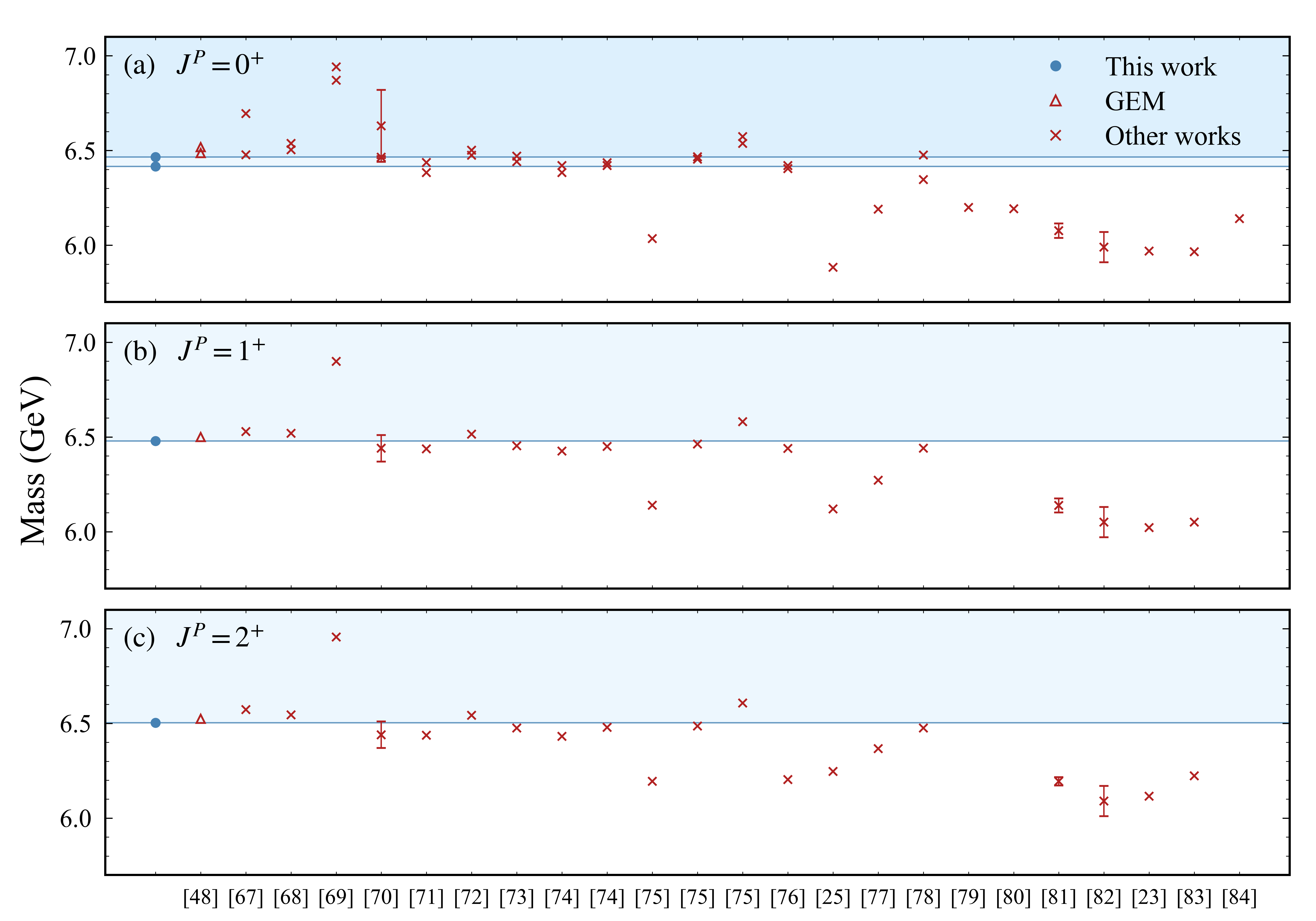
| This work | \(6416.4(8)\) | \(6466.2(17)\) | \(6479.0(7)\) | \(6503.8(8)\) |
| Ref. [48] | 6518 | 6487 | 6500 | 6524 |
| Ref. [67] | 6695 | 6477 | 6528 | 6573 |
| Ref. [68] | 6537 | 6504 | 6519 | 6545 |
| Ref. [69] | 6942 | 6871 | 6899 | 6956 |
| Ref. [70] | 6440-6820 | 6460-6470 | 6370-6510 | 6370-6510 |
| Ref. [71] | 6383 | 6437 | 6437 | 6437 |
| Ref. [72] | 6475 | 6501 | 6515 | 6543 |
| Ref. [73] | 6470 | 6441 | 6453 | 6475 |
| Ref. [74] | 6383 | 6420 | 6425 | 6432 |
| Ref. [74] | 6421 | 6436 | 6450 | 6479 |
| Ref. [75] | \(\cdots\) | 6035 | 6139 | 6194 |
| Ref. [75] | 6467 | 6454 | 6463 | 6486 |
| Ref. [75] | 6537 | 6573 | 6580 | 6607 |
| Ref. [76] | 6404 | 6421 | 6439 | 6204 |
| Ref. [25] | \(\cdots\) | 5883 | 6120 | 6246 |
| Ref. [77] | \(\cdots\) | 6190 | 6271 | 6367 |
| Ref. [78] | 6476 | 6346 | 6441 | 6475 |
| Ref. [79] | \(\cdots\) | 6200 | \(\cdots\) | \(\cdots\) |
| Ref. [80] | \(\cdots\) | 6192 | \(\cdots\) | \(\cdots\) |
| Ref. [81] | \(\cdots\) | 6038-6115 | 6101-6176 | 6172-6216 |
| Ref. [82] | \(\cdots\) | 5990(80) | 6050(80) | 6090(80) |
| Ref. [23] | \(\cdots\) | 5969 | 6021 | 6115 |
| Ref. [83] | \(\cdots\) | 5966 | 6051 | 6223 |
| Ref. [84] | \(\cdots\) | \(<\)6140 | \(\cdots\) | \(\cdots\) |
1mm
In Figure 2, we present the mass spectra of these tetraquark states and compare them with the results from GEM. For the \(cc\bar{c}\bar{c}\) system, in Figure 2 (a), the masses of states \(J^P=0^{+}_{\bar{3}3}\), \(J^P=1^+\) and \(J^P=2^+\) are lower than the GEM [48] predictions by approximately 20 MeV, the mass of state \(J^P=0^{+}_{6\bar{6}}\) is lower than the GEM predictions by approximately 101 MeV. For the \(bb\bar{b}\bar{b}\) system in Figure 2 (b), the masses of states \(J^P=0^{+}_{\bar{3}3}\), \(J^P=1^+\) and \(J^P=2^+\) are lower than the GEM predictions by approximately 35 MeV, the mass of state \(J^P=0^{+}_{6\bar{6}}\) is lower than the GEM predictions by approximately 128 MeV. The above results show that for tetraquarks, the mass expectations from the NNQS are obviously lower than GEM predictions. This shows that neural-network wave function has a stronger expressive power for the multiquark wave function than GEM, as indicated by the variational principle. This discrepancy originates from the difference in the expressive power of the multiquark wave functions between the two methods. The GEM relies on predefined Gaussian bases, where the exponentially growing number of required basis in multiquark needs to be truncated. In contrast, the neural networks, serving as a universal approximator of any functions, circumvents the need to predefine specific spatial wave function forms. This capability overcomes the bottleneck of conventional GEM, yielding a better variational upper bound for the ground state energy. Specifically, the masses of state \(J^P=0^{+}_{6\bar{6}}\) in NNQS predictions are quite different from the GEM predictions. This suggests that the color interactions between the two color-singlet bases \(\mathcal{C}_1\) and \(\mathcal{C}_2\) in Eq. 2 can affect the spatial wave function distribution. It suggests that in different color configurations, the Gaussian basis parameters in GEM need to be optimized separately to reflect how the color interactions impact the spatial wave function in each configuration.
It is worth mentioning the \(bb\bar{c}\bar{c}\) system in Figure 2 (c), the masses of states \(J^P=0^{+}_{\bar{3}3}\), \(J^P=1^+\) and \(J^P=2^+\) are lower than the GEM [48] predictions in 2019 by approximately 33 MeV, the mass of state \(J^P=0^{+}_{6\bar{6}}\) is lower than the GEM predictions by approximately 159 MeV. However, when we compared with the GEM [66] predictions in 2026, we found that the masses of states \(J^P=0^{+}_{\bar{3}3}\), \(J^P=1^+\) and \(J^P=2^+\) are very close, about 4 MeV lower. And the mass of state \(J^P=0^{+}_{6\bar{6}}\) is lower by approximately 32 MeV. This indicates that our calculation results for the tetraquark state are reliable. At the same time, it suggests that the GEM prediction of the mass of the state \(J^P=0^{+}_{6\bar{6}}\) can continue to be improved.
To show how the color interactions between the two color-singlet bases \(\mathcal{C}_1\) and \(\mathcal{C}_2\) affect the spatial wave function distribution, we calculate the root-mean-square(RMS) radii \(R_{ij}\) for the \(0^{+}_{6\bar{6}}\) and \(0^{+}_{\bar{3}3}\) states of the \(bb\bar{c}\bar{c}\) system, where \(R_{ij} = \sqrt{\langle |\boldsymbol{r}_i-\boldsymbol{r}_j|^2 \rangle}\). For the \(0^{+}_{6\bar{6}}\) state, the RMS radii are \(R_{bb}\) = 0.38 fm, \(R_{\bar{c}\bar{c}}\) = 0.49 fm, and \(R_{b\bar{c}}\) = 0.39 fm. For the \(0^{+}_{\bar{3}3}\) state, the RMS radii are \(R_{bb}\) = 0.28 fm, \(R_{\bar{c}\bar{c}}\) = 0.46 fm, and \(R_{b\bar{c}}\) = 0.41 fm. This indicates that the \(0^{+}_{6\bar{6}}\) and \(0^{+}_{\bar{3}3}\) states have different spatial distribution structures. Furthermore, we define the point particle density [44], \[\rho_{b/\bar{c}}(r) = \frac{1}{4\pi r^2} \frac{\langle \Psi | \sum_{i=1}^2 \delta(|\bar{\boldsymbol{r}}_i| - r) | \Psi \rangle}{\langle \Psi | \Psi \rangle}, \label{eq:rho}\tag{4}\] of the bottom and anti charm quarks. Taking \(bb\bar{c}\bar{c}\) system as an example, in Figure 4, we show the results of the calculation, where \(\rho_b\) and \(\rho_{\bar{c}}\) represent the density of bottom and anti charm quarks, respectively. In both \(0^{+}_{6\bar{6}}\) and \(0^{+}_{\bar{3}3}\) states, the distribution of \(\rho_{\bar{c}}\) is very close. However, the distribution of \(\rho_b\) in \(0^{+}_{\bar{3}3}\) state is clearly more compact than its distribution in \(0^{+}_{6\bar{6}}\) state. Our calculations show how the color configurations affect the spatial wave function.

Taking the \(cc\bar{c}\bar{c}\) system as an example, we compare our results with other model calculations in Table 7 and Figure 3. Our predicted masses are slightly lower than those from the nonrelativistic quark models of Refs. [48], [67], which explicitly treat both confining and Coulomb potentials. They are also lower than the MIT bag model result [68] and the diquark model with color‑magnetic interactions [69]. In general, our results agree well with QCD sum rules [70] and several other potential model calculations [67], [71]–[75]. However, our masses are higher than the lattice‑QCD predictions [76], and considerably higher than those reported in Refs. [23], [25], [75], [77]–[84]. These differences arise partly from the use of different potential models [75], [77], [78] and partly from the omission of explicit confining potentials in some of those studies [80], [81], [83], [84].
![Figure 5: The mass estimate as a function of iteration steps for (a) J^P=3/2^- cccc\bar{c} pentaquark, (b) J^P=1/2^- cccc\bar{c} pentaquark, (c) J^P=3/2^- cccc\bar{b} pentaquark and (d) J^P=1/2^- cccc\bar{b} pentaquark in the optimization progress. The Monte Carlo statistical errors of the masses are shown by the blue shaded area, and the red dashed line represents the GEM results [49]. The insets in each subplot magnify the final optimization stage.](/article/2606.24380/fig/NNpentaquark.png "fig:")
![Figure 6: A comparison of the predicted masses of the pentaquark states cccc\bar{c} (a), cccc\bar{b} (b), bbbb\bar{b} (c), and bbbb\bar{c} (d). The blue points, red triangles represent this work predictions and the GEM predictions [49].](/article/2606.24380/fig/pentaquark_comparison_with_GEM.png "fig:")
| State | \(J^{P}\) | Mass | |
|---|---|---|---|
| \(cccc\bar{c}\) | \(3/2^{-}\) | \(8201.1(5)\) | |
| \(1/2^{-}\) | \(8235.5(7)\) | ||
| \(cccc\bar{b}\) | \(3/2^{-}\) | \(11446.9(6)\) | |
| \(1/2^{-}\) | \(11463.4(6)\) | ||
| \(bbbb\bar{b}\) | \(3/2^{-}\) | \(24217.8(9)\) | |
| \(1/2^{-}\) | \(24235.6(9)\) | ||
| \(bbbb\bar{c}\) | \(3/2^{-}\) | \(21038.2(5)\) | |
| \(1/2^{-}\) | \(21060.0(7)\) |
8mm
Extending our method to fully-heavy pentaquarks. The optimization performance of NNQS in pentaquark is shown in Figure 5, and we take the \(cccc\bar{c}\) and \(cccc\bar{b}\) systems as examples. The mass expectation for the \(cccc\bar{c}\) and \(cccc\bar{b}\) pentaquarks decrease rapidly during the initial optimization phase, converging stably below the GEM results [49]. The Monte Carlo statistical uncertainties (blue shaded in Fig. 5) limited and stable, confirming that the NNQS method provides a reliable prediction. All predicted mass spectra for the \(cccc\bar{c}\), \(cccc\bar{b}\), \(bbbb\bar{b}\) and \(bbbb\bar{c}\) systems has been given in Table 8. It is found that the mass of the \(J^P=1/2^-\) state is slightly larger than that of \(J^P=3/2^-\) state. In all pentaquark systems, the mass splitting between these two states is about 15 to 35 MeV.
| State | \(cccc\bar{c}\) | \(cccc\bar{b}\) | ||
| \(J^P\) | \(3/2^{-}\) | \(1/2^{-}\) | \(3/2^{-}\) | \(1/2^{-}\) |
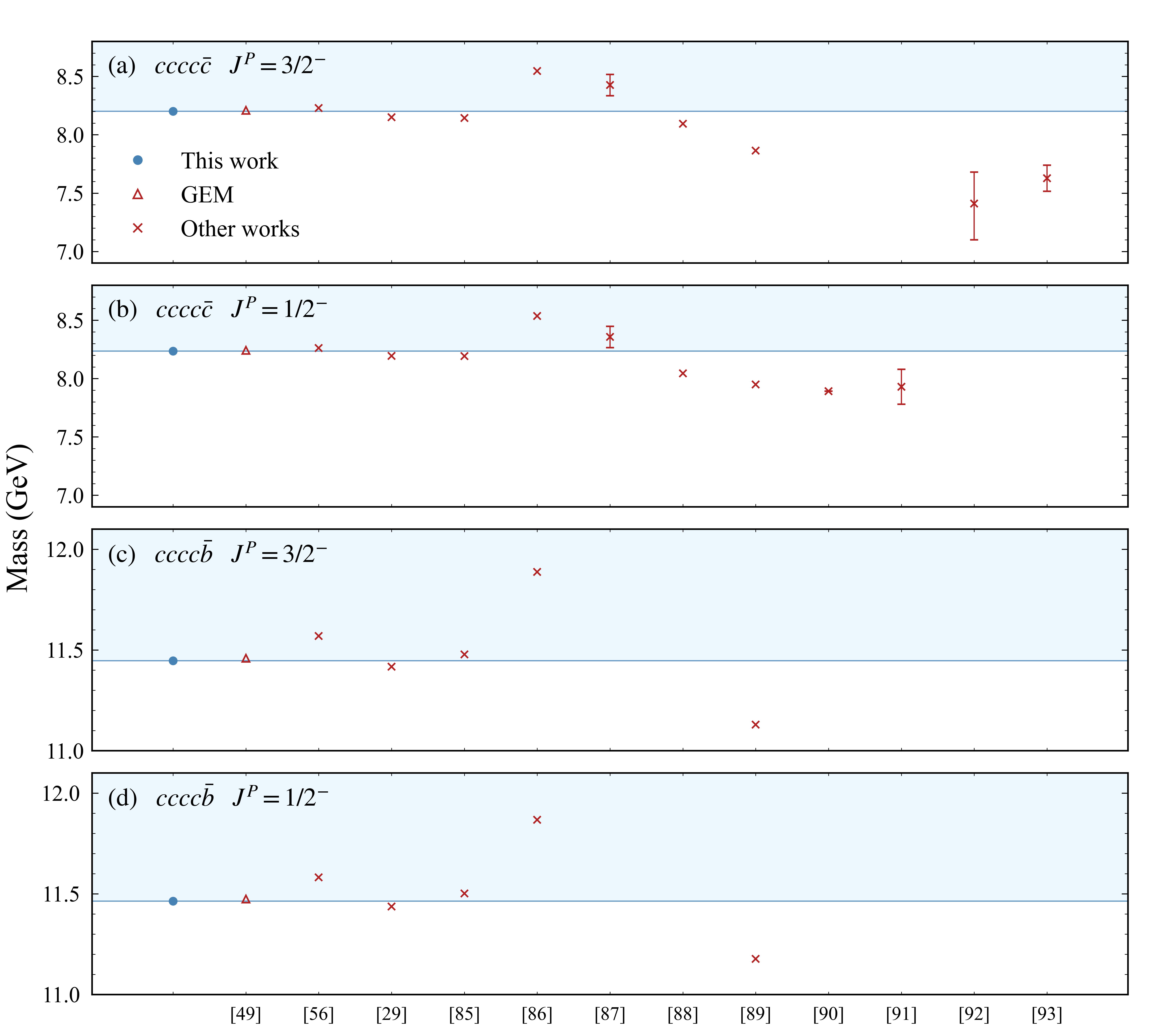
| This work | 8201.1(5) | 8235.5(7) | 11446.9(6) | 11463.4(6) |
| Ref. [49] | 8210 | 8242 | 11459 | 11474 |
| Ref. [56] | 8229 | 8262 | 11569 | 11582 |
| Ref. [29] | 8151 | 8194 | 11417 | 11437 |
| Ref. [85] | 8144.6 | 8193.2 | 11477.8 | 11501.5 |
| Ref. [86] | 8547.4 | 8537.4 | 11887.6 | 11867.7 |
| Ref. [87] | 8425.9(911) | 8356.9(910) | \(\cdots\) | \(\cdots\) |
| Ref. [88] | 8095 | 8045 | \(\cdots\) | \(\cdots\) |
| Ref. [89] | 7864 | 7949 | 11130 | 11177 |
| Ref. [90] | \(\cdots\) | 7892.3(4) | \(\cdots\) | \(\cdots\) |
| Ref. [91] | \(\cdots\) | 7930(150) | \(\cdots\) | \(\cdots\) |
| Ref. [92] | \(7410^{+270}_{-310}\) | \(\cdots\) | \(\cdots\) | \(\cdots\) |
| Ref. [93] | 7628(112) | \(\cdots\) | \(\cdots\) | \(\cdots\) |
1mm
In Figure 6, we present the mass spectra of these pentaquark states and compare them with the results from GEM. For the \(cccc\bar{c}\) system in Figure 6 (a), the masses of states \(J^P=3/2^-\) and \(J^P=1/2^-\) are lower than the GEM [49] predictions by approximately 6 to 9 MeV. For the \(cccc\bar{b}\) system in Figure 6 (b), the masses of states \(J^P=3/2^-\) and \(J^P=1/2^-\) are lower than the GEM predictions by approximately 10 to 12 MeV. For the \(bbbb\bar{b}\) system in Figure 6 (c), the masses of states \(J^P=3/2^-\) and \(J^P=1/2^-\) are lower than the GEM predictions by approximately 15 to 17 MeV. For the \(bbbb\bar{c}\) system in Figure 6 (d), the masses of states \(J^P=3/2^-\) and \(J^P=1/2^-\) are lower than the GEM predictions by approximately 12 MeV. The above comparisons show that for pentaquarks, the mass expectations from the NNQS remain systematically lower than GEM predictions. When the quark masses increase, the deviations grow, which means that the GEM performs better for charm systems than for bottom systems. It once again demonstrates that neural-network wave functions have stronger expressive power than GEM on multiquark wave functions.
Taking the \(cccc\bar{c}\) and \(cccc\bar{b}\) pentaquarks as examples, we compare our results with other model calculations in Table 9 and Figure 7. Our predicted masses are consistent with several recent calculations [29], [49], [56], [85], [88]. Specifically, they are slightly lower than the GEM results [49] and the MIT bag model [56], but slightly higher than those from the single Gaussian variational method [85], the DMC method [29], and the GEM combined with a complex-scaling approach [88]. In addition, our results are lower than the calculations based on the screened charge scheme [86] and the extended Gürsey–Radicati formalism [87]. On the other hand, our masses are significantly higher than those evaluated via the chromomagnetic interaction (CMI) model [89], the chiral quark model [90], and QCD sum rules [91]–[93]. These discrepancies largely originate from the different choices of the potentials employed in these models. Importantly, if the same potential were adopted, our variational approach would produce results closer to the true values, demonstrating its advantage in providing accurate predictions.
6 Summary↩︎
In this work, we propose a computational framework based on neural-network quantum states to calculate the mass spectra of fully‑heavy multiquark systems within a nonrelativistic quark model. The color‑spin wave functions are constructed exactly via \(\mathrm{SU}(3)\times \mathrm{SU}(2)\) group theory to enforce fermionic antisymmetry, while the spatial part is parameterized by deep neural networks. After benchmarking on conventional mesons and baryons—where NNQS reproduces or improves upon the Gaussian expansion method results—we compute the \(S\)-wave ground‑state masses of fully‑heavy tetraquarks and pentaquarks. Our approach consistently yields lower energies than GEM, a direct consequence of the variational principle, indicating that the neural network wave function offers greater expressive power by adaptively capturing nonperturbative many‑body spatial correlations without relying on restrictive a priori assumptions. Compared with traditional methods, NNQS overcomes the exponential growth of basis size and avoids the fermion sign problem, making it particularly suitable for high‑dimensional strongly correlated systems. Our results show good agreement with various model calculations, and importantly, when the same potential is employed, NNQS produces values closer to the true ones, demonstrating its superior accuracy and reliability. This framework not only provides a robust tool for the spectroscopy of exotic hadrons but also offers a flexible continuous‑space solver for investigating microscopic binding mechanisms. Future extensions to hexaquark and more complex systems are anticipated, which will further aid experimental searches for all‑heavy multiquark states.
7 Acknowledgments↩︎
We are grateful to Zi-Xiao Zhang, Hong-Fei Zhang and Jifeng Hu for code support, and to Xin-Yue Hu and Zhan-Wei Liu for valuable discussions on multiquark interactions. This work is partly supported by the National Natural Science Foundation of China with Grants Nos. 12375073, and 12547105.
References↩︎
Note that this does not mean a diquark-antidiquark approximation, but a way to combine to a color neutral object.↩︎