Automated residual plot assessment with the R package autovi and the Shiny application autovi.web
June 23, 2026
Abstract
Visual assessment of residual plots is a common approach for diagnosing linear models, but it relies on manual evaluation, which does not scale well and can lead to inconsistent decisions across analysts. The lineup protocol, which embeds the observed plot among null plots, can reduce subjectivity but requires even more human effort. In today’s data-driven world, such tasks are well-suited for automation. We present a new R package that uses a computer vision model to automate the evaluation of residual plots. An accompanying Shiny application is provided for ease of use. Given a sample of residuals, the model predicts a visual signal strength (VSS) and offers supporting information to help analysts assess model fit.
1 Introduction↩︎
Regression analysis is a widely used statistical modelling technique for data in many fields. There is a vast array of software for conducting regression modelling and generating diagnostics. The package lmtest [1] provides a suite of conventional tests, while the stats package [2] offers standard diagnostic plots such as residuals vs. fitted values, quantile-quantile (Q-Q) plots, and residuals vs. leverage plots. Additional packages like jtools [3], olsrr [4], rockchalk [5], and ggResidpanel [6] deliver similar graphical diagnostics, often with enhanced aesthetics or interactive features. These tools collectively produce the core diagnostic plots outlined in the classical text by [7]. The ecostats package [8] extends these diagnostics by incorporating simulation envelopes into residual plots. Meanwhile, DHARMa [9] compares empirical quantiles (0.25, 0.5, and 0.75) of scaled residuals to their theoretical counterparts, with a strong focus on identifying model violations such as heteroscedasticity, misspecified functional forms, and issues specific to generalised linear and mixed-effect models, like over/under-dispersion. It also provides conventional test annotations to reduce the risk of misinterpretation.
However, relying solely on subjective assessments of these plots can lead to issues such as over-interpreting random patterns as model violations. [10] demonstrated that visual inference methods, particularly those using the lineup protocol [11], offer more practical and reliable assessments of residual patterns than conventional tests, as they are less sensitive to minor departures. Packages such as nullabor [12], HLMdiag [13], and regressinator [14] support this approach by enabling users to compare observed residual plots with plots generated under null hypothesis, thereby helping to quantify the significance of any detected patterns.
As noted in [15], the lineup protocol has significant limitations in large-scale applications due to its reliance on human labour. To overcome this constraint, a computer vision model was developed alongside a corresponding statistical testing procedure to automate the assessment of residual plots. The model takes as input a residual plot and a set of auxiliary variables (such as the number of observations) and outputs a predicted visual signal strength (VSS). This VSS estimates the degree of deviation between the residual distribution of the fitted model and the reference distribution expected under correct model specification.
To make the statistical testing procedure and trained computer vision model widely accessible, we developed the R package autovi along with a companion web interface, autovi.web, which allows users to automatically assess their residual plots using the trained computer vision model.
The remainder of this paper is structured as follows: Section 2 introduces the definition and computation of visual signal strength. Section 3 expands on the computation of the null and bootstrapped residuals. Section 4 provides a detailed documentation of the autovi package, including its usage and infrastructure. Section 5 focuses on the autovi.web interface, describing its design and usage, along with illustrative examples. Finally, Section 6 presents the main conclusions of this work.
2 Definition and computation of visual signal strength↩︎
To train a computer vision model, a measure of the visible pattern in a plot is needed. We call this the visual signal strength (VSS), which measures how prominently a specific set of visual patterns appears in an image. This can be computed for a training set of data, and plots, where the generating distributions are specified.
In the context of classical normal linear regression model diagnostics, VSS describes the clarity of visual patterns on a diagnostic plot that may indicate model violations. Violations can be categorised as weak, moderate, or strong, but here we treat it as a continuous positive real variable. Importantly, its interpretation depends on how it is linked to a function of the data or the underlying data generating process. Consequently, the calculation of VSS can vary across different model classes or within the same model, depending on the generating function.
VSS estimates the distance between the residual distribution of a fitted classical normal linear regression model and a reference distribution [15]. The distance measure is based on the Kullback-Leibler (KL) divergence:
\[\label{eq:kl-0} D = \log\left(1 + D_{KL}\right),\tag{1}\]
where \(D_{KL}\) is given by:
\[\label{eq:kl-1} D_{KL} = \int_{\mathbb{R}^{n}}\log\frac{p(\hat{\boldsymbol{e}})}{q(\hat{\boldsymbol{e}})}p(\hat{\boldsymbol{e}})d\hat{\boldsymbol{e}},\tag{2}\]
here, \(\hat{\boldsymbol{e}}\) denotes the residual vector from the regression model, and \(p(\cdot)\) and \(q(\cdot)\) are the probability density functions of the reference residual distribution \(\mathrm{P}\) and the true residual distribution \(\mathrm{Q}\), respectively.
This distance measure depends on knowledge of the true residual distribution, which is unknown in practice. To compute \(D_{KL}\) for the training samples, Equation (2 ) takes different forms depending on the specific model violations. For instance, where necessary higher-order predictors, \(\boldsymbol{Z}\), and their corresponding parameter, \(\boldsymbol{\beta}_Z\), are omitted from the fitted linear model, the distance measure can be expanded as follows:
\[\label{eq:kl-2} D_{KL} = \frac{1}{2}\left(\boldsymbol{\mu}_z^\top(\text{diag}(\boldsymbol{R}\sigma^2))^{-1}\boldsymbol{\mu}_z\right),\tag{3}\]
where \(\boldsymbol{\mu}_z = \boldsymbol{R}\boldsymbol{Z}\boldsymbol{\beta}_z\), \(\boldsymbol{R} = \boldsymbol{I}_n - \boldsymbol{X}(\boldsymbol{X}^\top\boldsymbol{X})^{-1}\boldsymbol{X}^\top\) and \(\boldsymbol{X}\) is the design matrix of the regression model.
The computer vision model approximates this mapping from a set of residuals to its corresponding distance measure. It is trained on a large number of synthetic regression models, each designed to simulate specific violations of classical linear regression assumptions. These models incorporate non-linearity through Hermite polynomial transformations of predictors, heteroscedasticity by making the error variance a predictor-dependent function, and non-normality by drawing residuals from distributions such as discrete, uniform, and lognormal. Both simple and multiple linear regression structures are used, with controlled parameters to generate diverse and complex residual patterns. Since the data-generating process is known, the distance measure \(D\) can be explicitly calculated, enabling supervised training. The computer vision model takes a residual plot as input and outputs the corresponding distance measure, learning to quantify model violations directly from visual patterns. Additional details are provided in [15].
3 Definition and simulation of null and bootstrapped residuals↩︎
In the subsequent sections, we will frequently refer to null residuals and bootstrapped residuals, so it is helpful to first define and explain how they are generated.
Null residuals are used to generate null plots within the lineup protocol framework, serving as the foundation for the statistical testing in our automated residual plot assessment. Specifically, they represent residuals generated under the null hypothesis that the model is correctly specified. A common method for simulating null residuals in linear regression involves sampling from a normal distribution with mean zero and variance equal to the estimated variance of the error term. These simulated residuals and their corresponding plots depict what one would expect from a correctly specified model. If the true residual plot exhibits noticeable deviations from these null plots, it may suggest model misspecification.
Our computer vision model is trained to assign lower VSS to null plots and higher VSS to plots that display distinct patterns. Accordingly, statistical testing is performed by computing the proportion of null plots whose VSS equals or exceeds that of the observed residual plot. This proportion serves as a p-value for a one-sided hypothesis test.
Bootstrapped residuals are obtained by refitting the model on bootstrap samples, which are generated by sampling individual observations with replacement from the original dataset. The residual plots obtained from these refitted models are evaluated using the same computer vision model. The predicted VSS from the bootstrapped plots provide an empirical estimate of the variation in the VSS of the observed residual plot. By examining the proportion of bootstrapped plots that also exhibit significant violations, we can assess whether the original conclusion is robust to sampling variability.
4 R package: autovi↩︎
The main purpose of autovi is to provide rejection decisions and \(p\)-values for testing the null hypothesis (\(H_0\)) that the regression model is correctly specified. The package provides automated interpretation of residual plots using computer vision. The name autovi stands for automated visual inference. This functionality can be accessed through the R package autovi, or through a web interface, autovi.web, which enables users to perform analyses without installing R, Python, or their associated dependencies locally.
4.1 Motivation↩︎
Figure 1 shows three sets of plots of residuals against fitted values. The simulated example in (a) might be interpreted as a heteroscedastic pattern, however the automated reading would predict this to have a visual signal strength (VSS) of 1.53, with a corresponding \(p\)-value of 0.25. This means it would be interpreted as a good residual plot, that there is nothing in the data to indicate a violation of model assumptions. Skewness in the predictor variables is generating the apparent heteroscedasticity, where the smaller variance in residuals at larger fitted values is due to smaller sample size only. The Breusch–Pagan test [16] for heteroscedasticity would also not reject this as good residual plot.
The data in (b) is generated by fitting a linear model predicting mpg based on hp using the datasets::mtcars. It is a small data set, and there is a hint of nonlinear structure not
captured by the model. The automated plot reading would predict a VSS of 3.57, which has a \(p\)-value less than 0.05. That is, the nonlinear structure is most likely real, and indicates a problem with the model. The
conventional test, a Ramsey Regression Equation Specification Error Test (RESET) [17] would also strongly detect the nonlinearity.
The third example is generated using the surreal package [18], where structure residuals are embedded in the data. In this case, a quote inspired by Tukey, ‘visual summaries focus on unexpected values’, is used to define the residual structure. The automated plot reading predicts the VSS to be 5.87, with a \(p\)-value less than 0.05. Visually, the structure is strikingly clear, but a RESET test for nonlinear structure would not report a problem. (It would be detected by a Breusch–Pagan for heteroscedasticity and also Shapiro–Wilk test [19] for non-normality.)

Figure 1: Reading residual plots can be adifficult task, particularly for students new to statistical modelling.The autovi package makes it easier. Here are three examples ofresidual plots, which may appear to have structure. According to autovi,the visual signal strengths (VSS) of these three examples areapproximately (a) 1.53, (b) 3.57, (c) 5.87, resulting in (b), (c) beingsignificant violations of good residuals, but (a) is consistent with agood residual plot..
4.2 Implementation↩︎
The autovi package is built on the bandicoot object-oriented programming (OOP) system [20], marking a departure from R’s traditional S3 generic system. This OOP architecture enhances flexibility and modularity, allowing users to redefine key functions through method overriding.
The autovi infrastructure effectively integrates multiple programming languages and libraries into a comprehensive analytical tool. It relies on five core libraries from Python and R, each playing a critical role in the analysis pipeline. In Python, pillow [21] handles image processing tasks such as reading and resizing PNG files of residual plots, then converting them into input tensors for further analysis. TensorFlow [22], a key component of modern machine learning, is used to predict the VSS of these plots using a pre-trained convolutional neural network.
In the R environment, autovi utilizes several libraries. ggplot2 [23] generates the initial residual plots, saved as PNG files for visual input. cassowaryr [24] computes scagnostics (scatter plot diagnostics), providing numerical features that capture statistical properties of the plots. These scagnostics complement the visual analysis by offering quantitative metrics as secondary input to the computer vision model. reticulate [25] enables seamless communication between R and Python.
4.3 Installation↩︎
The autovi package is available on CRAN. It is actively developed and maintained, with the latest updates accessible on GitHub. This paper uses autovi version 0.4.2. The package includes
internal functions to check the current Python environment used by the reticulate package. If the necessary Python packages are not installed in the Python interpreter, an error will be raised. If you want to select a specific Python environment, you can do so by calling the reticulate::use_python()
function before using the autovi package.
We recommend using the Shiny application autovi.web if users encounter installation problems.
4.4 Usage↩︎
4.4.1 Numerical summary↩︎
Three steps are needed to get an automated assessment of a set of residuals and fitted values:
Load the autovi package using the
library()function.Create a checker object with a linear regression model.
Call the
check()method of the checker, which, by default, predicts the VSS for the true residual plot, 100 null plots, and 100 bootstrapped plots. The method stores the predictions internally and prints a concise results report.
The code to do this is:
It produces the following summary:
<AUTO_VI object>
 Status:
  - Fitted model: lm
  - Keras model: (None, 32, 32, 3) + (None, 5) -> (None, 1)
     - Output node index: 1
  - Result:
     - Observed visual signal strength: 3.16 (p-value = 0.0396)
     - Null visual signal strength: [100 draws]
        - Mean: 1.274
        - Quantiles:
           ╔══════════════════════════════════════════╗
           ║  25           ║0.802 1.111 1.575 1.666 1.919 2.657 3.348 ║
           ╚══════════════════════════════════════════╝
     - Bootstrapped visual signal strength: [100 draws]
        - Mean: 2.795 (p-value = 0.05941)
        - Quantiles:
           ╔══════════════════════════════════════════╗
           ║  25           ║2.455 2.941 3.177 3.300 3.474 3.537 3.668 ║
           ╚══════════════════════════════════════════╝
     - Likelihood ratio: 0.7333 (boot) / 0.06284 (null) = 11.67
The summary includes observed VSS of the true residual plot and associated \(p\)-value of the automated visual test. The \(p\)-value is the proportion of null plots (out of the total 100) that have VSS greater than or equal to that of the true residual plot. The report also provides sample quantiles of VSS for null samples and bootstrapped data plots, providing more information about the sampling variability and a likelihood of model violations. The likelihood is computed from the proportion of values greater than the observed VSS in both the bootstrapped data values and the simulated null values.
4.4.2 Visual summary↩︎
Users can visually inspect the original residual plot alongside a sample null plot using plot_pair() or a lineup of null plot plot_lineup(). This visual comparison can clarify why \(H_0\) is
either rejected or not, and help identify potential remedies.

Figure 2: True plot alongside one null plot, forquick comparison..
The plot_pair() method (Figure 2) displays the true residual plot on the left and a single null plot on the right. If a full lineup was shown, the true residual plot would be embedded in a page of null
plots. Users should look for any distinct visual patterns in the true residual plot that are absent in the null plot. Running these functions multiple times can help any visual suspicions, as each execution generates new random null plots for
comparison.
The package offers a straightforward visualisation of the assessment result through the summary_plot() function.
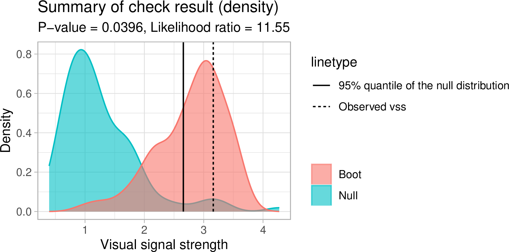
Figure 3: Summary plot comparing the densities ofVSS for bootstrapped residual samples (red) relative to VSS for nullplots (blue)..
In the result, shown in Figure 3, the blue area represents the density of VSS for null residual plots, while the red area shows the density for bootstrapped residual plots. The dashed line indicates the VSS of the true residual plot, and the solid line marks the critical value at a 95% significance level. The \(p\)-value and the likelihood ratio are displayed in the subtitle. The likelihood ratio represents the ratio of the likelihood of observing the VSS of the true residual plot from the bootstrapped distribution compared to the null distribution.
Interpreting the plot involves several key aspects. If the dashed line falls to the right of the solid line, it suggests rejecting the null hypothesis. The degree of overlap between the red and blue areas indicates similarity between the true residual plot and null plots; greater overlap suggests more similarity. Lastly, the portion of the red area to the right of the solid line represents the percentage of bootstrapped models considered to have model violations.
This visual summary provides an intuitive way to assess the model’s fit and potential violations, allowing users to quickly grasp the results of the automated analysis.
4.5 Modularized infrastructure↩︎
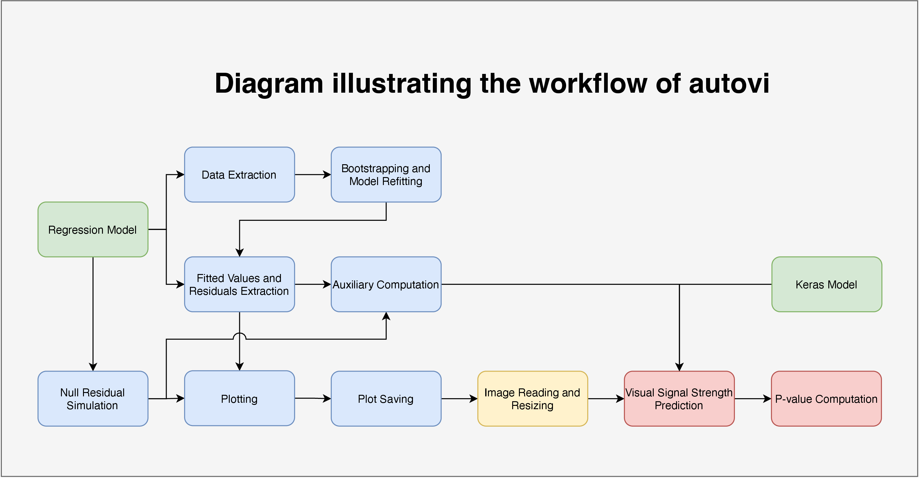
Figure 4: Diagram illustrating the infrastructureof the R package autovi. The modules in green areprimary inputs provided by users. Modules in blue are overridablemethods that can be modified to accommodate users’ specific needs. Themodule in yellow is a pre-defined non-overridable method. The modules inred are primary outputs of the package..
The initial motivation for developing autovi was to create a convenient interface for sharing the models described and trained in [15]. However, recognising that the classical normal linear regression model represents a restricted class of models, we sought to avoid limiting the potential for future extensions, whether by the original developers or other developers. As a result, the package was designed to function seamlessly with linear regression models with minimal modification and few required arguments, while also accommodating other classes of models through partial infrastructure substitution. This modular and customisable design allows autovi to handle a wide range of residual diagnostics tasks.
The infrastructure of autovi consists of ten core modules: data extraction, bootstrapping and model refitting, fitted values and residuals extraction, auxiliary computation, null residual simulation, plotting, plot saving, image reading and resizing, VSS prediction, and \(p\)-value computation. Each module is designed with minimal dependency on the preceding modules, allowing users to customise parts of the infrastructure without affecting its overall integrity. An overview of this infrastructure is illustrated in Figure 4.
The package takes regression models and a Keras model as primary inputs. Modules for VSS prediction and \(p\)-value computation are fixed but accessible via function arguments, using TensorFlow for inference and statistical testing. The image loading module is also fixed, using PIL to read and resize images based on the Keras model’s input shape.
The remaining seven modules are overridable, allowing users to adapt the workflow as needed. The data extraction module extracts a data.frame containing variables used in the regression model. The bootstrapping and refitting module resamples
the data and refits the model. The fitted values and residuals extraction module returns these values as a data.frame. The auxiliary computation module calculates scagnostics such as monotonicity. The plotting module generates a
ggplot in a standard format, and the plot saving module exports it at the same resolution as the training images. These modules are described in detail in the package documentation.
4.6 Extension to other model classes↩︎
The autovi R package can be extended to accommodate other classes of models beyond linear regression, such as generalised linear models (glm). This is achieved by substituting
the relevant overridable modules, and if needed, supplying a different Keras model.
We provide an example of defining a new checker class tailored for Poisson regression using the glm framework:
Define a new class using
new_class()withAUTO_VIas the parent class.Override the necessary methods using
register_method(). In this example, we use Pearson residuals. To simulate null residuals, we assume the fitted model is correct and the estimated coefficients are accurate. New response values are generated accordingly, and a new model is fitted to this simulated response. Null residuals are then extracted from this refitted model.Create an alias for the
instantiate()method of the new class.
The resulting checker class can be employed analogously to the linear model case described in Section 4.4. For illustration, we fit a Poisson model in which the quadratic term of the predictor \(x\) is intentionally omitted. This misspecification manifests as a pronounced U-shaped pattern in the lineup display (see Figure 5), which is also successfully identified by the computer vision model, yielding a p-value substantially below the conventional threshold of 0.05.
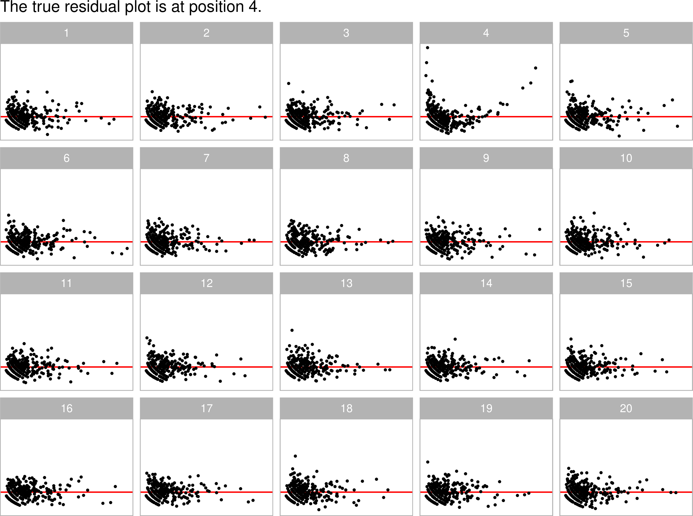
Figure 5: A lineup of residual plots from Poissongeneralised linear models, with the true residual plot at position 4,which displays a distinct U-shaped pattern. In contrast, the null plotsshow characteristics broadly consistent with well-behaved residuals fromlinear regression models..
<AUTO_POIS_VI object>
 Status:
  - Fitted model: glm, lm
  - Keras model: (None, 32, 32, 3) + (None, 5) -> (None, 1)
     - Output node index: 1
  - Result:
     - Observed visual signal strength: 4.875 (p-value = 0.009901)
     - Null visual signal strength: [100 draws]
        - Mean: 1.331
        - Quantiles:
           ╔══════════════════════════════════════════╗
           ║  25           ║1.035 1.233 1.488 1.644 1.941 2.276 2.639 ║
           ╚══════════════════════════════════════════╝
     - Bootstrapped visual signal strength: [100 draws]
        - Mean: 5.51 (p-value = 0.009901)
        - Quantiles:
           ╔══════════════════════════════════════════╗
           ║  25           ║5.330 5.505 5.698 5.735 5.830 5.903 6.013 ║
           ╚══════════════════════════════════════════╝
     - Likelihood ratio: 0.05096 (boot) / 0 (null) = Extremely large
It is important to note, however, that the pre-trained computer vision model included in autovi, such as vss_phn_32 (see list_keras_models() for the full list of available models), was developed
specifically for diagnostics of linear regression. Its applicability to other model classes relies on the assumption that the null residual plots exhibit characteristics broadly consistent with those of well-behaved linear regression residuals, that is,
residuals should be approximately randomly scattered around zero, display roughly constant variance across the range of fitted values, and exhibit no discernible structure or curvature. If these conditions are not met, or if model violations do not give
rise to visually detectable patterns, the validity of the automated diagnostics may be compromised. In such cases, users are encouraged to train and apply their own Keras models. Detailed guidance on model training and
discussion on extending the methodology to other model classes can be found in [15].
5 Web interface: autovi.web↩︎
The autovi.web Shiny application extends the functionality of autovi by offering a user-friendly web interface for automated residual plot assessment. This eliminates the common challenges associated with software installation, so users can avoid managing Python environments or handling version requirements for R libraries. The platform is cross-platform and accessible on various devices and operating systems, making it suitable even for users without R programming experience. Additionally, updates are managed centrally, ensuring that users always have access to the latest features. This section discusses the implementation based on autovi.web version 0.1.0.
5.1 Implementation↩︎
The interface autovi.web is built using the shiny [26] and shinydashboard [27] R packages. Hosted on the shinyapps.io domain, the application is accessible through any modern web browser. The R packages htmltools [28] and shinycssloaders [29] are used to render markdown documentation in Shiny application, and for loading animations for Shiny widgets, respectively.
Determining the best way to implement the backend was difficult. In our initial planning for autovi.web, we considered implementing the entire web application using the webr framework [30], which would have allowed the entire application to run directly in the user’s browser. However, webr does not support packages which use compiled Fortran code, which is required by splancs [31], a dependency of autovi. In the future, it is possible that a working Emscripten [32] version of this package may allow full webr support.
We also explored the possibility of implementing the web interface using frameworks built on other languages, such as Python. However, server hosting domains that natively support Python servers typically do not have the latest version of R installed. Additionally, calling R from Python is typically done using the rpy2 Python library [33], but this approach can be awkward when dealing with language syntax related to non-standard evaluation. Another option we considered was renting a server where we could have full control, such as those provided by cloud platforms like Google Cloud Platform (GCP) or Amazon Web Services (AWS). However, deploying and maintaining the server securely requires some expertise. Ultimately, the most practical solution was to use the shiny and shinydashboard frameworks, which are well-established in the R community and offer a solid foundation for web application development.
The server-side configuration of autovi.web is carefully designed to support its functionality. Most required Python libraries, including pillow and numpy, are pre-installed on the server. These libraries are integrated into the Shiny application using the reticulate package, which provides an interface between R and Python.
Due to shinyapps.io’s resource policy, inactive servers enter sleep mode, clearing the local Python environment. When reactivated for a new session, libraries must be reinstalled. While this ensures a clean environment for each session, it may lead to slightly longer loading times for the first user after a period of inactivity.
In contrast to autovi, autovi.web leverages TensorFlow.js, a JavaScript library that allows the execution of machine learning models directly in the browser. This choice enables native browser execution, enhancing compatibility across different user environments, and shifts the computational load from the server to the client-side. TensorFlow.js also offers better scalability and performance, especially when dealing with resource-intensive computer vision models on the web.
While autovi requires downloading the pre-trained computer vision models from GitHub, these models in ‘.keras’ file format are incompatible with TensorFlow.js. Therefore, we extract and store the model weights in JSON files and include them as extra resources in the Shiny application. When the application initialises, TensorFlow.js rebuilds the computer vision model using these pre-stored weights.
To allow communication between TensorFlow.js and other components of the Shiny application, the shinyjs R package [34] is used. This package allows calling custom JavaScript code within the Shiny framework. The specialised JavaScript code for initialising TensorFlow.js and calling TensorFlow.js for VSS prediction is deployed alongside the Shiny application as additional resources.
5.2 Usage↩︎
The workflow of autovi.web is designed to be straightforward, with numbered steps displayed in each panel. There are two example datasets provided by the web application. The single residual plot example uses the
dino dataset from the R package datasauRus [35]. The lineup example uses
residuals from a simulated regression model that has a non-linearity issue. We walk through the lineup example to further demonstrate the workflow of the web application.
5.2.1 Reading data and setting parameters↩︎
The user can select to upload data as either a single set of residuals and fitted values in a two (or more) column CSV file or a pre-computed lineup of residuals and null datasets in a three (or more) column CSV file (i.e. multiple sets of residuals and
fitted values with a column indicating the set label). Here we illustrate use with lineup example data sets (Figure 6). To use the lineup example data, click the ‘Use Lineup Example’ button. The data status will then
update to show the number of rows and columns in the dataset, and the CSV type will automatically be selected to the correct option. Since the example dataset follows the variable naming conventions assumed by the web application, the columns for fitted
values, residuals, and labels of residual plots are automatically mapped such that the column named as .fitted is mapped to fitted values, .resid is mapped to residuals and if applicable, .sample to labels of the
residual set (middle image). If the user is working with a custom dataset, these options must be set accordingly. Whenever a data containing a lineup, the user must manually select the label for the true residual plot, otherwise the web application does
not provide all the results. The last step is to click the play button (right image) to start the assessment.
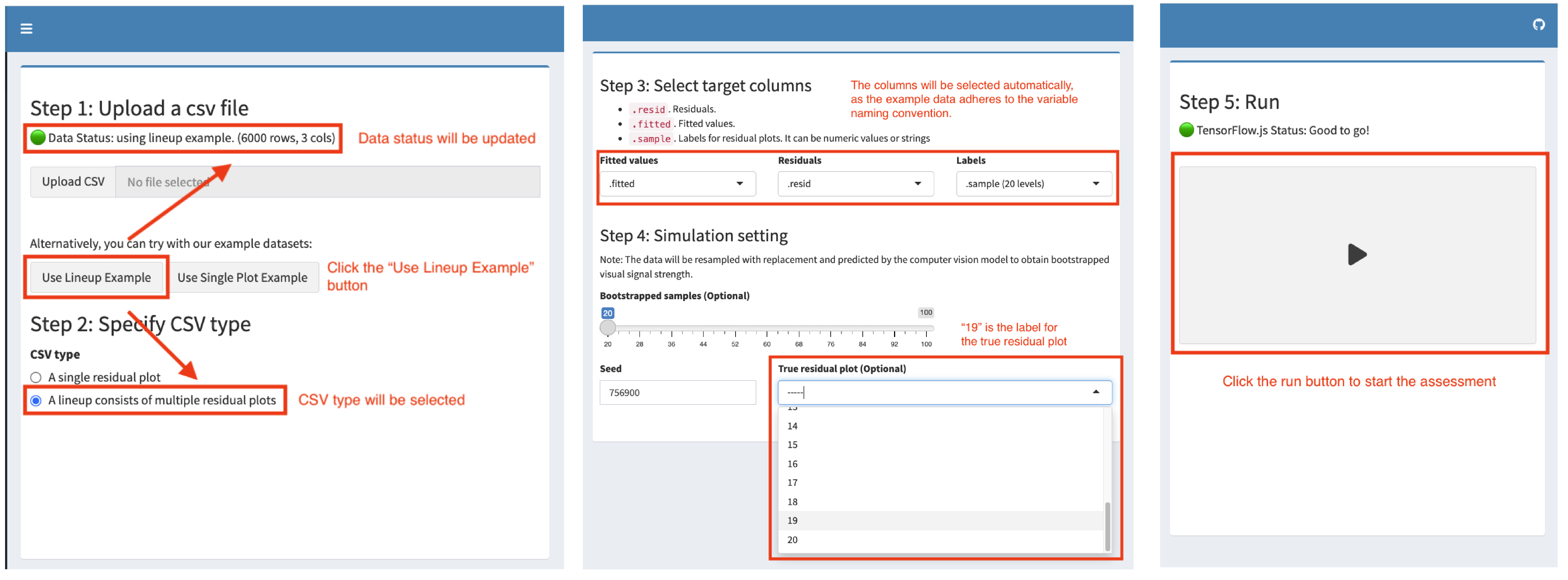
Figure 6: To begin the workflow forautovi using the lineup example dataset, the user clicks the’Use Lineup Example’ button (left) to load the example dataset, duringwhich the data status and CSV type will be automatically updated. Theuser must manually select the label for the true residual plot (middle)to compute further results. The user initiates the assessment of thelineup example data by clicking the run button (right)..
5.2.2 Results provided↩︎
Results are provided in multiple panels. The first row of the table Figure 7 is the most crucial to check, as it provides the VSS and the rank of the true residual plot among the other plots. The summary text beneath the table provides the \(p\)-value, which can be used for quick decision-making. The lineup is for manual inspection, and the user should see if the true residual plot is visually distinguishable from the other plots, to confirm if the model violation is serious.
The density plot in Figure 8 offers a more robust result, allowing the user to compare the distribution of bootstrapped VSS with the distribution of null VSS. Finally, the grayscale attention map (right image) can be used to check if the target visual features, like the non-linearity present in the lineup example, are captured by the computer vision model, ensuring the quality of the assessment. The attention map is the gradient of the model output with respect to the grayscale image input, indicating the sensitivity of the output to each pixel.
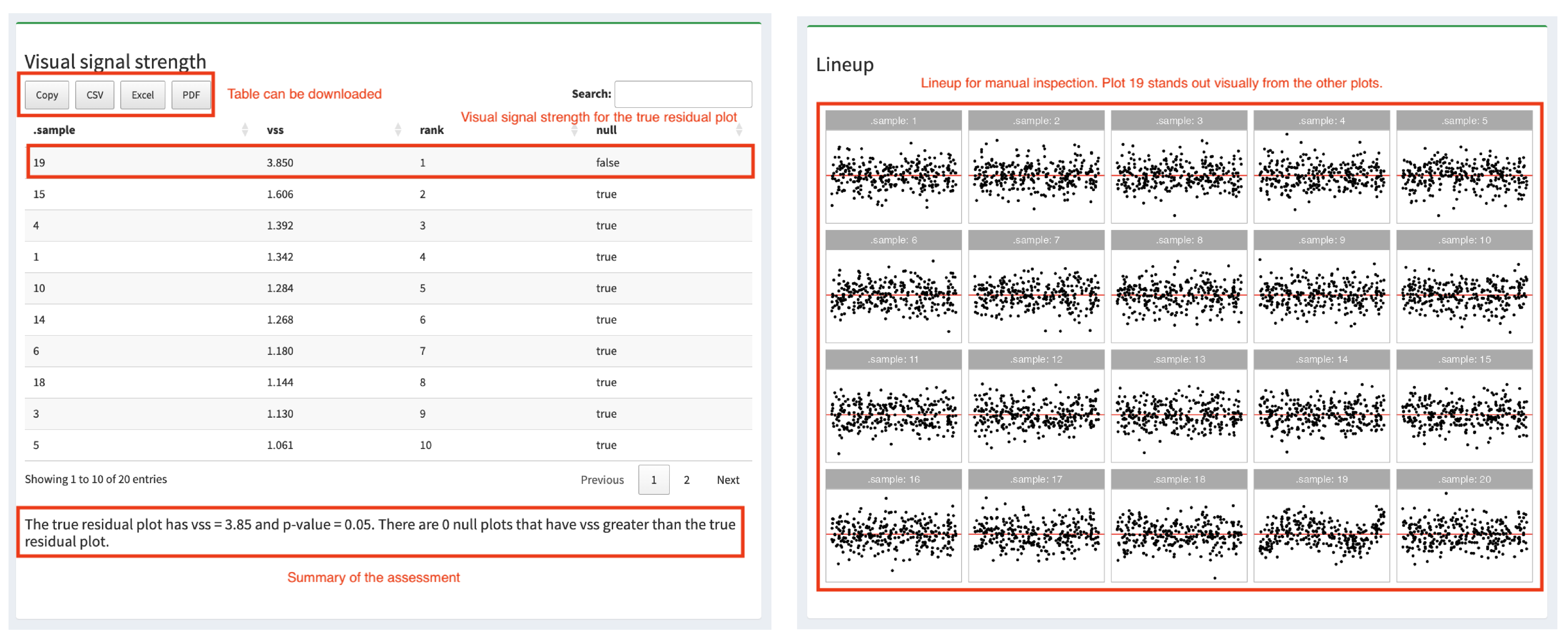
Figure 7: Results for the lineup. The VSS ofthe true residual plot is displayed in the first row of the table of VSSvalues for all the null plots (left image), with a summary text beneaththe table providing the \(p\)-value to aid in decision-making. A lineupof residual plots allows for manual inspection (right image)..

Figure 8: Summaries assessing thestrength of the pattern and which elements of the plot contribute. Thedensity plot helps verify if the bootstrapped distribution differs fromthe null distribution (left image). The attention map (right image)offers insights into whether the computer vision model has captured theintended visual features of the true residual plot..
6 Conclusions↩︎
This paper presents new regression diagnostics software, the R package autovi and its accompanying web interface, autovi.web. It addresses a critical gap in the current landscape of statistical software. While regression tools are widely available, effective and efficient diagnostic methods have lagged behind, particularly in the field of residual plot interpretation.
The autovi R package, introduced in this paper, automates the assessment of residual plots by incorporating a computer vision model, reducing reliance on time-consuming and potentially inconsistent human interpretation. This automation improves the efficiency of the diagnostic process and promotes consistency in model evaluation across different users and studies.
The development of the accompanying Shiny app, autovi.web, expands access to these advanced diagnostic tools, by providing a user-friendly interface. It makes automated residual plot assessment accessible to a broader audience, including those who may not have extensive programming experience. This web-based solution effectively addresses the potential barriers to adoption, such as complex dependencies and installation requirements, that are often associated with advanced statistical software.
The combination of autovi and autovi.web offers a comprehensive solution to the challenges of residual plot interpretation in regression analysis. These tools have the potential to significantly improve the quality and consistency of model diagnostics across various fields, from academic research to industry applications. By automating a critical aspect of model evaluation, they allow researchers and analysts to focus more on interpreting results and refining models, rather than grappling with the intricacies of plot assessment.
The framework established by autovi and autovi.web opens up exciting possibilities for further research and development. Future work could explore the extension of these automated assessment techniques to other types of diagnostic plots and statistical models, potentially revolutionising how we approach statistical inference using visual displays more broadly.
7 Resources and supplementary material↩︎
The current version of autovi can be installed from CRAN, and source code for both packages are available at github.com/TengMCing/autovi and github.com/TengMCing/autovi_web respectively. The web interface is available from autoviweb.netlify.app.
This paper is reproducibly written using Quarto [36] powered by Pandoc [37] and pdfTeX. The full source code to reproduce this paper is
available at github.com/TengMCing/autovi_paper.
These R packages were used for the work: tidyverse [38], lmtest [1], kableExtra [39], patchwork [40], rcartocolor [41], glue [42], here [43], magick [44], yardstick [45] and reticulate [25].