Initial-state-dependent dephasing effect in non-Hermitian Su-Schrieffer-Heeger models
June 23, 2026
Abstract
Understanding the dynamical evolution of non-Hermitian systems under extra external dissipation is essential for devising non-Hermitian quantum information devices that surpass the capabilities of their Hermitian counterparts. Dephasing, a major realistic dissipation, is conventionally considered detrimental to information processing. However, its impact on non-Hermitian systems remains largely unexplored. Here, we focus on finite-sized non-Hermitian Su-Schrieffer-Heeger (SSH) lattice models with alternating gain and loss in real space and examine the dynamical evolution of the trace distance under pure dephasing. By tuning system parameters, this model supports phases with either parity-time or anti-parity-time symmetries, enabling us to explore the interplay between dephasing and different non-Hermitian symmetries within a single platform. While the trace distance exhibits distinct dynamical behaviors across the different phases in the absence of dephasing, its response to dephasing is largely symmetry-independent but instead initial-state dependent. By varying initial states with excitations initialized on different sites, we observe that increasing the dephasing strength can either merely accelerate the decay of the trace distance or stabilize it. Interestingly, we reveal two kinds of dephasing-induced stabilization that differ in the strong dephasing limit: a partial stabilization, where the trace distance approaches a finite value smaller than its initial value in the long-time limit, and a complete stabilization, where the trace distance remains at its initial value throughout the entire evolution. By analyzing the equation of motion, we attribute the initial-state dependent dephasing effect to the alternating gain and loss in the system and confirm its absence in Hermitian counterparts. Furthermore, in the anti-parity-time symmetry unbroken phase, we identify a continuous suppression–upon increasing the dephasing strength–of the otherwise exponential decay of the trace distance seen in the absence of dephasing, marking an unconventional dephasing-induced protection against information loss. Our findings, extendable to any state-based information-theoretic quantity, reveal the intricate dynamical response of non-Hermitian SSH models to dephasing, thereby facilitating their potential information-processing applications.
1 Introduction↩︎
Non-Hermitian quantum mechanics has emerged as a transformative framework, extending the boundaries of traditional quantum theory beyond the constraints of Hermiticity [1]–[6]. Unlike their Hermitian counterparts, non-Hermitian systems exhibit unique spectral features, most notably the appearance of exceptional points (EPs) where eigenvalues and eigenvectors coalesce [7]–[13]. By marking the points of spectral reconfiguration, EPs usually define the transition points between symmetry-unbroken and symmetry-broken regimes. This spectral flexibility facilitates the emergence of unconventional symmetries such as parity-time (\(\mathcal{PT}\)) and anti-parity-time (\(\mathcal{APT}\)) symmetries [6], [10], [14]–[26]. A typical approach to constructing non-Hermitian systems with certain symmetries is the introduction of gain and loss into conventional Hermitian systems [27]–[38]. Serving as a quintessential example of this paradigm, the integration of non-Hermiticity into the Su-Schrieffer-Heeger (SSH) model [39] has emerged as a focal point of contemporary research [18], [40]–[58]. Particularly, recent studies have further extended non-Hermitian SSH model to incorporate long-range hopping [49], higher periodicity [59], [60], nonlinearity [61], [62] and even many-body interactions [63], [64].
The exotic static properties of non-Hermitian systems suggest their potential for unique functionalities in quantum information-processing [65]–[68]. Fully harnessing this potential, however, necessitates a shift in focus toward their dynamical behaviors [22], [25], [69]–[76]. Given that experimentally realized non-Hermitian systems are typically effective systems that remain open to surrounding environments [10], [26], [66], [77], [78], the impact of environmental dissipation on their dynamical properties must be carefully characterized [75], [79]–[81]. In practical quantum information processing, dephasing is a ubiquitous and typically detrimental source of noise that leads to the loss of information. While dephasing usually accelerates the decay of quantum information in Hermitian systems, its role in non-Hermitian systems might be fundamentally different due to the nontrivial spectral structure. Recent studies have hinted that the combination of non-Hermiticity and dissipation can lead to counterintuitive effects, such as decoherence-induced EPs [78]. Understanding how the dynamical signatures of \(\mathcal{PT}\) and \(\mathcal{APT}\) symmetries persist or evolve under dephasing is therefore crucial for both fundamental physics and the design of robust non-Hermitian quantum devices.
In this work, we investigate non-Hermitian SSH lattice models with alternating gain and loss in real space, subject to local pure dephasing. Crucially, by simply tuning system parameters, this non-Hermitian lattice model hosts three distinct phases: the \(\mathcal{PT}\)-unbroken, \(\mathcal{APT}\)-unbroken and symmetry broken phases. This versatility allows us to explore the interplay between various non-Hermitian symmetries and dephasing within a unified platform. In contrast to previous studies on non-Hermitian SSH models, which typically analyze the corresponding Bloch Hamiltonian in momentum space under the assumption of a perfect periodicity in real space–a condition often challenging to realize in real-space experiments, we work directly with finite-sized lattice systems in real space. Consequently, our results correspond directly to the system under consideration, thereby facilitating direct experimental verification.
Serving as benchmarks for isolating the dynamical responses of non-Hermitian SSH models to dephasing, we first characterize the dynamical signatures of three phases as imprinted on the evolution of the trace distance [82], which is an information-theoretic quantity that quantifies the information flow [22], [71], [75]. We show that the dynamics of the trace distance exhibits persistent oscillation, damped oscillation and superpositions of exponential decays in the \(\mathcal{PT}\)-unbroken, symmetry broken and \(\mathcal{APT}\)-unbroken phases, respectively. These distinct behaviors originate from the differences in the Hamiltonian spectrum across the different phases.
Turning to open non-Hermitian SSH models subject to dephasing, we adopt a generalized quantum Lindblad master equation [75], [80], [83], [84] to describe the dynamics of the normalized system density matrix. Interestingly, we find that the basic trends of the dynamical evolution of the trace distance under varying dephasing strengths remain almost the same across different phases and are sensitive only to the initial state. By varying initial states with a single excitation initialized on different sites, we observe two basic effects of dephasing: one where dephasing merely accelerates the decay of the trace distance, playing a detrimental role similar to its impact on Hermitian systems, and another where dephasing stabilizes the trace distance in the strong-dephasing limit. Notably, this dephasing-induced stabilization occurs in two forms: partial stabilization, where the trace distance approaches a finite value smaller than its initial value in the long-time limit under strong dephasing, and complete stabilization, where the dynamical evolution of the trace distance is completely frozen in the strong-dephasing limit such that the trace distance remains at its initial value. By exploiting the equation of motion for the density matrix elements in the strong-dephasing limit, we attribute the initial-state dependence of the dynamical response to dephasing to the model feature of alternating gain and loss in real space, as initial excitations starting from sites with gain versus loss lead to distinct dynamics. Moreover, by examining the trend toward complete stabilization upon increasing the dephasing strength, we identify an unusual dynamical response of the non-Hermitian SSH model in the \(\mathcal{APT}\)-symmetry-unbroken phase: a continuous suppression upon increasing the dephasing strength is observed, which is absent in other phases and in its Hermitian counterpart. We explain this continuous suppression via the Liouvillian gap, thereby marking a beneficial role of dephasing in protecting information.
The structure of the paper is organized as follows. In Sec. 2, we introduce a minimal four-site non-Hermitian SSH lattice model with alternating gain and loss in real space and determine its phase diagram through a comprehensive symmetry analysis. We also present the evolution dynamics of the trace distance in the absence of dephasing for later comparison. In Sec. 3, we explore the dynamical behaviors of the trace distance under pure dephasing. By combining analytical equation-of-motion analysis with extensive numerical simulations, we provide an in-depth analysis of the initial-state-dependent dynamical response to dephasing. In Sec. 4, we further demonstrate the robustness of our findings in a multi-site non-Hermitian SSH lattice. Finally, we summarize the study in Sec. 5.
2 Non-Hermitian SSH model: Phase diagram and closed-system dynamics↩︎
2.1 Model setup↩︎
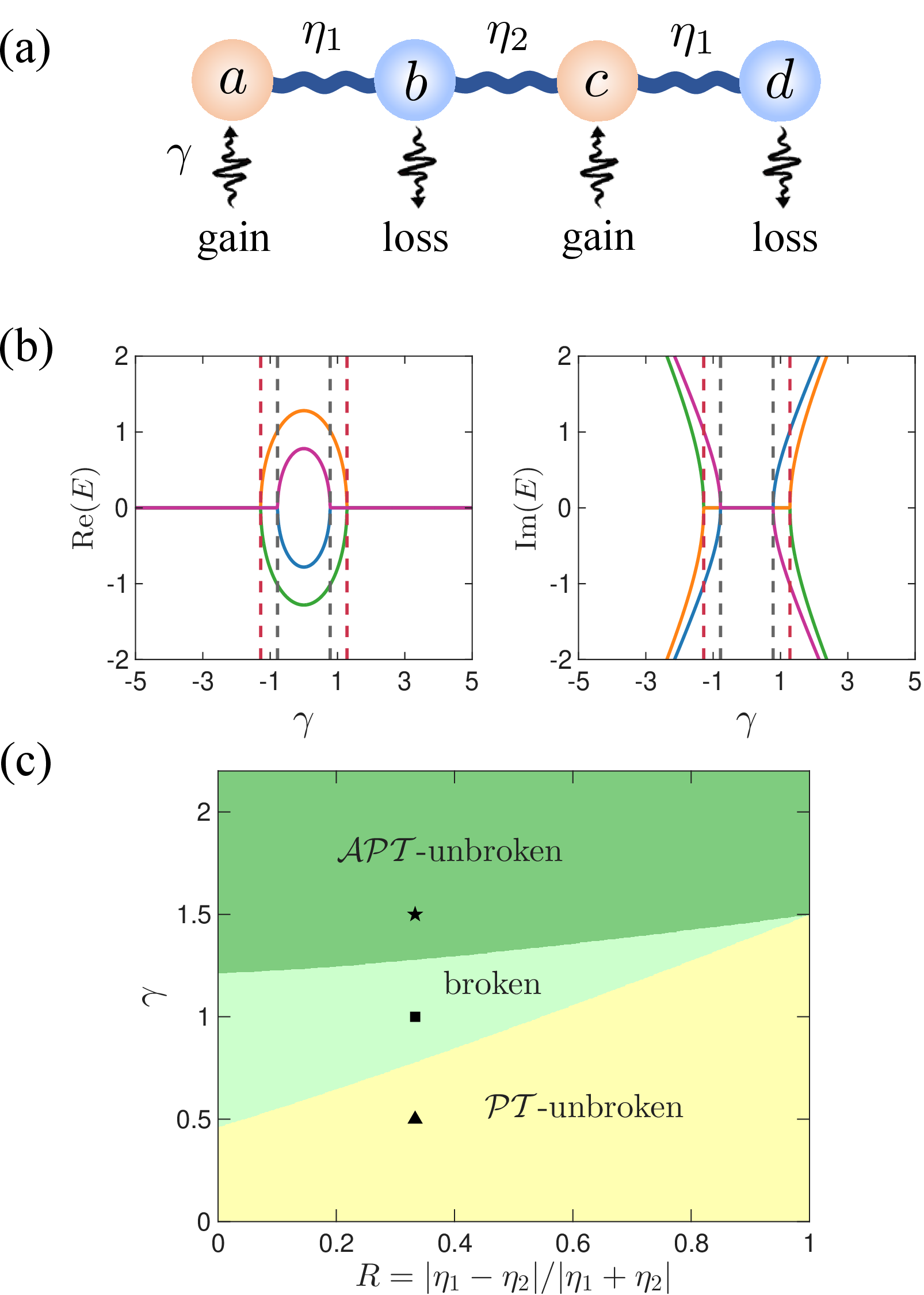
We consider a minimal one-dimensional non-Hermitian SSH lattice model that is not only simple to analyze and amenable to analytical treatment but also exhibits rich dynamical behaviors, allowing us to demonstrate the essential physics underlying the interplay between non-Hermiticity and dephasing. This minimal model, schematically illustrated in Fig. 1 (a), consists of four sites and is described by the Hamiltonian \[\begin{align} \hat{H} =& \eta_1(\hat{a}^\dagger \hat{b} + \hat{c}^\dagger \hat{d} + \rm{H.c.}) + \eta_2(\hat{b}^\dagger \hat{c} + \rm{H.c.}) \nonumber\\ &+ i\gamma(\hat{a}^\dagger \hat{a} - \hat{b}^\dagger \hat{b} + \hat{c}^\dagger \hat{c} - \hat{d}^\dagger \hat{d}), \label{erci} \end{align}\tag{1}\] where \(\hat{a}, \hat{b}, \hat{c}\) and \(\hat{d}\) denote the annihilation operators (with the corresponding creation operators implied) of the first, second, third and fourth sites (see Fig. 1 (a)), respectively. ‘H.c.’ is short for Hermitian conjugate, and \(\eta_{1,2}\) represent the alternating inter-site coupling strengths. Unless otherwise stated, we set \(\eta_1\neq \eta_2\). We consider balanced gain and loss, with a single parameter \(\gamma\) controlling the strength of the alternating gain and loss processes applied to the sites and thus quantifying the degree of non-Hermiticity. Throughout this study, we consider open boundary conditions.
Notably, the minimal model we consider functions as a fundamental unit cell for constructing extended multi-site non-Hermitian SSH lattice models [47], [52], [54], [55]. In Sec. 4, we will use this extension strategy to study a multi-site system, but prior to that section we focus on this minimal system. In contrast to existing studies that typically analyze the Bloch Hamiltonian in momentum space that inherently requires an infinite number of unit cells in real space, we work directly with finite-sized non-Hermitian SSH lattice models in real space. This choice offers two benefits. First, the system is amenable to implementation in current finite-sized experimental platforms. Second, the obtained results accurately reflect the properties of the specific real-space system, which is also important for experimental verification.
We restrict our analysis to the single-excitation subspace spanned by the Fock states \(\{|S_1\rangle, |S_2\rangle, |S_3\rangle, |S_4\rangle\}\), where \(|S_1\rangle = |1000\rangle\), \(|S_2\rangle = |0100\rangle\), \(|S_3\rangle = |0010\rangle\) and \(|S_4\rangle = |0001\rangle\), with \(|S_n\rangle\) representing an excitation on the \(n\)th site and all other sites empty. In this basis, the Hamiltonian in Eq. (1 ) is explicitly given by the following \(4\times 4\) matrix \[\begin{align} \hat{H} = \begin{pmatrix} i\gamma & \eta_1 & 0 & 0 \\ \eta_1 & -i\gamma & \eta_2 & 0 \\ 0 & \eta_2 & i\gamma & \eta_1 \\ 0 & 0 & \eta_1 & -i\gamma \end{pmatrix}. \label{eq1} \end{align}\tag{2}\]
2.2 Spectrum and phase diagram↩︎
Before proceeding to the dynamics, we first analyze the spectrum and symmetry properties of the model. Using the matrix form in Eq. 2 , the energy eigenvalues \(E\) satisfy the characteristic equation \(\det(\hat{H} - E \hat{I}) = 0\), which reduces to the following relation \[\label{eq:3} \begin{align} E^4 &+ (2\gamma^2 - 2\eta_1^2 - \eta_2^2 )E^2 \\ &+ (\gamma^4 - 2\gamma^2\eta_1^2 - \gamma^2\eta_2^2 + \eta_1^4 ) = 0. \end{align}\tag{3}\] Introducing auxiliary variables \(u_{\pm} = (2\eta_1^2 + \eta_2^2 \pm \eta_2\sqrt{4\eta_1^2 + \eta_2^2})/2\), the energy eigenvalues (spectrum) are given by (\(m=1,2,3,4\)) \[\label{eq:Epm} \{E_{m}\}=\{\pm\sqrt{u_{\pm} - \gamma^2}\}.\tag{4}\] It is evident that the system possesses Hamiltonian exceptional points (EPs) at \(|\gamma| = \sqrt{u_-}\) and \(|\gamma| = \sqrt{u_+}\). Since \(u_-<u_+\), we infer from Eq. (4 ) that the spectrum is purely real when \(\gamma^2 \leq u_-\). Increasing \(\gamma^2\) such that \(u_- < \gamma^2 < u_+\) yields a complex spectrum where one pair of eigenvalues is real and the other is imaginary. Increasing \(\gamma^2\) further such that \(\gamma^2 \geq u_+\) results in a purely imaginary spectrum. A set of energy eigenvalues is presented in Fig. 1 (b), which clearly illustrates the spectral transitions upon increasing \(\gamma^2\).
Whether the spectrum is complex, purely real, or purely imaginary depends on the underlying symmetry of the non-Hermitian system. Interestingly, the non-Hermitian SSH model we consider respects both \(\mathcal{PT}\) and \(\mathcal{APT}\) symmetries. Denoting the \(\mathcal{PT}\) symmetry operator as the combined operation of spatial inversion \(\hat{\sigma}_x \otimes \hat{\sigma}_x\) and complex conjugation \(\mathcal{K}\) (i.e., \(i \to -i\)) [55], we can show that \([\hat{H}, \mathcal{PT}] = 0\) (see details in Appendix 6). When the \(\mathcal{PT}\) symmetry is unbroken, the spectrum is purely real [14]. Analogously, we introduce the \(\mathcal{APT}\) operator as \(\mathcal{APT} = \operatorname{diag}(1, -1, 1, -1)\mathcal{K}\) [55], [85], with which we can show the anti-commutation relation \(\{\hat{H}, \mathcal{APT}\} = 0\) holds (see Appendix 6). When the \(\mathcal{APT}\) symmetry is unbroken, we instead have a purely imaginary spectrum [73].
Based on the relation between the spectrum and non-Hermitian symmetry, we immediately know that the non-Hermitian SSH model supports three phases: (i) a \(\mathcal{PT}\)-unbroken phase with a purely real spectrum, (ii) a symmetry broken phase with a complex spectrum, and (iii) a \(\mathcal{APT}\)-unbroken phase with a purely imaginary spectrum. By scanning the parameter space, we can obtain a phase diagram for the model. A representative phase diagram is shown in Fig. 1 (c) for the case \(\eta_1>\eta_2\). We have verified numerically that a similar phase diagram also exists for \(\eta_1<\eta_2\).
2.3 Closed-system dynamics↩︎
We now consider dynamics in the closed non-Hermitian SSH model which can provide benchmarks for isolating the dephasing effects. For closed non-Hermitian systems, the time evolution of the normalized density matrix \(\hat{\rho}(t)\) is governed by the following equation [22], [73], [75], [83], [86]–[89] \[\hat{\rho}(t) = \frac{e^{-i\hat{H}t}\hat{\rho}(0)e^{i\hat{H}^{\dagger}t}}{\mathrm{Tr}\left[e^{-i\hat{H}t}\hat{\rho}(0)e^{i\hat{H}^{\dagger}t}\right]}, \label{eq:closed95dynamics}\tag{5}\] where \(\hat{H}\) is the non-Hermitian Hamiltonian, \(\hat{\rho}(0)\) is the initial state. To reveal connections between Hamiltonian’s spectrum and dynamical trends in closed systems, we consider the spectral decomposition of the density matrix in the biorthogonal eigenbasis of \(\hat{H}\). By expanding the initial state in terms of the right eigenstates \(\{|\phi_m\rangle\}\) and left eigenstates \(\{\langle\chi_m|\}\) of \(\hat{H}\), the density matrix at finite time \(t\) can be exactly expressed as [75] \[\hat{\rho}(t) = \frac{\sum_{m,n} \rho_{mn} e^{-i(\lambda_m - \lambda_n)t} e^{(\Gamma_m + \Gamma_n)t} |\phi_m\rangle \langle \phi_n|}{\mathrm{Tr} \left[ \sum_{m,n} \rho_{mn} e^{-i(\lambda_m - \lambda_n)t} e^{(\Gamma_m + \Gamma_n)t} |\phi_m\rangle \langle \phi_n| \right]}, \label{eq:rho95t95exact}\tag{6}\] where \(\lambda_m\) and \(\Gamma_m\) is the real and imaginary parts of energy eigenvalue \(E_m\). The expansion coefficients \(\rho_{mn} = \langle \chi_m | \hat{\rho}(0) | \chi_n \rangle / (\langle \chi_m | \phi_m \rangle \langle \phi_n | \chi_n \rangle)\). For convenience, we arrange the energy eigenvalues in descending order of their imaginary parts such that \(\Gamma_1 \ge \Gamma_2 \ge \Gamma_3 \ge \Gamma_4\).
Depending on the spectral properties in different phases, the density matrix generally exhibits three prototypical dynamical behaviors:
(i) In the \(\mathcal{PT}\)-unbroken phase, we have purely real spectrum such that \(\{\Gamma_m = 0\}\) for all eigen modes. The dynamics are strictly dominated by phase accumulation terms \(e^{-i(\lambda_m - \lambda_n)t}\), resulting in persistent, multi-frequency oscillations.
(ii) In the symmetry broken phase, we have a generally complex spectrum with nonvanishing real and imaginary parts of energy eigenvalues. This leads to damped oscillations, exhibiting a competition between persistent phase modulation and exponential relaxation.
(iii) In the \(\mathcal{APT}\)-unbroken phase, we instead have a purely imaginary spectrum with \(\{\lambda_m = 0\}\). The time evolution is entirely governed by the exponential terms \(e^{(\Gamma_m + \Gamma_n)t}\). In the long-time limit, the decaying process is dominated by the leading-order term \(e^{-\Delta \Gamma t}\) with the smallest decaying rate \(\Delta\Gamma = \Gamma_1 - \Gamma_2\) [75].
To illustrate the dynamical features in information-theoretic quantities, we specifically consider the evolution of the trace distance \(D(t)\) [82] throughout the study, \[D(t) \equiv \frac{1}{2} \mathrm{Tr} \left| \hat{\rho}_1(t)-\hat{\rho}_2(t) \right|,\] which quantifies state distinguishability and information flow [22], [71]. Here, \(|\hat{A}|\equiv\sqrt{\hat{A}^{\dagger}\hat{A}}\). We emphasize that our dynamical analysis applies equally to other state-based information-theoretic quantities, such as the Frobenius distance [90].
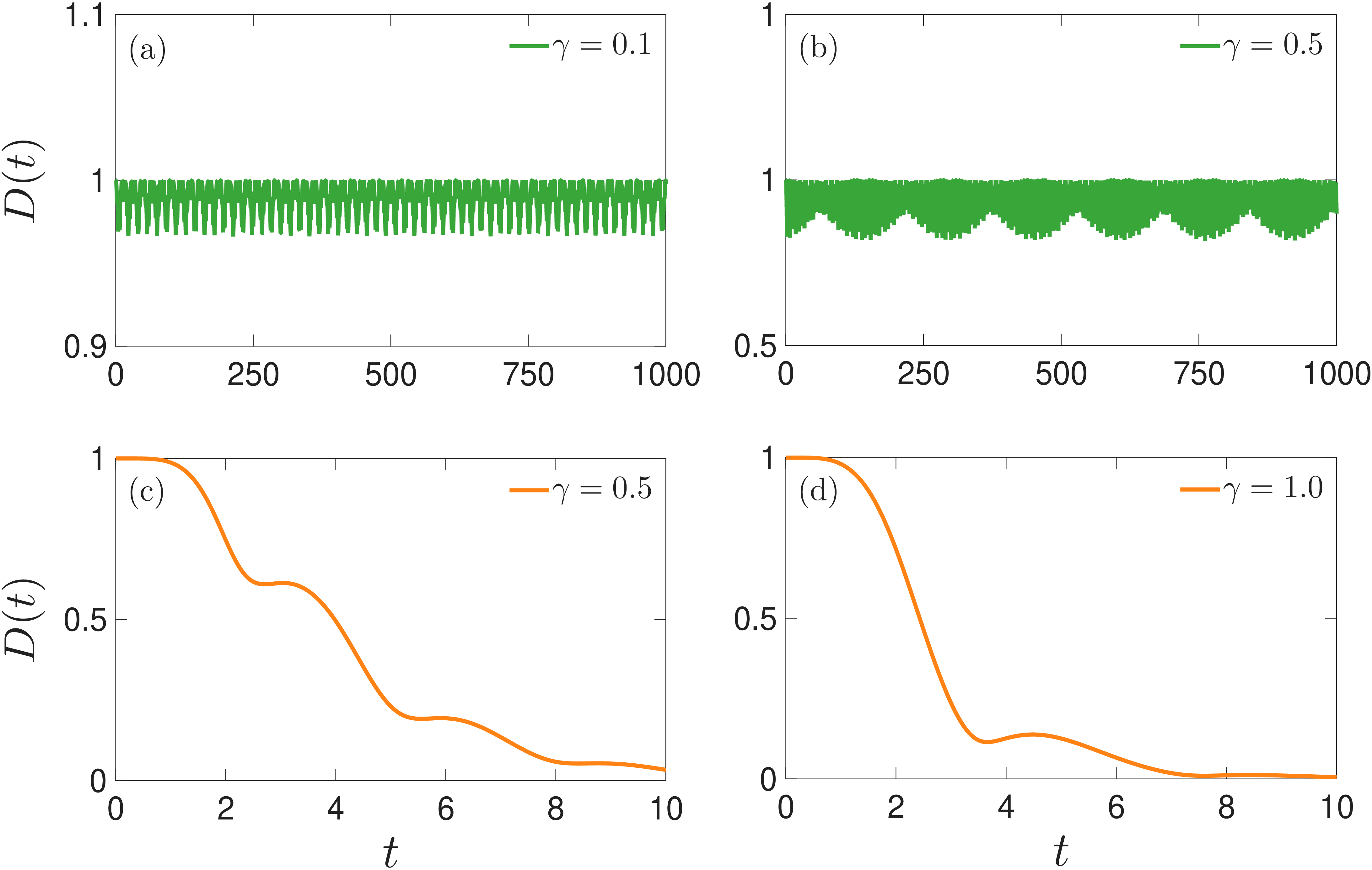
Figure 2 illustrate a set of dynamical results for the trace distance in both the \(\mathcal{PT}\)-unbroken phase (upper panel) and the symmetry broken phase (lower panel). As can be seen, the trace distance perfectly inherits the dynamical trends of the density matrix. In the \(\mathcal{PT}\)-unbroken phase [Figs. 2 (a) and (b)], \(D(t)\) exhibits persistent oscillations. In the broken phase [Figs. 2 (c) and (d)], it shows damped oscillations. We have numerically checked the dynamical trends in these two phases are independent of the initial states.
![Figure 3: Time evolution of the trace distance D(t) in the \mathcal{APT}-unbroken phase with \gamma=1.5 under different initial state pairs. Upper row [(a), (b)]: Initial states are \hat{\rho}_1(0)=|S_1\rangle\langle S_1| and \hat{\rho}_2(0)=|S_3\rangle\langle S_3|. Middle row [(c), (d)]: Initial states are \hat{\rho}_1(0)=|S_1\rangle\langle S_1| and \hat{\rho}_2(0)=|S_2\rangle\langle S_2|. Lower row [(e), (f)]: Initial states are \hat{\rho}_1(0)=|S_1\rangle\langle S_1| and \hat{\rho}_2(0)=0.5|S_1\rangle\langle S_1| + 0.5|S_2\rangle\langle S_2|. Left panel: \eta_1 = 0.5, \eta_2 = 1. Right panel: \eta_1 = 1, \eta_2 = 0.5.](/article/2606.24185/A23.png "fig:")
Interestingly, the dynamical trends of the trace distance in the \(\mathcal{APT}\)-unbroken phase exhibit rich decaying patterns that depend on the initial states. Representative results are shown in Figs. 3 for three initial state pairs. From Figs. 3 (a) and (b), we observe that under the initial pure state pair \(\hat{\rho}_1(0)=|S_1\rangle\langle S_1|\) and \(\hat{\rho}_2(0)=|S_3\rangle\langle S_3|\), the trace distance follows a monotonic exponential decay dominated by the leading-order term \(e^{-\Delta \Gamma t}\). In contrast, for the different initial pure state pair \(\hat{\rho}_1(0)=|S_1\rangle\langle S_1|\) and \(\hat{\rho}_2(0)=|S_2\rangle\langle S_2|\), shown in Figs. 3 (c) and (d), the trace distance exhibits a distinct non-monotonic evolution characterized by a prominent “bump" or”dip" before eventually decaying to zero. For comparison, we also consider an initial state pair that contains mixed initial state: \(\hat{\rho}_1(0)=|S_1\rangle\langle S_1|\) and \(\hat{\rho}_2(0)=0.5|S_1\rangle\langle S_1|+0.5|S_2\rangle\langle S_2|\), as shown in Figs. 3 (e) and 3 (f). In this case, the trace distance drops rapidly at very short times, followed by a transient plateau before entering the asymptotic decaying regime.
The rich decaying patterns arise from the structural inequivalence between sites in the non-Hermitian SSH lattice model due to alternating gain and loss, as well as from the initial-state-dependent superpositions of exponential decaying terms inherent in Eq. (6 ), since different initial states yield different expansion coefficients. In the early stages of evolution, the rapidly decaying modes have not yet subsided. The superposition of these rapidly decaying modes, with their differing coefficients, can induce a transient overshoot or a plateau-like structure, depending on the specific combination of exponential terms \(e^{(\Gamma_m+\Gamma_n)t}\). Only after these fast-decaying transient terms fully die out does the system enter the asymptotic regime, governed solely by the slowest decay rate, which restores the standard monotonic exponential decay. A detailed analysis is presented in Appendix 7.
These rich decaying patterns indicate that, while the long-time relaxation is universally dictated by the gap \(\Delta \Gamma\), the transient short-time information dynamics in non-Hermitian SSH lattice models are highly sensitive to the spatial configuration of the initial states. These intrinsic closed-system features provide an essential baseline for our subsequent investigation of pure dephasing effects.
3 Dynamical response to pure dephasing↩︎
In this section, we turn to the effects of dephasing on the dynamical evolution of the trace distance in the model described by Eq. (1 ). Through both analytical analysis and extensive numerical simulations, we reveal initial-state-dependent dephasing effects: depending on the initial excitation site, increasing dephasing can either accelerate decay or stabilize the trace distance.
3.1 Quantum master equation↩︎
To describe additional dephasing effects on non-Hermitian systems, we consider quantum master equation that describes the dynamical evolution of normalized density matrix \(\hat{\rho}(t)\) [75], [83], [84] \[\begin{gather} \frac{d}{dt}\hat{\rho}(t) = -i[\hat{H}\hat{\rho}(t) - \hat{\rho}(t)\hat{H}^{\dagger}] + \sum_k\mathcal{D}_k[\hat{\rho}(t)]\\ - i\mathrm{Tr}[\hat{\rho}(t)(\hat{H}^{\dagger} - \hat{H})]\hat{\rho}(t), \label{eq:master} \end{gather}\tag{7}\] where \(\hat{H}\) is the non-Hermitian Hamiltonian defined in Eq. 2 . The term \(\mathcal{D}_k[\hat{\rho}] = \gamma_k\left(\hat{L}_k\hat{\rho}\hat{L}_k^\dagger - \frac{1}{2}\{\hat{L}_k^\dagger\hat{L}_k,\hat{\rho}\}\right)\) represents the Lindblad dissipator capturing the external dissipation, where \(\hat{L}_k\) and \(\gamma_k\) denote the \(k\)-th jump operator and its corresponding decay rate, respectively. The last term on the right-hand-side of Eq. (7 ) denotes a correction term that ensures the conservation of probability [86]. In our model, we specifically focus on the effect of local pure dephasing, characterized by a uniform pure dephasing strength \(\gamma_d\) across all sites (i.e., we set \(\gamma_k = \gamma_d\) for all \(k\)) and local jump operators \(\hat{L}_k = |{S_k}\rangle\langle {S_k}|\) (\(k \in \{1,2,3,4\}\)) in the single-excitation subspace.
The formal solution of Eq. 7 can be expressed as [75] \[\hat{\rho}(t) = \frac{\operatorname{vec}^{-1}\!\left[ e^{\mathcal{L}_0 t} \operatorname{vec}[\hat{\rho}(0)] \right]}{\operatorname{Tr}\!\left( \operatorname{vec}^{-1}\!\left[ e^{\mathcal{L}_0 t} \operatorname{vec}[\hat{\rho}(0)] \right] \right)},\label{xingshi}\tag{8}\] where \(\operatorname{vec}(\mathcal{O})\) transforms an operator \(\mathcal{O}\) into a column vector, while \(\operatorname{vec}^{-1}\) is its inverse operation that converts a column vector back into matrix form. The Liouvillian superoperator \(\mathcal{L}_0\) is defined by \(\mathcal{L}_0[\hat{\rho}] = -i[\hat{H}\hat{\rho} - \hat{\rho}\hat{H}^{\dagger}] + \sum_k\mathcal{D}_k[\hat{\rho}]\), and \(e^{\mathcal{L}_0t}\) denotes its matrix exponential. The relaxation dynamics of the system are fundamentally governed by the eigenvalues of \(\mathcal{L}_0\), denoted as \(\{\mu_j = \mathcal{E}_j + i\alpha_j\}\). Sorting these eigenvalues so that their real parts are in descending order, \(\mathcal{E}_1 \geq \mathcal{E}_2 \geq \dots\), the long-time relaxation toward the steady state is determined by the Liouvillian gap, \(\Delta\mathcal{E} = \mathcal{E}_1 - \mathcal{E}_2\). Consequently, the characteristic relaxation time is given by \(\tau_o = 1/|\Delta\mathcal{E}|\) [75].
3.2 Initial-state dependent dephasing effects: Analytical treatment and numerical results↩︎
In this subsection, we combine simplified analytical treatments with complete numerical simulations based on Eq. 7 to reveal the intricate effects of dephasing. In particular, we show both analytically and numerically that the initial state plays a major role in shaping these dephasing effects. For the same set of initial states, systems in different phases exhibit similar dynamical trends upon increasing the dephasing strength. We focus on the dynamical evolution of the trace distance here, but our analysis applies to other state-based information-theoretic quantities.
3.2.1 Equation of motion in the strong dephasing limit↩︎
While the quantum master equation introduced in Eq. 7 provides a formally complete description of the system’s dynamics in the presence of pure dephasing, its highly nonlinear structure and the intricate coupling between populations (diagonal elements) and coherences (off-diagonal elements) present significant challenges for obtaining direct analytical insights. To resolve the underlying physical mechanisms and to systematically understand how dephasing competes with non-Hermiticity, it is instructive to first examine the limiting regime of strong pure dephasing with \(\gamma_d \to \infty\). In this limit, the rapid decay of quantum coherences allows us to decouple the fast and slow degrees of freedom, simplifying the full master equation into a set of effective, classically behaved rate equations for the diagonal elements. This simplification provides a tractable analytical framework to investigate initial-state-dependent dephasing effects that manifest in the strong-dephasing limit and enables us to elucidate the origin of this initial-state dependence.
Specifically, in the strong dephasing limit, the dephasing rate \(\gamma_d\) constitutes the dominant energy scale, significantly exceeding both the hopping parameters \(|\eta_1|, |\eta_2|\) and the non-Hermitian strength \(|\gamma|\). In this regime, the off-diagonal elements \(\rho_{nm}(t)=\langle n|\hat{\rho}(t)|m\rangle\;(n\neq m)\) decay rapidly to zero on a extremely short timescale; For notational simplicity, we will use the shorthand \(|n\rangle \equiv |S_n\rangle\) throughout this subsection. Consequently, the system’s density matrix can be effectively approximated by a purely diagonal form \[\hat{\rho}(t) \simeq \operatorname{diag}(\rho_{11}(t), \rho_{22}(t), \rho_{33}(t), \rho_{44}(t)). \label{eq:diagonal95approx}\tag{9}\] Here, \(\rho_{nn}(t)=\langle n|\hat{\rho}(t)| n\rangle\) (\(n=1,2,3,4\)). \(\operatorname{diag}(\cdot)\) denotes a diagonal matrix. Under this approximation, the contributions of the off-diagonal elements to the master equation emerge as higher-order infinitesimals and can be safely neglected. Thus, understanding the dynamical evolution is reduced to solving the equations of motion solely for the diagonal populations. For simplicity, the time dependence is suppressed hereafter.
Strictly speaking, the exact time evolution of the diagonal element \(\rho_{nn}\) is obtained by projecting Eq. 7 onto the local basis \[\begin{align} \frac{d}{dt}\rho_{nn} &= \underbrace{-i\langle n|[\hat{H}\hat{\rho} - \hat{\rho}\hat{H}^{\dagger}]|n\rangle}_{A_n} \\ &\quad + \underbrace{\langle n|\sum_k\mathcal{D}_k[\hat{\rho}]|n\rangle}_{B_n} \\ &\quad \underbrace{- i\operatorname{Tr}\left[\hat{\rho}(\hat{H}^{\dagger} - \hat{H})\right]\rho_{nn}}_{C_n}. \end{align} \label{eq:diag95evolution}\tag{10}\] To obtain the correct equations of motion for the diagonal populations in the strong-dephasing limit, we examine the three terms \(A_n\), \(B_n\) and \(C_n\) in turn.
We first focus on the term \(A_n\). We expand it by inserting a complete set of states \(\sum_m |m\rangle\langle m| = \mathrm{I}\), \[A_n = -i \sum_m \left( H_{nm}\rho_{mn} - \rho_{nm}H_{mn}^* \right).\] Since the Hamiltonian \(\hat{H}\) contains Hermitian hopping and non-Hermitian on-site terms, its matrix elements satisfy \(H_{nm}=H_{mn}\) for \(n \neq m\), and \(H_{nn} = i\gamma_n\) (We have \(\gamma_{1,3}=-\gamma_{2,4}=\gamma\)). Separating the \(m=n\) term from the summation yields \[\begin{align} A_n &=& -i \left( i\gamma_n \rho_{nn} - \rho_{nn}(-i\gamma_n) \right) - i \sum_{m \neq n} H_{nm}(\rho_{mn} - \rho_{nm})\nonumber \\ &=& 2\gamma_n \rho_{nn} - i \sum_{m \neq n} H_{nm}(\rho_{mn} - \rho_{nm}).\label{eq:An95expanded} \end{align}\tag{11}\] To evaluate the remaining summation, we must examine the off-diagonal elements \(\rho_{nm}\) (\(n \neq m\)). The evolution of the off-diagonal elements is governed by \[\label{eq:144} \begin{align} \frac{d}{dt}\rho_{nm} =& -i \sum_m (H_{nm}\rho_{mm} - \rho_{nm}H_{mm}^*) \\ & - i\operatorname{Tr}\bigl[\hat{\rho}(\hat{H}^{\dagger} - \hat{H})\bigr]\rho_{nm} \\ & - \gamma_d \rho_{nm}. \end{align}\tag{12}\] In the strong dephasing limit of \(\gamma_d \to \infty\), the off-diagonal elements almost instantaneously reach their stationary values with \(\frac{d}{dt}\rho_{nm} \simeq 0\). Neglecting higher-order terms and retaining only the dominant populations in Eq. (12 ), we obtain \[0 \simeq -i H_{nm}(\rho_{mm} - \rho_{nn}) - \gamma_d \rho_{nm}.\] We thus obtain \(\rho_{nm} \simeq -i \frac{H_{nm}}{\gamma_d} (\rho_{mm} - \rho_{nn})\). Inserting this expression back into the sum in Eq. 11 , we have \[\begin{align} -i H_{nm}(\rho_{mn} - \rho_{nm}) &=& -i H_{nm} \biggl[ -i \frac{H_{mn}}{\gamma_d}(\rho_{nn} - \rho_{mm}) \nonumber\\ && - \biggl( -i \frac{H_{nm}}{\gamma_d}(\rho_{mm} - \rho_{nn}) \biggr) \biggr] \nonumber\\ &=& -i H_{nm} \biggl[ -2i \frac{H_{nm}}{\gamma_d}(\rho_{nn} - \rho_{mm}) \biggr] \nonumber\\ &=& \frac{2 H_{nm}^2}{\gamma_d} (\rho_{mm} - \rho_{nn}). \end{align}\] Thus, the term \(A_n\) is evaluated as \[A_n = 2\gamma_n \rho_{nn} + \sum_{m \neq n} \frac{2 H_{nm}^2}{\gamma_d} (\rho_{mm} - \rho_{nn}). \label{eq:An952}\tag{13}\]
We then turn to the terms \(B_n\) and \(C_n\). For the local pure dephasing with \(\hat{L}_n = |n\rangle\langle n|\), the projected dissipator reads \[\begin{align} \langle n|\mathcal{D}_n[\hat{\rho}]|n\rangle &=& \gamma_d \Big(\langle n|n\rangle\langle n|\hat{\rho}|n\rangle\langle n|n\rangle \nonumber\\ &&-\frac{1}{2}\langle n|\{|n\rangle\langle n|, \hat{\rho}\}|n\rangle \Big)=0. \label{eq:Bn951} \end{align}\tag{14}\] We thus infer that \(B_n = 0\). This confirms that pure dephasing does not induce population transfer between sites. Lastly, to evaluate \(C_n\), we first note that \(S \equiv \operatorname{Tr}\left[\hat{\rho}(\hat{H}^{\dagger} - \hat{H})\right]=\sum_m \rho_{mm} (H_{mm}^* - H_{mm}) = -2i\sum_m \rho_{mm} \operatorname{Im}(H_{mm})\). Since \(\operatorname{Im}(H_{mm}) = \gamma_m\), we can rewrite \(S\) as \[S = -2i\gamma(\rho_{11} - \rho_{22} + \rho_{33} - \rho_{44}) \equiv -2i\gamma M, \label{eq:S952}\tag{15}\] where we have introduced the population imbalance parameter \(M = \rho_{11} - \rho_{22} + \rho_{33} - \rho_{44}\). Consequently, the correction term is formulated as \[C_n = -i S \rho_{nn} = -2\gamma M \rho_{nn}. \label{eq:Cn}\tag{16}\]
By substituting Eqs. 13 and 16 into Eq. 10 and noting \(B_n=0\), we obtain the simplified equation of motion for the population element \(\rho_{nn}\) in the strong dephasing limit, \[\frac{d}{dt}\rho_{nn} = 2\gamma_n \rho_{nn} + \sum_{m \neq n} \frac{2 H_{nm}^2}{\gamma_d} (\rho_{mm} - \rho_{nn}) - 2\gamma M \rho_{nn}. \label{eq:complete95diag}\tag{17}\] This equation of motion keeps the leading order term in \(1/\gamma_d\). Defining the effective hopping rates \(\kappa_1 = 2\eta_1^2/\gamma_d\) and \(\kappa_2 = 2\eta_2^2/\gamma_d\), we obtain the complete set of coupled equations of motion for the four diagonal elements \[\begin{align} \dot{\rho}_{11} &= 2\gamma\rho_{11}(1 - M) + \kappa_1(\rho_{22} - \rho_{11}), \tag{18} \\[2pt] \begin{aligned} \dot{\rho}_{22} &= -2\gamma\rho_{22}(1 + M) + \kappa_1(\rho_{11} - \rho_{22}) \\ &\quad + \kappa_2(\rho_{33} - \rho_{22}), \end{aligned} \tag{19} \\[2pt] \begin{align} \dot{\rho}_{33} &= 2\gamma\rho_{33}(1 - M) + \kappa_2(\rho_{22} - \rho_{33}) \\ &\quad + \kappa_1(\rho_{44} - \rho_{33}), \end{align} \tag{20} \\[2pt] \dot{\rho}_{44} &= -2\gamma\rho_{44}(1 + M) + \kappa_1(\rho_{33} - \rho_{44}). \tag{21} \end{align}\]
In the strong-dephasing regime, the effective dynamics described by Eqs. 18 21 acquire a clear physical interpretation in terms of population flow between sites with alternating gain and loss. The terms on the right-hand-side of Eqs. 18 –21 that are proportional to the non-Hermiticity strength \(\gamma\) generate a pronounced local distinction: the local populations at gain sites are amplified, while those at loss sites experience suppression. Consequently, the long-time relaxation becomes highly sensitive to the initial state configuration. The remaining terms on the right-hand-side of Eqs. 18 21 , which are induced by dephasing, tend to suppress spatial transport of population between sites, since the effective hopping rates \(\kappa_1 = 2\eta_1^2/\gamma_d\) and \(\kappa_2 = 2\eta_2^2/\gamma_d\) scale inversely with the dephasing strength.
This set of equations [Eqs. 18 –21 ] serves as the theoretical basis for our subsequent identification of initial-state-dependent dephasing effects. That being said, the highly nonlinear nature of these equations–arising from the population imbalance parameter \(M\) that originates from the correction term \(C_n\)–implies a strong sensitivity to initial conditions and presents a challenge for direct analytical treatment. To circumvent this nonlinearity, we draw inspiration from the formal solution of the master equation in Eq. (8 ), where the correction term manifests as the normalization factor in the denominator. Analogously, we introduce a set of unnormalized populations \(x_n\) such that the physical populations are subsequently recovered via instantaneous normalization \[\rho_{nn} = \frac{x_n}{\sum_{k=1}^4 x_k}. \label{eq:normalization95x}\tag{22}\] By factoring out the correction terms (i.e., the \(-2\gamma M\rho_{nn}\) terms in Eqs. 18 –21 ), the unnormalized populations \(\{x_n\}\) obey a purely linear set of rate equations \[\begin{align} \dot{x}_1 &= 2\gamma x_1 + \kappa_1(x_2 - x_1), \tag{23} \\ \dot{x}_2 &= -2\gamma x_2 + \kappa_1(x_1 - x_2) + \kappa_2(x_3 - x_2), \tag{24} \\ \dot{x}_3 &= 2\gamma x_3 + \kappa_2(x_2 - x_3) + \kappa_1(x_4 - x_3), \tag{25} \\ \dot{x}_4 &= -2\gamma x_4 + \kappa_1(x_3 - x_4). \tag{26} \end{align}\] We have numerically verified that Eqs. (23 )-(26 ) yield exactly the same population results at any time as Eqs. 18 –21 upon normalization according to Eq. (22 ).
The linearized equations of motion in Eqs. (23 )-(26 ) allow us to clearly isolate the competition between non-Hermiticity-induced local amplification/decay and dephasing-induced spatial diffusion in the strong-dephasing limit, with the latter can be regarded as perturbations since \(\gamma \gg \kappa_{1,2}\). In the following, we elucidate the initial-state-dependent dephasing effects by examining the dynamics of the trace distance \(D(t)\) under different initial-state configurations using this linearized approach.
3.2.2 Case I: Accelerating decay↩︎
We first demonstrate that dephasing can accelerate the decay of the trace distance, thus playing a detrimental role as in Hermitian systems. We showcase this phenomenon by harnessing the fact that local population at the gain site gets amplified while strong dephasing suppresses the spatial transport of population. Specifically, we consider two initial states: a pure state \(\hat{\rho}_1(0) = |S_1\rangle\langle S_1|\), which is initialized at the first gain site, and a mixed state \(\hat{\rho}_2(0) = \frac{1}{2}|S_1\rangle\langle S_1| + \frac{1}{2}|S_2\rangle\langle S_2|\), which evenly distributes initial population between the adjacent gain and loss sites. In the following, we use superscripts \((1)\) and \((2)\) to denote population dynamics from initial states \(\hat{\rho}_1(0)\) and \(\hat{\rho}_2(0)\), respectively.
For the initial pure state \(\hat{\rho}_1(0)\), the unnormalized population is initialized at the first gain site with \(x_1^{(1)}(0) = 1\). In the strong-dephasing limit, we have \(\gamma \gg \kappa_{1,2}\), the unnormalized population \(x_1^{(1)}(t)\) at finite times experiences an exponential amplification, \(x_1^{(1)}(t) \simeq e^{2\gamma t}\). Upon normalization Eq. 22 , the physical state remains locked at its initial configuration, \(\hat{\rho}_1(t) \simeq \operatorname{diag}(1,0,0,0)\).
As for the initial mixed state \(\hat{\rho}_2(0)\), the unnormalized populations are initialized as \(x_1^{(2)}(0) = 0.5\) and \(x_2^{(2)}(0) = 0.5\), while \(x_3^{(2)}(0) = x_4^{(2)}(0) = 0\). Governed overwhelmingly by the non-Hermitian terms (\(\gamma \gg \kappa_{1,2}\)), Eqs. (23 ) and (24 ) indicate that the initial unnormalized populations at the first two sites approximately evolve as \[x_1^{(2)}(t) \simeq 0.5 e^{2\gamma t}, \qquad x_2^{(2)}(t) \simeq 0.5 e^{-2\gamma t}.\] To justify the omission of the effective hopping terms in evaluating the physical state, we explicitly calculate the probability leakage to the third site, which is initially unoccupied. Noting that the population \(x_3^{(2)}(t)\) at finite times is continuously driven by leakage from the second site, we substitute \(x_2^{(2)}(t)\) into Eq. 25 and obtain a first-order inhomogeneous differential equation \[\dot{x}_3^{(2)} \simeq 2\gamma x_3^{(2)} + \kappa_2 \left(0.5 e^{-2\gamma t}\right).\] Solving this equation with the integrating factor \(e^{-2\gamma t}\) and the initial condition \(x_3^{(2)}(0) = 0\) yields \[x_3^{(2)}(t) \simeq \frac{\kappa_2}{8\gamma} \left( e^{2\gamma t} - e^{-2\gamma t} \right).\] In the strong-dephasing regime where \(\gamma \gg \kappa_{1,2}\), the factor \(\kappa_2/\gamma\) acts as a higher-order infinitesimal. This leads to a vanishing physical population: \(\rho_{33}^{(2)}(t) \sim \mathcal{O}(\kappa_2/\gamma) \to 0\). An analogous sequential suppression applies to the fourth site, yielding \(\rho_{44}^{(2)}(t) \sim \mathcal{O}(\kappa_1 \kappa_2 / \gamma^2) \to 0\). Therefore, the normalized physical state \(\hat{\rho}_2(t)\) is determined almost entirely by the competition between the primary local gain and loss at the first two sites: \(\hat{\rho}_2(t) \simeq \operatorname{diag}(\rho_{11}^{(2)}(t), \rho_{22}^{(2)}(t), 0, 0)\), where \[\begin{align} \rho_{11}^{(2)}(t) &\simeq \frac{x_1^{(2)}(t)}{x_1^{(2)}(t) + x_2^{(2)}(t)} = \frac{e^{4\gamma t}}{1 + e^{4\gamma t}}, \tag{27} \\[6pt] \rho_{22}^{(2)}(t) &\simeq \frac{x_2^{(2)}(t)}{x_1^{(2)}(t) + x_2^{(2)}(t)} = \frac{1}{1 + e^{4\gamma t}}. \tag{28} \end{align}\] As can be seen, \(\hat{\rho}_2(t)\) approaches \(\hat{\rho}_1(t)\) exponentially in time.
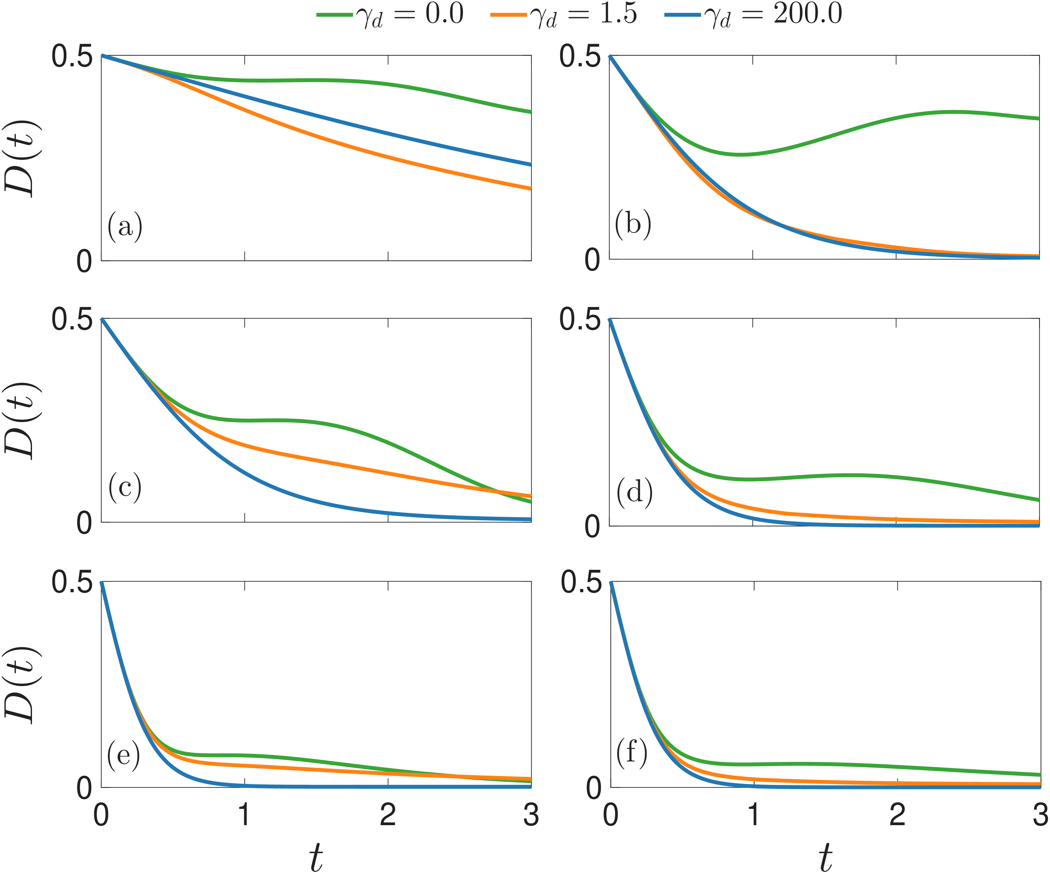
This exponential approach of the states directly implies an exponential decay of the trace distance in the strong-dephasing limit: \[\begin{align} D(t) &= \frac{1}{2} \left( \left|1 - \frac{e^{4\gamma t}}{1+e^{4\gamma t}}\right| + \left|0 - \frac{1}{1+e^{4\gamma t}}\right| \right) \\ &= \frac{1}{1+e^{4\gamma t}}. \end{align}\] Thus, the trace distance decays exponentially from \(0.5\) toward \(0\). To verify this theoretical prediction, we present a set of dynamical results for the trace distance in Fig. 4 obtained by solving Eq. (7 ) for the initial states \(\hat{\rho}_1(0) = |S_1\rangle\langle S_1|\) and \(\hat{\rho}_2(0) = \frac{1}{2}|S_1\rangle\langle S_1| + \frac{1}{2}|S_2\rangle\langle S_2|\). Upon increasing the dephasing strength, we indeed observe an exponentially accelerated decay of the trace distance in all three phases.
3.2.3 Case II: Partial stabilization↩︎
We next show that increasing the dephasing strength does not always lead to accelerated decay of the trace distance toward zero, but can instead stabilize it to a finite value smaller than the initial value in the long-time limit under strong dephasing. To illustrate this partial stabilization phenomenon, we consider two pure initial states: \(\hat{\rho}_1(0) = |S_1\rangle\langle S_1|\) and \(\hat{\rho}_2(0) = |S_2\rangle\langle S_2|\), which are initialized at adjacent gain and loss sites, respectively.
For the initial state \(\hat{\rho}_1(0)\), we previously showed that \(\hat{\rho}_1(t) \simeq \operatorname{diag}(1,0,0,0)\). We therefore only need to analyze the dynamics starting from the initial state \(\hat{\rho}_2(0) = |S_2\rangle\langle S_2|\), which implies that \(x_2^{(2)}(0) = 1\) and all other unnormalized populations vanish. According to Eq. 24 , its unnormalized population \(x_2^{(2)}(t)\) in the strong-dephasing limit approximately evolves as \[x_2^{(2)}(t) \simeq e^{-2\gamma t}.\] Crucially, the second site is coupled to two adjacent gain sites. Although the unnormalized populations \(x_1^{(2)}\) and \(x_3^{(2)}\) are initially zero, they become nonzero at later times due to leakage from \(x_2^{(2)}\). Substituting \(x_2^{(2)}(t) \simeq e^{-2\gamma t}\) into Eqs. 23 and 25 , and neglecting the infinitesimal terms \(-\kappa_1 x_1\) and \(-(\kappa_1+\kappa_2) x_3\) (since \(2\gamma \gg \kappa_{1,2}\)), the linear equations for these adjacent gain sites simplify to first-order differential equations: \[\begin{align} \dot{x}_1^{(2)} &\simeq 2\gamma x_1^{(2)} + \kappa_1 e^{-2\gamma t}, \\ \dot{x}_3^{(2)} &\simeq 2\gamma x_3^{(2)} + \kappa_2 e^{-2\gamma t}. \end{align}\] With the initial conditions \(x_1^{(2)}(0) = x_3^{(2)}(0) = 0\), we obtain the following approximate solutions: \[x_1^{(2)}(t) \simeq \frac{\kappa_1}{4\gamma} \left(e^{2\gamma t} - e^{-2\gamma t}\right) \simeq \left.\frac{\kappa_1}{4\gamma} e^{2\gamma t}\right|_{t\to\infty},\] \[x_3^{(2)}(t) \simeq \frac{\kappa_2}{4\gamma} \left(e^{2\gamma t} - e^{-2\gamma t}\right) \simeq \left.\frac{\kappa_2}{4\gamma} e^{2\gamma t}\right|_{t\to\infty}.\]
Upon normalization \(\rho_{nn} = x_n / \sum_k x_k\), the identical exponential growth terms \(e^{2\gamma t}\) strictly cancel out. The system rapidly jumps into a stationary distribution which only has populations on the two gain sites \[\rho^{(2)}(t) \simeq \left( \frac{\kappa_1}{\kappa_1+\kappa_2}, 0, \frac{\kappa_2}{\kappa_1+\kappa_2}, 0 \right). \label{ab}\tag{29}\] Calculating the trace distance between \(\rho^{(1)}(t)\) and \(\rho^{(2)}(t)\) gives \[\begin{align} D(t \to \infty) &= \frac{1}{2} \sum_n \left|\rho_{nn}^{(1)}(t) - \rho_{nn}^{(2)}(t)\right| \\ &= \frac{\kappa_2}{\kappa_1+\kappa_2}<1. \end{align}\] The stationary value \(D(t \to \infty)\) is fully determined by \(\eta_{1,2}\) in the strong dephasing limit.
In Fig. 5, we present a set of numerical results for \(D(t)\) under varying dephasing strength obtained by solving Eq. (7 ) for the two initial states \(\hat{\rho}_1(0) = |S_1\rangle\langle S_1|\) and \(\hat{\rho}_2(0) = |S_2\rangle\langle S_2|\). From the figure, we observe that increasing the dephasing strength first accelerates the decay of the trace distance compared with the dynamics in the closed system, but ultimately stabilizes the trace distance to a finite value in the long-time limit. We verify that the numerical stationary value coincides exactly with our theoretical prediction \(\frac{\kappa_2}{\kappa_1+\kappa_2}\) in all three phases. Notably, once \(\eta_{1,2}\) are fixed, the stationary value of \(D(t)\) remains constant across different phases, as expected.
3.2.4 Case III: Complete stabilization↩︎
Interestingly, the previously discovered dephasing-induced stabilization can become complete in the sense that the evolution of the trace distance is entirely frozen, such that it remains at its initial value throughout the entire evolution. This complete stabilization can be illustrated by choosing the pure initial states \(\hat{\rho}_1(0) = |S_1\rangle\langle S_1|\) and \(\hat{\rho}_2(0) = |S_3\rangle\langle S_3|\), for which the system is initialized in two different gain sites.
As established, the initial state \(\hat{\rho}_1(0)\) yields \(\hat{\rho}_1(t) \simeq \operatorname{diag}(1,0,0,0)\) in the strong-dephasing limit. We now turn to the dynamics of \(\hat{\rho}_2(t)\) initialized at the third site, which is a gain site. The unnormalized population at this site grows as \(x_3^{(2)}(t) \simeq e^{2\gamma t}\). To obtain the detailed form of \(\hat{\rho}_2(t)\), we analyze the equations of motion for the nearby loss sites. Substituting \(x_3^{(2)}(t) \simeq e^{2\gamma t}\) into Eqs. 24 and 26 and neglecting the infinitesimal terms that do not involve \(x_3\) (since \(2\gamma \gg \kappa_{1,2}\)), we obtain \[\begin{align} \dot{x}_2^{(2)} &\simeq -2\gamma x_2^{(2)} + \kappa_2 e^{2\gamma t}, \\ \dot{x}_4^{(2)} &\simeq -2\gamma x_4^{(2)} + \kappa_1 e^{2\gamma t}. \end{align}\] Integrating these equations with zero initial populations yields \[x_2^{(2)}(t) \simeq \frac{\kappa_2}{4\gamma} e^{2\gamma t}, \qquad x_4^{(2)}(t) \simeq \frac{\kappa_1}{4\gamma} e^{2\gamma t}.\] Because the total population is dominated by the source term at the third gain site (\(\gamma \gg \kappa_{1,2}\)), the normalized populations at the loss sites are suppressed: \(\rho_{22} \sim \mathcal{O}(\kappa_2/\gamma)\) and \(\rho_{44} \sim \mathcal{O}(\kappa_1/\gamma)\). Consequently, the normalized density matrix remains localized at the third site: \[\hat{\rho}^{(2)}(t) \simeq \operatorname{diag}(0, 0, 1, 0).\] The corresponding trace distance at finite times then becomes \[D(t) \simeq \frac{1}{2}(|1-0| + |0-1|) = 1 = D(0).\] Thus, the dynamics of \(D(t)\) is completely frozen.
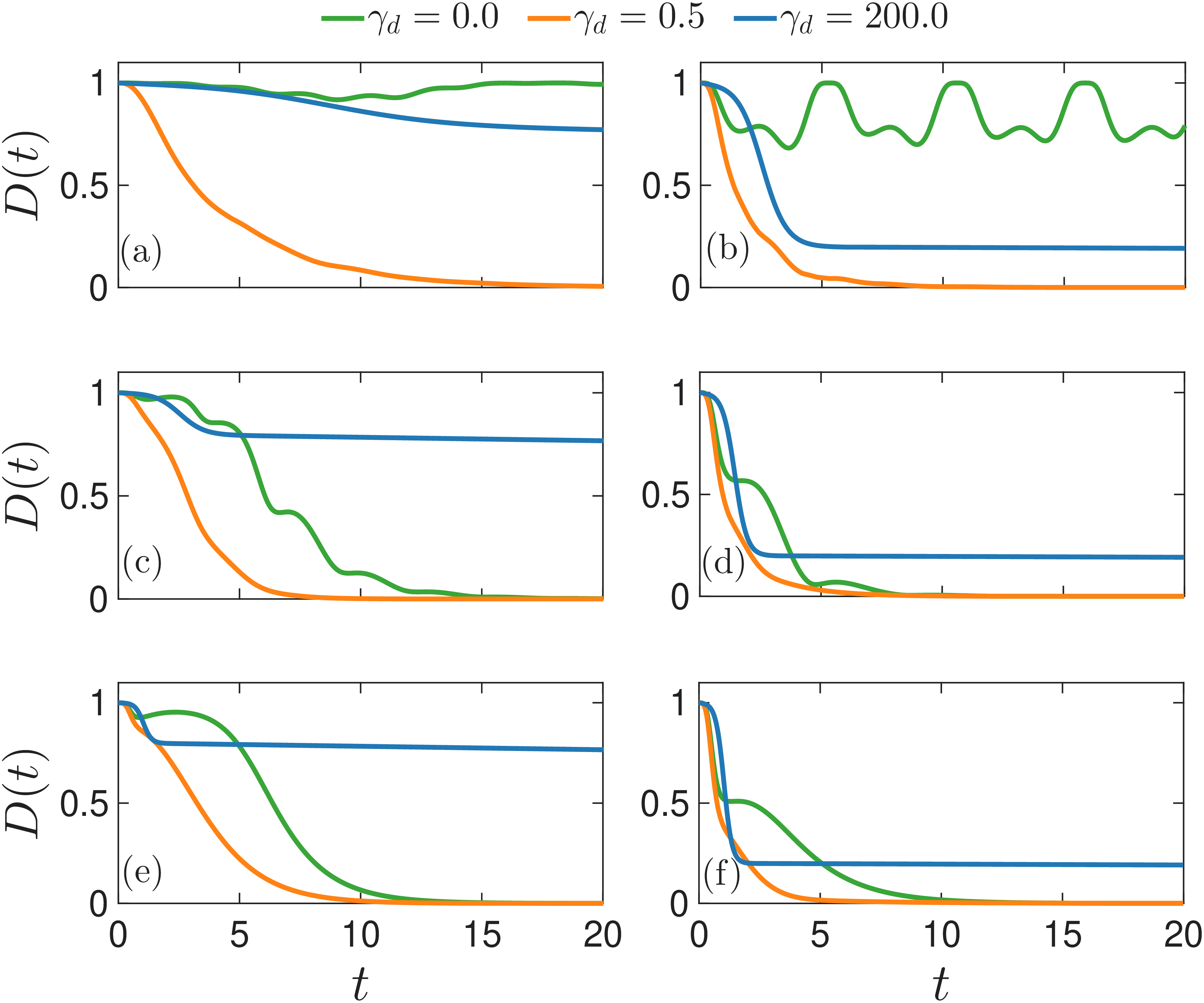
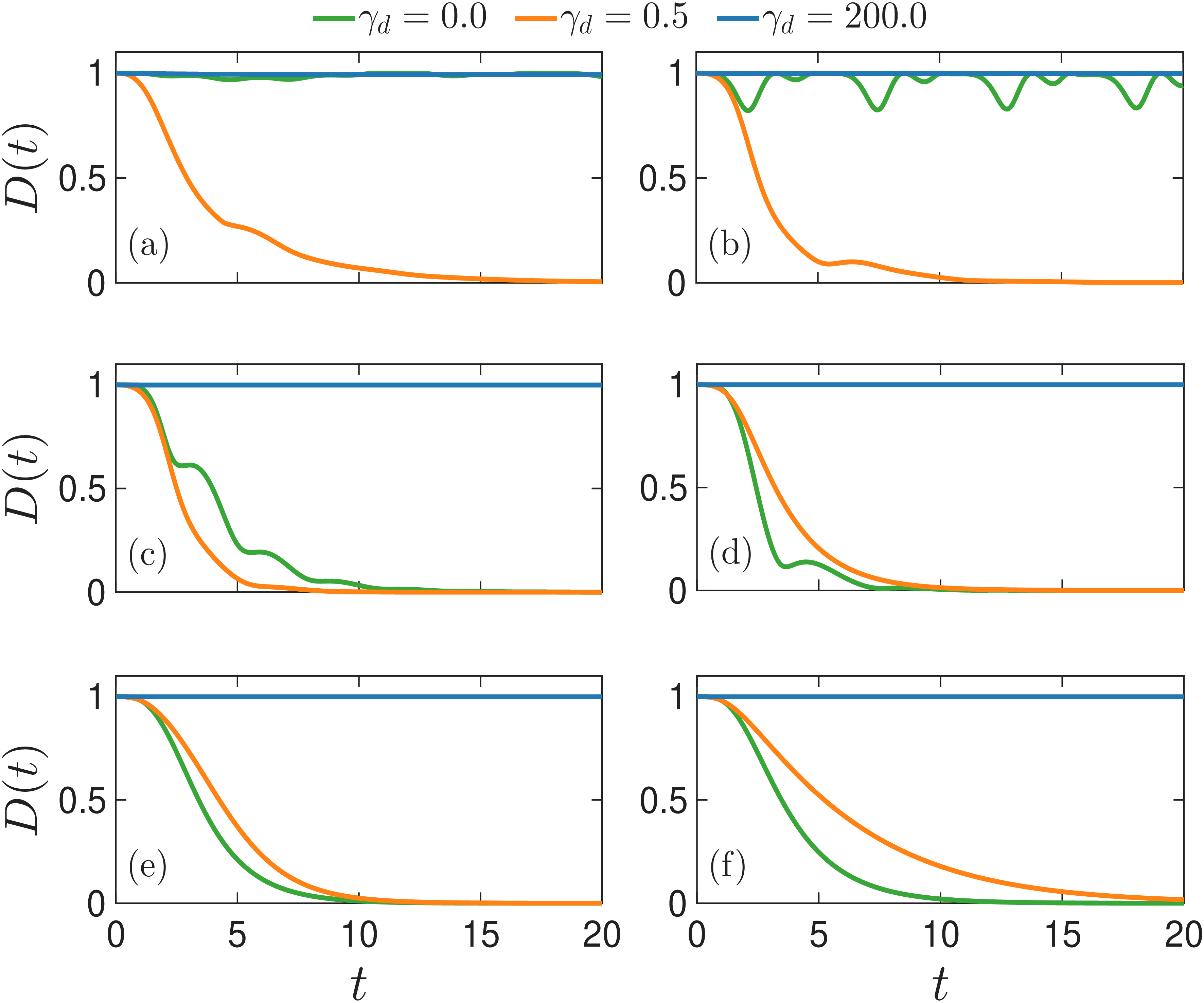
To confirm this theoretical expectation, in Fig. 6 we present a set of numerical results for the trace distance \(D(t)\) with varying dephasing strength \(\gamma_d\), obtained by solving Eq. (7 ) for the initial states \(\hat{\rho}_1(0) = |S_1\rangle\langle S_1|\) and \(\hat{\rho}_2(0) = |S_3\rangle\langle S_3|\). In both phases, we clearly see that the dynamics of \(D(t)\) is indeed completely suppressed in the strong-dephasing limit, thereby confirming our theoretical expectation. However, at small dephasing strengths, we identify a distinction between the \(\mathcal{PT}\)-unbroken and \(\mathcal{APT}\)-unbroken phases. In the former case, increasing the dephasing strength first transforms the persistent oscillations in the closed system into damped oscillations, thus playing a detrimental role. Only upon further increasing the dephasing strength does one observe a complete stabilization of the trace distance. In the latter case, by contrast, increasing the dephasing strength continuously suppresses the decay of the trace distance until complete stabilization is reached in the strong-dephasing limit, thereby marking an unconventional dephasing-induced continuous protection of information in the \(\mathcal{APT}\)-unbroken phase.
3.3 Dephasing-induced continuous protection in the \(\mathcal{APT}\) phase: Insight from Liouvillian gap↩︎
To gain further insight into the distinction between different phases at small dephasing strengths, as well as the dephasing-induced continuous protection in the \(\mathcal{APT}\) phase as showed in Fig. 6 (f), we turn to the spectrum of the Liouvillian superoperator \(\mathcal{L}_0\), from which we can extract the Liouvillian gap.
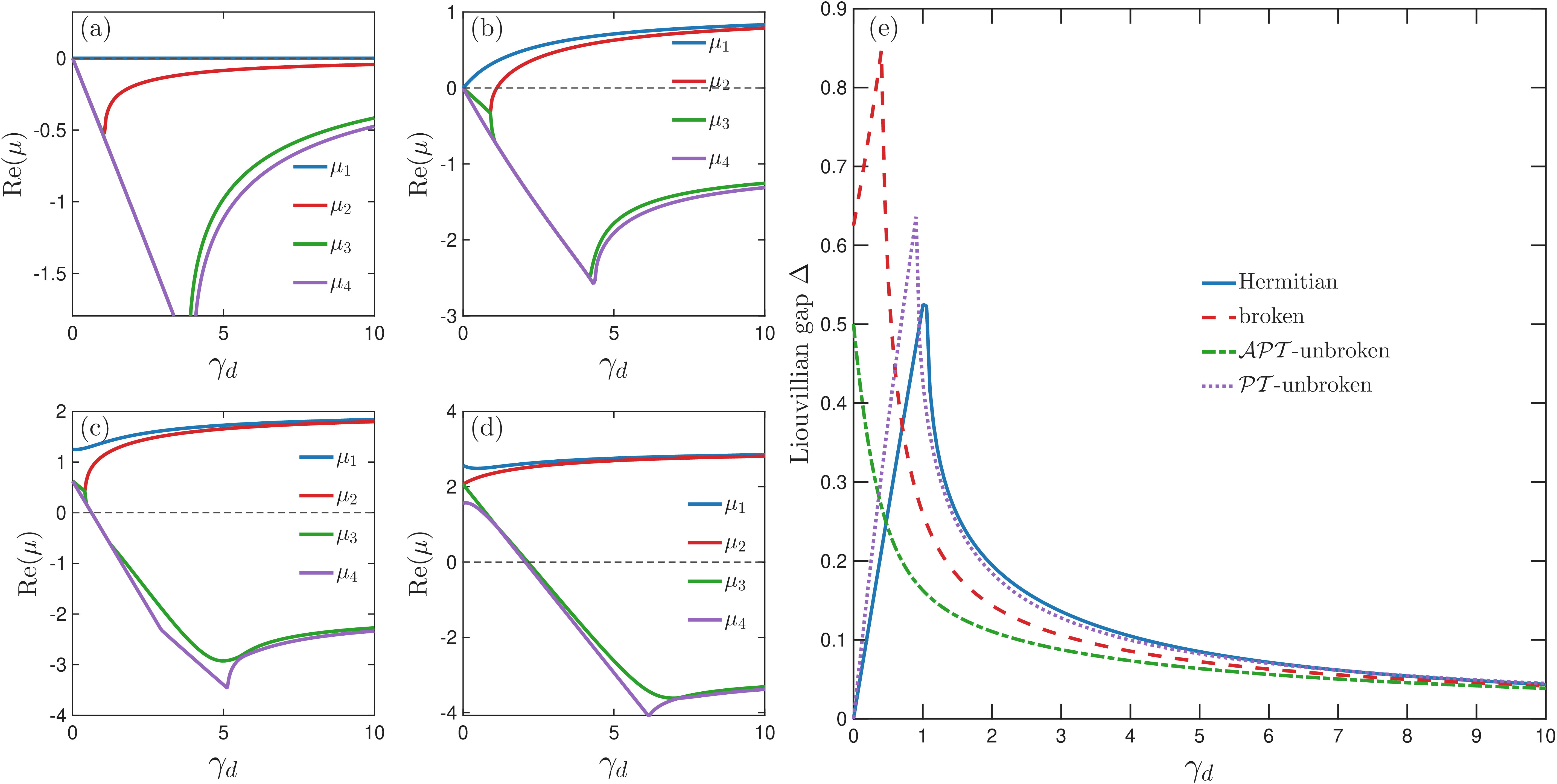
Figures 7 (a)-(d) illustrate the real parts of the ordered eigenvalues of \(\mathcal{L}_0\) as functions of the pure dephasing strength \(\gamma_d\) for the Hermitian system, the non-Hermitian system in the \(\mathcal{PT}\)-unbroken phase, the symmetry-broken phase, and the \(\mathcal{APT}\)-unbroken phase, respectively. From these four subplots, we extract the corresponding Liouvillian gap \(\Delta\mathcal{E} = \mathcal{E}_1 - \mathcal{E}_2\), which is summarized in Fig. 7 (e). A compelling observation from Fig. 7 (e) is that the behavior of the Liouvillian gap differs in the small-dephasing regime. In the Hermitian system and the non-Hermitian systems in the \(\mathcal{PT}\)-unbroken and symmetry-broken phases, the Liouvillian gap exhibits a nonmonotonic trend. In contrast, in the \(\mathcal{APT}\)-unbroken phase, the Liouvillian gap decreases monotonically with increasing \(\gamma_d\). This contrast explains why we observe a distinction between the \(\mathcal{APT}\) phase and the other two phases in Fig. 6 at small dephasing strengths, and why a continuous suppression of decay is observed only in the \(\mathcal{APT}\) phase. For a comprehensive understanding, we note that the monotonic behavior of the Liouvillian gap in the \(\mathcal{APT}\)-unbroken phase depends on the hopping parameters. For a different set of hopping parameters, e.g., \(\eta_1 = 0.5\) and \(\eta_2 = 1\) (distinct from those used in Figs. 6 and 7), a nonmonotonic trend of the Liouvillian gap can emerge in the \(\mathcal{APT}\)-unbroken phase. In Appendix 8, we present a detailed analysis of when a monotonic dependence of the Liouvillian gap on the dephasing strength can emerge in the \(\mathcal{APT}\)-unbroken phase.
Nevertheless, the non-Hermitian systems in all three phases share a universal asymptotic feature: in the strong-dephasing limit \(\gamma_d \to \infty\), the Liouvillian gaps collapse onto the same asymptotic curve and decay to zero, consistent with the complete dynamical freezing observed in Fig. 6. In Hermitian systems, such dynamical freezing in the strong-dephasing limit is typically interpreted as a quantum Zeno effect, since the impact of environmental dissipation can be interpreted as a continuous measurement on the system. Here, however, we do not interpret the dynamical freezing in non-Hermitian systems as a quantum Zeno effect, because the complete stabilization we observe occurs only for certain initial states, whereas the quantum Zeno effect is generally insensitive to the initial state and depends only on the measurement frequency (or, equivalently, the dissipation strength).
4 Multi-site system↩︎
To verify the scalability of the observed phenomena, we extend our analysis to a multi-site non-Hermitian SSH model constructed by regarding the previously addressed four-site system as the unit cell. For demonstration purposes, we consider a one-dimensional chain under open boundary conditions consisting of \(N = 10\) unit cells, amounting to a total of 40 sites. For each unit cell, we denote the corresponding annihilation operators as \(\hat{a}_j, \hat{b}_j, \hat{c}_j\), and \(\hat{d}_j\) for the \(j\)-th cell (\(j = 1, \dots, N\)). The total Hamiltonian is expressed as the sum of the Hermitian Su-Schrieffer-Heeger (SSH) part \(\hat{H}_0\) and the non-Hermitian term \(\hat{H}_\gamma\): \[\hat{H} = \hat{H}_0 + \hat{H}_\gamma,\] where \[\begin{align} \hat{H}_0 &= \sum_{j=1}^{N} \bigl( \eta_1 \hat{a}_j^\dagger \hat{b}_j + \eta_2 \hat{b}_j^\dagger \hat{c}_j + \eta_1 \hat{c}_j^\dagger \hat{d}_j + \rm{H.c.} \bigr) \nonumber \\ &\quad + \sum_{j=1}^{N-1} \bigl( \eta_2 \hat{d}_j^\dagger \hat{a}_{j+1} + \rm{H.c.} \bigr), \\ \hat{H}_{\gamma} &= i\gamma \sum_{j=1}^{N} \bigl( \hat{a}_j^\dagger \hat{a}_j - \hat{b}_j^\dagger \hat{b}_j + \hat{c}_j^\dagger \hat{c}_j - \hat{d}_j^\dagger \hat{d}_j \bigr). \end{align}\] Here, \(\eta_{1,2}\) remain the alternating inter-site coupling strengths, and \(\gamma\) quantifies the strength of the balanced gain and loss processes uniformly applied across the entire lattice.
Parallel to the treatment of the four-site model, we restrict our analysis to the single-excitation subspace. For this 40-site system, the subspace is spanned by the Fock states \(\{|S_1\rangle, |S_2\rangle, \dots, |S_{40}\rangle\}\), where \(|S_n\rangle\) represents a single excitation localized on the \(n\)-th site of the entire chain, with all other sites empty (e.g., \(|S_1\rangle = |100\dots0\rangle\), \(|S_2\rangle = |010\dots0\rangle\), up to \(|S_{40}\rangle = |000\dots1\rangle\)).
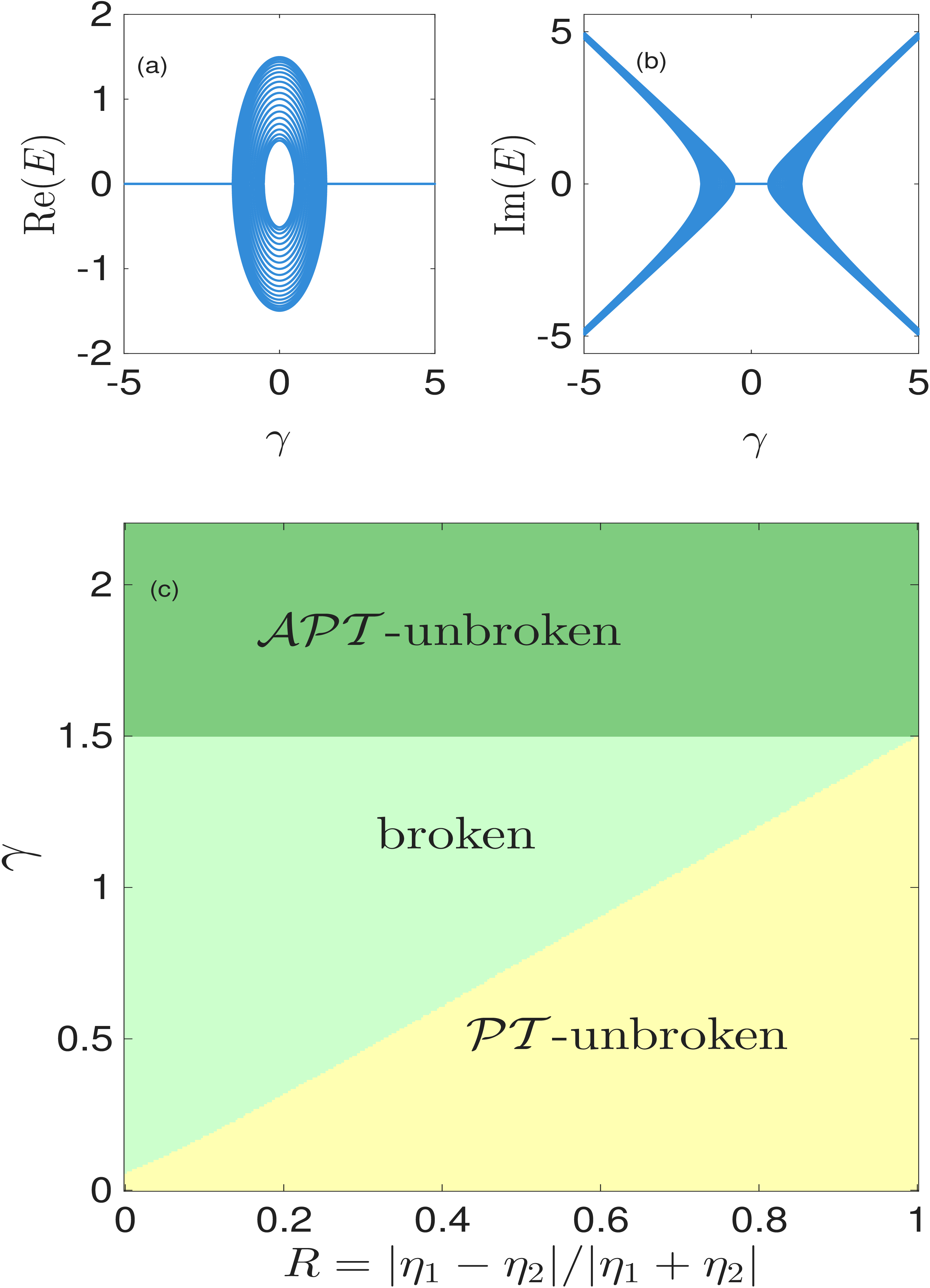
We numerically compute the energy spectrum of this Hamiltonian, as shown in Figs. 8 (a) and (b). As expected, the spectral behavior resembles that of the four-site model. As the non-Hermitian strength \(\gamma\) increases, the system undergoes a transition from a purely real spectrum to a purely imaginary one. The corresponding phase diagram is presented in Fig. 8 (c), which clearly demarcates the distinct parameter regions of the \(\mathcal{PT}\)-unbroken, symmetry broken, and \(\mathcal{APT}\)-unbroken phases, confirming that the multi-site lattice preserves the fundamental symmetries of the minimal unit cell.
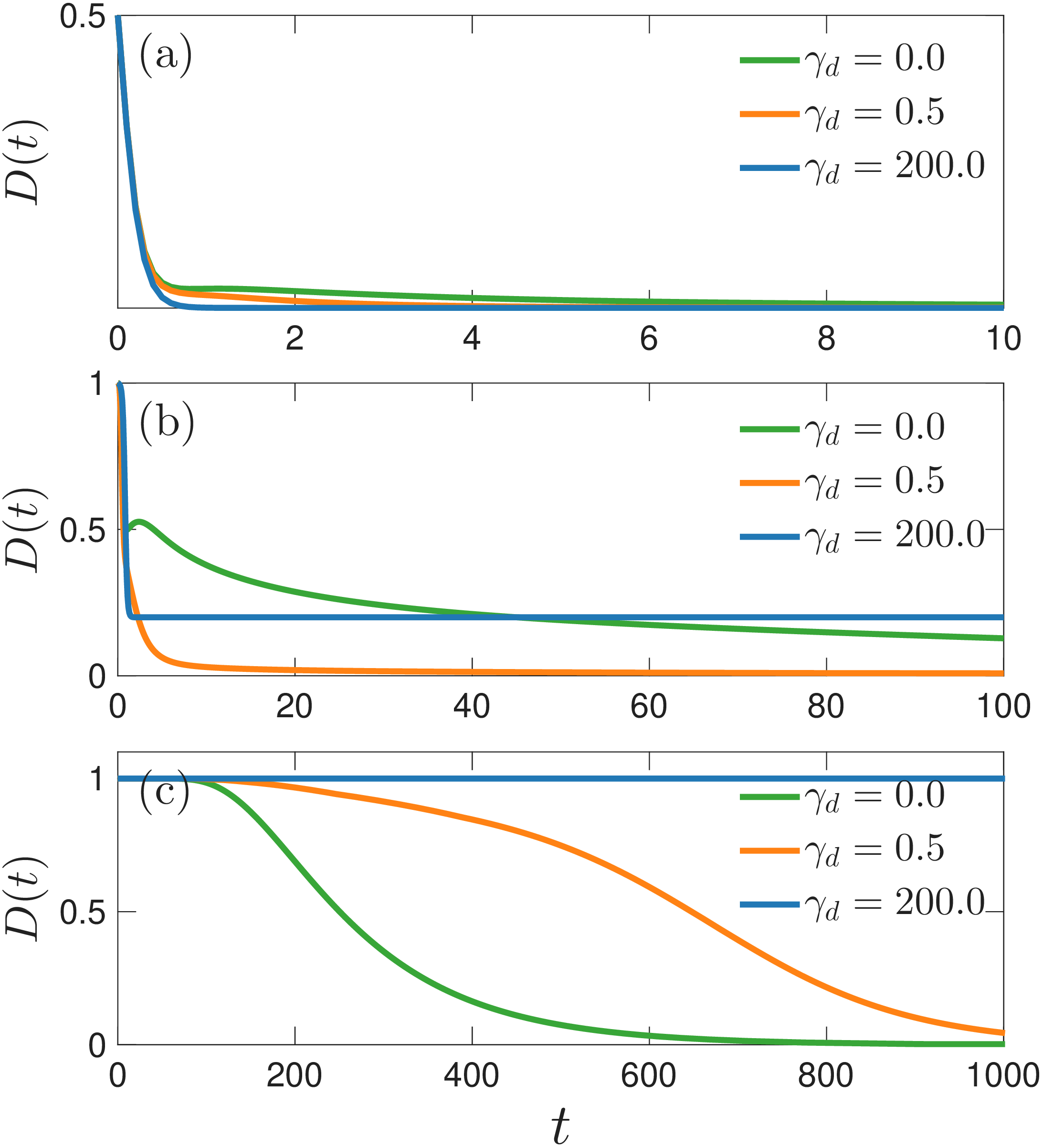
Crucially, we investigate the dynamical evolution of the trace distance \(D(t)\) under different pure dephasing strengths \(\gamma_d\), as shown in Fig. 9. Rather than observing a generic decay of quantum information due to the extensive size of the lattice, we find that the initial-state-dependent phenomena derived for the four-site model persist robustly in the 40-site chain. Specifically, Fig. 9 (a), with \(\hat{\rho}_1(0) = |S_1\rangle\langle S_1|\) and \(\hat{\rho}_2(0) = \frac{1}{2}(|S_1\rangle\langle S_1| + |S_2\rangle\langle S_2|)\), reproduces the accelerated decay (Case I). In Fig. 9 (b), we place the initial states deep within the bulk at adjacent gain and loss sites: \(\hat{\rho}_1(0) = |S_{17}\rangle\langle S_{17}|\) and \(\hat{\rho}_2(0) = |S_{18}\rangle\langle S_{18}|\). Even submerged in the 40-site lattice, strong dephasing isolates these sites from the rest of the chain, resulting in a partial stabilization of \(D(t)\) (Case II) to a finite stationary value in the long-time limit, effectively preventing complete information erasure. Finally, Fig. 9 (c) demonstrates complete stabilization (Case III). By initializing the states at gain sites, \(\hat{\rho}_1(0) = |S_1\rangle\langle S_1|\) and \(\hat{\rho}_2(0) = |S_{39}\rangle\langle S_{39}|\), strong dephasing completely severs any effective dynamic coupling across the extensive lattice, freezing the trace distance near its initial value. Overall, these results demonstrate that the initial-state-dependent dephasing effects and the dephasing-induced continuous protection mechanism in the \(\mathcal{APT}\) phase are highly scalable.
5 Conclusion↩︎
In summary, we have investigated the dynamical properties of non-Hermitian SSH models with alternating gain and loss in real space under the influence of local pure dephasing. By employing a quantum Lindblad master equation to describe the open-system dynamics, we characterized the evolution of the trace distance across different symmetry phases, including the \(\mathcal{PT}\)-unbroken, \(\mathcal{APT}\)-unbroken, and symmetry-broken regimes.
Our key finding is that the dynamical response of the trace distance to dephasing is largely determined by the initial state rather than by the underlying Hamiltonian symmetries. By varying the initial states, we identified three distinct dynamical behaviors that become pronounced in the strong-dephasing limit:
(i) Accelerated decay, where dephasing acts as a conventional detrimental noise source;
(ii) Partial stabilization, where the trace distance asymptotically approaches a finite, nonzero value in the long-time limit;
(iii) Complete stabilization, where the trace distance remains frozen at its initial value throughout the entire evolution.
By deriving effective linearized rate equations for the diagonal populations in the strong-dephasing limit, we established that these behaviors originate from the competition between non-Hermiticity-induced local amplification/decay and dephasing-induced spatial transport of population, which is initial-state dependent. Furthermore, in the \(\mathcal{APT}\)-unbroken phase, we observed an unconventional continuous suppression of the trace distance’s intrinsic decay upon increasing the dephasing strength. This protective mechanism is supported by the monotonic decrease of the Liouvillian gap. Finally, numerical simulations of a longer 40-site chain demonstrated that these initial-state-dependent dephasing effects scale robustly to extended multi-site systems.
These findings clarify the interplay between dephasing and non-Hermiticity with spatial gain and loss, demonstrating that initial-state engineering can be used to control or mitigate information loss. This work may offer useful insights for the design and realization of noise-resilient non-Hermitian quantum information processing devices in external environments.
This work is supported by the National Natural Science Foundation of China (Grant No. 12205179), the Shanghai Pujiang Program (Grant No. 22PJ1403900) and the Shanghai Science and Technology Innovation Action Plan (Grant No. 24LZ1400800).
6 Symmetry of the non-Hermitian SSH model↩︎
In this Appendix, we provide the detailed algebraic derivation of the symmetries for the non-Hermitian SSH Hamiltonian defined in Eq. 2 . We focus on the implementation of parity-time (\(\mathcal{PT}\)) and anti-parity-time (\(\mathcal{APT}\)) symmetries.
6.1 Parity-Time Symmetry↩︎
We first show that the Hamiltonian in Eq. (2 ) exhibits \(\mathcal{PT}\) symmetry. As defined in the main text, \(\mathcal{T}\) represents the usual time-reversal operation, and \(\mathcal{P}\) is the spatial inversion operator \(\hat{\sigma}_x \otimes \hat{\sigma}_x\), \[\mathcal{P} = \begin{pmatrix} 0 & 0 & 0 & 1 \\ 0 & 0 & 1 & 0 \\ 0 & 1 & 0 & 0 \\ 1 & 0 & 0 & 0 \end{pmatrix}.\] One can easily check that the following relation holds, \[\begin{align} \mathcal{P} \hat{H}^* \mathcal{P} &= \begin{pmatrix} 0 & 0 & 0 & 1 \\ 0 & 0 & 1 & 0 \\ 0 & 1 & 0 & 0 \\ 1 & 0 & 0 & 0 \end{pmatrix} \begin{pmatrix} -i\gamma & \eta_1 & 0 & 0 \\ \eta_1 & i\gamma & \eta_2 & 0 \\ 0 & \eta_2 & -i\gamma & \eta_1 \\ 0 & 0 & \eta_1 & i\gamma \end{pmatrix} \begin{pmatrix} 0 & 0 & 0 & 1 \\ 0 & 0 & 1 & 0 \\ 0 & 1 & 0 & 0 \\ 1 & 0 & 0 & 0 \end{pmatrix} \\ &= \begin{pmatrix} i\gamma & \eta_1 & 0 & 0 \\ \eta_1 & -i\gamma & \eta_2 & 0 \\ 0 & \eta_2 & i\gamma & \eta_1 \\ 0 & 0 & \eta_1 & -i\gamma \end{pmatrix} = \hat{H}. \end{align}\] namely, \(\mathcal{P} \hat{H}^* \mathcal{P} = \hat{H}\), where \(\hat{H}^*\) denotes the complex conjugate of \(\hat{H}\). This relation is equivalent to the commutation relation \([\hat{H},\mathcal{PT}]=0\), implying that the system is \(\mathcal{PT}\) symmetric. Hence, in the \(\mathcal{PT}\)-unbroken phase, the energy spectrum is purely real.
6.2 Anti-Parity-Time Symmetry↩︎
To see that the system also satisfies \(\mathcal{APT}\) symmetry, we define the parity operator \(\mathcal{P}'\) as \[\mathcal{P}' = \text{diag}(1, -1, 1, -1),\] which yields the following transformation \[\begin{align} \mathcal{P}' \hat{H}^* \mathcal{P}' &= \begin{pmatrix} 1 & 0 & 0 & 0 \\ 0 & -1 & 0 & 0 \\ 0 & 0 & 1 & 0 \\ 0 & 0 & 0 & -1 \end{pmatrix} \begin{pmatrix} -i\gamma & \eta_1 & 0 & 0 \\ \eta_1 & i\gamma & \eta_2 & 0 \\ 0 & \eta_2 & -i\gamma & \eta_1 \\ 0 & 0 & \eta_1 & i\gamma \end{pmatrix} \begin{pmatrix} 1 & 0 & 0 & 0 \\ 0 & -1 & 0 & 0 \\ 0 & 0 & 1 & 0 \\ 0 & 0 & 0 & -1 \end{pmatrix} \\ &= \begin{pmatrix} -i\gamma & -\eta_1 & 0 & 0 \\ -\eta_1 & i\gamma & -\eta_2 & 0 \\ 0 & -\eta_2 & -i\gamma & -\eta_1 \\ 0 & 0 & -\eta_1 & i\gamma \end{pmatrix} = -\hat{H}. \end{align}\] This relation is equivalent to the anti-commutation relation \(\{\hat{H},\mathcal{P'T}\}=0\). Hence, the system indeed respects \(\mathcal{APT}\) symmetry. In the \(\mathcal{APT}\)-unbroken phase, we expect a purely imaginary spectrum.
7 Elucidating decaying patterns of the trace distance in the \(\mathcal{APT}\)-unbroken phase↩︎
In Sec. 2 C of the main text, we unveiled rich decaying patterns of the trace distance in the \(\mathcal{APT}\)-unbroken phase of the closed non-Hermitian SSH model. Specifically, by simply tuning the initial-state pair \(\{\hat{\rho}_1(0), \hat{\rho}_2(0)\}\), one can observe two kinds of dynamical trends of the trace distance \(D(t)\): (i) Monotonic exponential decay, and (ii) non-monotonic decay. While the long-time asymptotic behavior is universally dictated by the slowest decay rate \(\Gamma_1-\Gamma_2\), the rich dynamical features at shorter timescales demand a deeper look. This Appendix presents a thorough theoretical analysis for these transient dynamics.
We begin by recalling the time evolution of the normalized density matrix, Eq. 6 in the main text \[\hat{\rho}(t) = \frac{\sum_{m,n}\rho_{mn}\,e^{-i(\lambda_m-\lambda_n)t}\,e^{(\Gamma_m+\Gamma_n)t}\,|\phi_m\rangle\langle\phi_n|}{\mathrm{Tr}\bigl[\sum_{m,n}\rho_{mn}\,e^{-i(\lambda_m-\lambda_n)t}\,e^{(\Gamma_m+\Gamma_n)t}\,|\phi_m\rangle\langle\phi_n|\bigr]}, \label{eq:rho95exact}\tag{30}\] where \(E_m = \lambda_m + i\Gamma_m\) (\(m \in \{1,2,3,4\}\)) are the complex eigenvalues of the non-Hermitian Hamiltonian \(\hat{H}\). The coefficients \(\rho_{mn} = \langle\chi_m|\hat{\rho}(0)|\chi_n\rangle\) represent the expansion components in the biorthonormal basis of \(\hat{H}\) defined by \(\langle\chi_m|\phi_n\rangle = \delta_{mn}\).
In the \(\mathcal{APT}\)-unbroken phase, the energy spectrum is purely imaginary, meaning \(\lambda_m = 0\) for all \(m\), and thus \(E_m = i\Gamma_m\). We order these imaginary parts in descending order: \(\Gamma_1 > \Gamma_2 > \Gamma_3 > \Gamma_4\). Due to the fact that the system also supports \(\mathcal{PT}\) symmetry, these eigenvalues are paired into \(\pm\) doublets \[\Gamma_4 = -\Gamma_1, \qquad \Gamma_3 = -\Gamma_2, \label{eq:pt95pairing}\tag{31}\] which leaves only two independent positive parameters: \(\Gamma_1 > \Gamma_2 > 0\).
To better isolate the relative decay rates, we factor out the dominant exponential term. By extracting \(e^{2\Gamma_1 t}\) from both the numerator and denominator of Eq. 30 , we can define a set of non-negative decay rates \[\Delta_m \equiv \Gamma_1 - \Gamma_m \ge 0. \label{eq:Delta95def}\tag{32}\] Utilizing the pairing symmetry in Eq. 31 , the explicit values of these rates are \(\Delta_1 = 0\), \(\Delta_2 = \Gamma_1 - \Gamma_2\), \(\Delta_3 = \Gamma_1 + \Gamma_2\), and \(\Delta_4 = 2\Gamma_1\). Consequently, the normalized density matrix simplifies to \[\hat{\rho}(t) = \frac{\displaystyle\sum_{m,n=1}^{4}\rho_{mn}\,e^{-(\Delta_m+\Delta_n)t}\,|\phi_m\rangle\langle\phi_n|}{\displaystyle\sum_{m,n=1}^{4}\rho_{mn}\,e^{-(\Delta_m+\Delta_n)t}\,N_{nm}}, \label{eq:rho95reduced}\tag{33}\] where \(N_{nm} \equiv \langle\phi_n|\phi_m\rangle\) represents the overlap matrix of the right eigenstates. Crucially, because \(\hat{H}\) is non-Hermitian, these eigenstates are generally non-orthogonal, meaning the off-diagonal elements are nonzero (i.e., \(N_{nm} \neq \delta_{nm}\)).
The full evolution in Eq. 33 is governed by the sum of exponents \(\Delta_m + \Delta_n\) across all 16 pairs of \((m,n) \in \{1,2,3,4\}^2\). Explicitly evaluating this matrix sum yields \[\renewcommand{\arraystretch}{1.5} \begin{array}{c|cccc} \Delta_m+\Delta_n & n=1 & n=2 & n=3 & n=4 \\\hline m=1 & 0 & \Gamma_1-\Gamma_2 & \Gamma_1+\Gamma_2 & 2\Gamma_1\\ m=2 & \Gamma_1-\Gamma_2 & 2(\Gamma_1-\Gamma_2) & 2\Gamma_1 & 3\Gamma_1-\Gamma_2\\ m=3 & \Gamma_1+\Gamma_2 & 2\Gamma_1 & 2(\Gamma_1+\Gamma_2) & 3\Gamma_1+\Gamma_2\\ m=4 & 2\Gamma_1 & 3\Gamma_1-\Gamma_2 & 3\Gamma_1+\Gamma_2 & 4\Gamma_1 \end{array} \label{tab:Delta95sum}\tag{34}\] By grouping the identical entries in this matrix, we find that the 16 combinations collapse into exactly nine distinct non-negative decay rates, denoted as \(\Omega_q\). Their corresponding multiplicities and specific \((m,n)\) pairings are summarized in Table 1.
| Rate \(\Omega_q\) | Multiplicity | \((m,n)\) pairs |
|---|---|---|
| \(0\) | 1 | \((1,1)\) |
| \(\Gamma_1-\Gamma_2\) | 2 | \((1,2),(2,1)\) |
| \(2(\Gamma_1-\Gamma_2)\) | 1 | \((2,2)\) |
| \(\Gamma_1+\Gamma_2\) | 2 | \((1,3),(3,1)\) |
| \(2\Gamma_1\) | 4 | \((1,4),(4,1),(2,3),(3,2)\) |
| \(3\Gamma_1-\Gamma_2\) | 2 | \((2,4),(4,2)\) |
| \(2(\Gamma_1+\Gamma_2)\) | 1 | \((3,3)\) |
| \(3\Gamma_1+\Gamma_2\) | 2 | \((3,4),(4,3)\) |
| \(4\Gamma_1\) | 1 | \((4,4)\) |
This mathematical decomposition offers a clear physical insight: a purely imaginary energy spectrum does not imply simple, single-exponential dynamics. Instead, due to the trace-normalization in the denominator, the state \(\hat{\rho}(t)\) behaves as a non-linear, fractional superposition of nine independent real exponential decay terms:
(i) In the long-time regime of \(t \to \infty\), all higher-rate channels rapidly die out. The system is universally dominated by the slowest available non-zero rate, \(\Omega = \Gamma_1 - \Gamma_2\), consistent with the observations in the main text.
(ii) In the short- and intermediate-time regimes, the remaining eight transient channels (\(\Omega_q > \Gamma_1 - \Gamma_2\)) remain active. Because the choice of initial states drastically alters the initial expansion coefficients \(\rho_{mn}\), it selectively activates or suppresses different decay channels. This multi-index competition between the nine channels is precisely what gives rise to the non-monotonic bumps, sharp dips, or purely monotonic decays observed in the trace distance.
8 Analytical Criterion for the Monotonicity of the Liouvillian Gap in the \(\mathcal{APT}\)-unbroken Phase↩︎
Here we examine when and under what conditions the Liouvillian gap decreases monotonically with increasing dephasing strength in the \(\mathcal{APT}\)-unbroken phase of the four-site non-Hermitian SSH system. To establish a rigorous criterion, it is sufficient to evaluate the sign of the initial slope (i.e., the derivative) of the Liouvillian gap at \(\gamma_d = 0\). Motivated by this, we investigate the weak-dephasing limit \(\gamma_d \to 0\). In the \(\mathcal{APT}\)-unbroken phase, the eigenvalues of the unperturbed Hamiltonian \(H\) are purely imaginary and are denoted as \(E = i\Gamma\). We present a self-contained, parameterized derivation based on first-order superoperator perturbation theory. This analytical framework systematically explains the transition between monotonic and nonmonotonic behavior of the Liouvillian gap as the dephasing strength increases.
Under a weak pure dephasing strength, the dynamics of the density matrix \(\hat{\rho}\) is governed by the total Liouvillian \(\mathcal{L}_0 = \mathcal{L}_1 + \gamma_d \mathcal{D}\), where the unperturbed part is \(\mathcal{L}_1[\hat{\rho}] = -i[\hat{H}\hat{\rho} - \hat{\rho}\hat{H}^\dagger]\), and the dephasing superoperator takes the standard form \(\mathcal{D}[\hat{\rho}] = \sum_{k} \hat{L}_k \hat{\rho} \hat{L}_k - \hat{\rho}\). At \(\gamma_d = 0\), as evidenced by the exact time evolution of the density matrix in Eq. 30 , the relaxation rates of the eigenmodes \(|\phi_m\rangle\langle\phi_n|\) are dictated by the sum of the imaginary parts of the corresponding Hamiltonian eigenvalues, \(\Gamma_m + \Gamma_n\). Denoting the two relevant imaginary parts as \(\Gamma_1\) and \(\Gamma_2\) (with \(\Gamma_1 > \Gamma_2\)), the slowest relaxation rate is explicitly \(\mathcal{E}^{(0)}_1 = 2\Gamma_1\) (arising from \(m=n=1\)). The second slowest rate is \(\mathcal{E}^{(0)}_2 = \Gamma_1 + \Gamma_2\), which corresponds to the twofold degenerate subspace (\(m=1, n=2\) and \(m=2, n=1\)). Consequently, the unperturbed Liouvillian gap is determined by the difference between these two leading rates: \[\Delta\mathcal{E}^{(0)} = \mathcal{E}^{(0)}_1 - \mathcal{E}^{(0)}_2 = 2\Gamma_1 -(\Gamma_1 + \Gamma_2) = \Gamma_1 - \Gamma_2.\]
To include the first-order correction from \(\gamma_d \mathcal{D}\) in the weak dephasing limit, we need the explicit biorthogonal eigenstates of the four-site Hamiltonian \(H\) [Eq. 2 ]. We begin by recalling its characteristic equation. Defining the auxiliary variable \(\xi \equiv \gamma^2 + E^2 = \gamma^2 - \Gamma^2\), the secular equation \(\det(E\hat{I} - \hat{H}) = 0\) reduces to a quadratic form in \(\xi\), \[\xi^2 - (2\eta_1^2 + \eta_2^2)\xi + \eta_1^4 = 0. \label{eq:secular95u}\tag{35}\] The two roots correspond exactly to \(\xi_1 = u_-\) and \(\xi_2 = u_+\) defined below Eq. (3 ). We have \(\Gamma_m = \sqrt{\gamma^2 - \xi_m}\) (\(m \in \{1,2\}\)).
To explicitly calculate the spatial distribution of the unperturbed density matrix, we must first construct the biorthogonal weights \(\mathbf{w}\) on each site, defined by \(w_n = \chi_n \phi_n\). Since the non-Hermitian Hamiltonian in Eq. 2 inherently satisfies the transposition symmetry \(\hat{H}^T = \hat{H}\), its left and right eigenstates are simply related by the transpose operation, i.e., \(\langle \chi_m | = |\phi_m\rangle^T\). Physically, in the \(\mathcal{APT}\)-unbroken phase (where energies \(E = i\Gamma\) are purely imaginary), the non-Hermitian nature of the system locks the relative phase between different sublattices. When we square the wavefunction to compute the weight \(w_n = \phi_n^2\), this phase factor is squared as well, i.e., \((-i)^2 = -1\). This naturally explains why the unnormalized weights at the lossy sites must be negative.
To express this density distribution cleanly without carrying complex numbers through our calculations, we can directly parameterize the state using purely real variables. For each eigenmode (\(m \in \{1,2\}\)), we define two dimensionless parameters: \[y_m \equiv \frac{\xi_m}{\eta_1^2}, \quad v_m \equiv \frac{\gamma - \Gamma_m}{\gamma + \Gamma_m}.\] Applying these real parameters, the unnormalized biorthogonal weight vector \(\mathbf{w}^{(m)} = [w_a^{(m)}, w_b^{(m)}, w_c^{(m)}, w_d^{(m)}]^T\) emerges in a compact form. The negative signs explicitly manifest at the second and fourth sites as a direct consequence of the aforementioned \((-i)^2\) operation: \[\mathbf{w}^{(m)} = \begin{pmatrix} 1 \\ -v_m y_m \\ y_m \\ -v_m \end{pmatrix}.\] The corresponding biorthogonal norm \(N_m \equiv \sum_{n} w_n^{(m)}\) is then gracefully factored as \(N_m = (1 - v_m)(1 + y_m)\). Consequently, the normalized biorthogonal density distribution \(P^{(m)} \equiv \mathbf{w}^{(m)} / N_m\) on the four sites is given analytically by \[P^{(m)} = \frac{1}{(1-v_m)(1+y_m)} \begin{pmatrix} 1 \\ -v_m y_m \\ y_m \\ -v_m \end{pmatrix}, \label{eq:normalized95P}\tag{36}\] which strictly satisfies the normalization condition \(\sum_{n} P_n^{(m)} = 1\).
With the expressions for the biorthogonal density distributions \(P^{(m)}\) established, we are now equipped to evaluate the dephasing-induced corrections to the Liouvillian spectrum. As evidenced by Eq. 30 , the \(\mathcal{E}^{(0)}_2 = \Gamma_1 + \Gamma_2\) is twofold degenerate. To calculate the first-order dephasing-induced correction to this degenerate subspace, we employ degenerate perturbation theory. We construct a \(2 \times 2\) perturbation matrix \(V\) in the subspace spanned by the right eigenoperators \(|R_A\rangle\rangle = |\phi_1\rangle\langle\phi_2|\), \(|R_B\rangle\rangle = |\phi_2\rangle\langle\phi_1|\) and their left counterparts \(\langle\langle L_A| = (|\chi_1\rangle\langle\chi_2|)^\dagger\), \(\langle\langle L_B| = (|\chi_2\rangle\langle\chi_1|)^\dagger\), where \(|\chi_m\rangle\) denote the left eigenstates of \(H\) biorthonormalized as \(\langle\chi_m|\phi_n\rangle = \delta_{mn}\). The matrix elements are defined as \(V_{\alpha\beta} = \langle\langle L_\alpha | \mathcal{D} | R_\beta \rangle\rangle\) for \(\alpha, \beta \in \{A, B\}\).
Using the biorthogonal properties, the diagonal elements of \(V\) are given by \[V_{AA} = V_{BB} = \sum_{n=1}^4 P_n^{(1)} P_n^{(2)} - 1.\] The off-diagonal elements describing the dephasing-induced coupling between the two degenerate channels are calculated as \[V_{AB} = V_{BA} = \sum_{n=1}^4 P_n^{(1)} P_n^{(2)}.\] By defining the cross-overlap integral as \(C \equiv \sum_{n} P_n^{(1)} P_n^{(2)}\), the perturbation matrix can be compactly written as \[V = \begin{pmatrix} C - 1 & C \\ C & C - 1 \end{pmatrix}.\] Solving the secular equation \(\det(V - E^{(1)} I) = 0\), the degenerate eigenvalue splits into two branches \[E^{(1)}_- = -1, \quad E^{(1)} _+= 2C - 1 = 2 \sum_{n=1}^4 P_n^{(1)} P_n^{(2)} - 1.\] Since \(C > 0\), the branch \(E^{(1)}_+\) has a larger real part and corresponds to the physical perturbed second largest decay rate of the system, which yields its first-order correction \(\delta\mathcal{E}_2 = E^{(1)}_+\).
Since the maximum \(\mathcal{E}^{(0)}_1 = 2\Gamma_1\) is non-degenerate, its first-order correction is \(\delta\mathcal{E}_1 = \sum_n (P_n^{(1)})^2 - 1\). Under the degenerate perturbation framework, the first-order derivative of the Liouvillian gap at the weak-dephasing limit is analytically defined as \[\label{eq:c10} \zeta = \left. \frac{d\Delta\mathcal{E}}{d\gamma_d} \right| _{\gamma_d = 0} = \delta\mathcal{E}_1 - \delta\mathcal{E}_2 = \sum_{n=1}^4 (P_n^{(1)})^2 - 2 \sum_{n=1}^4 P_n^{(1)} P_n^{(2)}.\tag{37}\] To evaluate \(\zeta\), we apply Vieta’s formulas to the secular equation Eq. 35 . The relations between the roots \(\xi_1\) and \(\xi_2\) yield \[\begin{align} \xi_1 \xi_2 &= \eta_1^4 \implies y_1 y_2 = 1, \tag{38} \\ \xi_1 + \xi_2 &= 2\eta_1^2 + \eta_2^2 \implies y_1 + y_2 = 2 + \frac{\eta_2^2}{\eta_1^2}. \tag{39} \end{align}\] Eq. 38 indicates that the dimensionless factors of the two modes are reciprocal to each other.
Substituting \(y_2 = 1/y_1\) into the term \(P^{(1)} \cdot P^{(2)}\) [cf. Eq. 36 ], we obtain \[P^{(1)} \cdot P^{(2)} = \frac{2(1 + v_1 v_2) y_1}{(1-v_1)(1-v_2)(1+y_1)^2}.\] Similarly, the self-overlap term \(P^{(1)} \cdot P^{(1)}\) is expressed as \[P^{(1)} \cdot P^{(1)} = \frac{(1 + v_1^2) y_1 \left(2 + \frac{\eta_2^2}{\eta_1^2}\right)}{(1-v_1)^2 (1+y_1)^2}.\]
Inserting the above two results into Eq. (37 ) and factoring out the strictly positive common term \(\frac{y_1}{(1+y_1)^2 (1-v_1)}\). The sign of the initial slope \(\zeta\) is then uniquely determined by the \(K\) \[\zeta \propto K = \frac{1 + v_1^2}{1 - v_1} \left( 2 + \frac{\eta_2^2}{\eta_1^2} \right) - \frac{4(1 + v_1 v_2)}{1 - v_2}. \label{eq:discriminant}\tag{40}\] The analytical discriminant \(K\) in Eq. 40 elegantly captures the competition between the system parameters (\(\eta_1, \eta_2, \gamma\)). Crucially, the sign of \(K\) dictates the evolutionary trajectory of the Liouvillian gap under weak dephasing. Specifically, when \(K > 0\), the initial slope \(\zeta\) is positive, indicating that the Liouvillian gap initially increases, which inherently leads to a non-monotonic behavior as it must eventually decrease at strong dephasing. Conversely, when \(K < 0\), \(\zeta\) is negative, indicating that the dephasing processes immediately drive a monotonic decrease of the gap.