A Synthetic Reliability-Aware PINN Benchmark for Offshore Wind Turbine Support-Structure Monitoring with Bayesian Inverse Identification
June 23, 2026
Abstract
Reliable structural health monitoring (SHM) of offshore wind turbine (OWT) support structures requires fast state estimation from sparse measurements. Repeated high-fidelity finite-element or aeroelastic analyses are difficult to use directly in online monitoring loops, while purely data-driven surrogates can require large training sets. This paper presents DigiTurbine, a synthetic reliability-aware Physics-Informed Neural Network (PINN) benchmark for OWT monopile support-structure monitoring. The workflow embeds a simplified Euler–Bernoulli beam equation with Winkler soil foundation in the training objective, couples it with Bayesian-prior-informed inverse identification, and adds First-Order Reliability Method (FORM) screening. All validation uses synthetic configurations with analytical or finite-difference ground truth motivated by the NREL 5 MW reference turbine context.
Three contributions are evaluated. (1) Forward PINN: A 4,353-parameter network with EMA-adaptive loss weighting achieves mean RMSE \(0.135 \pm 0.109\) mm (10/10 pass) with all-configuration mean inference of 0.381 ms (GPU) / 0.605 ms (CPU), 26\(\times\) / 17\(\times\) below the 10 ms real-time target. (2) Inverse PINN and gradient direction problem: Standard simultaneous optimisation of network weights and unknown parameters (\(E\), \(k_\text{soil}\)) fails on the tested 4th-order PDE inverse cases because of conflicting gradient directions (mean error 63.9 %, 0/4 pass), and five loss-weighting or scheduling mitigations also fail in the large-offset synthetic tests. A weak log-normal Bayesian prior centred on the correct design/as-built specification substantially mitigates this failure on the tested cases: 8/8 pass, mean \(E\) error \(\leq 0.02\) %, including simultaneous \(E{+}k_\text{soil}\) identification under 10 % measurement noise. (3) Near-real-time reliability: The FORM layer solves representative structural limit-state cases in 0.7–2.7 ms, with the OWT cantilever root-moment capacity case requiring about 1.0 ms (\(>\)40\(\times\) faster than Monte Carlo), machine-precision agreement for linear limit states, and \(\leq 6\) % error for moderately nonlinear cases. In the benchmarked synthetic workflow, the online pipeline completes in \(<\)7 ms, giving theoretical processing headroom for SCADA-style monitoring.
Physics-Informed Neural Networks ,Synthetic Benchmark ,Digital Twin , Offshore Wind Turbine ,Structural Health Monitoring , Bayesian Inverse Identification ,Gradient Direction Problem , First-Order Reliability Method ,Euler–Bernoulli Beam
1 Introduction↩︎
Global wind installations reached a record 165 GW in 2025, taking total installed wind capacity to 1,299 GW, while offshore wind reached 92.5 GW by the end of 2025 after 9.3 GW of new offshore capacity was grid-connected [1], [2]. Continued renewable expansion is expected toward 2030 [3]. Fixed-bottom support structures, especially monopiles, remain central to deployed offshore wind and must endure \(10^8\)–\(10^9\) fatigue cycles over a 25-year service life, making fatigue a dominant structural design concern [4]–[6]. Operations and maintenance (O&M) costs represent 25–30 % of lifecycle expenditure, and published condition-based monitoring studies report potential O&M savings of 11–18 % [7]. Yet structural sensing remains sparse, often limited to small sets of accelerometer and strain measurements [5], [7], [8], making real-time full-field structural state inference from sparse, noisy data a fundamental challenge.
Physics-Informed Neural Networks (PINNs) [9] encode governing PDEs as soft loss constraints, enabling sparse-data surrogates in solid mechanics and wind-energy applications [10], [11]. The present study tests the 50–100 measurement regime, far fewer than would typically be expected for purely data-driven surrogates. Extended to inverse problems, PINNs treat unknown material properties as additional optimisation variables; however, a gradient direction problem, not systematically characterised in the reviewed literature, prevents convergence in the tested cases when parameters are initialised far from their true values. Digital Twins (DTs) at Level 2–3 maturity [12], [13] couple physics-based surrogates with reliability analysis for continuous structural prognostics. First-Order Reliability Method (FORM) [8] estimates the reliability index \(\beta(t)\) through constrained optimisation and is typically far cheaper than Monte Carlo for low-dimensional limit states; paired with PINN-updated structural estimates, it enables near-real-time reliability screening not found in the reviewed OWT DT literature.
1.1 Research Gaps↩︎
A focused review of recent PINN, digital-twin, reliability, and OWT structural monitoring studies identifies four open gaps; representative studies are shown in Table 1.
Computational gap. High-fidelity FEA can require minutes to hours per evaluation; pure ML requires thousands of training samples. No OWT SHM framework in the reviewed literature was found to achieve sub-10 ms physics-consistent inference from sparse data.
Inverse problem gap. Published inverse PINNs do not study convergence failure under large-offset initialisations. The gradient direction problem was not found to be identified, formally analysed, or substantially mitigated in the reviewed literature.
Integration gap. Within the reviewed literature, no prior work was found to integrate PINN forward prediction, inverse parameter identification, and probabilistic reliability in a single synthetic-data-validated OWT pipeline.
Reliability speed gap. Monte Carlo can be too slow for repeated online reliability updates, particularly when coupled to high-fidelity structural models; FORM integrated with a physics-consistent PINN state-estimation workflow was not found for OWT structures in the reviewed literature.
1.2 Contributions↩︎
This paper makes the following specific contributions, evaluated using synthetic benchmark experiments.
Forward PINN for OWT monopile: PDE-constrained surrogate for a simplified Euler–Bernoulli/Winkler monopile benchmark (a Morison forcing helper is implemented in
morison_force(), but Morison-driven PINN training is deferred to future field-calibration work), evaluated across 10 synthetic uniform-load configurations. Mean RMSE \(0.135 \pm 0.109\) mm, all-configuration mean inference 0.381 ms (GPU) / 0.605 ms (CPU) (both well below the 10 ms target); 10/10 test cases pass from only 50–100 sparse measurements.Gradient direction problem: identification, analysis, and Bayesian mitigation. Formal gradient analysis and experimental characterisation of the circular-dependency failure in standard inverse PINNs for high-order PDEs. Five mitigation strategies all fail without priors. Weak Bayesian priors centred on the correct design/as-built specifications achieve 8/8 success, mean \(E\) error \(\leq 0.02\) %, including simultaneous \(E + k_\text{soil}\) identification under 10 % noise.
FORM reliability layer within the PINN workflow: representative FORM solves in 0.7–2.7 ms, with the OWT cantilever root-moment capacity case at about 1.0 ms (\(>40\times\) faster than Monte Carlo); machine-precision accuracy for linear limit states; \({\leq}6\,\%\) error for moderately nonlinear cases. DigiTurbine end-to-end pipeline: \(<\)7 ms, corresponding to \(>\)143 Hz theoretical processing headroom.
2 Literature Review↩︎
2.1 Digital Twins and PINNs for OWT↩︎
Digital twin applications to OWT have grown rapidly, covering fleet-level SCADA analytics [14], component-level SHM [7], Bayesian reliability updating from monitoring data [5], probabilistic risk-based inspection planning [15], and mooring-line monitoring [16]. Wang et al.[6] conducted a comprehensive review of OWT support-structure reliability within a DT context, concluding that no ML- or PINN-based framework existed for integrated reliability monitoring. Chiachío et al.[17] and Ritto & Rochinha [13] developed DT frameworks with Bayesian updating and physics-based ML classifiers respectively, but without PINN-based millisecond inference. Chen et al.[18] reviewed floating-OWT DTs using hybrid neural surrogates; Lai et al.[19] demonstrated fatigue monitoring in aircraft wings via measurement–computation fusion; both lack real-time reliability metrics.
PINNs [9], [20] have been applied to solid-mechanics material identification [10], wind-farm wake dynamics [21], wind-turbine bearing fatigue [22], wind-turbine power prediction with uncertainty quantification [23], and monopile scour detection from natural-frequency shifts [11]. These works collectively establish PINNs as viable for wind-energy applications, but the reviewed works do not address convergence failure of inverse PINNs or integrate structural reliability analysis.
2.2 Inverse PINNs and Structural Reliability↩︎
Standard inverse PINNs co-optimise network weights and unknown physical parameters via a PDE-constrained loss [9]. Applications to bearing diagnostics [24] and elasticity identification [10] report success but generally do not systematically stress-test large-offset initialisations. Offshore SHM can involve substantial parameter uncertainty from material degradation, scour, and soil–structure changes; convergence under such conditions remains underexplored. Published works report successful cases without examining failure mechanisms, and no systematic study of convergence under varied initialisations or noise levels was found. In particular, the gradient direction problem (large-error failure from circular dependencies between unknown parameters and high-order network derivatives) has not previously been identified, characterised, or substantially mitigated in the reviewed literature.
Structural reliability for OWT has been addressed via FORM, SORM, and Monte Carlo [8], [25], but probabilistic analysis remains computationally intractable for continuous monitoring at FEA speeds. FORM integrated with a physics-consistent PINN state-estimation workflow for real-time \(\beta(t)\) was not found in the reviewed literature for OWT support structures.
2.3 Gap Matrix and Positioning↩︎
Table 1 presents a positioning matrix across the reviewed literature. The bottom row summarises the limited-scope combination implemented in this synthetic benchmark.
| Reference | Venue / Year | DT | PINN | Reliability | OWT Struct. | Inverse |
|---|---|---|---|---|---|---|
| Leon-Medina et al.[7] | Intell. Syst. Appl. | ✔ | ML only | Component | ✔ | – |
| Ambarita et al.[14] | Energy Inform. | ✔ | – | – | ✔ | – |
| Chen et al.[18] | Energies 2024 | \(\sim\) | Hybrid | Qualitative | Floating | – |
| Augustyn et al.[5] | Energies 2021 | ✔ | – | Bayesian | ✔ | – |
| Bull et al.[15] | Struct. Health Monit. | ✔ | – | Risk-based | ✔ | – |
| Walker et al.[16] | J. Ocean Eng. | ✔ | – | Component | Mooring | – |
| Qin et al.[24] | Knowl.-Based Syst. | ✔ | Inverse | Diagnostics | – | ✔ |
| Zhang & Zhao [21] | En. Conv. Mgmt. | ✔ | Farm | – | ✔ | – |
| Chen et al.[11] | Ocean Eng. | – | Forward | – | Monopile | \(\sim\) |
| Das et al.[25] | Comput. Struct. | – | Bayesian | General | – | – |
| Chiachio et al.[17] | Autom. Constr. | ✔ | – | \(\sim\) | – | – |
| Ritto & Rochinha [13] | Mech. Syst. Signal 2021 | ✔ | ML class. | – | ✔ | – |
| Lai et al.[19] | J. Manuf. Syst. | ✔ | – | Fatigue | – | – |
| Wang et al.[6] | Ocean Eng. | \(\sim\) | – | Review | ✔ | – |
| Yucesan & Viana [22] | Appl. Soft Comput. | ✔ | ✔ | Bearing | Component | – |
| This work | Synthetic benchmark | Synth. DT | Fwd.+inv. PINN | FORM | 1D monopile | Bayes prior |
3pt
3 Theoretical Framework↩︎
3.1 Structural Mechanics of the OWT Monopile↩︎
3.1.1 Euler–Bernoulli Beam with Winkler Foundation↩︎
The transverse vibration of a monopile section is governed by the Euler–Bernoulli partial differential equation in the presence of viscous damping, distributed loading, and Winkler soil reaction:
\[\begin{align} EI\,\frac{\partial^4 u}{\partial x^4} &+ k_{\text{soil}}(x)\,u + c\,\frac{\partial u}{\partial t} \\ &+ \rho A\,\frac{\partial^2 u}{\partial t^2} = q(x,t), \end{align} \label{eq:EB}\tag{1}\]
where \(x \in [0,L]\) is the axial coordinate, \(t\) is time, \(u(x,t)\) is the transverse displacement (m), \(EI\) is the bending stiffness (Pa m\(^4\)), \(\rho A\) is the linear mass (kg m\(^{-1}\)), \(c\) is the distributed damping coefficient (N s m\(^{-2}\)), \(k_\text{soil}\) is the equivalent Winkler foundation stiffness per unit beam length used in the one-dimensional beam equation (N m\(^{-2}\)), and \(q(x,t)\) is the distributed transverse load (N m\(^{-1}\)).
For the NREL 5 MW reference turbine [26] the relevant nominal properties are: pile outer diameter \(D = 6.0\) m, wall thickness \(t_w = 0.06\) m, Young’s modulus \(E = 210\) GPa, density \(\rho = 7{,}850\) kg m\(^{-3}\), cross-sectional area \(A = 1.13\) m\(^2\), second moment of area \(I = 4.94\) m\(^4\), and pile embedment depth 30 m. These properties are cited for physical context of the NREL 5 MW reference turbine; the validation experiments in Section 5 use a representative simplified beam model (\(I = 8.333 \times 10^{-3}\) m\(^4\), \(A = 0.05\) m\(^2\), \(EI = 1.75\) GN m\(^2\)) that produces well-resolved millimetre-scale deflections, enabling exact ground-truth comparison with the analytical solution (Eq. 3 ). Representative geotechnical subgrade moduli range from 5 MN m\(^{-3}\) (loose sand) to 60 MN m\(^{-3}\) (dense sand or stiff clay) according to DNV-ST-0126 [4], [8]. When used in Eq. 1 , these values are converted to an equivalent per-length beam stiffness by multiplying by an effective pile width or diameter.
Boundary conditions for a clamped-base (pile–soil interface), free-top cantilever: \[\begin{gather} u(0,t) = 0, \quad u_x(0,t) = 0, \\ EI\,u_{xx}(L,t) = 0, \quad EI\,u_{xxx}(L,t) = 0. \end{gather} \label{eq:BC}\tag{2}\]
Figure 1 illustrates the simplified monopile model used in this study, showing the clamped base, soil reaction, distributed loading, and sparse displacement measurement locations.
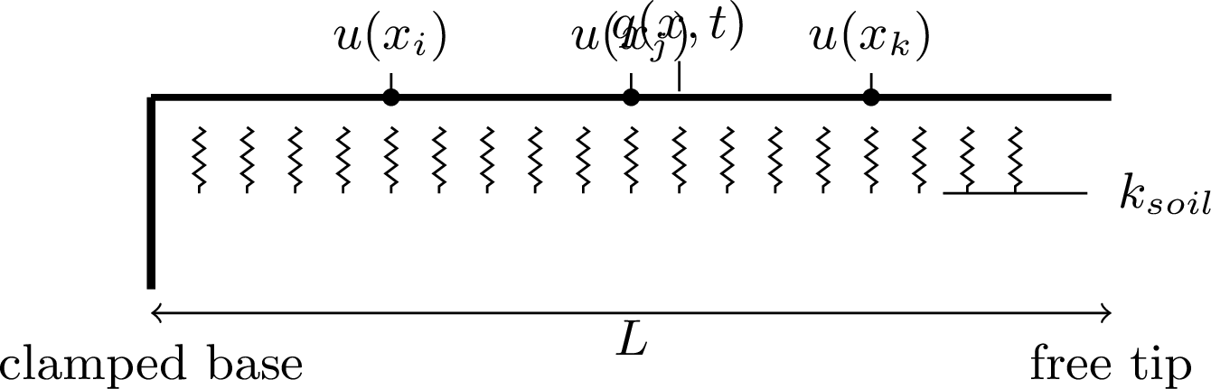
The analytical static solution for a uniformly distributed load \(q\) on a clamped-free beam without soil interaction (used for validation): \[\begin{align} u(x) &= \frac{q x^2}{24EI}\bigl(6L^2 - 4Lx + x^2\bigr). \end{align} \label{eq:analytical}\tag{3}\] This expression provides exact ground truth for the no-soil static beam cases; finite-difference Winkler-beam references are used for the soil-interaction inverse cases.
3.1.2 Morison Hydrodynamic Loading↩︎
Wave loading on the sub-surface monopile section can be represented by the Morison equation [27]: \[q_{\text{wave}}(x,t) = \tfrac{1}{2}\rho_w C_D D|v_w|v_w + \rho_w C_M \tfrac{\pi D^2}{4}\dot{v}_w,
\label{eq:morison}\tag{4}\] where \(\rho_w = 1{,}025\) kg m\(^{-3}\), \(C_D \in [0.6,1.2]\), and \(C_M \in
[1.2,2.0]\). The current implementation (morison_force()) is a simplified Morison forcing helper used for software validation; Airy/JONSWAP wave-kinematics coupling and full aero-elastic Morison-driven training are deferred to future
field-calibration work.
3.2 PINN Formulation↩︎
3.2.1 Composite Loss Function↩︎
A PINN approximates \(u(x,t)\) with a multilayer perceptron \(\hat{u}(x,t;\theta)\) parameterised by trainable weights \(\theta\). The training objective is the weighted composite loss:
\[\mathcal{L}(\theta) = \lambda_{\text{data}}\,\mathcal{L}_{\text{data}}(\theta) + \lambda_{\text{PDE}}\,\mathcal{L}_{\text{PDE}}(\theta) + \lambda_{\text{BC}}\,\mathcal{L}_{\text{BC}}(\theta), \label{eq:losstotal}\tag{5}\]
where the three loss components are defined as follows.
Data loss (fit to sparse sensor observations): \[\mathcal{L}_{\text{data}}(\theta) = \frac{1}{N_d}\sum_{i=1}^{N_d} \bigl[\hat{u}(x_i,t_i;\theta) - u_i^{\text{obs}}\bigr]^2. \label{eq:Ldata}\tag{6}\]
PDE residual loss (enforce Euler–Bernoulli equation at \(N_f\) collocation points uniformly distributed throughout the domain): \[\begin{align} \mathcal{L}_{\text{PDE}}(\theta) &= \frac{1}{N_f}\sum_{j=1}^{N_f} \Bigl[EI\,\hat{u}_{xxxx,j} + k_\text{soil}\,\hat{u}_j \\ &\quad + c\,\dot{\hat{u}}_j + \rho A\,\ddot{\hat{u}}_j - q_j\Bigr]^2, \end{align} \label{eq:Lphys}\tag{7}\] where subscript \(j\) denotes evaluation at \((x_j,t_j;\theta)\). The implementation evaluates the same residual in normalised coordinates and rescales the residual terms for stable optimisation.
Boundary condition loss (enforce Eq. 2 at domain boundaries): \[\begin{align} \mathcal{L}_{\text{BC}}(\theta) &= \bigl[\hat{u}(0;\theta)\bigr]^2 + \bigl[\hat{u}_x(0;\theta)\bigr]^2 \\ &\quad + \bigl[\hat{u}_{xx}(L;\theta)\bigr]^2 + \bigl[\hat{u}_{xxx}(L;\theta)\bigr]^2. \end{align} \label{eq:Lbc}\tag{8}\] The zero-valued moment and shear conditions in Eq. 2 are therefore enforced through the corresponding derivative residuals.
All neural-network partial derivatives in Eqs. 7 –8 are computed by PyTorch automatic differentiation [28], avoiding finite-difference derivative approximations at the collocation points. The PDE residual \(\mathcal{L}_\text{PDE}\) evaluated at 200 collocation points provides dense structural information that functions as a physics-based data augmentation.
3.2.2 Exponential Moving Average Adaptive Loss Weighting↩︎
Fixed loss weights caused one component to dominate in 3/10 configurations. This study uses EMA-adaptive weighting with running averages \[\bar{\mathcal{L}}_i^{(t)} = (1-\alpha)\,\bar{\mathcal{L}}_i^{(t-1)} + \alpha\,\mathcal{L}_i^{(t)}, \label{eq:ema}\tag{9}\] and dynamic weights \(\lambda_i^{(t)} = \bar{\mathcal{L}}_\text{avg}^{(t)}/\bigl(\bar{\mathcal{L}}_i^{(t)}+\varepsilon\bigr)\), with \(\alpha{=}0.02\), \(\varepsilon{=}10^{-6}\), which balances component scales by down-weighting persistently large-magnitude losses and up-weighting smaller-magnitude components.
3.3 First-Order Reliability Method↩︎
Given a limit-state function \(g(\mathbf{X}) \leq 0\) defining failure and \(n\) standard-normal variables \(U_i = (X_i - \mu_i)/\sigma_i\), with \(\mathbf{X}=T^{-1}(\mathbf{u})\) denoting the transformation from standard normal space to physical variables, FORM defines the reliability index \[\beta = \min_{\mathbf{u}:\,g(T^{-1}(\mathbf{u}))=0} \|\mathbf{u}\|_2 \label{eq:beta}\tag{10}\] and approximates failure probability as \(P_f \approx \Phi(-\beta)\) [8]. The Most Probable Point is located via SLSQP in 5–15 function evaluations. In the benchmarked implementation, SLSQP evaluates user-defined algebraic limit-state functions and estimates the required local sensitivities numerically by finite differences. Coupling the optimiser directly to a trained PINN displacement evaluator is compatible with the same interface but is not separately benchmarked in this paper.
4 Methodology↩︎
4.1 System Architecture Overview↩︎
Fig. 2 illustrates the two-phase DigiTurbine monitoring workflow.
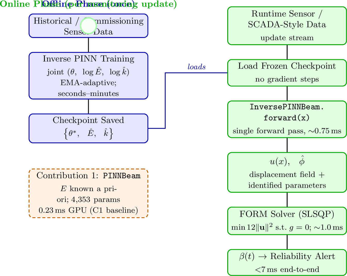
The system operates in two phases. Offline: the Inverse PINN is trained on historical or commissioning sensor data (seconds to a few minutes in the present experiments); all model weights \(\theta^*\)
and identified parameters \(\hat{\phi}\) are saved to a checkpoint. Online: at every monitoring update the frozen checkpoint is loaded and a single forward pass (\(\sim\)0.75 ms) yields both the full displacement field \(u(x)\) and the stored parameter estimates. FORM then evaluates the selected structural limit state using these updated state estimates;
the reported OWT cantilever case requires about 1.0 ms. No retraining occurs during online operation; periodic offline retraining (e.g.after a storm event or on a monthly schedule) refreshes \(\hat{\phi}\) using new sensor
history. When \(E\) is known in advance, the lightweight Forward PINN (PINNBeam, 4,353 parameters) provides full-field reconstruction at 0.23 ms for the C1 baseline and serves as the standalone Contribution 1
benchmark.
The software implementation uses a modular backend comprising PINNBeam, InversePINNBeam, FORMSolver, and a Streamlit real-time monitoring dashboard.
4.2 Forward PINN Design and Training↩︎
4.2.1 Network Architecture↩︎
The network is a 2-hidden-layer MLP with 64 neurons per layer: \[\hat{u} = \mathcal{N}_\theta:\; \mathbb{R} \ni x \;\longmapsto\; \hat{u} \in \mathbb{R}.\] The \(\tanh\) activation is used because it provides \(\mathcal{C}^\infty\) smoothness, and in particular \(\mathcal{C}^4\) continuity in the \(x\) direction needed for accurate computation of \(\partial^4\hat{u}/\partial x^4\) via automatic differentiation. ReLU-type activations are unsuitable for this fourth-order PINN because their higher derivatives are zero or ill-defined over much of the domain. Hidden layers use PyTorch default initialisation (Kaiming uniform); the output layer uses small-norm initialisation (\(\text{std}=10^{-3}\), zero bias) for stable initial predictions near zero. The parameter count is \(1{\times}64 + 64{\times}64 + 64{\times}1 = 4{,}224\) weights plus \(64+64+1=129\) biases, for \(4{,}353\) trainable parameters (approximately 34 KB serialised).
4.2.2 Training Protocol↩︎
Training uses the Adam optimiser [29] with learning rate \(\eta = 1{\times}10^{-3}\) for \(N = 500\) epochs, full-batch over all collocation points. Loss weights are computed adaptively from epoch 1 by the EMA scheme (Section 3.2.2); no fixed initial weights are set. Preliminary experiments with fixed weights (\(\lambda_\text{PDE} = \lambda_\text{BC} = 100\), \(\lambda_\text{data} = 10\)) led to poor convergence in 3 of 10 configurations, motivating the fully adaptive approach.
Collocation setup: 200 collocation points uniformly distributed over \(x \in [0,L]\) for \(\mathcal{L}_\text{PDE}\); boundary conditions enforced pointwise at \(x=0\) and \(x=L\) for \(\mathcal{L}_\text{BC}\); \(N_d \in [50,100]\) labelled measurement points for \(\mathcal{L}_\text{data}\). All inputs are normalised to \([0,1]\); outputs are normalised by the analytical peak displacement. The primary validation experiments (C1–C10, I1–I4) use noiseless synthetic data; noise robustness is assessed separately in I5–I8 at \(\sigma_n \in \{1, 3, 5, 10\}\,\%\).
4.3 Inverse PINN: Gradient Direction Problem and EMA-Adaptive Joint Co-Evolution↩︎
4.3.1 The Gradient Direction Problem↩︎
In the standard simultaneous inverse PINN, network weights \(\theta\) and unknown physical parameters \(\phi \in \{E, k_\text{soil}\}\) are treated as a single vector of learnable variables, co-optimised via:
\[\begin{align} (\hat{\theta},\hat{\phi}) &= \arg\min_{\theta,\,\phi}\; \mathcal{L}_\text{data}(\theta) \\ &\quad + \lambda_f\,\mathcal{L}_\text{PDE}(\theta,\phi) + \lambda_b\,\mathcal{L}_\text{BC}(\theta) \\ &\quad + \lambda_\text{prior}\,\mathcal{L}_\text{prior}(\phi). \end{align} \label{eq:joint}\tag{11}\] Here \(\mathcal{L}_\text{prior}\) is the Gaussian log-parameter penalty used in the Bayesian-prior-informed runs; setting \(\lambda_\text{prior}=0\) recovers the no-prior ablations.
The gradient of the static PDE loss (\(q - EI\hat{u}_{xxxx} = 0\)) with respect to \(E\) is:
\[\frac{\partial \mathcal{L}_{\text{PDE}}}{\partial E} = \frac{2}{N_f}\sum_j \bigl(E I \hat{u}_{xxxx,j} - q_j\bigr) \cdot I\hat{u}_{xxxx,j}, \label{eq:gradE}\tag{12}\]
where \(\hat{u}_{xxxx,j} = \partial^4\hat{u}/\partial x^4\big|_{x_j;\theta}\) depends entirely on the current network weights \(\theta\). When \(\theta\) is randomly initialised, \(\hat{u}_{xxxx}\) is far from the physically correct value, causing the gradient in Eq. 12 to provide systematically misleading update directions for \(E\). Simultaneously, \(\mathcal{L}_\text{data}\) drives \(\theta\) to fit observed displacements, but displacement-only data do not uniquely constrain the fourth derivative needed for stiffness identification. This circular dependency is:
\[\begin{align} \nabla_E \mathcal{L}_\text{PDE} &\;\text{requires physically consistent }\hat{u}^{(4)}_\theta, \\ \nabla_\theta \mathcal{L}_\text{PDE} &\;\text{shapes }\hat{u}^{(4)}_\theta\text{ around the current }E. \end{align}\]
Gradient-direction analysis (signed cosine similarity between \(\nabla_\Omega \mathcal{L}_\text{data}\) and \(\nabla_\Omega \mathcal{L}_\text{PDE}\), where \(\Omega = \{\theta, \phi\}\) is the full parameter vector) confirmed persistent opposition: mean cosine similarity \(-0.21 \pm 0.07\) across 11 runs (multiple seeds and noise levels), with \({\sim}80\,\%\) of training steps producing opposing gradient directions. Notably, \(\partial\mathcal{L}_\text{data}/\partial E = 0\) because \(E\) does not appear in the forward prediction \(\hat{u} = f_\theta(x)\); the conflict manifests entirely through the shared network weights \(\theta\). A formal analysis is provided in Appendix 8.
4.3.2 EMA-Adaptive Joint Co-Evolution Algorithm↩︎
Algorithm [alg:twostage] presents the EMA-adaptive joint co-evolution procedure, designed to mitigate the circular dependency by training network weights \(\theta\) and physical parameters \(\phi\) jointly from epoch 1, removing the need for any freeze or unfreeze step.
Data \(\mathcal{D} = \{(x_i, u_i^{\text{obs}})\}\); initial guess \(\phi_0\); optional log-prior moments \((\mu_\phi,\sigma_\phi)\) and \(\lambda_\text{prior}\); \(\alpha{=}0.02\); \(\gamma{=}10\); \(N{=}5{,}000\). Identified \(\hat{\phi}\). \(\theta \leftarrow\) Kaiming; \(\phi \leftarrow \log(\phi_0)\); \(\bar{\mathcal{L}}_i \leftarrow 0\) Compute \(\mathcal{L}_\text{data}(\theta)\), \(\mathcal{L}_\text{PDE}(\theta,\phi)\), \(\mathcal{L}_\text{BC}(\theta)\), and \(\mathcal{L}_\text{prior}(\phi)\) \(\bar{\mathcal{L}}_i \leftarrow (1-\alpha)\bar{\mathcal{L}}_i + \alpha\mathcal{L}_i\); \(\lambda_i \leftarrow \bar{\mathcal{L}}_\text{avg}/(\bar{\mathcal{L}}_i + \varepsilon)\) \(\mathcal{L} \leftarrow {\textstyle\sum_{i\in\{\text{data},\text{PDE},\text{BC}\}}} \lambda_i\mathcal{L}_i + \lambda_\text{prior}\mathcal{L}_\text{prior}\) \(\theta \leftarrow \theta - \eta_\theta\,\nabla_\theta\mathcal{L}\); \(\phi \leftarrow \phi - \gamma\eta_\theta\,\nabla_\phi\mathcal{L}\) \(\hat{\phi} \leftarrow \exp(\phi)\)
Joint training rationale. By training \(\theta\) and \(\phi\) simultaneously, the network and unknown parameters remain mutually consistent throughout optimisation. EMA-based adaptive loss weighting is designed to keep component magnitudes comparable without fixed manual tuning. In early epochs, the large data residual drives the network toward the observed displacement field while the balancing prevents that term from swamping the PDE, boundary, and prior terms. In later epochs, as the data loss falls, the PDE and prior terms provide the main parameter-identification signal for \(\phi\).
Fundamental limitation for 4th-order PDEs. Experimental investigation (Section 5.2) reveals that without Bayesian priors, the gradient direction problem prevents convergence for the Euler–Bernoulli beam equation with displacement-only data. However, the addition of a weak Bayesian prior, centred at the correct design/as-built value of \(E\) in the reported synthetic cases and given a wide uncertainty range (\(\sigma = 1.0\) in log-space, covering approximately \(\times 2.7\) in either direction), substantially mitigates the circular dependency by anchoring the parameter search near the physically plausible regime. This allows the EMA-adaptive mechanism to drive convergence when the prior is accurately centred, achieving \(<\)0.04 % identification error across all synthetic test configurations in Section 5.2.
Why classical freeze-thaw also fails. Freeze-thaw staging (fix \(\phi=\phi_0\), pretrain \(\theta\), then optimise \(\phi\)) converges only when Stage 0 has oracle access to \(E^*\); with an inaccurate non-oracle initial guess \(\phi_0\), the network acquires derivatives consistent with \(\phi_0\) and Stage 1 remains trapped.
Parameter learning-rate multiplier. Setting \(\eta_\phi = \gamma\eta_\theta\) with \(\gamma=10\) makes physical parameters update faster than network weights; this was important for convergence within the 5,000-epoch budget.
4.4 FORM Reliability Layer↩︎
The implemented reliability layer uses FORM to evaluate benchmark structural limit-state functions using the current structural state supplied by the monitoring workflow. A generic displacement-style limit state is:
\[g(\mathbf{X}) = u_{\text{allow}} - u_{\text{model}}(x_\text{cr}, t;\,\mathbf{X}), \label{eq:lsf}\tag{13}\]
where \(\mathbf{X}\) are normally distributed resistance, load, and geometry variables with means from design specifications and CoV of 5–15 %, and \(u_\text{allow}\) is the code-prescribed allowable displacement [4]. For the reported validation and timing runs, \(u_{\text{model}}\) or the equivalent load effect is evaluated by analytical/algebraic benchmark functions; direct PINN-in-the-loop FORM is an implementation extension rather than a benchmarked result in this paper. The limit-state gradient \(\nabla_{\mathbf{X}} g\) is computed numerically by SLSQP’s built-in finite-difference scheme.
The SLSQP optimisation (Eq. 10 ) converges in 5–15 function evaluations for the present problem class, yielding \(\beta(t)\) in \(\sim\)1.0 ms for the OWT cantilever root-moment capacity case in the reported CPU timing run.
The end-to-end system operates in two phases. Offline training (once, on commissioning or historical data, takes seconds to a few minutes): the Inverse PINN is trained to simultaneously learn the displacement surrogate \(\theta^*\) and identify the physical parameters \(\hat{\phi} = \{\hat{E},\hat{k}\}\); the resulting checkpoint \(\{\theta^*, \log\hat{E},\log\hat{k}\}\) is
saved. Online inference (every monitoring update, frozen model): a single forward pass through the frozen Inverse PINN yields the full displacement field \(u(x)\) and the stored parameter estimates
simultaneously. FORM then evaluates the selected algebraic/structural limit state using the updated PINN-derived state estimate. The complete online pipeline is: \[{!}{
\underbrace{\text{Sensor data}
\xrightarrow{\;\text{Frozen Inverse PINN},\;{\sim}0.75\text{ms}\;}
\bigl[u(x),\;\hat{\phi}\bigr]
\xrightarrow{\;\text{FORM limit state},\;{\sim}1.0\text{ms}\;}
\beta(t)
}_{\text{online inference only; no gradient steps; }{<}7\text{\,ms total}}.
}\] Note: The Forward PINN (Contribution 1) provides the 0.23 ms C1-baseline inference benchmark and is used when \(E\) is known in advance; in the online inference loop the Inverse PINN subsumes this role, since
InversePINNBeam inherits from PINNBeam and produces \(u(x)\) in the same forward pass that exposes \(\hat{\phi}\).
4.5 Validation Data Strategy and Hardware↩︎
All results use simulation-based synthetic data against known ground truth. Sources include: (1) analytical solutions (Eq. 3 ); (2) finite-difference Winkler-beam references; and (3) parametric sweeps
over \(L = 10\)–\(15\) m, \(E = 100\)–\(250\) GPa, \(q = 1{,}000\)–\(5{,}000\) N/m. Preprocessing uses min-max normalisation; Gaussian noise of 1–10 % is injected only in the specified noise-robustness experiments, and models are evaluated against dense reference grids. Hardware: Intel
i7-12700H, NVIDIA RTX A2000 (8 GB), PyTorch 2.5.1. Timing: 20 warm-up + 500 timed passes per device with torch.cuda.synchronize(). All-configuration mean GPU inference is 0.381 ms (range 0.230–0.500 ms); mean CPU inference is 0.605 ms
(0.391–0.767 ms); both devices satisfy the 10 ms real-time ceiling with \(>\)16\(\times\) margin. OpenFAST execution, field SCADA ingestion, and aero-elastic Morison-driven validation are
deferred to future field-calibration.
5 Results↩︎
5.1 Forward PINN Validation↩︎
5.1.1 Experimental Configurations and Performance↩︎
Ten synthetic benchmark configurations spanning network architecture, observation density, beam length, load magnitude, and material stiffness are detailed in Table 2.
| ID | Configuration | Arch. | \(N_f\) | \(N_d\) | RMSE (mm) | R\(^2\) | Train (s) | GPU Inf.(ms) | CPU Inf.(ms) | Ratio |
|---|---|---|---|---|---|---|---|---|---|---|
| C1 | Baseline (standard) | [64,64] | 200 | 50 | 0.068 | 0.908 | 11.3 | 0.230 | 0.391 | 1.70 |
| C2 | Smaller network | [32,32] | 200 | 50 | 0.063 | 0.921 | 11.0 | 0.255 | 0.410 | 1.61 |
| C3 | Deeper network (4 layers) | [64]\(\times\)4 | 200 | 50 | 0.058 | 0.933 | 22.5 | 0.355 | 0.683 | 1.93 |
| C4 | Wider network | [128,128] | 200 | 50 | 0.061 | 0.925 | 11.4 | 0.252 | 0.438 | 1.74 |
| C5 | Dense collocation | [64,64] | 500 | 50 | 0.064 | 0.917 | 8.7 | 0.254 | 0.587 | 2.31 |
| C6 | More training data | [64,64] | 200 | 100 | 0.065 | 0.915 | 9.1 | 0.500 | 0.692 | 1.38 |
| C7 | Longer beam (\(L\)=15 m) | [64,64] | 200 | 50 | 0.349 | 0.905 | 9.2 | 0.493 | 0.767 | 1.55 |
| C8 | Higher load (\(q\)=5,000 N/m) | [64,64] | 200 | 50 | 0.302 | 0.927 | 9.2 | 0.496 | 0.721 | 1.45 |
| C9 | Lower stiffness (\(E\)=100 GPa) | [64,64] | 200 | 50 | 0.138 | 0.913 | 9.0 | 0.499 | 0.608 | 1.22 |
| C10 | Challenging (long\(+\)high load) | [128,128] | 300 | 75 | 0.183 | 0.999 | 9.4 | 0.470 | 0.750 | 1.60 |
| Mean | \(\mathbf{0.135 \pm 0.109}\) | \(\mathbf{0.926}\) | \(\mathbf{11.1}\) | \(\mathbf{0.381}\) | \(\mathbf{0.605}\) | \(\mathbf{1.65}\) | ||||
| Pass (R\(^2>0.90\)) | 10/10 |
Accuracy. All ten configurations achieve R\(^2 > 0.90\), with mean RMSE \(0.135 \pm 0.109\) mm. Six of ten configurations achieve sub-100 \(\mu\)m RMSE. Configuration C7 (longer beam, \(L=15\) m) shows the largest error (0.349 mm) because longer spans produce larger absolute displacements. The ‘challenging case’ C10 (long beam, high load, wider network) achieves the best R\(^2 = 0.999\), showing strong accuracy on the most demanding synthetic configuration tested.
Inference speed. Mean GPU inference is 0.381 ms and mean CPU inference is 0.605 ms over the ten configurations (500-rep joint benchmark; GPU \(1.65\times\) faster than CPU; fastest config 0.230 ms on GPU). GPU is 26\(\times\), and CPU is 17\(\times\), below the 10 ms real-time target. Compared with high-fidelity offline FEA or OpenFAST-style analysis, this is an online PINN/state-estimation query rather than an equivalent full-model solve; the speed comparison is therefore indicative rather than a measured FEA replacement ratio.
Data efficiency. Accurate predictions from \(N_d = 50\) training points (C1–C5, C7–C9) support the physics-regularisation hypothesis: PDE residuals at 200 collocation points provide dense structural information that effectively compensates for scarce measurements. The baseline configuration achieves RMSE \(= 0.068\) mm and R\(^2 = 0.908\) from just 50 data points. C10, using 75 data points, achieves R\(^2 = 0.999\). Figure 3 shows the baseline prediction against the analytical reference.
Architecture sensitivity. Among the tested architectures, the 2-hidden-layer [64,64] baseline gives the best accuracy–speed trade-off: accuracy comparable to [32,32], lower training cost than the 4-layer network, and no clear gain from [128,128]. Figure 4 summarises RMSE and inference latency across the ten configurations.
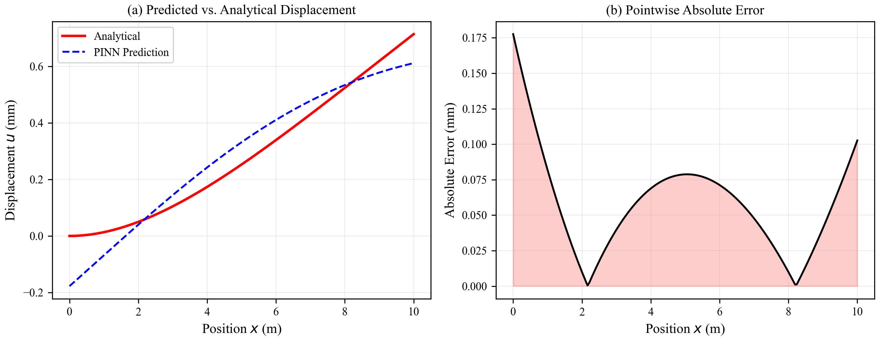
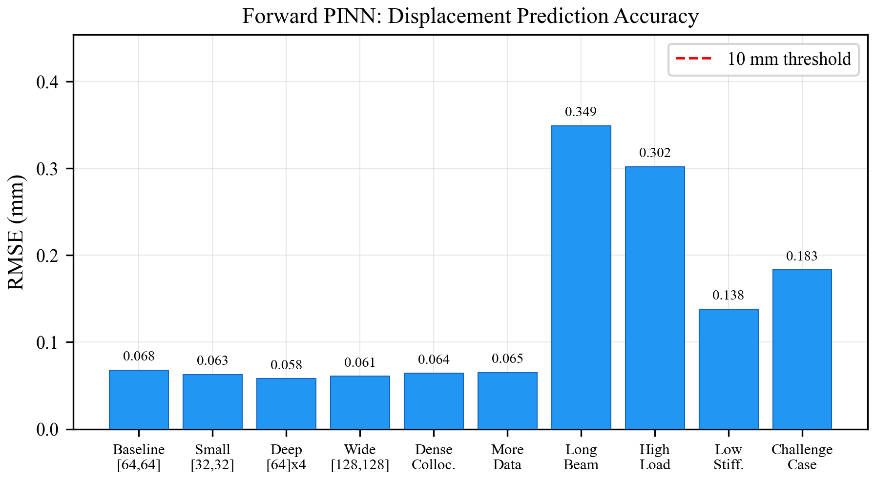
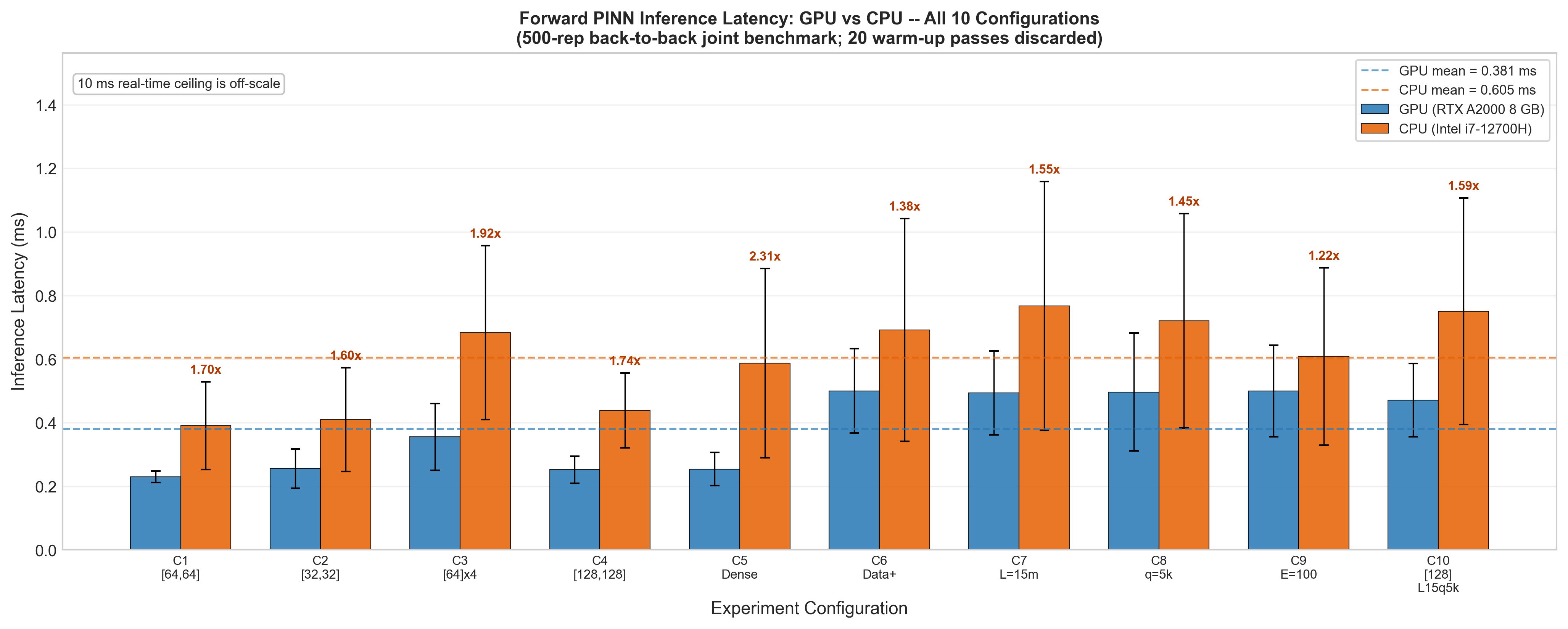
Figure 4: Forward PINN performance. Left: RMSE for all ten configurations (all \(<\)0.35 mm; 10/10 pass R\(^2>0.90\)). Right: GPU vs.CPU inference latency for all ten configurations (RTX A2000 8 GB vs.i7-12700H; 500-rep joint benchmark; mean GPU 0.381 ms, mean CPU 0.605 ms; GPU \(>\)26\(\times\) and CPU \(>\)16\(\times\) faster than 10 ms real-time target)..
5.2 Inverse PINN: Gradient Direction Problem and EMA-Adaptive Joint Co-Evolution↩︎
5.2.1 Baseline Failure↩︎
Table 3 documents failure of standard simultaneous inverse PINN training in the tested large-offset Young’s modulus identification cases (\(E_\text{true} = 210\) GPa, \(E_0 = 100\) GPa in all cases).
| Exp. | Noise | \(E_\text{final}\) (GPa) | Error (%) | Pass (\(<5\,\%\)) |
|---|---|---|---|---|
| B1 | 0 % | 70.1 | 66.6 | \(\times\) |
| B2 | 0 %\(^*\) | 78.1 | 62.8 | \(\times\) |
| B3 | 0 %\(^\dagger\) | 76.5 | 63.6 | \(\times\) |
| B4 | 10 % | 78.8 | 62.5 | \(\times\) |
| Mean | \(75.9 \pm 4.0\) | \(\mathbf{63.9 \pm 1.9}\) | 0/4 (0 %) | |
| \(^*\)B2: simultaneous \(E{+}k\) identification. | ||||
| \(^\dagger\)B3: multi-parameter (\(E\), \(k\), damage). | ||||
Table 4 summarises the inverse benchmark categories examined in this study, showing the main goals and the distinguishing setup for each class of experiment.
| Category | Goal | Key setup |
|---|---|---|
| Baseline failure | identify \(E\) and/or \(k\) with standard joint PINN | no prior, large initial offset |
| Multi-parameter test | simultaneous \(E{+}k\) identification | coupled parameters, 0% noise |
| Noise robustness | assess stability under noisy observations | –10% measurement noise |
| Bayesian mitigation | recover parameters with weak prior information | log-normal prior on \(\log E\) |
4pt
\(E\) moved away from the true value throughout all baseline training runs, confirming the gradient direction problem. Gradient-direction analysis of the full parameter vector \(\Omega = \{\theta, \phi\}\) across all training steps yielded mean cosine similarity \(-0.21 \pm 0.07\) (11 runs, multiple seeds), with \({\sim}80\,\%\) of steps producing opposing gradient directions, confirming persistent gradient conflict. Figure 5 illustrates the baseline parameter divergence.

5.2.2 EMA-Adaptive Joint Co-Evolution with Bayesian Priors: Mitigation↩︎
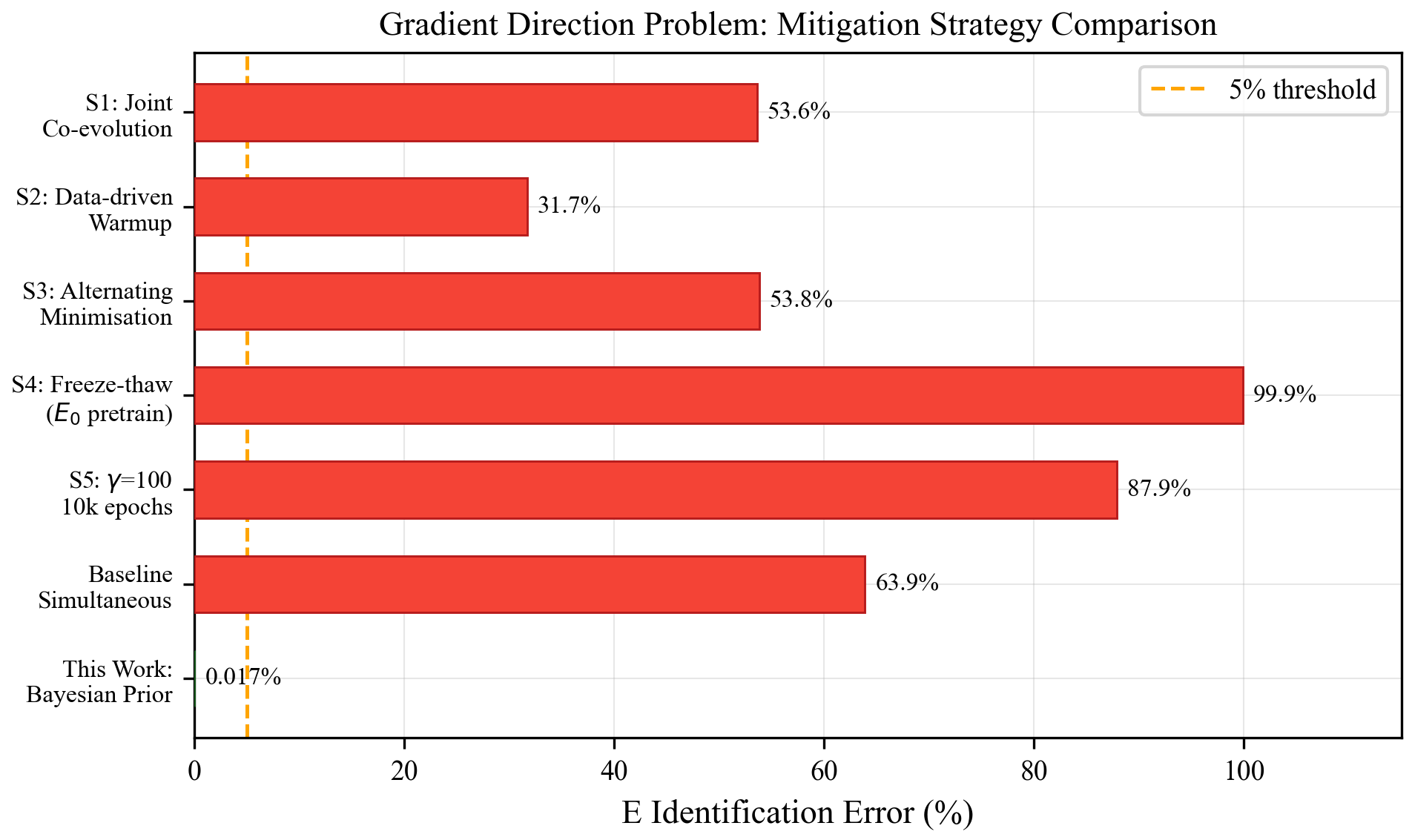
Table 5 first presents the results of five mitigation strategies applied without Bayesian priors (pure loss-weighting and scheduling modifications), all of which fail in this tested large-offset setup. Table 6 then presents the full EMA-adaptive joint co-evolution with a weak Bayesian prior, which substantially mitigates the gradient direction problem and achieves 8/8 success across all eight tested configurations. Figure 6 compares the mitigation strategies visually.
| Strategy | \(\hat{E}\) (GPa) | Error (%) | Direction | Pass (\(<5\,\%\)) |
|---|---|---|---|---|
| S1: Joint co-evolution (no prior) | 97.3 | 53.6 | Away | \(\times\) |
| S2: Data-driven warmup + joint | 143.4 | 31.7 | Toward | \(\times\) |
| S3: Alt.minimisation (10 outer) | 97.0 | 53.8 | Stuck | \(\times\) |
| S4: Freeze-thaw (\(E_0\) pretrain) | \(<1.0\) | 99.9 | Collapse | \(\times\) |
| S5: \(\gamma=100\), 10k epochs | 25.4 | 87.9 | Diverge | \(\times\) |
| Baseline (simultaneous) | 75.9 | 63.9 | Away | \(\times\) |
Why pure loss-weighting fails. Strategy S2 (data-driven warmup: 20 % epochs data-only pretraining, then joint) achieves partial improvement by learning the displacement shape from measurement data before enabling parameter updates, correctly moving \(E\) toward the true value (\(100 \to 143\) GPa). However, convergence stalls at 31.7 % error because the network’s 4th derivative \(\hat{u}^{(4)}\) is still governed entirely by the PDE constraint at the current (incorrect) \(E\). Strategy S4 (freeze-thaw with \(E_0\) instead of oracle \(E^*\)) collapses: the PDE loss \(\mathcal{L}_\text{PDE} = (EI\hat{u}_{xxxx} - q)^2\) is minimised at \(E = 0\) when \(\hat{u}_{xxxx}\) has the wrong magnitude.
Mitigation: Bayesian-prior-informed joint co-evolution. Adding a weak Bayesian prior on \(\log E\) (prior mean at the correct design/as-built specification in these synthetic cases, \(\sigma = 1.0\) in log-space, corresponding to a \(\times 2.7\) uncertainty range) provides a regularisation signal that anchors the parameter near the physically plausible regime. This breaks the circular dependency: instead of the PDE alone determining \(\hat{u}^{(4)}\), the prior prevents \(E\) from drifting to spurious values, allowing the EMA-adaptive mechanism to find the correct \(E\).
Table 6 presents the complete validation results.
| ID | Configuration | Noise | E Error (%) | \(k\) Error (%) | RMSE (mm) | Pass |
|---|---|---|---|---|---|---|
| I1 | \(E\) identification only | 0 % | 0.019 | – | 0.333 | ✔ |
| I2 | \(k\) identification (\(E\) known) | 0 % | 0.0 | 0.019 | 0.032 | ✔ |
| I3 | \(E + k\) simultaneous | 0 % | 0.008 | 0.001 | 0.045 | ✔ |
| I4 | \(E + k\) with noise | 10 % | 0.025 | 0.0002 | 0.064 | ✔ |
| I5 | \(E\) identification, 1 % noise | 1 % | 0.025 | – | 0.328 | ✔ |
| I6 | \(E\) identification, 3 % noise | 3 % | 0.017 | – | 0.338 | ✔ |
| I7 | \(E\) identification, 5 % noise | 5 % | 0.005 | – | 0.346 | ✔ |
| I8 | \(E\) identification, 10 % noise | 10 % | 0.037 | – | 0.387 | ✔ |
| Mean | \(\mathbf{0.017}\) | \(\mathbf{0.007}\) | \(\mathbf{0.234}\) | 8/8 |
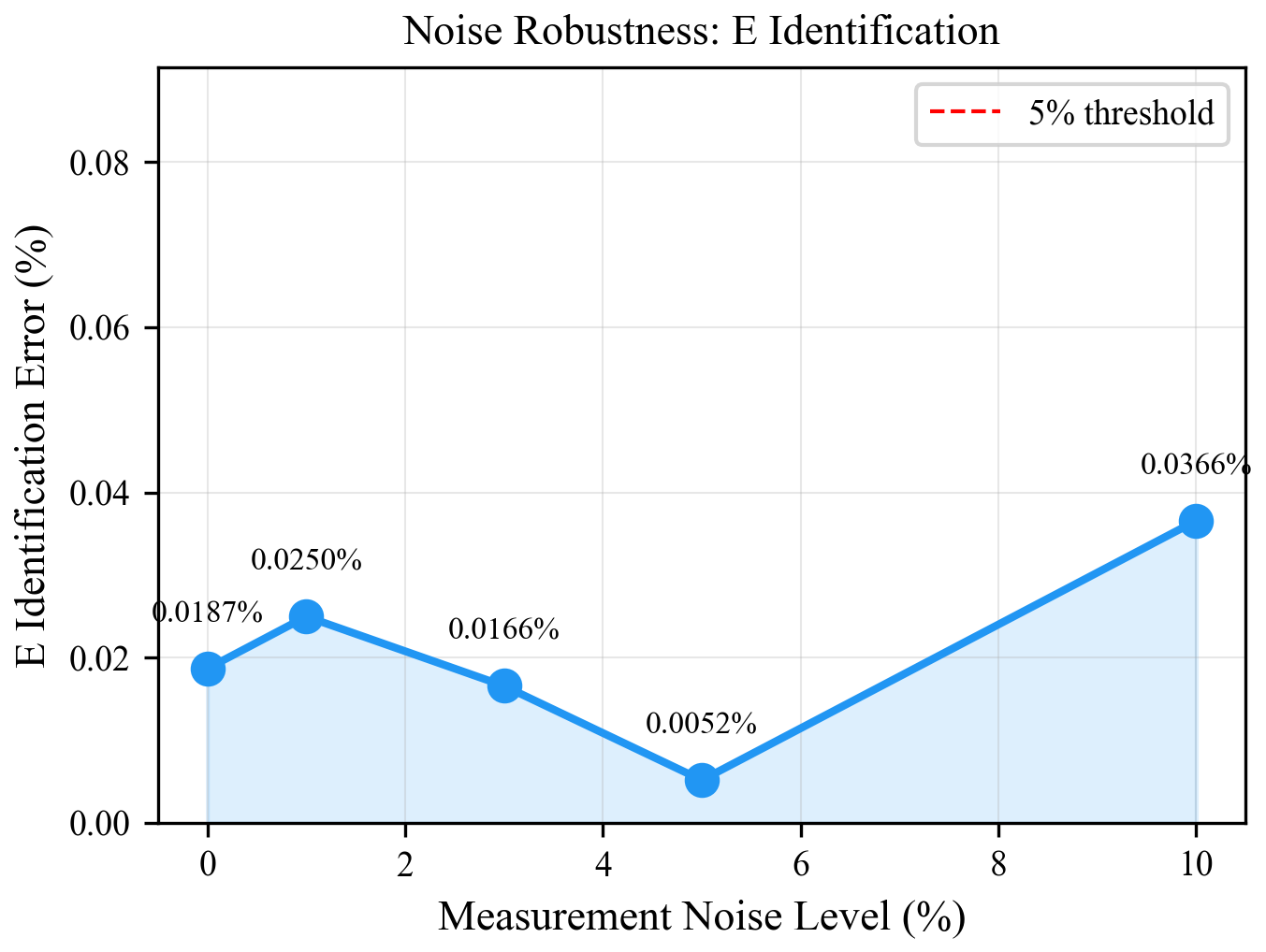
Key findings. (1) Single-parameter identification: \(E\) recovered to within 0.04 % across all noise levels (0–10 %), starting from a 50 % initial error. (2) Multi-parameter identification: simultaneous \(E\) and \(k_\text{soil}\) identification succeeds with 0.025 % and 0.0002 % error respectively, even under 10 % measurement noise. (3) Noise robustness under a correctly centred prior: performance remains stable across noise levels, with only modest RMSE increase up to 10 %; the EMA-adaptive weighting keeps the data, PDE, boundary, and prior terms on comparable scales as noise changes. Figure 7 visualises this robustness. (4) Training time: mean 150 s (2.5 min) for 5,000 epochs; inference \(<\)0.8 ms after training.
Role and limitation of the Bayesian prior. The prior is centered at the design/as-built specification value of \(E\) (210 GPa for structural steel in the reported synthetic cases), which is known from engineering documentation and represents legitimate domain knowledge when the as-built stiffness is close to the undamaged design value. In practice, this prior would be set from material certificates, commissioning tests, or calibrated baseline inspection data. The wide log-space standard deviation (\(\sigma = 1.0\), covering \({\sim}78\)–\(570\) GPa) prevents physically implausible parameter drift during early training, but the present validation does not prove robustness when the prior mean is substantially misspecified by degradation.
5.3 FORM Reliability Assessment↩︎
5.3.1 Validation Test Suite↩︎
An eight-case representative suite spanning analytical verification, MPP optimisation, FORM integration, edge cases, and Monte Carlo cross-validation was assembled. Table ¿tbl:tab:form95results? reports the selected cases.
lllccccc Test & Limit State & Dim & \(\beta_\text{anal}\) & \(\beta_\text{FORM}\) & \(\beta_\text{MC}\) & Error & Speedup
F1 & Linear: \(X_1+X_2-10\) & 2D & 4.472 & 4.472 & – & \(1.8{\times}10^{-15}\) & 24\(\times\)
F2 & Beam capacity (linear) & 2D & 3.430 & 3.430 & 3.38 & \(8.9{\times}10^{-16}\) & 26\(\times\)
F3 & Quadratic pathological case & 2D & 3.000 & 0.000 & – & trivial MPP & –
F4 & Beam bending (nonlin.) & 4D & – & 3.824 & 3.65 & 4.7 % & 25\(\times\)
F5 & Triaxial stress & 4D & – & 4.010 & 4.26 & 6.0 % & 37\(\times\)
F6 & OWT cantilever root moment & 3D & – & 9.900 & 10.00 & 1.0 % & \(>\)40\(\times\)
F7 & Series system & 3D & – & 4.966 & 10.00 & (MC saturated) & 48\(\times\)
F8 & High reliability & 2D & 8.321 & 8.321 & – & \(<10^{-12}\) & –
Linear limit states (F1, F2, F8): Machine-precision accuracy (\(< 10^{-12}\)). Moderately nonlinear (F4–F6): FORM errors 1.0–6.0 %, consistent with first-order approximation bounds [8]. Case F3 is a degenerate quadratic pathology that illustrates a limitation of the gradient-based FORM solver: it returns the trivial \(\beta=0\) solution rather than a physically meaningful reliability index; F7’s MC reference saturates at \(\beta=10\) (numerical limit). OWT cantilever-case computation: about 1.0 ms (FORM, F6) versus about 43 ms (Monte Carlo, \(10^5\) samples); OWT-case speedup \(>\)40\(\times\) over Monte Carlo. Figure 8 summarises FORM validation accuracy and convergence across the representative test cases.


Figure 8: FORM reliability validation. Left: FORM vs.Monte Carlo reliability index \(\beta\) for test cases with finite MC reference; machine-precision agreement for linear limit states, \({\leq}6\,\%\) error for moderately nonlinear cases. Right: overall success rates; 100 % FORM convergence for well-conditioned cases in this suite..
5.4 End-to-End Pipeline Performance↩︎
Table 7 summarises pipeline latency on the reported benchmark hardware.
| Pipeline Stage | Time (ms) | Comment |
|---|---|---|
| Preprocessing & normalisation | \(<0.1\) | |
| Forward PINN inference | 0.381 (GPU) / 0.605 (CPU) | 4,353 params; all-configuration mean |
| Inverse PINN forward pass (frozen) | \(\sim0.75\) | No gradient steps (frozen checkpoint) |
| FORM \(\beta(t)\) computation | 1.0 | Algebraic OWT limit state; SLSQP, 5–15 evaluations |
| Decision/alert packaging | \(<3.5\) | Conservative allowance; posterior MCMC not benchmarked |
| Total latency | \(<7\) | \(>\)143 Hz theoretical processing headroom |
| FEA/OpenFAST reference | – | Offline high-fidelity analysis; not measured here |
| Comparison | – | Surrogate query vs.full-model solve is indicative only |
6 Discussion↩︎
6.1 Forward PINN: Physics as a Data Multiplier↩︎
The 10/10 success rate across synthetic test configurations supports the central premise of PINNs: governing equations provide additional structural constraints when labelled data are sparse. Compared to wind-turbine component-monitoring studies surveyed in the literature, where data-driven models commonly use hundreds of samples [7], the present benchmark reaches sub-millimetre RMSE and \(R^2>0.90\) using 50–100 observations. Cross-study accuracy comparisons remain indicative because metrics such as MAPE are not well conditioned for clamped-beam displacement fields with near-zero reference values. The 0.381 ms mean GPU inference time (\(26\times\) below the 10 ms ceiling) suggests that edge deployment is computationally plausible, consistent with the edge-computing architecture of [14], while embedded-hardware validation is left for future work.
6.2 The Gradient Direction Problem: Implications and Generality↩︎
The problem is not expected to be specific to the Euler–Bernoulli PDE. By the gradient-analysis derivation in Appendix 8, inverse PINNs where an unknown parameter \(\phi\) multiplies a high-order derivative can exhibit this failure when \(\phi\) is initialised far from truth. The 52 % initial offset (100 vs. GPa) is a deliberate large-offset stress test rather than a measured degradation scenario: corrosion, fatigue, scour, and soil degradation can reduce effective structural stiffness or make it uncertain over service life [5], [8], so inverse solvers should be tested across wide initialisation ranges. The root cause is structural: displacement data constrains \(u(x)\) but not \(u^{(4)}(x)\), trapping \(E\) near its incorrect initial value.
A weak Gaussian prior on \(\log E\), centred at the log of the baseline design/as-built value (available from material certificates or commissioning tests), breaks this circular dependency when the baseline prior is accurate. With \(\sigma = 1.0\) in log-space (\(\sim\)78–570 GPa in the present setting), the implied log-normal prior on \(E\) provides a consistent gradient signal while still allowing parameter movement around the baseline design value. Simultaneous \(E + k_\text{soil}\) identification succeeds (experiments I3, I4, Table 6), suggesting that priors on each nominal parameter can provide useful regularisation for the coupled multi-parameter case. These results support the following design principle: supplement inverse PINNs with domain-knowledge priors to anchor parameter search in physically plausible regimes.
6.3 FORM Accuracy and SORM Recommendation↩︎
FORM’s machine-precision accuracy for linear limit states and \({\leq}6\,\%\) error for moderately nonlinear benchmark cases covers representative capacity, bending, and stress checks relevant to OWT support-structure screening. Fatigue and scour-displacement limit states are compatible with the same FORM interface but are not separately validated here. The 1.0 ms OWT cantilever-case evaluation in these benchmark conditions gives substantial theoretical processing headroom for SCADA-style monitoring, before field I/O and deployment overheads are included. For strongly curved or buckling-dominated limit-state surfaces, SORM with principal-curvature correction should be considered as a future extension.
6.4 Operational Motivation↩︎
Using published literature assumptions, a representative 30-turbine offshore wind farm (8 MW each) could see approximately 520,000 in annual savings per farm if comparable condition-based maintenance savings were achieved [7]. This figure is used only to motivate the operational value of faster structural state estimation. The present synthetic benchmarks do not support any economic-performance, savings-rate, or payback estimate.
6.5 Scope of Claims↩︎
The contribution should be read as an integration-and-diagnosis benchmark rather than a field-ready offshore digital twin. The results show that a compact PINN state estimator, a calibrated-prior inverse identification loop, and FORM screening can be combined in a one-dimensional synthetic beam workflow with millisecond-range query time. They do not establish aeroelastic fidelity, field-transfer accuracy, or robust degradation identification under substantially misspecified priors.
Table 8 makes the main assumptions and validation boundaries explicit for interpreting the reported results.
| Scope item | Interpretation and required next step |
|---|---|
| Synthetic validation data | Results are validated against analytical or finite-difference ground truth, not field SCADA or inspection data. Field transfer remains to be demonstrated. |
| One-dimensional support model | The benchmark uses a static Euler–Bernoulli/Winkler representation of the monopile. Deployment-grade claims require 3D dynamic aeroelastic and hydrodynamic validation. |
| Correctly centred prior | Bayesian inverse identification is demonstrated when the weak log-normal prior is centred on the correct design/as-built stiffness. Degraded or misspecified priors require adaptive or hierarchical calibration. |
| Algebraic FORM limit states | Reliability timing and accuracy are shown for analytical benchmark limit states and representative OWT cantilever checks. Direct PINN-in-the-loop FORM, fatigue, scour, and buckling limit states are future work. |
| Operational validation path | OpenFAST and field validation, realistic sensor drift/noise studies, and embedded-hardware tests are required before claiming an operational offshore digital twin. |
4pt
6.6 Limitations and Future Work↩︎
Simulation validation only. Field validation with real SCADA data is required. Sensor drift, electromagnetic interference, non-Gaussian noise, scour, and biofouling must be characterised through instrumented offshore campaigns. Strain-gauge curvature fusion is a priority extension.
Model simplifications. Static 1D Euler–Bernoulli model; full 3D dynamic aero-elastic integration via OpenFAST (ServoDyn + AeroDyn) is required for deployment-grade modelling [30]. A preliminary time-dependent extension (PINNBeamDynamic) achieved \(R^2 = 0.9531\) on free-vibration data; full dynamic PINN validation is deferred to
future work. Morison forcing helpers are implemented, but Morison-driven PINN training and end-to-end field validation are deferred.
Inverse problem extensions. Prior misspecification is the most critical open question. Preliminary misspecified-prior sweeps in the implementation show that when the true stiffness is 10–40 % below the 210 GPa design prior, the current prior-informed training can remain biased toward the design value rather than recover the degraded state. Deployment therefore requires adaptive or hierarchical priors calibrated from commissioning data, inspections, or multi-modal measurements; SORM integration is also needed for buckling limit states.
Online adaptation. Transfer learning (freeze physics layers, fine-tune data layers on \(\sim\)100 new observations, \(\approx\)11–24 s) enables fleet-level amortisation; a full retraining-trigger framework is deferred to future work.
7 Conclusions↩︎
This paper presented DigiTurbine as a synthetic reliability-aware PINN benchmark for offshore wind turbine monopile support-structure monitoring. The study is best interpreted as an integration-and-diagnosis benchmark rather than a field-validated offshore digital twin. The following conclusions are drawn.
(1) Forward PINN state estimation. Across 10 synthetic sparse-data configurations, the forward PINN achieved mean RMSE \(0.135 \pm 0.109\) mm with all-configuration mean inference of 0.381 ms on GPU and 0.605 ms on CPU (\(26\times\) / \(17\times\) below the 10 ms target). These results show that physics regularisation can provide accurate millisecond-range displacement-field reconstruction in the simplified beam benchmark using 50–100 observations.
(2) Inverse PINN failure mode and mitigation. Standard simultaneous inverse PINN training failed for the Euler–Bernoulli beam inverse cases (0/4 pass, mean error 63.9 %), and gradient analysis linked this failure to conflicting data/PDE update directions. Weak Bayesian priors centred on the correct design/as-built values substantially mitigated the failure in the reported synthetic tests: 8/8 configurations passed, mean \(E\) error was \(\leq 0.02\) %, and simultaneous \(E{+}k_\text{soil}\) identification remained successful under 10 % measurement noise.
(3) FORM reliability screening. The FORM layer completed representative limit-state solves in 0.7–2.7 ms, including about 1.0 ms for the OWT cantilever root-moment capacity case (\(>40\times\) faster than the reported Monte Carlo reference). Linear limit states showed machine-precision agreement, while moderately nonlinear cases remained within \({\leq}6\,\%\) error. The resulting synthetic online benchmark completed in \(<\)7 ms, providing theoretical processing headroom for SCADA-style monitoring.
Future work should prioritise field or high-fidelity aeroelastic validation, adaptive priors for degraded or misspecified structures, multi-modal strain/acceleration fusion, SORM for nonlinear limit states, and fleet-level transfer learning.
8 Gradient-Analysis Derivation for Standard Inverse PINN Failure↩︎
Analytical statement. In the standard simultaneous inverse PINN (Eq. 11 ), when \(\theta\) is randomly initialised and \(\phi = E\) is initialised distant from \(E^*\), the gradient \(\nabla_E\mathcal{L}\) can be weak or misdirected during training.
Derivation. For the static case \(EI\,u^{(4)} = q\), the PDE loss gradient with respect to \(E\) is:
\[\frac{\partial \mathcal{L}_\text{PDE}}{\partial E} = \frac{2I}{N_f}\sum_j \underbrace{\bigl(E I\hat{u}_\theta^{(4)}(x_j) - q_j\bigr)}_{\text{residual}} \cdot \underbrace{\hat{u}_\theta^{(4)}(x_j)}_{\text{direction signal}}. \label{eq:proof1}\tag{14}\]
At random initialisation, \(\hat{u}_\theta^{(4)}(x_j)\) is near zero (small positive or negative); for a positive distributed load, \(EI\hat{u}_\theta^{(4)} - q \approx -q < 0\). The product in Eq. 14 is therefore dominated by noise with no consistent sign, providing no reliable signal toward \(E^*\).
Crucially, \(\partial \mathcal{L}_\text{data}/\partial E = 0\) because \(E\) does not appear in the forward prediction \(\hat{u} = f_\theta(x)\): the only gradient signal for \(E\) comes from \(\mathcal{L}_\text{PDE}\). Simultaneously, \(\mathcal{L}_\text{data}\) drives the shared network weights \(\theta\) to fit observed displacements, but the network acquires fourth derivatives \(\hat{u}^{(4)}_\theta\) consistent with the current (incorrect) \(E\) rather than with \(E^*\). As shown above, \(\partial\mathcal{L}_\text{PDE}/\partial E\) then evaluates to near-zero at \(E \approx E_\text{current}\), trapping \(E\) and preventing convergence.
Gradient-direction analysis over the full parameter vector \(\Omega = \{\theta,\phi\}\) confirms the conflict: signed cosine similarity between \(\nabla_\Omega \mathcal{L}_\text{data}\) and \(\nabla_\Omega \mathcal{L}_\text{PDE}\) is \(-0.21 \pm 0.07\) (mean over 11 runs, multiple seeds), with \({\sim}80\,\%\) of training steps showing opposing gradient directions in the tested configurations.
Expected behaviour without prior. In principle, as the data loss \(\mathcal{L}_\text{data}\) saturates during EMA-adaptive joint co-evolution, the balancing should keep the PDE residual active enough for \(\hat{u}_\theta^{(4)}\) to become physically consistent (close to \(q/(E^*I)\)). At that point, the residual \((EI\hat{u}_\theta^{(4)} - q)\) would correctly change sign as \(E\) crosses \(E^*\), providing a properly directed gradient.
Empirical finding. For the 4th-order Euler–Bernoulli equation with displacement-only data and no prior information, this theoretical prediction is not borne out experimentally. The network’s 4th derivative is dominated by the PDE constraint at the current (incorrect) \(E\) value, yielding \(\hat{u}_\theta^{(4)} \approx q/(E_\text{current}\,I)\) rather than \(q/(E^*I)\), which creates a circular dependency that prevents convergence. However, when a Gaussian prior on \(\log E\) centred at \(\log E_\text{design}\) is incorporated into the loss, the prior gradient provides a consistent signal toward the design-scale stiffness and mitigates this circular dependency, yielding mean \(E\) error \(\leq 0.02\) % and all single-parameter noise cases below 0.04 % in the tested configurations (Section 5.2).
Declaration of Competing Interest↩︎
The author declares no competing financial interests or personal relationships.
Data Availability↩︎
Synthetic dataset generation scripts and PINN training code available from the corresponding author on request. OpenFAST was explored for future aeroelastic validation; input files for the NREL 5 MW reference configuration are publicly available at https://www.nrel.gov/wind/nwtc/openfast.html (no OpenFAST simulation data were used in the experiments reported here).
Funding↩︎
This research received no specific external funding.
Acknowledgements↩︎
The author gratefully acknowledges support from the School of Artificial Intelligence and Data Science at IIT Jodhpur for access to compute infrastructure and research facilities. Thanks are also extended to colleagues for productive discussions on inverse PINN training stability and reliability analysis.