Public Good Provision under Locally Private Signals
June 22, 2026
Abstract
We study public-good provision when a planner observes agents’ preferences only through a fixed local-privacy channel that randomizes each report before it reaches the planner. We characterize the optimal reduced-form allocation: the project is implemented when an aggregate posterior score is positive, where each agent’s score combines the posterior expected valuation and posterior virtual value. Privacy enters through these posterior objects, muting the responsiveness of provision to private preferences and, under weak monotone likelihood ratios, potentially generating pooling. We then distinguish the optimal reduced-form allocation from its implementation through signal-measurable transfers: the required transfers solve a Fredholm integral equation whose solution is unique under completeness when it exists, while existence requires a separate range condition. Maximum reduced-form revenue exhibits three population regimes: it is asymptotically linear, of square-root order, or exponentially small according as the lower endpoint of the valuation distribution is positive, zero, or negative. Finally, welfare comparisons depend on the privacy calibration. At a common noise scale, Laplace Blackwell-dominates logistic noise, while under a common tight \(\mu\)-GDP calibration the ordering reverses for the maximally separated binary endpoint experiment. Thus the preferred privacy channel depends on the standard used to hold privacy fixed.
Keywords: local differential privacy; mechanism design; public-good provision; Myerson virtual values; large deviations.
JEL classification: D82, D44, C72, H41.
Credit authorship contribution statement:
Behrooz Moosavi: Review & editing, Writing original draft, Methodology, Investigation, Conceptualization.
Jordan Awan: Review & editing, Writing original draft, Methodology, Investigation, Conceptualization.
Conflict of Interest: The authors declare that they have no conflict of interest.
Funding: This work was supported in part by NSF award number SES-2610910.
1 Introduction↩︎
Classical mechanism design relies on the sensitivity of outcomes to individual reports. Vickrey–Clarke–Groves payments [1]–[3] charge each agent the externality it imposes on the others; the Myerson envelope theorem [4] recovers information rents from the interim allocation rule, since an agent’s equilibrium utility has derivative equal to its allocation probability and rents are the integral of that allocation over types. Differential privacy demands the opposite: the distribution of a released output must change only slightly when any single input changes [5], [6]. Local differential privacy enforces this by randomizing each input before it reaches the collector.
This architecture is already deployed at the scale of the world’s largest data collectors. Apple has used local differential privacy in iOS to gather usage statistics from hundreds of millions of devices, with randomization performed on the user’s device before any data reaches its servers [7], [8], and Google’s RAPPOR system applied the same local model in Chrome [9]. In both, the collector is untrusted and observes only a randomized signal, never the true input. These systems perform statistical estimation, with no transfers, incentive constraints, or collective decision at stake; the conflict with mechanism design arises only when such a channel is placed in front of a planner who must elicit preferences, make a public decision, and raise revenue from privatized signals alone. There, neither the standard allocation rule nor the standard payment identity survives unchanged.
This paper characterizes the optimal reduced-form mechanism and the asymptotic behavior of maximum reduced-form revenue in such an environment. A planner must decide whether to implement a binary public project—build or not build—when \(n\) agents hold privately known valuations \(X_1,\ldots,X_n\). The planner does not observe these valuations. Each agent submits a value to a fixed trusted mediator (privacy channel), which randomizes the submission before transmitting it to the planner; the agent controls the value it submits but neither observes nor controls the realized noise, and cannot bypass the protocol. The planner observes only the privatized signal profile \((Y_1,\ldots,Y_n)\), so both the project decision and the transfer schedule must be measurable functions of these signals alone. The mechanism must be Bayesian incentive compatible, so that truthful submission is optimal for every type; we analyze the resulting truthful equilibrium, along which the submitted value equals the valuation and the privatized signal is distributed as \[Y_i\sim K(\,\cdot\mid X_i).\] It must also be individually rational and meet an ex-ante revenue target.
This formulation fits settings in which preference-relevant information is generated or measured locally and passed through a prescribed privacy device before reaching an untrusted aggregator: federated rollout decisions based on privatized quality or demand reports, consortium or standard-adoption decisions in which members privatize their preferences from the aggregator, and more generally any binary collective decision mediated by a fixed local randomization protocol. Within this class we ask three questions. How strong can the privacy guarantee become before the project can no longer be financed, and how does this relate to the classical difficulty of public-good provision with many privately informed agents [10]? What form does the optimal decision rule take when the planner observes only privatized signals? And, once channels are calibrated to a common privacy benchmark, does the choice of noise distribution—Gaussian, Laplace, or logistic—affect welfare and revenue, or only the statistical precision of the planner’s information?
1.0.0.1 Our Contributions.
This paper makes four contributions.
Privacy reshapes how the good is provided. The planner never sees agents’ true values, only reports passed through a fixed, privacy-protecting noise channel. We show that the planner should nonetheless act on a simple per-agent index that blends how much each agent is expected to value the good with how much revenue can be collected from them, and should provide the good when these indices sum to a positive total. The amount of noise the channel adds controls how strongly provision responds to people’s underlying preferences; coarser channels can leave the planner unable to tell apart agents whose reports are extreme.
Knowing what to provide is not the same as being able to pay for it. We distinguish the allocation the planner would choose from the payments needed to make truth-telling optimal. Recovering payments that depend only on the noisy reports is a separate and harder problem—formally, solving an integral (Fredholm) equation—that may have no exact solution. When an exact solution exists it is unique, but existence is not automatic. The Online Supplement therefore also constructs payments that work approximately, with explicit bounds on how far incentives, participation, and revenue can be off.
Privacy makes public goods harder to finance as the market grows. The revenue a privacy-respecting mechanism can raise is governed by the lower endpoint of the valuation distribution—the smallest value an agent could have. As the number of agents grows, revenue grows in proportion to the market when that lower endpoint is positive, grows only at a slow square-root rate when it is exactly zero, and shrinks to almost nothing when it is negative. The change between a fundable and an unfundable good is sharp, so a small tightening of the revenue requirement can switch provision off.
The better privacy technology depends on how privacy is measured. Comparing two natural noise designs, Laplace and logistic, we find no design is better in every case. Holding the noise scale fixed—a common pure-\(\epsilon\) calibration—the Laplace design gives the planner more usable information; holding fixed instead a stricter hypothesis-testing privacy standard (Gaussian differential privacy), the ranking reverses in the hardest case, that of telling apart the highest- and lowest-value agents. Which design a planner prefers thus depends on the privacy standard used to compare them, and this reversal does not extend to a blanket ranking across all agents.
1.0.0.2 Related literature.
Our work lies at the intersection of differential privacy, mechanism design, and public-good provision. The privacy-aware mechanism-design literature begins with [11], who use the stability created by differential privacy to obtain approximate truthfulness. We study a different problem: the local privacy channel is fixed exogenously, privacy does not enter agents’ payoffs, and the planner must achieve exact Bayesian incentive compatibility using allocation and transfer rules that depend only on privatized signals. The classical transfer identity [4] therefore becomes an inverse problem: recovering a signal-contingent transfer requires solving a Fredholm equation of the first kind, where completeness of the channel kernel gives uniqueness when a solution exists and existence is a separate range condition. Recent work also studies privacy-constrained mechanism and information design: [12] incorporate belief-based privacy costs into mechanism design and show that privacy concerns can rationalize coarse mechanisms, while [13] characterize signals that conceal a protected attribute through garbling and mean-preserving contraction and [14] study signals that reveal information about a common state without revealing other agents’ signals. We share their use of garbling and the Blackwell order, but our planner does not design the information structure: it faces a fixed local differential-privacy channel and optimizes a public-good mechanism conditional on the information that channel produces. Two further strands bear on our setting and are developed in the Online Supplement: privacy as a payoff argument or a good to be compensated [15]–[17], and the statistical limits of local privacy [18], [19], where our concern is the privacy–revenue rather than the privacy–estimation frontier.
The paper most closely related to ours is [20], who study binary public-good provision with \(\pm1\) types transmitted through a randomized-response flip channel. They characterize Boolean decision rules trading off revenue, surplus, and noise sensitivity. We allow continuous valuations and a broader class of channels, so monotone likelihood ratios govern implementability and generate features without a Boolean analogue, including the distinction between strict and weak MLRP and Laplace tail pooling. We also characterize transfers through a Fredholm equation, allow a hierarchical prior, and derive three large-population revenue regimes—linear, square-root, and exponentially small—according to the sign of the lower endpoint of the valuation distribution.
Finally, our asymptotic analysis relates to the literature on public-good provision in large economies [10], [21], [22], where private information obstructs efficient provision and, under budget balance, the obstruction intensifies as the population grows. [23] identify a square-root boundary in the growth rate of project costs for asymptotically efficient provision. Their boundary concerns cost scaling and is therefore analogous to, but distinct from, our knife-edge regime, in which maximal reduced-form revenue is itself of square-root order. In our model the local privacy channel further determines the speed at which revenue feasibility deteriorates. The hierarchical extension is also related to [24]: a common latent parameter generates dependence across types, while privacy weakens the information each signal conveys about that parameter without eliminating the induced correlation.
1.0.0.3 Outline
The paper is organized as follows. Section 2 reviews the public-good problem and the privacy channels; Section 3 sets up the mediated reporting model and the posterior-score objects it relies on. Section 4 gives the main results: the optimal threshold rule, the Fredholm implementation problem, the linear/square-root/exponential revenue regimes, the hierarchical extension, and the channel welfare reversal. Section 5 illustrates some of the theoretical results derived in section 4. The appendices collect the proofs and additional numerical results, and the online supplement develops exact and approximate signal-measurable implementation, the revelation and completeness arguments, and the full numerical methodology.
2 Background↩︎
This section sets out the economic environment, the reporting and privacy architecture, and the privacy criteria. The planner’s mechanism-design problem is formulated in Section 3. Trade-off functions, privacy calibrations, and channel-specific likelihood-ratio calculations are collected in Appendix 7.
2.1 Agents and Preferences↩︎
A planner faces \(n\) agents indexed by \(i\in\{1,\ldots,n\}\). Agent \(i\) privately observes a valuation \[X_i\in\mathcal{X}=[\underline{x},\bar{x}]\subset\mathbb{R}.\] In the known-prior benchmark, the valuations are independently and identically distributed according to a commonly known distribution \(F\) with density \(f>0\) on \(\mathcal{X}\).
The planner decides whether to implement a binary public project, \(q\in\{0,1\}\), and assigns transfers \(t_i\in\mathbb{R}\). Preferences are quasilinear: \[\label{eq:utility} u_i(q,t_i\mid x_i) = q\,x_i-t_i.\tag{1}\] The valuation \(x_i\) is the net value of implementation, inclusive of any exogenously assigned cost share. If the planner observed the valuation profile \(x=(x_1,\ldots,x_n)\), the efficient allocation would be \[\label{eq:first95best} q^{\mathrm{FB}}(x) = \mathbf{1}\!\left\{ \sum_{i=1}^{n}x_i\ge0 \right\}.\tag{2}\]
Example 1 (Shared community project). Suppose households decide whether to build a shared facility, such as a community solar array. The value \(x_i\) is household \(i\)’s benefit net of its assigned cost share. Thus \(x_i>0\) for a net beneficiary and \(x_i<0\) for a net payer, while \(\underline{x}<0\) permits some households to be net losers. The decision \(q=1\) means that the project is built, and \(t_i\) is the fee charged to household \(i\). By 2 , the efficient rule builds exactly when aggregate net value is nonnegative. The planner does not observe these valuations directly, which motivates the privacy channel below.
2.2 Strategic Reports and the Privacy Channel↩︎
After observing \(X_i=x_i\), agent \(i\) submits a report \(R_i=r_i\in\mathcal{X}\) to a trusted local mediator. Conditional on the report, the mediator generates a privatized signal through a fixed Markov kernel: \[\label{eq:channel} Y_i\mid R_i=r_i \sim K(\cdot\mid r_i).\tag{3}\] When the kernel admits a density, it is denoted by \(k(y_i\mid r_i)\). Signals take values in a measurable space \(\mathcal{Y}\subseteq\mathbb{R}\), with \(\mathcal{Y}=\mathbb{R}\) for the additive channels considered below.
The agent controls the report entering the channel but not the realized channel noise. The planner observes only the signal profile \[Y=(Y_1,\ldots,Y_n)\] and observes neither \(X\) nor \(R\).
A randomized signal-measurable mechanism is a measurable map \[\label{eq:mechanism95def} (q,t): \mathcal{Y}^n \longrightarrow [0,1]\times\mathbb{R}^n, \qquad y \longmapsto \bigl(q(y),t_1(y),\ldots,t_n(y)\bigr),\tag{4}\] where \(q(y)\) is the probability of implementation and \(t_i(y)\) is agent \(i\)’s payment. Transfers are assumed measurable and integrable under the induced signal laws. The realized project decision is binary; \(q(y)\in[0,1]\) denotes its implementation probability conditional on the signal profile.
We study direct reporting mechanisms, in which the value an agent submits is itself the input to the fixed privacy channel. Bayesian incentive compatibility, imposed in Section 3.1, requires truthful reporting \(R_i=X_i\) to be optimal within this reporting game. Along the resulting truthful equilibrium path, \[\label{eq:truthful95signal95law} Y_i\mid X_i=x_i \sim K(\cdot\mid x_i).\tag{5}\] The report variable is retained to formulate deviations, whereas posterior beliefs, welfare, revenue, and allocation are evaluated under the truthful law 5 .
Conditional independence of the mediator’s randomizations gives \[\label{eq:truthful95joint95channel} Y\mid X=x \sim \prod_{i=1}^{n}K(\cdot\mid x_i).\tag{6}\] The truthful-path marginal density of one signal is3 \[\label{eq:marginal95signal95density} m(y) = \int_{\mathcal{X}}k(y\mid x)f(x)\,dx.\tag{7}\] Under the independent known-prior benchmark, \[\label{eq:joint95signal95density} f_Y(y) = \prod_{i=1}^{n}m(y_i), \qquad f_{Y_{-i}}(y_{-i}) = \prod_{j\ne i}m(y_j).\tag{8}\]
2.3 Privacy Criteria↩︎
Privacy is measured through hypothesis-testing trade-off functions, with Gaussian differential privacy providing the common cross-family benchmark [25]. For probability measures \(P\) and \(Q\) on a common measurable signal space, define \[\label{eq:tradeoff95function} \mathcal{T}(P,Q)(\alpha) = \inf_{\psi} \left\{ 1-\mathbb{E}_Q[\psi]: \mathbb{E}_P[\psi]\le\alpha \right\}, \qquad \alpha\in[0,1],\tag{9}\] where the infimum is over measurable randomized tests \(\psi:\mathcal{Y}\to[0,1]\). Thus, \(\mathcal{T}(P,Q)(\alpha)\) is the smallest attainable type-II error among tests whose type-I error is at most \(\alpha\). A larger trade-off function corresponds to a less informative binary experiment and therefore stronger hypothesis-testing privacy.
Definition 1 (\(\mu\)-Gaussian local differential privacy). For \(\mu\ge0\), define \[\label{eq:gaussian95tradeoff} G_\mu(\alpha) = \Phi\!\left( \Phi^{-1}(1-\alpha)-\mu \right), \qquad \alpha\in[0,1].\tag{10}\] A channel \(K\) satisfies \(\mu\)-Gaussian local differential privacy, abbreviated \(\mu\)-GDP, if \[\label{eq:gdp} \mathcal{T}\!\left( K(\cdot\mid r), K(\cdot\mid r') \right)(\alpha) \ge G_\mu(\alpha)\tag{11}\] for every \(r,r'\in\mathcal{X}\) and every \(\alpha\in[0,1]\).
Smaller values of \(\mu\) correspond to stronger privacy. The Gaussian shift experiment \[\mathcal{N}(0,1) \quad\text{versus}\quad \mathcal{N}(\mu,1)\] has trade-off function \(G_\mu\).
Definition 2 (Approximate local differential privacy). For \(\epsilon\ge0\) and \(\delta\in[0,1]\), a channel \(K\) satisfies \((\epsilon,\delta)\)-local differential privacy if \[\label{eq:approx95ldp} K(S\mid r) \le e^\epsilon K(S\mid r') + \delta\tag{12}\] for every \(r,r'\in\mathcal{X}\) and every measurable \(S\subseteq\mathcal{Y}\).
The parameter \(\epsilon\) bounds multiplicative distinguishability, while \(\delta\) allows an additive exceptional probability [5], [6]. A \(\mu\)-GDP channel satisfies \((\epsilon,\delta_\mu(\epsilon))\)-LDP for every \(\epsilon\ge0\), where \[\label{eq:gdp95to95approx} \delta_\mu(\epsilon) = \Phi\!\left( -\frac{\epsilon}{\mu}+\frac{\mu}{2} \right) - e^\epsilon \Phi\!\left( -\frac{\epsilon}{\mu}-\frac{\mu}{2} \right)\tag{13}\] [25].
Remark 1 (Pure local differential privacy). Pure \(\epsilon\)-LDP is the case \(\delta=0\): \[\label{eq:pure95ldp} K(S\mid r) \le e^\epsilon K(S\mid r') \qquad \forall r,r'\in\mathcal{X}, \quad \forall\text{ measurable }S\subseteq\mathcal{Y}.\tag{14}\] When conditional densities exist, this is equivalent to \[\label{eq:pure95ldp95density} k(y\mid r) \le e^\epsilon k(y\mid r') \qquad \text{for a.e. }y, \quad \forall r,r'\in\mathcal{X}\tag{15}\] [26].
Pure LDP, approximate LDP, and GDP are distinct restrictions. Equal values of \(\epsilon\), equal noise variances, or equal noise scales do not generally equalize the complete testing trade-off functions of different channel families.
2.4 Channel Families↩︎
We study additive location channels of the form \[\label{eq:additive95channel} Y_i = R_i+\eta_i,\tag{16}\] where the noise variables are independent across agents and independent of \((X,R)\). Since reports lie in \([\underline{x},\bar{x}]\), the largest separation between any two reports is the type-space width \[\label{eq:type95sensitivity} \Delta_{\mathcal{X}} = \bar{x}-\underline{x},\tag{17}\] which plays the role of the sensitivity in the privacy calibrations below.
| Channel | Signal model | Conditional density | Standard calibration | ||||||
|---|---|---|---|---|---|---|---|---|---|
| Gaussian | \(Y_i^{G}=R_i+\eta_i^{G}\) \(\eta_i^{G}\sim\Normal(0,\sigma^2)\) |
\(\dfrac{1}{\sigma}\, \varphiN\!\left(\dfrac{y-r}{\sigma}\right)\) | Exact \(\mu_G(\sigma)\)-GDP, \(\mu_G(\sigma)=\Delta_{\X}/\sigma\); no finite pure \(\epsilon\) |
||||||
| Laplace | \(Y_i^{L}=R_i+\eta_i^{L}\) \(\eta_i^{L}\sim\Lap(0,b_L)\) |
\(\dfrac{1}{2b_L}e^{-|y-r|/b_L}\) | Pure \(\epsilon\)-LDP, \(b_L=\Delta_{\X}/\epsilon\) |
||||||
| Logistic | \(Y_i^{\mathrm{Log}}=R_i+\eta_i^{\mathrm{Log}}\) \(\eta_i^{\mathrm{Log}}\sim\Logistic(0,\beta)\) |
\(\dfrac{e^{-(y-r)/\beta}}{\beta[1+e^{-(y-r)/\beta}]^2}\) | Pure \(\epsilon\)-LDP, \(\beta=\Delta_{\X}/\epsilon\) |
6pt
Along the truthful path, \[\label{eq:truthful95channel95summary} Y_i^{G} = X_i+\eta_i^{G}, \qquad Y_i^{L} = X_i+\eta_i^{L}, \qquad Y_i^{\mathrm{Log}} = X_i+\eta_i^{\mathrm{Log}}.\tag{18}\]
Privacy limits the distinguishability of reports. The monotone likelihood ratio property introduced in Section 3.2 is a distinct property: it governs how signals order posterior beliefs and therefore how the mechanism responds to signal realizations.
3 Setup↩︎
This section formulates the planner’s problem, states the maintained assumptions, and records the reduced-form identities used in Section 4. General incentive, integrability, posterior, and monotonicity arguments are collected in Appendix 8; mechanism-specific proofs are collected in Appendix 9.
3.1 The Planner’s Problem↩︎
Figure 1 summarizes the timing. Agent \(i\) observes \(X_i\), submits \(R_i\), the mediator draws \(Y_i\sim K(\cdot\mid R_i)\), and the planner chooses \(q(Y)\) and \(t(Y)\).
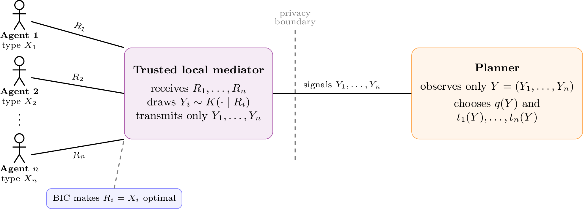
For a signal-measurable mechanism, define agent \(i\)’s interim allocation and interim payment after report \(r_i\), holding the other agents to truthful reporting, by \[\begin{align} Q_i(r_i) &= \int_{\mathcal{Y}^n} q(y)\, k(y_i\mid r_i)\, f_{Y_{-i}}(y_{-i})\,dy, \tag{19} \\ T_i(r_i) &= \int_{\mathcal{Y}^n} t_i(y)\, k(y_i\mid r_i)\, f_{Y_{-i}}(y_{-i})\,dy. \tag{20} \end{align}\] A type \(x_i\) reporting \(r_i\) obtains \[\label{eq:deviation95utility} U_i(x_i,r_i) = x_iQ_i(r_i)-T_i(r_i),\tag{21}\] and truthful interim utility is \[\label{eq:truthful95interim95utility} U_i(x_i) = U_i(x_i,x_i) = x_iQ_i(x_i)-T_i(x_i).\tag{22}\]
The planner maximizes expected surplus subject to incentive, participation, and revenue constraints: \[\tag{23} \begin{align} \sup_{q,t}\quad & \mathbb{E}\!\left[ q(Y)\sum_{i=1}^{n}X_i \right] \notag \\ \text{subject to}\quad & x_iQ_i(x_i)-T_i(x_i) \ge x_iQ_i(r_i)-T_i(r_i), && \forall x_i,r_i\in\mathcal{X}, \tag{24} \\ & U_i(x_i)\ge0, && \forall x_i\in\mathcal{X}, \tag{25} \\ & \mathbb{E}\!\left[ \sum_{i=1}^{n}t_i(Y) \right] = \sum_{i=1}^{n}\mathbb{E}[T_i(X_i)] \ge R, && \tag{26} \\ & q:\mathcal{Y}^n\to[0,1], \qquad t_i:\mathcal{Y}^n\to\mathbb{R} \text{ measurable and integrable.} && \notag \end{align}\] The constraints are Bayesian incentive compatibility, interim individual rationality, and an ex-ante revenue requirement. The case \(R=0\) imposes expected non-deficit [4], [27].
3.2 Structural Assumptions↩︎
Assumption 1 (Regularity). The distribution \(F\) is absolutely continuous on \(\mathcal{X}=[\underline{x},\bar{x}]\), with continuously differentiable density \(f>0\). The virtual value \[\label{eq:virtual95value} J(x) = x-\frac{1-F(x)}{f(x)}\tag{27}\] is weakly increasing.
This is the standard one-dimensional regularity condition [4]. Log-concavity of \(1-F\) is sufficient [28].
Assumption 2 (Monotone likelihood ratio property). The kernel has a strictly positive density \(k(y\mid x)\) on a common support \(\mathcal{Y}\), and for every \(x_2>x_1\), \[\label{eq:mlrp} y \longmapsto \frac{k(y\mid x_2)}{k(y\mid x_1)}\tag{28}\] is weakly increasing.
Remark 2 (Strict and weak MLRP). Strict MLRP requires the likelihood ratio in 28 to be strictly increasing, whereas weak MLRP permits flat regions. Posterior expectations of increasing functions are weakly increasing under MLRP and strictly increasing under strict MLRP under the corresponding nondegeneracy conditions [29].
The Gaussian and logistic location channels satisfy strict MLRP. The Laplace location channel satisfies weak MLRP because its likelihood ratio is constant in both outer tails. On a bounded type space, this produces exact posterior pooling in the global signal tails. The resulting posterior score remains weakly increasing, so the allocation threshold remains monotone; flat regions generate pooling or ties rather than requiring ironing. The general argument is given in Lemma 10 and Remark 14 of Appendix 8. The channel-specific calculations are in Appendix 7.
Assumption 3 (Statistical completeness and transfer space). Let \[\mathcal{H} \subseteq L^1\!\bigl(\mathcal{Y},m(y)\,dy\bigr)\] be a Banach space of admissible opponent-averaged transfers. Suppose that there exists \(C_{\mathcal{H}}<\infty\) such that \[\label{eq:transfer95space95domination} \sup_{x\in\mathcal{X}} \int_{\mathcal{Y}} |g(y)|k(y\mid x)\,dy \le C_{\mathcal{H}}\|g\|_{\mathcal{H}} \qquad \forall g\in\mathcal{H}.\tag{29}\] Suppose further that bounded truncations of every \(g\in\mathcal{H}\) belong to \(\mathcal{H}\) and converge to \(g\) in the \(\mathcal{H}\)-norm.
If \(g\in\mathcal{H}\) satisfies \[\label{eq:completeness} \int_{\mathcal{Y}} g(y)k(y\mid x)\,dy = 0 \qquad \forall x\in\mathcal{X},\tag{30}\] then \[g=0 \qquad m(y)\,dy\text{-almost everywhere}.\]
The domination condition 29 makes the conditional-expectation operator bounded on the maintained transfer space, while completeness 30 makes that operator injective. These are distinct properties. Boundedness guarantees that the operator is well defined and continuous; completeness identifies the opponent-averaged transfer whenever an implementation exists. Neither property implies that the desired interim payment belongs to the range of the operator, so existence remains a separate range condition.
Assumption 3 is used only for signal-measurable transfer implementation. It is not required for the reduced-form allocation or revenue characterizations. Completeness is maintained here as a high-level condition on the chosen transfer space \(\mathcal{H}\); verifying it for particular channel families and function spaces is a separate operator-specific question.
Assumption 4 (Compactness and kernel continuity). The type space \(\mathcal{X}=[\underline{x},\bar{x}]\) is compact, \(\mathcal{Y}\subseteq\mathbb{R}\) is Borel, and the kernel has a jointly measurable density satisfying \[\label{eq:l195kernel95continuity} \lim_{x'\to x} \int_{\mathcal{Y}} \left| k(y\mid x')-k(y\mid x) \right|\,dy = 0 \qquad \forall x\in\mathcal{X}.\tag{31}\] Allocations satisfy \(0\le q\le1\), transfers are integrable under every admissible report profile, and the feasible set is nonempty.
The signal space may be unbounded. The continuity and Fubini–Tonelli consequences of this assumption are collected in Appendix 8. Additional boundedness and strict-feasibility conditions used only for existence and multiplier arguments are stated in Appendix 9.
3.3 Interim Reduction and Posterior Objects↩︎
Although the privacy channel changes the mapping from reports to the planner’s observations, each agent’s deviation problem remains one-dimensional. By 21 , a type \(x_i\) that reports \(r_i\) obtains \[x_iQ_i(r_i)-T_i(r_i),\] which is the standard one-dimensional screening payoff associated with interim allocation \(Q_i\) and interim payment \(T_i\).
Bayesian incentive compatibility is therefore equivalent to weak monotonicity of \(Q_i\) together with the envelope identity \[\label{eq:envelope} U_i(x_i) = U_i(\underline{x}) + \int_{\underline{x}}^{x_i}Q_i(z)\,dz,\tag{32}\] or, equivalently, \[\label{eq:transfer95identity} T_i(x_i) = x_iQ_i(x_i) - \int_{\underline{x}}^{x_i}Q_i(z)\,dz - U_i(\underline{x}).\tag{33}\] Since \(Q_i\ge0\), truthful utility is weakly increasing, and interim IR is equivalent to \(U_i(\underline{x})\ge0\). For a fixed allocation, expected payments are maximized by imposing the zero-rent normalization \[\label{eq:lowest95type95zero95rent} U_i(\underline{x}) = 0.\tag{34}\] These claims are established in Proposition 13 of Appendix 8.
Under the zero-rent normalization, expected payment equals expected allocated virtual surplus: \[\label{eq:revenue95virtual} \mathbb{E}[T_i(X_i)] = \mathbb{E}\!\left[ Q_i(X_i)J(X_i) \right].\tag{35}\] The proof is given in Lemma 7 of Appendix 8.
The planner conditions on privatized signals rather than valuations. Define the posterior mean and posterior virtual value by \[\label{eq:posterior95objects95setup} \widehat x_i(y_i) = \mathbb{E}[X_i\mid Y_i=y_i], \qquad \widehat J_i(y_i) = \mathbb{E}[J(X_i)\mid Y_i=y_i].\tag{36}\] These functions are common across agents under symmetry. Independence of types and channel draws implies \[\mathbb{E}[X_i\mid Y] = \mathbb{E}[X_i\mid Y_i], \qquad \mathbb{E}[J(X_i)\mid Y] = \mathbb{E}[J(X_i)\mid Y_i].\] Consequently, \[\begin{align} \mathbb{E}\!\left[ q(Y)\sum_{i=1}^{n}X_i \right] &= \mathbb{E}\!\left[ q(Y)\sum_{i=1}^{n}\widehat x_i(Y_i) \right], \tag{37} \\ \mathbb{E}\!\left[ \sum_{i=1}^{n}t_i(Y) \right] &= \mathbb{E}\!\left[ q(Y)\sum_{i=1}^{n}\widehat J_i(Y_i) \right] \tag{38} \end{align}\] under the zero-rent normalization. For arbitrary lowest-type rents, the right-hand side of 38 is reduced by \(\sum_iU_i(\underline{x})\). These identities are proved in Lemma 9 of Appendix 8.
Privacy therefore enters the reduced-form problem through the posterior expectations induced by the channel. The planner evaluates each signal using the posterior mean \(\widehat x_i(Y_i)\) and posterior virtual value \(\widehat J_i(Y_i)\).
For \(\lambda\ge0\), define the generalized virtual value \[\label{eq:generalized95virtual95value} \Psi(x,\lambda) = x+\lambda J(x)\tag{39}\] and the posterior score \[\label{eq:posterior95score95setup} S_i(y_i,\lambda) = \widehat x_i(y_i) + \lambda\widehat J_i(y_i) = \mathbb{E}\!\left[ \Psi(X_i,\lambda) \mid Y_i=y_i \right].\tag{40}\] The score is the per-agent contribution to the planner’s weighted welfare–revenue objective. Regularity makes \(\Psi(\cdot,\lambda)\) weakly increasing, and MLRP implies that \(S_i(\cdot,\lambda)\) is weakly increasing. Under strict MLRP, if \(\Psi(\cdot,\lambda)\) is nonconstant on a set of positive prior probability, then \(S_i(\cdot,\lambda)\) is strictly increasing. The general argument is given in Lemma 10 of Appendix 8.
A useful identity for the large-population analysis is \[\label{eq:lower95endpoint} \mathbb{E}[J(X)] = \mathbb{E}[\widehat J_i(Y_i)] = \underline{x}.\tag{41}\] The proof is given in Lemma 11 of Appendix 8. Thus, \(\underline{x}\) is the mean posterior virtual value. When \(\underline{x}>0\), maximum reduced-form revenue has positive drift. When \(\underline{x}<0\), positive aggregate virtual surplus is a large-deviation event. The case \(\underline{x}=0\) is the central-limit boundary between these two regimes.
Define the reduced-form monotone allocation class by \[\label{eq:monotone95allocation95class} \mathcal{Q}^{\mathrm{mon}} = \left\{ q:\mathcal{Y}^n\to[0,1]: q\text{ is measurable and } Q_i^q\text{ is weakly increasing on }\mathcal{X} \text{ for every }i \right\}.\tag{42}\] When the dependence on the channel matters, the same class is denoted by \(\mathcal{Q}^{\mathrm{mon}}(K)\). For \(\lambda\ge0\), define the aggregate posterior score \[\label{eq:aggregate95score95def} G_\lambda(y) = \sum_{i=1}^{n}S_i(y_i,\lambda).\tag{43}\] The threshold characterization in Section 4 selects the project when \(G_\lambda>0\). If the aggregate score places positive probability on zero, the allocation on the zero-score set creates a separate selection problem: a tie-breaking rule must satisfy both the revenue requirement and the monotonicity restrictions. To obtain an unambiguous almost-sure threshold characterization, we impose the following condition.
Assumption 5 (No mass at the score threshold). For every \(\lambda\ge0\) that arises as a supporting multiplier of the reduced-form problem formally stated in 47 , \[\label{eq:aggregate95score95atomless} \mathbb{P}\!\left(G_\lambda(Y)=0\right) = 0.\tag{44}\]
A sufficient condition is that, at each relevant multiplier, at least one coordinate score \(S_i(Y_i,\lambda)\) have an atomless distribution and be independent of the sum of the remaining coordinate scores.
Continuity of the underlying signals alone is not sufficient. In particular, Laplace tail pooling creates atoms in the distribution of each individual posterior score (Remark 2). Although these atoms need not generate positive mass at zero in the aggregate score, they prevent aggregate atomlessness from being inferred automatically.
Assumption 5 must therefore either be verified for the channel and prior under study or maintained as an additional regularity condition.
The preceding identities characterize the reduced-form allocation and interim-payment requirements. Whether the required interim payment schedule can be generated by an actual signal-contingent transfer is a separate inverse problem, formulated as a Fredholm equation in Proposition 1.
4 Main Results↩︎
This section characterizes the optimal reduced-form allocation under a known prior, the implementation of its interim payment schedule through signal-measurable transfers, the asymptotic behavior of maximum reduced-form revenue, the hierarchical-prior extension, and welfare comparisons across privacy channels. The supporting functional-analytic and probabilistic arguments are collected in Appendix 9.
4.1 Optimal Allocation under a Known Prior↩︎
Under the zero-rent normalization \(U_i(\underline{x})=0\), the posterior welfare and revenue representations give \[\begin{align} \mathsf W(q) &= \mathbb{E}\!\left[ q(Y)\sum_{i=1}^{n}\widehat x_i(Y_i) \right], \tag{45} \\ \mathsf V(q) &= \mathbb{E}\!\left[ q(Y)\sum_{i=1}^{n}\widehat J_i(Y_i) \right]. \tag{46} \end{align}\] The reduced-form problem is therefore \[\label{eq:main95reduced95problem} \sup_{q\in\mathcal{Q}^{\mathrm{mon}}} \left\{ \mathsf W(q): \mathsf V(q)\ge R \right\}.\tag{47}\] The Lagrangian associated with the revenue constraint is \[\label{eq:main95known95prior95lagrangian} \mathcal{L}(q,\lambda) = \mathbb{E}[q(Y)G_\lambda(Y)] - \lambda R,\tag{48}\] with \(G_\lambda\) the aggregate posterior score 43 . Regularity makes \(x\mapsto x+\lambda J(x)\) weakly increasing, and MLRP makes each \(S_i(\cdot,\lambda)\) weakly increasing, so \(G_\lambda\) is coordinatewise weakly increasing.
Theorem 1 (Optimal posterior-score allocation). Suppose Assumptions 1, 2, 4, and 5 hold, together with the strict reduced-form revenue-feasibility condition \[\label{eq:main95strict95feasibility} \exists\,q^\circ\in\mathcal{Q}^{\mathrm{mon}} \quad\text{such that}\quad \mathsf V(q^\circ)>R.\tag{49}\] Then there exists a finite multiplier \(\lambda^{*}\ge0\) such that \[\label{eq:optimal95allocation} q^{*}(y) = \mathbf{1}\!\left\{ G_{\lambda^{*}}(y)>0 \right\} \qquad \text{almost surely under the truthful signal law}\tag{50}\] solves the reduced-form problem 47 . The allocation \(q^{*}\) is coordinatewise weakly increasing in the signal profile and induces weakly increasing interim allocations; it is therefore reduced-form Bayesian incentive compatible. Moreover, \[\label{eq:optimal95complementary95slackness} \lambda^{*} \left( \mathsf V(q^{*})-R \right) = 0.\tag{51}\]
Proof. Appendix 9.4.
The theorem has a simple interpretation. The planner selects the project whenever the sum of the agents’ posterior welfare–revenue scores is positive. If the revenue constraint is slack, complementary slackness implies \(\lambda^{*}=0\), and the rule reduces to the posterior-surplus-maximizing allocation. When \(\lambda^{*}>0\), the revenue constraint binds and posterior virtual values receive positive weight. Assumption 5 ensures that the zero-score set is null, so no separate tie-breaking rule is needed. A binding constraint may, in a degenerate case, still be supported by a zero multiplier, so the converse implication need not hold.
Remark 3 (Tie sets). Under Assumption 5 the threshold set \(\{G_{\lambda^{*}}=0\}\) is null, so \(q^{*}=\mathbf{1}\{G_{\lambda^{*}}\ge0\}\) almost surely and the value assigned on the threshold is immaterial. If instead \(\mathbb{P}(G_{\lambda^{*}}(Y)=0)>0\), a constant randomization on the tie set need not move revenue in the required direction; exact revenue selection then requires a separately constructed measurable tie rule that also preserves coordinatewise monotonicity, as discussed in Remark 15. No such conclusion follows from convex duality alone.
Remark 4 (Strict score monotonicity). Suppose the channel satisfies strict MLRP and \(x\mapsto x+\lambda^{*}J(x)\) is nonconstant on a set of positive prior probability. Then \(S_i(\cdot,\lambda^{*})\) is strictly increasing. If, in addition, the distribution of the opponents’ aggregate score assigns positive probability to every relevant threshold neighborhood, then the induced interim allocation is strictly increasing over the corresponding report region.
Example 2 (Uniform prior with Gaussian noise). Suppose \[X_i\sim\mathop{\mathrm{Unif}}[-1,1], \qquad Y_i=X_i+\eta_i, \qquad \eta_i\sim\mathcal{N}(0,\sigma^2),\] independently across agents. Then \(J(x)=2x-1\). Let \(h(y,\sigma)=\mathbb{E}[X_i\mid Y_i=y]\). It follows that \[\widehat x_i(y)=h(y,\sigma), \qquad \widehat J_i(y)=2h(y,\sigma)-1,\] and therefore \[\label{eq:uniform95gaussian95score} S_i(y,\lambda) = (1+2\lambda)h(y,\sigma)-\lambda.\tag{52}\] Consequently, the optimal rule thresholds the aggregate posterior mean, \[\label{eq:uniform95gaussian95threshold} q^{*}(y) = \mathbf{1}\!\left\{ \sum_{i=1}^{n}h(y_i,\sigma) > \frac{n\lambda^{*}}{1+2\lambda^{*}} \right\}.\tag{53}\] The explicit formula for \(h(y,\sigma)\) and its strict monotonicity are derived in Appendix 7.
4.2 Implementation through Signal-Measurable Transfers↩︎
Theorem 1 characterizes the optimal allocation and its interim envelope payments. The existence of an actual transfer \(t_i:\mathcal{Y}^n\to\mathbb{R}\) generating those interim payments is a distinct inverse problem. Let \(\mathcal{H}\) be the Banach space of admissible opponent-averaged transfers specified in Appendix 9.5, and define the channel operator \[\label{eq:main95channel95operator} \mathcal{K}:\mathcal{H}\to C(\mathcal{X}), \qquad (\mathcal{K}g)(x) = \int_{\mathcal{Y}}g(y)k(y\mid x)\,dy.\tag{54}\]
Proposition 1 (Fredholm equation for implementing transfers). Suppose Assumptions 3 and 4 hold, let \(q\) induce a Bayesian incentive-compatible interim allocation, and impose the zero-rent normalization \(U_i(\underline{x})=0\). A signal-measurable transfer \(t_i:\mathcal{Y}^n\to\mathbb{R}\) implements the envelope payment associated with \(q\) if and only if, for every \(x_i\in\mathcal{X}\), \[\label{eq:fredholm} \begin{align} & \int_{\mathcal{Y}^n} t_i(y)\, k(y_i\mid x_i)\, f_{Y_{-i}}(y_{-i})\,dy \\ &\qquad = \int_{\mathcal{Y}^n} q(y) \left[ x_i k(y_i\mid x_i) - \int_{\underline{x}}^{x_i} k(y_i\mid z)\,dz \right] f_{Y_{-i}}(y_{-i})\,dy. \end{align}\qquad{(1)}\] Equivalently, define the opponent-averaged transfer under the truthful signal law by \[\bar t_i(y_i) = \mathbb{E}\!\left[ t_i(Y)\mid Y_i=y_i \right],\] and let \(\tau_i^q\) denote the required interim payment in ?? , viewed as a function of \(x_i\). Then \[\label{eq:fredholm95operator95form} \mathcal{K}\bar t_i = \tau_i^q.\qquad{(2)}\] An opponent-averaged transfer exists if and only if \[\tau_i^q\in\operatorname{Ran}(\mathcal{K}).\] When it exists, completeness makes \(\bar t_i\) unique up to \(m(y_i)\,dy_i\)-almost-everywhere equality. In particular, the optimal allocation \(q^{*}\) of Theorem 1 admits a signal-measurable transfer implementation if and only if \[\tau_i^{q^{*}} \in \operatorname{Ran}(\mathcal{K}) \qquad \text{for every }i.\] The full ex-post transfer is not unique. If \(t_i^0\) is one admissible implementation, then every other admissible implementation has the form \[\label{eq:main95expost95transfer95class} t_i(y) = t_i^0(y)+r_i(y), \qquad \mathbb{E}\!\left[ r_i(Y)\mid Y_i \right] = 0 \quad \text{under the truthful signal law},\qquad{(3)}\] where \(r_i\) must remain measurable and integrable under every admissible report profile. Conversely, every such admissible perturbation leaves the interim payment schedule unchanged.
Proof. Appendix 9.5.
Remark 5 (Existence versus identification). Completeness gives injectivity of the channel operator and therefore identification of the opponent-averaged transfer. It does not imply that the desired interim payment lies in the range of the operator. Transfer existence is a separate range condition, so reduced-form revenue and revenue in the original mechanism problem coincide only when that condition holds.
Remark 6 (Ill-posedness). If \(\operatorname{Ran}(\mathcal{K})\) is not closed in \(C(\mathcal{X})\), the inverse is unbounded on its range, so small perturbations of the interim payment schedule may require large changes in the implementing transfer. This is the standard ill-posedness of a first-kind Fredholm equation [30].
4.3 Maximum Reduced-Form Revenue↩︎
Define aggregate posterior virtual surplus by \[\label{eq:aggregate95posterior95virtual95surplus} V_n(Y) = \sum_{i=1}^{n}\widehat J_i(Y_i).\tag{55}\] Since each \(\widehat J_i\) is weakly increasing under regularity and MLRP, the allocation \[\label{eq:revenue95maximizing95rule} q^{\mathrm{rev}}(y) = \mathbf{1}\!\left\{ V_n(y)>0 \right\}\tag{56}\] is coordinatewise weakly increasing and therefore belongs to \(\mathcal{Q}^{\mathrm{mon}}\). Because the pointwise maximizer of \(aV_n(y)\) over \(a\in[0,1]\) equals one when \(V_n(y)>0\), zero when \(V_n(y)<0\), and is immaterial to the objective when \(V_n(y)=0\), it follows that \[\label{eq:max95reduced95revenue} R_n^{*,\mathrm{red}}(K) = \sup_{q\in\mathcal{Q}^{\mathrm{mon}}} \mathbb{E}[q(Y)V_n(Y)] = \mathbb{E}[(V_n(Y))_+].\tag{57}\] By the lower-endpoint identity \(\mathbb{E}[\widehat J_i(Y_i)]=\underline{x}\), the asymptotic behavior of maximum reduced-form revenue is governed by the sign of \(\underline{x}\).
Theorem 2 (Maximum reduced-form revenue: three regimes). Suppose Assumptions 1, 2, and 4 hold, and suppose \[\sigma_J^2 = \mathop{\mathrm{Var}}(\widehat J_i(Y_i)) \in(0,\infty).\] Then the following statements hold.
If \(\underline{x}>0\), there exist constants \(c,C>0\) such that \[\left| R_n^{*,\mathrm{red}}(K)-n\underline{x} \right| \le Cne^{-cn}.\]
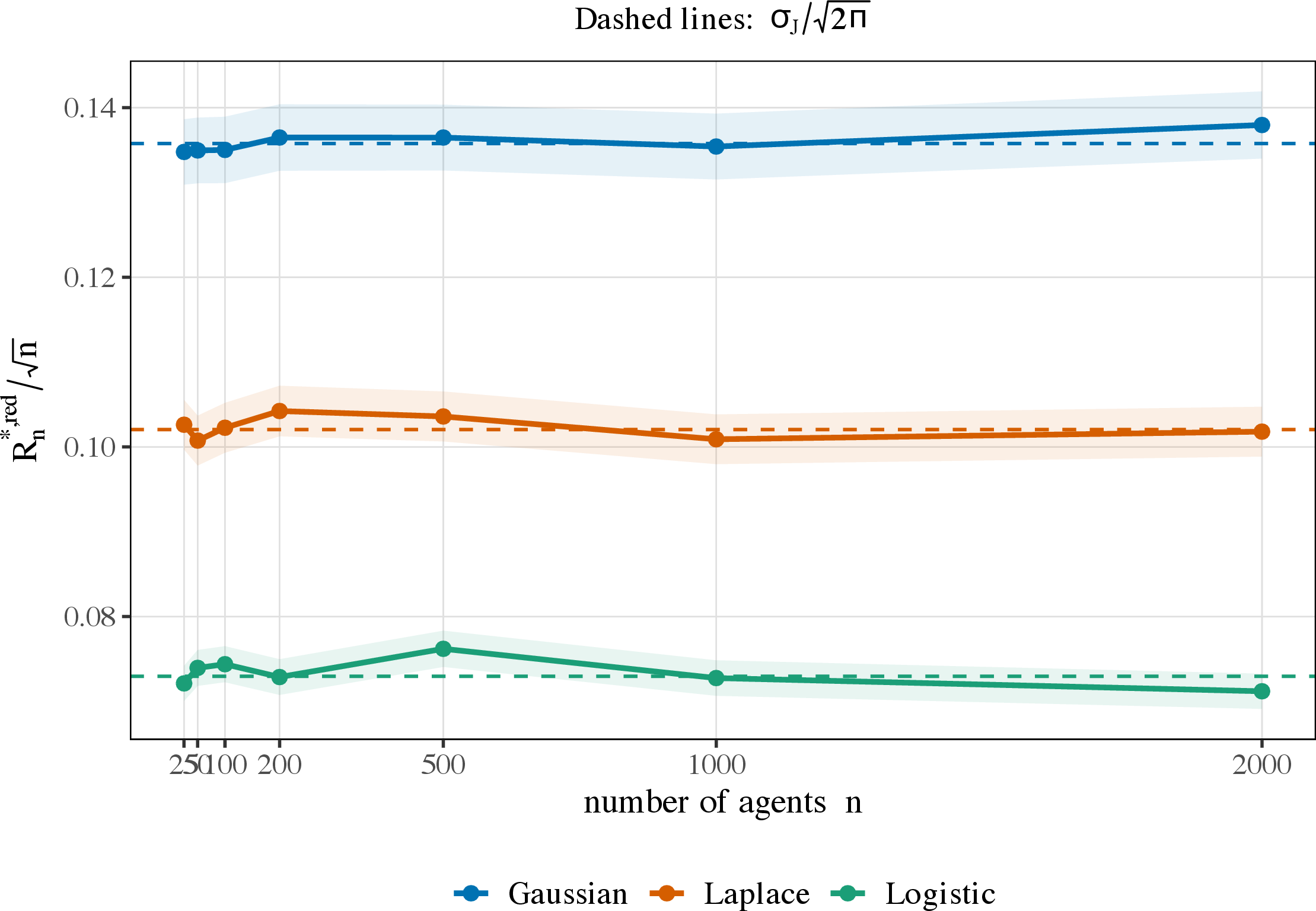
If \(\underline{x}=0\), then \[R_n^{*,\mathrm{red}}(K) = \frac{\sigma_J}{\sqrt{2\pi}}\sqrt n + o(\sqrt n).\]
If \(\underline{x}<0\), define the Cramér rate function \[\label{eq:known95prior95rate95function} I_K(a) = \sup_{t\in\mathbb{R}} \left\{ ta-\log\mathbb{E}[e^{t\widehat J_i(Y_i)}] \right\}.\tag{58}\] If \(0\) lies in the interior of the convex hull of \(\mathop{\mathrm{supp}}\widehat J_i(Y_i)\), then \[\lim_{n\to\infty} \frac{1}{n} \log R_n^{*,\mathrm{red}}(K) = -I_K(0) < 0.\]
Proof. Appendix 9.6.
The theorem concerns maximum reduced-form revenue. Equality with revenue in the original mechanism problem requires that the envelope payment generated by \(q^{\mathrm{rev}}\) satisfy the range condition in Proposition 1.
Remark 7 (Probability and revenue in the negative-drift regime). When \(\underline{x}<0\), Cramér’s theorem also gives \[\lim_{n\to\infty} \frac{1}{n} \log\mathbb{P}(V_n\ge0) = -I_K(0).\] Thus the probability of positive aggregate posterior virtual surplus and maximum reduced-form revenue have the same exponential decay exponent \(I_K(0)\), although they are distinct finite-sample quantities.
4.4 Revenue of a Fixed Posterior-Score Rule↩︎
For \(\lambda\ge0\), let \(W_i(\lambda)=\widehat x_i(Y_i)+\lambda\widehat J_i(Y_i)=S_i(Y_i,\lambda)\) and let \[\label{eq:mean95score95def} \mu_S(\lambda) = \mathbb{E}[S_i(Y_i,\lambda)] = \mathbb{E}[X]+\lambda\,\underline{x}\tag{59}\] denote the per-agent mean posterior score; consider \(q_\lambda(Y)=\mathbf{1}\{\sum_iW_i(\lambda)\ge0\}\).
Proposition 2 (Revenue of a fixed posterior-score rule). Fix \(\lambda\ge0\) with \(\mu_S(\lambda)>0\). Then there exist constants \(c_\lambda,C_\lambda>0\) such that \[\label{eq:fixed95rule95acceptance} \mathbb{P}(q_\lambda(Y)=0) \le C_\lambda e^{-c_\lambda n},\qquad{(4)}\] and \[\label{eq:fixed95rule95revenue95asymptotics} \mathbb{E}[V_n(Y)q_\lambda(Y)] = n\underline{x} + \mathcal{O}\!\left(ne^{-c_\lambda n}\right).\qquad{(5)}\] Consequently, the rule generates positive linear-order revenue when \(\underline{x}>0\) and a negative linear-order deficit when \(\underline{x}<0\).
Proof. Appendix 9.7.
Remark 8 (Knife-edge multiplier). Suppose \(\underline{x}\ne0\). The mean score vanishes at \(\lambda_{\mathrm{crit}}=-\mathbb{E}[X]/\underline{x}\), provided this is nonnegative. If \(\underline{x}<0\), then \(\mu_S(\lambda)\) is decreasing, so implementation converges to one for fixed \(\lambda<\lambda_{\mathrm{crit}}\) and to zero for fixed \(\lambda>\lambda_{\mathrm{crit}}\); if \(\underline{x}>0\) the direction is reversed. A nondegenerate local transition requires a sequence \(\lambda_n-\lambda_{\mathrm{crit}}=\mathcal{O}(n^{-1/2})\) and follows from a separate central-limit calculation rather than directly from Proposition 2.
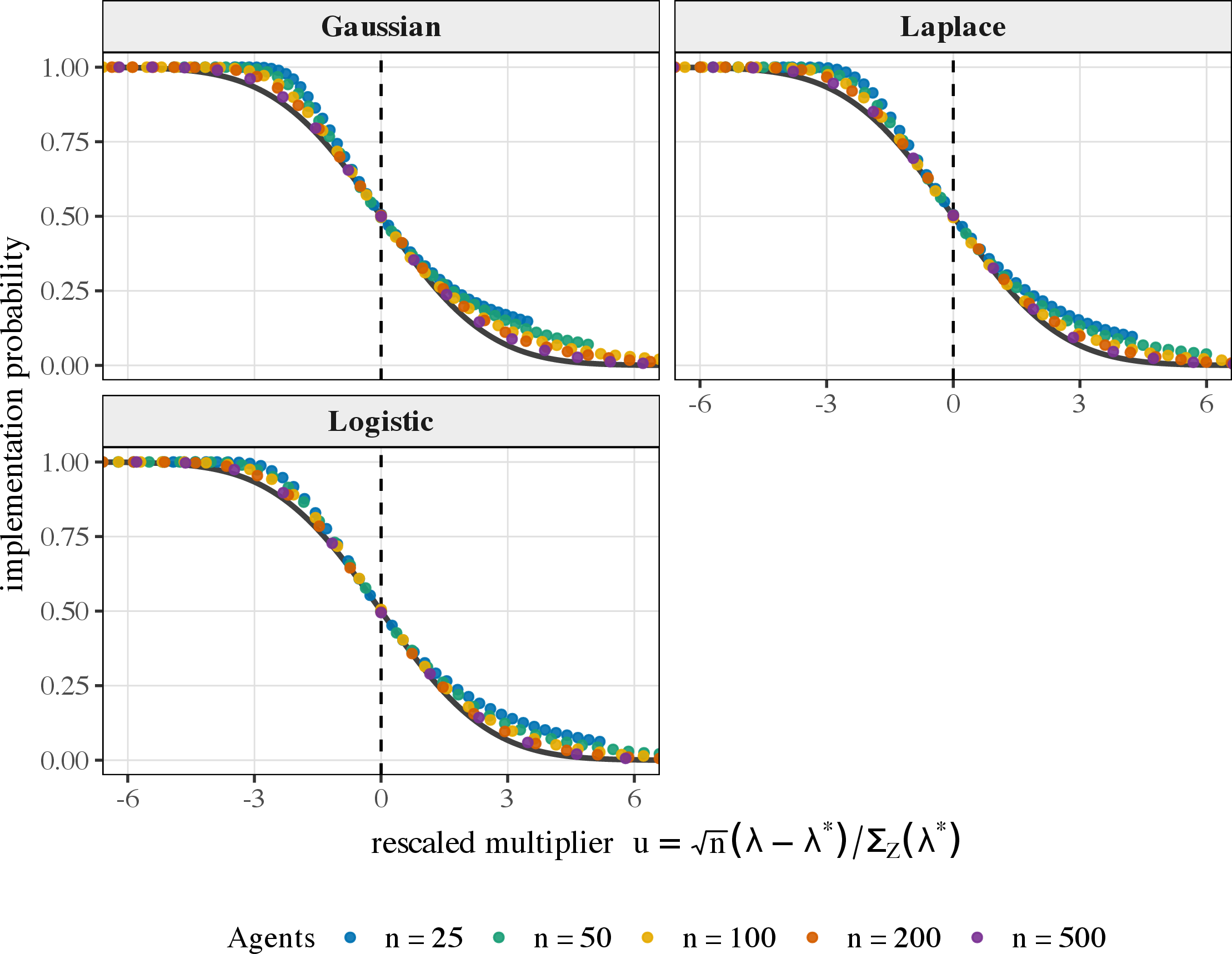
Proposition 3 (Local transition at the mean-score boundary). Suppose \(\underline{x}\ne0\), let \[\lambda_{\mathrm{crit}} = -\frac{\mathbb{E}[X]}{\underline{x}} \ge0,\] and assume \[\sigma_{\mathrm{crit}}^2 = \mathop{\mathrm{Var}}\!\left( S_i(Y_i,\lambda_{\mathrm{crit}}) \right) \in(0,\infty).\] For a fixed \(h\in\mathbb{R}\), let \[\lambda_n = \lambda_{\mathrm{crit}} + \frac{h}{\sqrt n}.\] Then \[\label{eq:local95multiplier95transition} \mathbb{P}\!\left( \sum_{i=1}^{n} S_i(Y_i,\lambda_n) \ge0 \right) \longrightarrow \Phi\!\left( \frac{h\underline{x}}{\sigma_{\mathrm{crit}}} \right).\qquad{(6)}\] Equivalently, defining \[u_n = -\frac{ \sqrt n\,\underline{x} (\lambda_n-\lambda_{\mathrm{crit}}) }{ \sigma_{\mathrm{crit}} },\] the implementation probability converges to \(\Phi(-u)\) whenever \(u_n\to u\).
Proof. Appendix 9.8.
4.5 Hierarchical Prior↩︎
Let \(\theta\sim\pi\). Conditional on \(\theta\), suppose \(X_1,\ldots,X_n\overset{\mathrm{iid}}{\sim}F_\theta\) on the common support \(\mathcal{X}=[\underline{x},\bar{x}]\). Agents observe \(\theta\), while the planner observes only \(Y\); incentive compatibility and individual rationality are imposed conditional on \(\theta\). For every \(\theta\), define \(\widehat x^\theta(y_i)=\mathbb{E}[X_i\mid\theta,Y_i=y_i]\), \(\widehat J^\theta(y_i)=\mathbb{E}[J_\theta(X_i)\mid\theta,Y_i=y_i]\), and the hierarchical per-agent and aggregate scores \[\label{eq:hierarchical95score} \Psi_i(y,\lambda) = \mathbb{E}_{\theta\mid y} \left[ \widehat x^\theta(y_i) + \lambda\widehat J^\theta(y_i) \right], \qquad G_\lambda^{\mathrm H}(y) = \sum_{i=1}^{n}\Psi_i(y,\lambda).\tag{60}\] Unlike the known-prior score, \(\Psi_i(y,\lambda)\) generally depends on the entire signal profile through the posterior of \(\theta\). We first study a conditional reduced-form relaxation. In this relaxation, for each value of \(\theta\), the allocation must induce a conditionally monotone interim allocation and therefore admits a \(\theta\)-indexed envelope-payment schedule. Because the planner does not observe \(\theta\), these conditional payment schedules need not be jointly implementable by a single signal-measurable ex-post transfer. Full implementation therefore requires the additional simultaneous Fredholm compatibility condition described in Remark 10.
Theorem 3 (Hierarchical posterior-score allocation). Suppose Assumptions 6, 7, and 8 of Appendix 9.9 hold. Suppose further that the hierarchical reduced-form revenue requirement is strictly feasible: there exists an allocation \(q_{\mathrm H}^{\circ}\) that induces a weakly increasing conditional interim allocation for every \(\theta\) and satisfies \[\mathsf V_{\mathrm H}(q_{\mathrm H}^{\circ}) > R.\] Then there exists a finite multiplier \(\lambda^{*}\ge0\) such that \[\label{eq:hierarchical95optimal95allocation} q_{\mathrm H}^*(y) = \mathbf{1}\!\left\{ G_{\lambda^{*}}^{\mathrm H}(y)>0 \right\} \qquad \text{almost surely under the hierarchical truthful signal law}\tag{61}\] solves the hierarchical conditional reduced-form allocation problem. For every \(\theta\), it induces a weakly increasing conditional interim allocation and therefore admits a \(\theta\)-indexed conditional envelope payment schedule. Moreover, \[\lambda^{*} \left( \mathsf V_{\mathrm H}(q_{\mathrm H}^*)-R \right) = 0.\]
Proof. Appendix 9.9.
Remark 9 (Scope of the hierarchical theorem). Theorem 3 solves a conditional reduced-form relaxation. It does not by itself establish the existence of a single signal-measurable transfer \(t_i(Y)\) that implements all of the \(\theta\)-indexed conditional envelope-payment schedules simultaneously. Accordingly, the value of the relaxation is an upper bound on the value of the fully implementable hierarchical mechanism problem unless the simultaneous range condition in Remark 10 is verified.
The theorem also assumes a common conditional support \([\underline{x},\bar{x}]\) for all \(\theta\). A model in which \(\theta\) is itself an unknown endpoint, such as \(X_i\mid\theta\sim\mathop{\mathrm{Unif}}[\underline{x},\theta]\), has \(\theta\)-dependent support and is nonregular; it may be studied numerically but is not covered by Theorem 3.
Remark 10 (Hierarchical transfer implementation). Full implementation requires a single signal-measurable transfer \(t_i:\mathcal{Y}^n\to\mathbb{R}\) to satisfy the conditional Fredholm equation for every \(\theta\). Conditional completeness identifies the corresponding conditional opponent average whenever a solution exists, but it does not imply that the family of required conditional interim payments lies in the joint range generated by one common ex-post transfer. Thus conditional envelope implementability for each \(\theta\) separately is necessary but not sufficient for implementation in the original hierarchical mechanism.
4.6 Welfare Comparisons across Channels↩︎
Let \(\mathcal{Q}^{\mathrm{mon}}(K)\) denote the reduced-form allocation rules that induce weakly increasing interim allocations under channel \(K\), and define \[\label{eq:reduced95value95channel} W^{\mathrm{red}}(R;K) = \sup_{q\in\mathcal{Q}^{\mathrm{mon}}(K)} \left\{ \mathbb{E}\!\left[ q(Y)\sum_{i=1}^{n}\widehat x_i(Y_i) \right]: \mathbb{E}\!\left[ q(Y)\sum_{i=1}^{n}\widehat J_i(Y_i) \right] \ge R \right\}.\tag{62}\]
Proposition 4 (Blackwell monotonicity). If \(K_1\succeq_{\mathrm B}K_2\), then \[\label{eq:blackwell95value95monotonicity} W^{\mathrm{red}}(R;K_1) \ge W^{\mathrm{red}}(R;K_2)\qquad{(7)}\] for every prior, population size, and revenue target that is reduced-form feasible under \(K_2\).
Proof. Appendix 9.10.
Remark 11 (Reduced-form versus full implementation). Proposition 4 compares reduced-form values. Equality with the value of the original mechanism problem additionally requires transfer implementation under the relevant channel.
4.6.1 Equal-Scale Laplace–Logistic Comparison↩︎
Proposition 5 (Laplace dominates logistic at equal scale). For every \(s>0\), \[\label{eq:equal95scale95blackwell95order} K_{\mathrm{Lap},s} \succeq_{\mathrm B} K_{\mathrm{Log},s},\qquad{(8)}\] and hence \(W^{\mathrm{red}}(R;K_{\mathrm{Lap},s})\ge W^{\mathrm{red}}(R;K_{\mathrm{Log},s})\). Since both channels have pure-LDP frontier scale \(s=\Delta_{\mathcal{X}}/\epsilon\), the same ordering holds under a common pure-\(\epsilon\) calibration.
Proof. Appendix 7.7.
4.6.2 Common Tight-\(\mu\) Calibration↩︎
Let \(\mu_K(s)\) denote the smallest GDP parameter for which the channel at scale \(s\) satisfies \(\mu_K(s)\)-GDP.
Proposition 6 (Common tight-\(\mu\) frontier scales). For every \(\mu>0\), the Gaussian, Laplace, and logistic frontier scales are \[\label{eq:common95mu95scales} \sigma^*(\mu) = \frac{\Delta_{\mathcal{X}}}{\mu}, \qquad b_L^*(\mu) = \frac{\Delta_{\mathcal{X}}}{-2\log\!\bigl(2\Phi(-\mu/2)\bigr)}, \qquad \beta^*(\mu) = \frac{\Delta_{\mathcal{X}}}{2\log\!\bigl( \Phi(\mu/2)/\Phi(-\mu/2) \bigr)}.\qquad{(9)}\] They satisfy \(\mu_G(\sigma^*(\mu))=\mu_L(b_L^*(\mu))=\mu_{\mathrm{Log}}(\beta^*(\mu))=\mu\) and \[\label{eq:main95scale95ordering} \beta^*(\mu) < b_L^*(\mu).\qquad{(10)}\] For each family, the least-private pair over \(\mathcal{X}\) is \((\underline{x},\bar{x})\).
Proof. Appendix 7.4.
Because \(\beta^*(\mu)<b_L^*(\mu)\), the common-\(\mu\) comparison is not an equal-scale comparison, so Proposition 5 does not determine the ordering under this calibration.
4.6.3 Endpoint Dominance under Common Tight \(\mu\)↩︎
Restrict the report space to the binary endpoint state space \(\{\underline{x},\bar{x}\}\), and let \(K_{\mathrm{Lap},\mu}^{\mathrm{end}}\) and \(K_{\mathrm{Log},\mu}^{\mathrm{end}}\) denote the tightly calibrated endpoint experiments.
Theorem 4 (Endpoint dominance at common \(\mu\)-GDP). For every \(\mu>0\), \[\label{eq:endpoint95tradeoff95order} \mathcal{T}_{\mathrm{Log},\mu}^{\mathrm{end}}(\alpha) \le \mathcal{T}_{\mathrm{Lap},\mu}^{\mathrm{end}}(\alpha) \qquad \forall\alpha\in[0,1],\tag{63}\] equivalently \(K_{\mathrm{Log},\mu}^{\mathrm{end}}\succeq_{\mathrm B} K_{\mathrm{Lap},\mu}^{\mathrm{end}}\). Therefore, for every endpoint-state decision problem, \[\label{eq:endpoint95welfare95order} W_{\mathrm{end}}^{\mathrm{red}} \!\left( R;K_{\mathrm{Log},\mu}^{\mathrm{end}} \right) \ge W_{\mathrm{end}}^{\mathrm{red}} \!\left( R;K_{\mathrm{Lap},\mu}^{\mathrm{end}} \right)\tag{64}\] whenever the revenue target is feasible under the Laplace endpoint experiment.
Proof. Appendix 7.8.
Remark 12 (Scope of the endpoint theorem). Theorem 4 applies only to the binary subexperiment generated by the maximally separated reports \(\underline{x}\) and \(\bar{x}\). It does not establish a Blackwell ordering between the tightly calibrated Laplace and logistic channels on the full continuous report space.
Remark 13 (Gaussian benchmark). At \(\sigma^*(\mu)=\Delta_{\mathcal{X}}/\mu\), the Gaussian endpoint experiment has trade-off function \(G_\mu\) at every testing level. The tightly calibrated Laplace and logistic endpoint trade-off functions satisfy \(\mathcal{T}(\alpha)\ge G_\mu(\alpha)\), with equality at \(\alpha\in\{0,\Phi(-\mu/2),1\}\) and strict inequality at every other interior testing level.
Outside the exact comparisons above, no universal ranking of the Gaussian, Laplace, and logistic channels is asserted. The numerical comparisons in Section 5.4 are therefore specification dependent unless supported by Proposition 5 or Theorem 4.
5 Numerical Illustrations↩︎
This section 4 connects the main results to simulation. The four experiments trace, in turn, the price the planner pays for privacy in the responsiveness of provision, the knife-edge at which budget pressure switches a public good from always funded to never funded, the difficulty of financing provision when the marginal agent is break-even, and the channel-choice problem a regulator faces once privacy is budgeted in an economically meaningful unit. Throughout we use the three additive channels of Table 1—Gaussian \(Y=X+\eta^{G}\), Laplace \(Y=X+\eta^{L}\), and logistic \(Y=X+\eta^{\mathrm{Log}}\)—and a uniform type distribution, with the support chosen in each experiment to probe the relevant regime. Posterior moments \(\widehat x(y)=\mathbb{E}[X\mid Y=y]\) and \(\widehat J(y)=\mathbb{E}[J(X)\mid Y=y]\) are evaluated by quadrature against the prior; implementation frequencies and revenue are estimated by Monte Carlo with common random numbers across channels, so that channel comparisons are paired. The priors and privacy calibrations used in each experiment are recorded in Appendix 10.
5.1 The Price of Privacy in the Provision Rule↩︎
The optimal rule of Theorem 1 provides the public good when the aggregate posterior score \(G_\lambda=\sum_i S_i\) is positive (under the no-mass condition the threshold set is null, so the value assigned on \(\{G_\lambda=0\}\) is immaterial). Economically, each per-agent score \[S_i(y_i,\lambda) = \underbrace{\widehat x_i(y_i)}_{\text{expected value}} + \lambda\, \underbrace{\widehat J_i(y_i)}_{\text{revenue net of rents}}, \qquad J(x)=x-\frac{1-F(x)}{f(x)},\] is the planner’s case for building attributable to agent \(i\): the agent’s expected value for the good plus the revenue that can be extracted from that agent net of the information rent the agent commands, the two priced against each other by the shadow value \(\lambda\ge0\) of the revenue requirement. The privacy channel enters only through how sharply this case responds to the agent’s noisy report.
Figure 2 plots \(S(\cdot,\lambda)\) for each channel on a uniform prior. The Gaussian and logistic scores rise strictly with the signal: every report, however extreme, still moves the provision decision, so the good remains responsive to the private intensity of an agent’s preference. Under Laplace noise, the score varies over the interior region \(y\in(\underline{x},\bar{x})\) and is exactly flat on the global tails \(y\le\underline{x}\) and \(y\ge\bar{x}\): the privacy mechanism has pooled all sufficiently enthusiastic (or sufficiently reluctant) reporters into a single indistinguishable group, because the bounded prior makes the Laplace likelihood ratio constant in the tails (Remark 2). For those agents, expressing more enthusiasm buys no additional weight in the decision. The economic content of the channel is thus an elasticity: privacy noise governs how strongly public provision can track private values, and a coarser channel caps that responsiveness precisely for the types whose preferences are most extreme.
![Figure 2: The per-agent score S(y,\lambda)=\widehat x(y)+\lambda\widehat J(y)—the planner’s case for building attributable to one agent—against that agent’s report y, for the three channels and several values of the revenue price \lambda. Gaussian and logistic respond to every report (strict MLRP), so provision stays sensitive to private value; Laplace is flat outside [\underline{x},\bar{x}] (tail pooling), so privacy caps how far provision can respond for the most extreme types. This score is the object thresholded by the optimal rule of Theorem 1.](/article/2606.24013/figures/fig_exp1_posterior_score_panel.png "fig:")
5.2 When Budget Pressure Switches the Good Off↩︎
The multiplier \(\lambda\) is the weight the planner places on revenue relative to welfare, and Proposition 2 shows that whether the good is funded is governed by the per-agent mean score \[\mu_S(\lambda)=\mathbb{E}[X]+\lambda\,\underline{x},\] the average net social value the planner perceives once revenue is priced at \(\lambda\). The decisive primitive is \(\underline{x}=\mathbb{E}[\widehat J_i(Y_i)]\) (Lemma 11), the lower endpoint of the type distribution, equal to the mean posterior virtual value, i.e.the average virtual surplus per agent. The mean score changes sign at the critical price \[\lambda_{\mathrm{crit}} = -\,\mathbb{E}[X]/\underline{x},\] where \(\mu_S(\lambda_{\mathrm{crit}})=0\). In the numerical design \(X\sim\mathop{\mathrm{Unif}}[-0.5,1.5]\), so \(\underline{x}<0\) and \(\mu_S'(\lambda)=\underline{x}<0\); hence \(\mu_S(\lambda)>0\) for \(\lambda<\lambda_{\mathrm{crit}}\) and \(\mu_S(\lambda)<0\) for \(\lambda>\lambda_{\mathrm{crit}}\), and by the law of large numbers the good is funded with probability tending to one for \(\lambda<\lambda_{\mathrm{crit}}\) and to zero for \(\lambda>\lambda_{\mathrm{crit}}\) (the two directions exchange when \(\underline{x}>0\)). The economic reading is stark: as the population grows the public good is essentially always provided while the budget is loose and essentially never provided once it tightens past \(\lambda_{\mathrm{crit}}\), with no smooth interior trade-off. A small increase in fiscal pressure can flip a project from “always built” to “never built.”
How privacy bears on this cliff is the content of the central-limit refinement. A separate local calculation around \(\lambda_{\mathrm{crit}}\), applied to sequences satisfying \(\sqrt n\,(\lambda_n-\lambda_{\mathrm{crit}})=O(1)\), gives a funding probability of approximately \(\Phi\!\big(\sqrt n\,\mu_S(\lambda)/\sigma_S(\lambda_{\mathrm{crit}})\big)\), where \(\sigma_S^2(\lambda_{\mathrm{crit}})=\mathop{\mathrm{Var}}\!\big(S_i(Y_i,\lambda_{\mathrm{crit}})\big)\). Writing the standardized budget pressure \[u = -\,\frac{\sqrt n\,\mu_S(\lambda)}{\sigma_S(\lambda_{\mathrm{crit}})} = -\,\frac{\sqrt n\,\underline{x}\,(\lambda-\lambda_{\mathrm{crit}})}{\sigma_S(\lambda_{\mathrm{crit}})},\] which absorbs the constant slope \(\mu_S'(\lambda_{\mathrm{crit}})=\underline{x}\), the probability converges to \(\Phi(-u)\) for every channel. Figure 3 confirms this: the curves for \(n\in\{25,\dots,500\}\) collapse onto the common Gaussian limit. For nondegenerate channels satisfying \(\sigma_S^2(\lambda_{\mathrm{crit}})>0\), the privacy channel enters the local transition through the scale \(\sigma_S(\lambda_{\mathrm{crit}})\). It stretches or compresses the transition, sharpening or blurring how precisely the planner can locate the funding margin, but it does not move the mean-score boundary \(\lambda_{\mathrm{crit}}\). The boundary is channel invariant because posterior expectations preserve the unconditional means \(\mathbb{E}[X]\) and \(\mathbb{E}[\widehat J(Y)]=\underline{x}\). Whether a public good is fundable is set by the mean posterior virtual value \(\underline{x}\), not by the privacy technology.
5.3 Financing a Good at the Break-Even Margin↩︎
Theorem 2 classifies optimal reduced-form revenue \(R_n^{*,\mathrm{red}}\) by the sign of the mean posterior virtual value \(\underline{x}\) of the previous subsection: revenue grows linearly with the market when \(\underline{x}>0\), decays when \(\underline{x}<0\), and—in the boundary case \(\underline{x}=0\)—grows only at square-root order \[R_n^{*,\mathrm{red}} \sim \frac{\sigma_J}{\sqrt{2\pi}}\,\sqrt n, \qquad \sigma_J^2=\mathop{\mathrm{Var}}\!\big(\widehat J_i(Y_i)\big).\] This boundary is the economically critical case: the lower endpoint equals zero, so average posterior virtual value has zero drift and the mechanism collects no systematic revenue. Per-capita revenue \(R_n^{*,\mathrm{red}}/n\to0\), so a privacy-respecting public-good mechanism cannot raise funds that scale with the market; what it collects comes entirely from the statistical luck of drawing a realized virtual surplus above its mean. The magnitude of that luck—and hence the financing the planner can hope for—is set by \(\sigma_J\), the informativeness of the privacy channel about types: a sharper channel raises the constant \(\sigma_J/\sqrt{2\pi}\), but no channel changes the \(\sqrt n\) rate. Figure 4 verifies both the rate and the constant, with the normalized revenue \(R_n^{*,\mathrm{red}}/\sqrt n\) flattening onto each channel’s level \(\sigma_J/\sqrt{2\pi}\). The message is that financing a public good from a population whose marginal member breaks even is fundamentally hard: privacy technology can buy a better constant, but not a better order of magnitude. We display \(\underline{x}=0\) because it gives the sharpest quantitative check; the funded (\(\underline{x}>0\)) regime is governed by its leading term \(n\underline{x}\), and the starved (\(\underline{x}<0\)) regime follows from the same theorem and is illustrated in Appendix 10.
5.4 Choosing a Privacy Technology: the Welfare Reversal↩︎
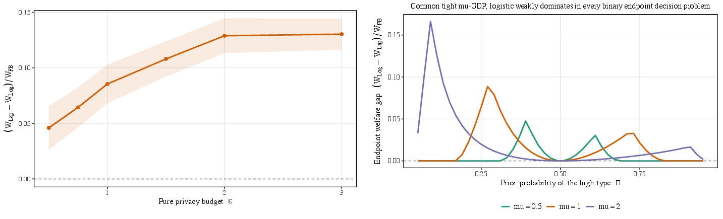
Which privacy technology should a planner adopt to maximize welfare? Figure 5 shows the answer is not a property of the noise distribution alone—it depends on the privacy-accounting standard used to hold privacy fixed. Raw noise scale, pure \(\epsilon\)-LDP, and \(\mu\)-GDP are distinct standards. For the Laplace–logistic comparison, a common noise scale is equivalent to a common tight pure-\(\epsilon\)-LDP calibration. Under this calibration, the Laplace channel Blackwell-dominates the logistic channel (Proposition 5), so \[W^{\mathrm{red}}(R;K_{\mathrm{Lap},s}) \ge W^{\mathrm{red}}(R;K_{\mathrm{Log},s}).\] Recalibrating both channels under a common tight \(\mu\)-GDP guarantee changes their relative scales and reverses the information ordering on the maximally separated endpoint experiment \(\{\underline{x},\bar{x}\}\): there the logistic channel takes the smaller scale and is the more informative experiment, so the welfare ranking flips (Theorem 4).
The left panel of Figure 5 plots the equal-scale welfare gap \((W_{\mathrm{Lap}}-W_{\mathrm{Log}})/W_{\mathrm{FB}}\ge0\) against the pure-\(\epsilon\) budget; the right panel plots the common-\(\mu\) endpoint welfare gap \((W_{\mathrm{Log}}-W_{\mathrm{Lap}})/W_{\mathrm{FB}}\ge0\) against the high-type probability, for three privacy levels \(\mu\). In each calibration the dominant channel’s welfare advantage is nonnegative, and the dominant channel flips from Laplace to logistic as the accounting standard changes from scale to GDP. The comparative reading is that no privacy channel is universally welfare-best; the welfare ranking depends on the privacy-accounting standard under which the channels are compared. We stress the scope. The reversal is established for the maximally separated endpoint experiment \(\{\underline{x},\bar{x}\}\) and does not lift to a Blackwell ranking over the full continuum of types (Remark 12); a planner therefore cannot conclude that logistic dominates Laplace under GDP for an arbitrary preference distribution. The sharp ROC-level form of the endpoint comparison, and the near-zero continuous-type gap that delimits its scope, are reported in Appendix 10.
6 Conclusion↩︎
We have studied binary public-good provision when a planner observes agents only through a fixed local-privacy channel. The privacy channel reshapes the information on which optimal provision is based: the optimal reduced-form rule thresholds an aggregate posterior score combining, for each agent, the posterior expected valuation and posterior virtual value. The channel enters through the responsiveness of this score to the agent’s privatized report.
Three economic conclusions emerge. First, the allocation the planner would like to choose and the payments needed to implement it are distinct objects. Implementing the envelope payments through transfers measurable in the privatized signals is an inverse problem governed by a Fredholm range condition: completeness gives uniqueness when a solution exists but does not guarantee existence. The Online Supplement complements this exact characterization with approximate implementations carrying explicit incentive, participation, and revenue bounds.
Second, maximum reduced-form revenue follows three asymptotic regimes governed by the lower endpoint of the valuation distribution. It is asymptotically linear, of square-root order, or exponentially small according as that endpoint is positive, zero, or negative. The privacy channel affects the quantitative difficulty within these regimes through the square-root constant and the large-deviation rate. For a fixed posterior-score rule, provision also changes sharply from asymptotically certain to asymptotically negligible at a mean-score boundary.
Third, welfare comparisons between privacy channels depend on how privacy is calibrated. For Laplace and logistic noise, a common scale is equivalent to the common tight pure-\(\epsilon\) calibration considered here, and Laplace Blackwell-dominates logistic noise on the full report space. Under a common tight \(\mu\)-GDP calibration, the ordering reverses for the maximally separated binary endpoint experiment. Thus the preferred channel may depend on the privacy standard used for comparison, while the endpoint reversal does not imply a general ordering over the full continuous type space.
The limits of these results also point to several directions for future work. The allocation and revenue results are reduced-form statements; connecting them to fully implemented mechanisms requires verifying the relevant transfer range condition. Characterizing which economically important envelope-payment schedules belong to the range of smoothing channel operators remains open. The hierarchical extension relies on a high-level coordinatewise-monotonicity condition that need not follow automatically once a latent common component links agents’ values. Identifying primitive conditions for this monotonicity, and studying the scope for surplus extraction under privatized correlated information, are natural next steps.
The channel comparisons leave a further boundary. Equal-scale Laplace-over-logistic dominance holds on the full report space, but the common-\(\mu\) reversal is established only for the endpoint experiment. Whether comparable welfare orderings hold on continuous type spaces, and how the conclusions change for nonadditive or nonsmoothing channels, remain open. More broadly, the framework suggests treating the privacy standard itself as part of the design problem: when welfare comparisons depend on the calibration used to hold privacy fixed, privacy accounting is not merely a technical convention.
7 Privacy and Channel Derivations↩︎
This appendix develops the privacy, likelihood-ratio, posterior, and comparison-of-experiments calculations used in the main text. We first derive the complete Neyman–Pearson trade-off functions for the Gaussian, Laplace, and logistic location channels. We then obtain their pure-LDP and tight GDP calibrations, establish the ordering of the common-\(\mu\) scales, describe posterior pooling under Laplace noise, derive the Gaussian posterior formula used in Example 2, and prove the two Blackwell comparisons stated in Section 4.6.
Throughout, \[\Delta_{\mathcal{X}} = \bar{x}-\underline{x}.\] For two reports \(r<r'\), write \[d=r'-r\in[0,\Delta_{\mathcal{X}}].\] For an additive location family, translation invariance reduces the binary experiment generated by \((r,r')\) to the experiment generated by locations \((0,d)\).
For probability measures \(P\) and \(Q\) on a common measurable space, recall the testing trade-off function \[\label{eq:app95tradeoff95definition} \mathcal{T}(P,Q)(\alpha) = \inf_{\psi} \left\{ 1-\mathbb{E}_Q[\psi]: \mathbb{E}_P[\psi]\le\alpha \right\}, \qquad \alpha\in[0,1],\tag{65}\] where the infimum is taken over measurable randomized tests \(\psi:\mathcal{Y}\to[0,1]\). The Neyman–Pearson lemma implies that, for each pair of simple hypotheses, the lower envelope is generated by likelihood-ratio tests.
7.1 Gaussian Location Channel↩︎
Let \[P_{0,\sigma} = \mathcal{N}(0,\sigma^2), \qquad P_{d,\sigma} = \mathcal{N}(d,\sigma^2).\] The log-likelihood ratio is \[\label{eq:app95gaussian95log95lr} \log \frac{dP_{d,\sigma}}{dP_{0,\sigma}}(y) = \frac{d}{\sigma^2}y - \frac{d^2}{2\sigma^2},\tag{66}\] which is strictly increasing in \(y\). Hence the most powerful test of \(P_{0,\sigma}\) against \(P_{d,\sigma}\) rejects for sufficiently large values of \(Y\).
For a level-\(\alpha\) test, choose \(c_\alpha\) such that \[\alpha = P_{0,\sigma}(Y\ge c_\alpha) = 1-\Phi(c_\alpha/\sigma).\] Thus \[c_\alpha = \sigma\Phi^{-1}(1-\alpha).\] The corresponding type-II error is \[P_{d,\sigma}(Y<c_\alpha) = \Phi\!\left( \frac{c_\alpha-d}{\sigma} \right).\] Therefore, \[\label{eq:app95gaussian95tradeoff} \mathcal{T}_{G,d,\sigma}(\alpha) = \Phi\!\left( \Phi^{-1}(1-\alpha)-\frac{d}{\sigma} \right) = G_{d/\sigma}(\alpha).\tag{67}\]
Proposition 7 (Gaussian privacy frontier). For the Gaussian additive channel with scale \(\sigma\), \[\label{eq:app95gaussian95tight95mu} \mu_G(\sigma) = \frac{\Delta_{\mathcal{X}}}{\sigma}.\qquad{(11)}\] The channel satisfies strict MLRP but does not satisfy finite pure \(\epsilon\)-LDP.
Proof. Equation 67 shows that the binary experiment generated by reports separated by \(d\) has GDP parameter \(d/\sigma\). The least-private report pair has the maximal separation \(d=\Delta_{\mathcal{X}}\), proving ?? .
For \(x_2>x_1\), \[\label{eq:app95gaussian95mlr} \frac{k_G(y\mid x_2)}{k_G(y\mid x_1)} = \exp\!\left\{ \frac{x_2-x_1}{\sigma^2}y - \frac{x_2^2-x_1^2}{2\sigma^2} \right\},\tag{68}\] which is strictly increasing in \(y\). Hence strict MLRP holds.
The likelihood ratio in 68 is unbounded as \(y\to\infty\), so no finite constant \(\epsilon\) can satisfy the pointwise likelihood-ratio bound required by pure LDP. ◻
7.2 Laplace Location Channel↩︎
Let \[P_{0,b} = \mathop{\mathrm{Lap}}(0,b), \qquad P_{d,b} = \mathop{\mathrm{Lap}}(d,b), \qquad \rho = \frac{d}{b}.\] The likelihood ratio is \[\label{eq:app95laplace95lr} \frac{k_L(y\mid d)}{k_L(y\mid0)} = \exp\!\left\{ \frac{|y|-|y-d|}{b} \right\}.\tag{69}\] Equivalently, \[\label{eq:app95laplace95lr95piecewise} \frac{k_L(y\mid d)}{k_L(y\mid0)} = \begin{cases} e^{-\rho}, & y\le0, \\[3pt] e^{(2y-d)/b}, & 0<y<d, \\[3pt] e^\rho, & y\ge d. \end{cases}\tag{70}\] The ratio is weakly increasing but constant in each outer tail. Thus the Laplace channel satisfies weak, but not strict, MLRP.
Proposition 8 (Laplace trade-off function). For \(\rho=d/b\), \[\label{eq:app95laplace95tradeoff} \mathcal{T}_{L,\rho}(\alpha) = \begin{cases} 1-e^\rho\alpha, & 0\le\alpha\le \frac{1}{2}e^{-\rho}, \\[8pt] \dfrac{e^{-\rho}}{4\alpha}, & \frac{1}{2}e^{-\rho}\le\alpha\le\frac{1}{2}, \\[10pt] e^{-\rho}(1-\alpha), & \frac{1}{2}\le\alpha\le1. \end{cases}\qquad{(12)}\] Its unique interior fixed point is \[\label{eq:app95laplace95fixed95point} p_L(\rho) = \frac{1}{2}e^{-\rho/2}.\qquad{(13)}\]
Proof. By 70 , the likelihood ratio is constant on \((-\infty,0]\), strictly increasing on \((0,d)\), and constant on \([d,\infty)\). The Neyman–Pearson tests therefore proceed by first using the right tail, then moving the rejection threshold through \((0,d)\), and finally randomizing in the left flat-likelihood-ratio tail.
If the rejection threshold satisfies \(c\ge d\), then \[\alpha = P_{0,b}(Y\ge c) = \frac{1}{2}e^{-c/b},\] while \[1-\mathcal{T}_{L,\rho}(\alpha) = P_{d,b}(Y\ge c) = \frac{1}{2}e^{-(c-d)/b} = e^\rho\alpha.\] This gives the first branch.
If \(0<c<d\), then \[\alpha = \frac{1}{2}e^{-c/b},\] and \[\mathcal{T}_{L,\rho}(\alpha) = P_{d,b}(Y<c) = \frac{1}{2}e^{-(d-c)/b}.\] Since \(e^{c/b}=1/(2\alpha)\), this becomes \[\mathcal{T}_{L,\rho}(\alpha) = \frac{e^{-\rho}}{4\alpha},\] which gives the middle branch.
Reflection around the midpoint \(d/2\) exchanges the two hypotheses \(P_{0,b}\) and \(P_{d,b}\). The resulting binary experiment is symmetric, so its testing trade-off function is self-inverse: \[\mathcal{T}_{L,\rho} \bigl( \mathcal{T}_{L,\rho}(\alpha) \bigr) = \alpha.\] Applying this identity to the first branch gives the final branch \[\mathcal{T}_{L,\rho}(\alpha) = e^{-\rho}(1-\alpha), \qquad \frac{1}{2}\le\alpha\le1.\] Solving \(T(\alpha)=\alpha\) on the middle branch yields \[\alpha^2=\frac{1}{4}e^{-\rho},\] and hence ?? . ◻
Corollary 1 (Laplace pure-LDP frontier). The Laplace location channel with scale \(b\) satisfies tight pure \(\epsilon\)-LDP with \[\epsilon = \frac{\Delta_{\mathcal{X}}}{b}.\] Equivalently, \[\label{eq:app95laplace95epsilon95scale} b_L^*(\epsilon) = \frac{\Delta_{\mathcal{X}}}{\epsilon}.\tag{71}\]
Proof. Equation 70 gives \[e^{-d/b} \le \frac{k_L(y\mid r')}{k_L(y\mid r)} \le e^{d/b}.\] The worst report separation is \(d=\Delta_{\mathcal{X}}\), and the upper bound is attained in the right tail. ◻
7.3 Logistic Location Channel↩︎
The centered logistic distribution with scale \(\beta>0\) has cdf \[F_\beta(y) = \frac{1}{1+e^{-y/\beta}}\] and density \[\label{eq:app95logistic95density} g_\beta(y) = \frac{e^{-y/\beta}}{\beta(1+e^{-y/\beta})^2}.\tag{72}\] Let \[P_{0,\beta} = \mathop{\mathrm{Logistic}}(0,\beta), \qquad P_{d,\beta} = \mathop{\mathrm{Logistic}}(d,\beta), \qquad \rho = \frac{d}{\beta}.\]
Proposition 9 (Logistic trade-off function). For \(\rho=d/\beta\), \[\label{eq:app95logistic95tradeoff} \mathcal{T}_{\mathrm{Log},\rho}(\alpha) = \frac{1-\alpha}{1-\alpha+e^\rho\alpha}.\qquad{(14)}\] Its unique interior fixed point is \[\label{eq:app95logistic95fixed95point} p_{\mathrm{Log}}(\rho) = \frac{1}{1+e^{\rho/2}}.\qquad{(15)}\]
Proof. The logistic location family has monotone likelihood ratio, so the Neyman–Pearson test rejects for \(Y\ge c\). Under the null, \[\alpha = 1-F_\beta(c).\] Hence \[e^{c/\beta} = \frac{1-\alpha}{\alpha}.\] Under the alternative, the type-II error is \[F_\beta(c-d) = \frac{1}{1+\exp\{-(c-d)/\beta\}}.\] Substituting the expression for \(e^{c/\beta}\) gives \[F_\beta(c-d) = \frac{1-\alpha}{1-\alpha+e^\rho\alpha}.\] Solving \(T(\alpha)=\alpha\) yields \[\frac{1-\alpha}{1-\alpha+e^\rho\alpha} = \alpha,\] whose unique interior solution is \[\alpha = \frac{1}{1+e^{\rho/2}}.\] ◻
Proposition 10 (Logistic MLRP and pure-LDP frontier). The logistic location channel satisfies strict MLRP. Its tight pure-LDP parameter over \(\mathcal{X}\) is \[\epsilon = \frac{\Delta_{\mathcal{X}}}{\beta},\] or equivalently \[\label{eq:app95logistic95epsilon95scale} \beta^*(\epsilon) = \frac{\Delta_{\mathcal{X}}}{\epsilon}.\qquad{(16)}\]
Proof. Differentiating the centered log density gives \[\frac{d}{dy}\log g_\beta(y) = -\frac{1}{\beta} + \frac{2}{\beta(1+e^{y/\beta})}.\] This derivative is strictly decreasing. Therefore, for \(x_2>x_1\), \[\frac{d}{dy} \log \frac{k_{\mathrm{Log}}(y\mid x_2)}{k_{\mathrm{Log}}(y\mid x_1)} = \frac{d}{dy}\log g_\beta(y-x_2) - \frac{d}{dy}\log g_\beta(y-x_1) > 0.\] Hence strict MLRP holds.
Moreover, \[\left| \frac{d}{dy}\log g_\beta(y) \right| \le \frac{1}{\beta}.\] By the mean-value theorem, \[\left| \log \frac{k_{\mathrm{Log}}(y\mid r)}{k_{\mathrm{Log}}(y\mid r')} \right| \le \frac{|r-r'|}{\beta}.\] The bound is approached in the tails, so it is tight. Maximizing \(|r-r'|\) over \(\mathcal{X}\) gives the result. ◻
7.4 Tight GDP Indices and Common-\(\mu\) Scales↩︎
For a trade-off function \(T\), define its Gaussian separation profile by \[\label{eq:app95gaussian95separation} D_T(\alpha) = -\Phi^{-1}(\alpha) - \Phi^{-1}(T(\alpha)), \qquad \alpha\in(0,1).\tag{73}\] Because \[G_\mu(\alpha) = \Phi\!\left( -\Phi^{-1}(\alpha)-\mu \right),\] the inequality \[T(\alpha)\ge G_\mu(\alpha)\] is equivalent to \[D_T(\alpha)\le\mu.\] Consequently, the tight GDP index of \(T\) is \[\label{eq:app95tight95mu95functional} \mu(T) = \sup_{\alpha\in(0,1)}D_T(\alpha).\tag{74}\]
Lemma 1 (Normal-quantile monotonicity). Let \[I(u) = \varphi\!\left(\Phi^{-1}(u)\right), \qquad u\in(0,1),\] and define \[A(u) = \frac{u}{I(u)}, \qquad B(u) = \frac{u(1-u)}{I(u)}.\] Then \(A\) is strictly increasing on \((0,1)\). Moreover, \(B\) is symmetric about \(1/2\) and strictly increasing on \((0,1/2)\).
These properties are closely related to classical monotonicity and functional inequalities for the Gaussian Mills ratio; see, for example, [31].
Proof. Write \[z=\Phi^{-1}(u).\] Since \[\frac{dz}{du} = \frac{1}{\varphi(z)} = \frac{1}{I(u)}\] and \[\varphi'(z)=-z\varphi(z),\] the Gaussian isoperimetric function satisfies \[\label{eq:app95gaussian95isoperimetric95derivatives} I'(u)=-z, \qquad I''(u)=-\frac{1}{I(u)}.\tag{75}\]
We first prove the monotonicity of \(A\). Differentiation gives \[A'(u) = \frac{I(u)-uI'(u)}{I(u)^2} = \frac{\varphi(z)+uz}{\varphi(z)^2}.\] If \(z\ge0\), the numerator is strictly positive. If \(z=-x<0\), then \(x>0\), \(u=\Phi(-x)\), and the numerator becomes \[\varphi(x)-x\Phi(-x).\] Moreover, \[x\Phi(-x) = x\int_x^\infty \varphi(t)\,dt < \int_x^\infty t\varphi(t)\,dt = \varphi(x),\] where the strict inequality follows from \(t>x\) on a set of positive Lebesgue measure and the final equality follows from \(\varphi'(t)=-t\varphi(t)\). Thus \(A'(u)>0\) for every \(u\in(0,1)\).
We next consider \(B\). Since \[\Phi^{-1}(1-u)=-\Phi^{-1}(u)\] and \(\varphi\) is even, \[I(1-u)=I(u).\] Consequently, \[B(1-u)=B(u),\] so \(B\) is symmetric about \(1/2\).
It remains to prove that \(B\) is strictly increasing on \((0,1/2)\). Let \[J(u)=u(1-u)\] and define \[W(u) = J'(u)I(u)-J(u)I'(u).\] Because \[B'(u) = \frac{J'(u)I(u)-J(u)I'(u)}{I(u)^2} = \frac{W(u)}{I(u)^2},\] it is enough to prove \[W(u)>0, \qquad 0<u<\frac{1}{2}.\]
Introduce the auxiliary function \[H(u) = 2I(u)^2-J(u).\] Using 75 , we obtain \[H'(u) = 4I(u)I'(u)-(1-2u)\] and \[\begin{align} H''(u) &= 4\left\{ I'(u)^2+I(u)I''(u) \right\}+2 \notag\\ &= 4\left\{ \Phi^{-1}(u)^2-1 \right\}+2 \notag\\ &= 4\Phi^{-1}(u)^2-2. \label{eq:app95H95second95derivative} \end{align}\tag{76}\] Set \[u_0 = \Phi\!\left(-\frac{1}{\sqrt2}\right).\] Equation 76 shows that \(H'\) is strictly increasing on \((0,u_0)\) and strictly decreasing on \((u_0,1/2)\).
As \(u\downarrow0\), \[I(u)\longrightarrow0\] and \[u\left|\Phi^{-1}(u)\right| \longrightarrow0.\] Indeed, writing \(u=\Phi(-x)\) with \(x\to\infty\), the inequality already proved above gives \[0\le x\Phi(-x)<\varphi(x)\longrightarrow0.\] It follows that \[\lim_{u\downarrow0}H(u)=0\] and \[\lim_{u\downarrow0}H'(u)=-1.\] At the midpoint, \[H\!\left(\frac{1}{2}\right) = 2\varphi(0)^2-\frac{1}{4} = \frac{1}{\pi}-\frac{1}{4} > 0,\] and \[H'\!\left(\frac{1}{2}\right)=0.\]
Because \(H'\) is strictly decreasing on \((u_0,1/2)\) and ends at zero, \[H'(u)>0, \qquad u_0\le u<\frac{1}{2}.\] Since \(H'\) starts at \(-1\) and is strictly increasing on \((0,u_0)\), it has exactly one zero in \((0,u_0)\). Thus \(H\) first decreases and then strictly increases on \((0,1/2)\). Since \[H(0+)=0, \qquad H\!\left(\frac{1}{2}\right)>0,\] there exists a unique \[u_*\in\left(0,\frac{1}{2}\right)\] such that \[H(u)<0 \quad\text{for }0<u<u_*, \qquad H(u)>0 \quad\text{for }u_*<u<\frac{1}{2}.\]
Differentiating \(W\) and using 75 yields \[\begin{align} W'(u) &= J''(u)I(u)-J(u)I''(u) \notag\\ &= -2I(u)+\frac{J(u)}{I(u)} \notag\\ &= -\frac{H(u)}{I(u)}. \label{eq:app95W95derivative} \end{align}\tag{77}\] Therefore, \[W'(u)>0 \quad\text{for }0<u<u_*, \qquad W'(u)<0 \quad\text{for }u_*<u<\frac{1}{2}.\]
Finally, \[\lim_{u\downarrow0}W(u)=0.\] Indeed, \(J'(u)I(u)\to0\), while \[|J(u)I'(u)| = u(1-u)\left|\Phi^{-1}(u)\right| \longrightarrow0.\] Also, \[W\!\left(\frac{1}{2}\right)=0,\] because \[J'\!\left(\frac{1}{2}\right)=0 \qquad\text{and}\qquad I'\!\left(\frac{1}{2}\right)=0.\] Thus \(W\) increases strictly from zero on \((0,u_*)\) and then decreases strictly back to zero on \((u_*,1/2)\). Hence \[W(u)>0, \qquad 0<u<\frac{1}{2}.\] Since \(I(u)>0\), it follows that \[B'(u) = \frac{W(u)}{I(u)^2} > 0, \qquad 0<u<\frac{1}{2}.\] Therefore \(B\) is strictly increasing on \((0,1/2)\). ◻
Lemma 2 (Tight endpoint GDP indices). For the Laplace and logistic endpoint experiments, \[\begin{align} \mu_L(\rho) &= -2\Phi^{-1} \left( \frac{1}{2}e^{-\rho/2} \right), \tag{78} \\ \mu_{\mathrm{Log}}(\rho) &= -2\Phi^{-1} \left( \frac{1}{1+e^{\rho/2}} \right). \tag{79} \end{align}\]
Proof. Both trade-off functions are self-inverse: \[T(T(\alpha)) = \alpha.\] Hence \[D_T(T(\alpha)) = D_T(\alpha).\] It is therefore enough to show that \(D_T\) increases up to the unique interior fixed point.
At differentiability points, \[\label{eq:app95D95derivative} D_T'(\alpha) = -\frac{1}{\varphi(\Phi^{-1}(\alpha))} - \frac{T'(\alpha)}{\varphi(\Phi^{-1}(T(\alpha)))}.\tag{80}\]
For the Laplace trade-off function, on the first branch define \[u=e^\rho\alpha=1-T_L(\alpha).\] Since \(u>\alpha\), normal symmetry and Lemma 1 give \[D_{T_L}'(\alpha) = \frac{1}{\alpha} \bigl( A(u)-A(\alpha) \bigr) > 0.\] On the middle branch, \[T_L(\alpha) = \frac{p_L(\rho)^2}{\alpha}, \qquad -T_L'(\alpha) = \frac{T_L(\alpha)}{\alpha},\] so \[D_{T_L}'(\alpha) = \frac{1}{\alpha} \bigl( A(T_L(\alpha))-A(\alpha) \bigr) > 0\] before the fixed point. Self-inversion then gives strict decrease after the fixed point. Therefore the supremum occurs at \(p_L(\rho)\), giving 78 .
For the logistic trade-off function, \[-T_{\mathrm{Log}}'(\alpha) = \frac{ T_{\mathrm{Log}}(\alpha) \{1-T_{\mathrm{Log}}(\alpha)\} }{ \alpha(1-\alpha) }.\] Substitution into 80 yields \[D_{T_{\mathrm{Log}}}'(\alpha) = \frac{ B(T_{\mathrm{Log}}(\alpha))-B(\alpha) }{ \alpha(1-\alpha) }.\] Before the fixed point, \[T_{\mathrm{Log}}(\alpha)>\alpha.\] Using the symmetry and strict increase of \(B\) on \((0,1/2)\), the numerator is positive. Hence the supremum occurs at the fixed point \(p_{\mathrm{Log}}(\rho)\), proving 79 . ◻
Solving \(\mu_L(\rho)=\mu\) gives \[\label{eq:app95laplace95rho95mu} \rho_L^*(\mu) = -2\log\!\bigl(2\Phi(-\mu/2)\bigr),\tag{81}\] while solving \(\mu_{\mathrm{Log}}(\rho)=\mu\) gives \[\label{eq:app95logistic95rho95mu} \rho_{\mathrm{Log}}^*(\mu) = 2\log\!\left( \frac{\Phi(\mu/2)}{\Phi(-\mu/2)} \right).\tag{82}\]
Lemma 3 (Ordering of common-\(\mu\) scales). For every \(\mu>0\), \[\beta^*(\mu) < b_L^*(\mu).\]
Proof. Let \[p=\Phi(-\mu/2)\in(0,1/2).\] Then \[\rho_L^*(\mu) = -2\log(2p)\] and \[\rho_{\mathrm{Log}}^*(\mu) = 2\log\!\left( \frac{1-p}{p} \right).\] Therefore, \[\rho_{\mathrm{Log}}^*(\mu) - \rho_L^*(\mu) = 2\log\!\bigl(2(1-p)\bigr) > 0.\] Since the physical scale equals \(\Delta_{\mathcal{X}}\) divided by the standardized separation, the logistic scale is smaller. ◻
Lemma 4 (Endpoint pair is least private). For the Gaussian, Laplace, and logistic location families, the trade-off function is pointwise nonincreasing in the report separation \[d=|r-r'|.\] Consequently, the least-private report pair over \(\mathcal{X}\) is \((\underline{x},\bar{x})\).
Proof. For the Gaussian family, the trade-off function is \(G_{d/\sigma}\), which decreases pointwise in \(d\). For the Laplace and logistic families, the trade-off functions depend on \(d\) only through the standardized separation \(\rho=d/s\), and each is pointwise decreasing in \(\rho\). The maximal separation over \(\mathcal{X}\) is \(\Delta_{\mathcal{X}}\). ◻
Proof of Proposition 6. For the Gaussian family, \[\mu_G(\sigma) = \frac{\Delta_{\mathcal{X}}}{\sigma},\] so \[\sigma^*(\mu) = \frac{\Delta_{\mathcal{X}}}{\mu}.\] For the Laplace and logistic families, combine Lemma 2 with 81 and 82 . Because scale equals \(\Delta_{\mathcal{X}}/\rho\), this gives \[b_L^*(\mu) = \frac{\Delta_{\mathcal{X}}}{-2\log(2\Phi(-\mu/2))}\] and \[\beta^*(\mu) = \frac{\Delta_{\mathcal{X}}}{2\log(\Phi(\mu/2)/\Phi(-\mu/2))}.\] Lemma 3 gives the scale ordering, while Lemma 4 identifies the least-private report pair. ◻
7.5 Laplace Posterior Pooling↩︎
Suppose \[X\in[\underline{x},\bar{x}], \qquad Y=X+\eta, \qquad \eta\sim\mathop{\mathrm{Lap}}(0,b).\]
Proposition 11 (Exact tail pooling under Laplace noise). For every \(y\le\underline{x}\), \[\label{eq:app95laplace95left95posterior} \pi(dx\mid y) = \frac{ e^{-x/b}f(x)\,dx }{ \int_{\mathcal{X}}e^{-z/b}f(z)\,dz }.\qquad{(17)}\] For every \(y\ge\bar{x}\), \[\label{eq:app95laplace95right95posterior} \pi(dx\mid y) = \frac{ e^{x/b}f(x)\,dx }{ \int_{\mathcal{X}}e^{z/b}f(z)\,dz }.\qquad{(18)}\] Thus every posterior expectation is constant on each global signal tail.
Proof. If \(y\le\underline{x}\), then \(y\le x\) for every \(x\in\mathcal{X}\), and hence \[k_L(y\mid x) = \frac{1}{2b}e^{-(x-y)/b} = \frac{e^{y/b}}{2b}e^{-x/b}.\] The factor depending on \(y\) cancels in Bayes’ formula, yielding ?? .
If \(y\ge\bar{x}\), then \(y\ge x\) for every \(x\in\mathcal{X}\), so \[k_L(y\mid x) = \frac{1}{2b}e^{-(y-x)/b} = \frac{e^{-y/b}}{2b}e^{x/b}.\] Again, the \(y\)-dependent factor cancels, yielding ?? . ◻
Corollary 2 (Atoms in Laplace posterior scores). Let \(h:\mathcal{X}\to\mathbb{R}\) be integrable, and define \[M_h(y) = \mathbb{E}[h(X)\mid Y=y].\] Then \(M_h(Y)\) has an atom at each distinct pooled-tail value whose corresponding signal tail has positive probability.
Proof. Proposition 11 shows that \(M_h(y)\) is constant on \((-\infty,\underline{x}]\) and on \([\bar{x},\infty)\). Each of these signal events has positive probability under Laplace noise. ◻
7.6 Uniform Prior with Gaussian Noise↩︎
Suppose \[X\sim\mathop{\mathrm{Unif}}[-1,1], \qquad Y=X+\eta, \qquad \eta\sim\mathcal{N}(0,\sigma^2).\] Conditional on \(Y=y\), \(X\) has a \(\mathcal{N}(y,\sigma^2)\) law truncated to \([-1,1]\). Define \[a(y) = \frac{-1-y}{\sigma}, \qquad b(y) = \frac{1-y}{\sigma}.\]
Proposition 12 (Gaussian posterior mean under a uniform prior). The posterior mean is \[\label{eq:uniform95gaussian95posterior95mean} h(y,\sigma) = y + \sigma \frac{ \varphi(a(y))-\varphi(b(y)) }{ \Phi(b(y))-\Phi(a(y)) }.\qquad{(19)}\] Moreover, \(h(\cdot,\sigma)\) is strictly increasing.
Proof. The first claim is the standard mean formula for a truncated normal distribution. Strict monotonicity follows from strict MLRP of the Gaussian location family and Lemma 10. ◻
For \(X\sim\mathop{\mathrm{Unif}}[-1,1]\), \[F(x)=\frac{x+1}{2}, \qquad f(x)=\frac{1}{2},\] so \[J(x) = x-\frac{1-F(x)}{f(x)} = 2x-1.\] Therefore, \[\label{eq:uniform95gaussian95posterior95virtual} \widehat J(y) = 2h(y,\sigma)-1,\tag{83}\] and \[\label{eq:uniform95gaussian95posterior95score95appendix} S(y,\lambda) = (1+2\lambda)h(y,\sigma)-\lambda.\tag{84}\]
7.7 Equal-Scale Laplace–Logistic Ordering↩︎
The characteristic functions of centered Laplace and logistic random variables with scale \(s\) are \[\phi_{\mathrm{Lap},s}(t) = \frac{1}{1+s^2t^2}\] and \[\phi_{\mathrm{Log},s}(t) = \frac{\pi st}{\sinh(\pi st)}.\] Euler’s product formula gives \[\frac{\sinh(\pi z)}{\pi z} = \prod_{k=1}^{\infty} \left( 1+\frac{z^2}{k^2} \right).\] Hence \[\label{eq:app95logistic95cf95factorization} \phi_{\mathrm{Log},s}(t) = \frac{1}{1+s^2t^2} \prod_{k=2}^{\infty} \left( 1+\frac{s^2t^2}{k^2} \right)^{-1}.\tag{85}\]
Lemma 5 (Logistic noise as Laplace noise plus independent noise). There exists a centered random variable \(U_s\), independent of \(L_s\sim\mathop{\mathrm{Lap}}(0,s)\), such that \[L_s+U_s \sim \mathop{\mathrm{Logistic}}(0,s).\]
Proof. Let \[L_k\sim\mathop{\mathrm{Lap}}(0,s/k), \qquad k\ge2,\] be mutually independent. Since \[\sum_{k=2}^{\infty}\mathop{\mathrm{Var}}(L_k) = 2s^2\sum_{k=2}^{\infty}\frac{1}{k^2} < \infty,\] the series \[U_s = \sum_{k=2}^{\infty}L_k\] converges in \(L^2\). Its characteristic function is \[\phi_{U_s}(t) = \prod_{k=2}^{\infty} \left( 1+\frac{s^2t^2}{k^2} \right)^{-1}.\] Multiplying by \(\phi_{\mathrm{Lap},s}(t)\) and using 85 gives the logistic characteristic function. ◻
Proof of Proposition 5. Let \(L_s\sim\mathop{\mathrm{Lap}}(0,s)\) be independent of the random variable \(U_s\) in Lemma 5. A Laplace signal has the form \[Y_L=x+L_s.\] Adding the report-independent noise \(U_s\) gives \[Y_L+U_s = x+L_s+U_s \sim x+\mathop{\mathrm{Logistic}}(0,s).\] Thus the logistic experiment is obtained by garbling the Laplace experiment. Therefore, \[K_{\mathrm{Lap},s} \succeq_{\mathrm B} K_{\mathrm{Log},s}.\] The welfare conclusion follows from Proposition 4. ◻
7.8 Endpoint Ordering under Common Tight \(\mu\)↩︎
Fix \(\mu>0\), and define \[p = \Phi(-\mu/2) \in(0,1/2).\] Under common tight-\(\mu\) calibration, \[e^{-\rho_L^*} = 4p^2, \qquad e^{\rho_{\mathrm{Log}}^*} = \left( \frac{1-p}{p} \right)^2.\] Thus the calibrated endpoint trade-off functions are \[\label{eq:app95calibrated95laplace95tradeoff} T_L(\alpha) = \begin{cases} 1-\dfrac{\alpha}{4p^2}, & 0\le\alpha\le2p^2, \\[8pt] \dfrac{p^2}{\alpha}, & 2p^2\le\alpha\le\frac{1}{2}, \\[8pt] 4p^2(1-\alpha), & \frac{1}{2}\le\alpha\le1, \end{cases}\tag{86}\] and \[\label{eq:app95calibrated95logistic95tradeoff} T_{\mathrm{Log}}(\alpha) = \frac{1-\alpha}{ 1-\alpha+ \left( \frac{1-p}{p} \right)^2\alpha }.\tag{87}\]
Lemma 6 (Endpoint trade-off ordering). For every \(p\in(0,1/2)\), \[T_{\mathrm{Log}}(\alpha) \le T_L(\alpha) \qquad \forall\alpha\in[0,1].\] Equality holds exactly at \[\alpha\in\{0,p,1\}.\]
Proof. Set \[B = \frac{(1-p)^2}{p^2}-1 = \frac{1-2p}{p^2}.\] Then \[T_{\mathrm{Log}}(\alpha) = \frac{1-\alpha}{1+B\alpha}.\]
For \(0\le\alpha\le2p^2\), \[T_L(\alpha)-T_{\mathrm{Log}}(\alpha) = \frac{ \alpha(1-2p) \left( 3-2p-\alpha/p^2 \right) }{ 4p^2(1+B\alpha) } \ge0.\]
For \(2p^2\le\alpha\le1/2\), \[T_L(\alpha)-T_{\mathrm{Log}}(\alpha) = \frac{ (\alpha-p)^2 }{ \alpha(1+B\alpha) } \ge0.\]
For \(1/2\le\alpha\le1\), \[T_L(\alpha)-T_{\mathrm{Log}}(\alpha) = \frac{ (1-\alpha)(1-2p) \left( 4\alpha-(1+2p) \right) }{ 1+B\alpha } \ge0.\] The displayed factorizations identify the equality points. ◻
Proof of Theorem 4. Lemma 6 gives pointwise ordering of the complete Neyman–Pearson trade-off functions. For binary experiments, this is equivalent to Blackwell dominance. Hence \[K_{\mathrm{Log},\mu}^{\mathrm{end}} \succeq_{\mathrm B} K_{\mathrm{Lap},\mu}^{\mathrm{end}}.\] The endpoint welfare conclusion follows by applying Proposition 4 to the endpoint-state decision problem. ◻
8 Incentive, Posterior, and Monotonicity Results↩︎
This appendix collects the general one-dimensional incentive arguments and posterior identities used throughout the paper. These results depend on the reporting structure and the truthful signal law, but not on the particular form of the optimal allocation.
8.1 Interim Incentive Compatibility↩︎
Proposition 13 (Interim BIC and envelope representation). Let \[Q_i:\mathcal{X}\to[0,1], \qquad T_i:\mathcal{X}\to\mathbb{R}\] be measurable. The following statements are equivalent.
For all \(x,r\in\mathcal{X}\), \[xQ_i(x)-T_i(x) \ge xQ_i(r)-T_i(r).\]
The function \(Q_i\) is weakly increasing and there exists a constant \(U_i(\underline{x})\) such that \[\begin{align} U_i(x) &= U_i(\underline{x}) + \int_{\underline{x}}^{x}Q_i(z)\,dz, \label{eq:app95envelope} \\ T_i(x) &= xQ_i(x) - \int_{\underline{x}}^{x}Q_i(z)\,dz - U_i(\underline{x}). \label{eq:app95payment95identity} \end{align}\] {#eq: sublabel=eq:eq:app95envelope,eq:eq:app95payment95identity}
Under either condition, interim individual rationality is equivalent to \[U_i(\underline{x})\ge0.\] For a fixed interim allocation \(Q_i\), expected payment is maximized by setting \[U_i(\underline{x})=0.\]
Proof. Assume BIC. For \(x>x'\), incentive compatibility gives \[xQ_i(x)-T_i(x) \ge xQ_i(x')-T_i(x')\] and \[x'Q_i(x')-T_i(x') \ge x'Q_i(x)-T_i(x).\] Adding yields \[(x-x') \bigl( Q_i(x)-Q_i(x') \bigr) \ge0.\] Thus \(Q_i\) is weakly increasing.
Define truthful utility by \[U_i(x) = xQ_i(x)-T_i(x).\] The incentive inequalities imply \[(x-x')Q_i(x') \le U_i(x)-U_i(x') \le (x-x')Q_i(x)\] whenever \(x>x'\). The standard monotone-envelope argument gives \[U_i(x)-U_i(\underline{x}) = \int_{\underline{x}}^{x}Q_i(z)\,dz,\] which yields ?? after solving for \(T_i(x)\).
Conversely, suppose \(Q_i\) is weakly increasing and the envelope identity holds. For any \(x,r\in\mathcal{X}\), \[U_i(x) - \bigl( xQ_i(r)-T_i(r) \bigr) = \int_r^x \bigl( Q_i(z)-Q_i(r) \bigr)\,dz.\] The right-hand side is nonnegative both when \(x\ge r\) and when \(x<r\), because \(Q_i\) is weakly increasing. Hence truthful reporting is optimal.
Since \(Q_i\ge0\), the envelope formula implies that \(U_i\) is weakly increasing, so individual rationality is equivalent to the lowest-type condition. Finally, increasing \(U_i(\underline{x})\) lowers every payment by the same amount, proving the final claim. ◻
Corollary 3 (Uniqueness of interim payments up to the lowest-type rent). For a fixed weakly increasing interim allocation \(Q_i\), every BIC interim payment schedule has the form \[T_i(x) = xQ_i(x) - \int_{\underline{x}}^{x}Q_i(z)\,dz - c_i\] for some constant \(c_i\). Interim IR requires \(c_i\ge0\).
8.2 Expected Payments↩︎
Lemma 7 (Expected virtual-surplus identity). For every BIC interim allocation and payment pair, \[\label{eq:app95expected95payment} \mathbb{E}[T_i(X_i)] = \mathbb{E}[ Q_i(X_i)J(X_i) ] - U_i(\underline{x}).\tag{88}\]
Proof. Integrating ?? against \(f\) gives \[\begin{align} \mathbb{E}[T_i(X_i)] &= \int_{\underline{x}}^{\bar{x}} xQ_i(x)f(x)\,dx \\ &\quad - \int_{\underline{x}}^{\bar{x}} \left( \int_{\underline{x}}^{x}Q_i(z)\,dz \right) f(x)\,dx - U_i(\underline{x}). \end{align}\] By Tonelli’s theorem, \[\int_{\underline{x}}^{\bar{x}} \left( \int_{\underline{x}}^{x}Q_i(z)\,dz \right) f(x)\,dx = \int_{\underline{x}}^{\bar{x}} Q_i(z)\{1-F(z)\}\,dz.\] Therefore, \[\mathbb{E}[T_i(X_i)] = \int_{\underline{x}}^{\bar{x}} Q_i(x) \left[ x-\frac{1-F(x)}{f(x)} \right] f(x)\,dx - U_i(\underline{x}),\] which is 88 . ◻
Corollary 4 (Revenue-maximizing rent normalization). Among all BIC and interim-IR payment schedules implementing a fixed interim allocation \(Q_i\), expected payment is maximized by \[U_i(\underline{x})=0.\]
8.3 Posterior Factorization and Reduced-Form Representations↩︎
Lemma 8 (Posterior factorization). Under the independent known-prior model, \[\mathcal{L}(X\mid Y=y) = \bigotimes_{i=1}^{n} \mathcal{L}(X_i\mid Y_i=y_i).\] Consequently, \[\mathbb{E}[X_i\mid Y] = \widehat x_i(Y_i), \qquad \mathbb{E}[J(X_i)\mid Y] = \widehat J_i(Y_i).\]
Proof. The truthful joint density is \[f_{X,Y}(x,y) = \prod_{j=1}^{n} f(x_j)k(y_j\mid x_j).\] The truthful signal density is \[f_Y(y) = \prod_{j=1}^{n}m(y_j).\] Dividing gives \[f_{X\mid Y}(x\mid y) = \prod_{j=1}^{n} \frac{ f(x_j)k(y_j\mid x_j) }{ m(y_j) },\] which is the claimed factorization. ◻
Lemma 9 (Posterior welfare and revenue representations). For every bounded measurable allocation \(q\), \[\label{eq:app95posterior95welfare} \mathbb{E}\!\left[ q(Y)\sum_{i=1}^{n}X_i \right] = \mathbb{E}\!\left[ q(Y)\sum_{i=1}^{n}\widehat x_i(Y_i) \right].\tag{89}\] For every BIC signal-measurable mechanism, \[\label{eq:app95posterior95revenue} \mathbb{E}\!\left[ \sum_{i=1}^{n}t_i(Y) \right] = \mathbb{E}\!\left[ q(Y)\sum_{i=1}^{n}\widehat J_i(Y_i) \right] - \sum_{i=1}^{n}U_i(\underline{x}).\tag{90}\]
Proof. For welfare, iterated expectations and Lemma 8 give \[\begin{align} \mathbb{E}\!\left[ q(Y)\sum_iX_i \right] &= \mathbb{E}\!\left[ q(Y) \mathbb{E}\!\left[ \sum_iX_i \mid Y \right] \right] \\ &= \mathbb{E}\!\left[ q(Y)\sum_i\widehat x_i(Y_i) \right]. \end{align}\]
For revenue, Lemma 7 gives \[\mathbb{E}[T_i(X_i)] = \mathbb{E}[ Q_i(X_i)J(X_i) ] - U_i(\underline{x}).\] By the definition of the interim allocation, \[\mathbb{E}[ Q_i(X_i)J(X_i) ] = \mathbb{E}[ q(Y)J(X_i) ].\] Applying iterated expectations yields \[\mathbb{E}[ q(Y)J(X_i) ] = \mathbb{E}[ q(Y)\widehat J_i(Y_i) ].\] Summing over agents proves 90 . ◻
Corollary 5 (Zero-rent reduced-form revenue). Under the normalization \(U_i(\underline{x})=0\) for every \(i\), \[\mathbb{E}\!\left[ \sum_{i=1}^{n}t_i(Y) \right] = \mathbb{E}\!\left[ q(Y)\sum_{i=1}^{n}\widehat J_i(Y_i) \right].\]
8.4 Posterior Monotonicity under MLRP↩︎
Lemma 10 (MLRP and posterior stochastic order). Suppose \(k(y\mid x)>0\) and the kernel satisfies MLRP. If \(y_2>y_1\), then \[\mathcal{L}(X\mid Y=y_2)\] dominates \[\mathcal{L}(X\mid Y=y_1)\] in likelihood-ratio order and therefore in first-order stochastic order. Hence, for every integrable weakly increasing function \(h\), \[y \longmapsto \mathbb{E}[h(X)\mid Y=y]\] is weakly increasing. If the posterior likelihood ratio is strictly increasing and \(h\) is weakly increasing and nonconstant on a set receiving positive probability under both posterior laws, then the posterior expectation inequality is strict.
Proof. Bayes’ formula gives \[\pi(x\mid y) = \frac{ k(y\mid x)f(x) }{ \int_{\mathcal{X}}k(y\mid z)f(z)\,dz }.\] Therefore, \[\frac{ \pi(x\mid y_2) }{ \pi(x\mid y_1) } = C(y_1,y_2) \frac{ k(y_2\mid x) }{ k(y_1\mid x) },\] where \(C(y_1,y_2)>0\) does not depend on \(x\). By MLRP, the right-hand side is weakly increasing in \(x\). Thus the posterior at \(y_2\) dominates the posterior at \(y_1\) in likelihood-ratio order. Likelihood-ratio order implies first-order stochastic dominance. Consequently, the expectation of every integrable weakly increasing function \(h\) is weakly larger under the posterior associated with \(y_2\). Under the stated strictness and common-positive-probability conditions, strict likelihood-ratio ordering and nonconstancy of \(h\) imply a strict expectation inequality. ◻
Corollary 6 (Monotonicity of posterior scores). Under Assumptions 1 and 2, for every \(\lambda\ge0\), \[y \longmapsto S_i(y,\lambda) = \mathbb{E}[ X_i+\lambda J(X_i) \mid Y_i=y ]\] is weakly increasing.
Proof. Regularity implies that \[x \longmapsto x+\lambda J(x)\] is weakly increasing. Apply Lemma 10. ◻
Remark 14 (Weak MLRP, pooling, and ironing). Weak MLRP may generate flat posterior-score regions. Such flatness produces pooling and may generate atoms in the score distribution, but it does not generate nonmonotonicity. Consequently, Myerson ironing is not required unless the underlying generalized virtual value or another relevant allocation index is nonmonotone.
8.5 Lower-Endpoint Identity↩︎
Lemma 11 (Mean virtual value). Under Assumption 1, \[\mathbb{E}[J(X)] = \underline{x}.\] Consequently, \[\mathbb{E}[\widehat J_i(Y_i)] = \underline{x}.\]
Proof. By definition, \[\mathbb{E}[J(X)] = \mathbb{E}[X] - \int_{\underline{x}}^{\bar{x}} \{1-F(x)\}\,dx.\] For a random variable supported on \([\underline{x},\bar{x}]\), \[\mathbb{E}[X] = \underline{x} + \int_{\underline{x}}^{\bar{x}} \{1-F(x)\}\,dx.\] Subtracting gives \[\mathbb{E}[J(X)] = \underline{x}.\] The posterior identity follows by iterated expectations: \[\mathbb{E}[\widehat J_i(Y_i)] = \mathbb{E}[ \mathbb{E}[J(X_i)\mid Y_i] ] = \mathbb{E}[J(X_i)].\] ◻
Corollary 7 (Mean posterior score). For every \(\lambda\ge0\), \[\mu_S(\lambda) = \mathbb{E}[S_i(Y_i,\lambda)] = \mathbb{E}[X]+\lambda\underline{x}.\]
8.6 Continuity of Interim Allocations↩︎
Lemma 12 (Continuity of channel-induced interim allocations). Under Assumption 4, every bounded measurable allocation \(q\) induces a continuous interim allocation \(Q_i^q\).
Proof. For \(x,x'\in\mathcal{X}\), \[\begin{align} |Q_i^q(x')-Q_i^q(x)| &\le \int_{\mathcal{Y}^n} q(y) \left| k(y_i\mid x')-k(y_i\mid x) \right| f_{Y_{-i}}(y_{-i})\,dy \\ &\le \int_{\mathcal{Y}} \left| k(y_i\mid x')-k(y_i\mid x) \right|\,dy_i. \end{align}\] The final term converges to zero by 31 . ◻
9 Functional Analysis and Proofs of the Main Results↩︎
This appendix establishes existence and strong duality for the reduced-form problem, proves the posterior-score characterization, develops the Fredholm implementation operator, proves the three revenue regimes and the fixed-score asymptotics, provides the hierarchical extension, and establishes Blackwell monotonicity.
9.1 Weak-\(^*\) Compactness↩︎
Let \[\nu(dy) = f_Y(y)\,dy\] denote the truthful signal law on \(\mathcal{Y}^n\). We identify allocations that agree \(\nu\)-almost surely and equip \(L^\infty(\nu)\) with the weak-\(^*\) topology \[\sigma(L^\infty(\nu),L^1(\nu)).\]
Define the allocation cube \[\label{eq:app95allocation95cube} \mathcal{A} = \left\{ q\in L^\infty(\nu): 0\le q\le1 \quad \nu\text{-a.e.} \right\}.\tag{91}\]
Lemma 13 (Weak-\(^*\) compactness of the allocation cube). The set \(\mathcal{A}\) is convex and weak-\(^*\) compact.
Proof. The set \(\mathcal{A}\) lies in the closed unit ball of \(L^\infty(\nu)\), which is weak-\(^*\) compact by the Banach–Alaoglu theorem. It remains to show weak-\(^*\) closedness.
Let \(q_\gamma\in\mathcal{A}\) converge weak-\(^*\) to \(q\). For every nonnegative \(g\in L^1(\nu)\), \[\int q_\gamma g\,d\nu \ge0.\] Passing to the limit gives \[\int qg\,d\nu \ge0,\] so \(q\ge0\) almost everywhere. Applying the same argument to \(1-q_\gamma\) gives \(q\le1\) almost everywhere. ◻
For each \(i\) and \(x\in\mathcal{X}\), define \[\ell_{i,x}(y) = \frac{k(y_i\mid x)}{m(y_i)}\] on the support of \(m\). Then \[Q_i^q(x) = \int_{\mathcal{Y}^n} q(y)\ell_{i,x}(y)\,\nu(dy),\] and \[\|\ell_{i,x}\|_{L^1(\nu)} = 1.\]
Lemma 14 (Weak-\(^*\) continuity of interim allocations). For fixed \(i\) and \(x\), the map \[q \longmapsto Q_i^q(x)\] is weak-\(^*\) continuous.
Proof. The map is the dual pairing with \(\ell_{i,x}\in L^1(\nu)\). ◻
Define \[\mathcal{Q}^{\mathrm{mon}} = \left\{ q\in\mathcal{A}: Q_i^q(x')\ge Q_i^q(x) \text{ whenever }x'\ge x, \;\forall i \right\}.\]
Lemma 15 (Compactness of the monotone allocation class). The set \(\mathcal{Q}^{\mathrm{mon}}\) is convex and weak-\(^*\) compact.
Proof. For each \(i\) and each \(x'\ge x\), the condition \[Q_i^q(x')-Q_i^q(x) \ge0\] defines a weak-\(^*\) closed half-space by Lemma 14. Therefore \(\mathcal{Q}^{\mathrm{mon}}\) is weak-\(^*\) closed in the compact set \(\mathcal{A}\). Convexity follows from linearity of \(Q_i^q\). ◻
Define \[w(y) = \sum_{i=1}^{n}\widehat x_i(y_i), \qquad v(y) = \sum_{i=1}^{n}\widehat J_i(y_i).\] Compactness of \(\mathcal{X}\) and boundedness of \(J\) imply \[w,v\in L^1(\nu).\]
Lemma 16 (Continuity of welfare and revenue). The functionals \[\mathsf W(q) = \int q(y)w(y)\,\nu(dy)\] and \[\mathsf V(q) = \int q(y)v(y)\,\nu(dy)\] are weak-\(^*\) continuous.
Proof. Both are dual pairings with elements of \(L^1(\nu)\). ◻
Proposition 14 (Existence of a reduced-form optimum). If \[\mathcal{F}_R = \left\{ q\in\mathcal{Q}^{\mathrm{mon}}: \mathsf V(q)\ge R \right\}\] is nonempty, then the reduced-form problem 47 has a solution.
Proof. The feasible set is weak-\(^*\) closed in the weak-\(^*\) compact set \(\mathcal{Q}^{\mathrm{mon}}\), and is therefore weak-\(^*\) compact. The weak-\(^*\) continuous functional \(\mathsf W\) attains its maximum. ◻
9.2 Supporting Multipliers and Strong Duality↩︎
Define the downward-comprehensive attainable set \[\mathcal{C} = \left\{ (r,z)\in\mathbb{R}^2: \exists q\in\mathcal{Q}^{\mathrm{mon}} \text{ with } r\le\mathsf V(q), \quad z\le\mathsf W(q) \right\}.\]
Lemma 17 (Attainable-set geometry). The set \(\mathcal{C}\) is convex, closed, and downward comprehensive.
Proof. Convexity follows from convexity of \(\mathcal{Q}^{\mathrm{mon}}\) and linearity of \(\mathsf W\) and \(\mathsf V\). Downward comprehensiveness is immediate.
Let \[(r_\gamma,z_\gamma)\to(r,z), \qquad (r_\gamma,z_\gamma)\in\mathcal{C}.\] Choose \(q_\gamma\in\mathcal{Q}^{\mathrm{mon}}\) satisfying \[r_\gamma\le\mathsf V(q_\gamma), \qquad z_\gamma\le\mathsf W(q_\gamma).\] By weak-\(^*\) compactness, a subnet converges to some \(q\in\mathcal{Q}^{\mathrm{mon}}\). Continuity of \(\mathsf V\) and \(\mathsf W\) gives \[r\le\mathsf V(q), \qquad z\le\mathsf W(q).\] Hence \((r,z)\in\mathcal{C}\). ◻
Proposition 15 (Supporting multiplier and strong duality). Suppose strict feasibility holds: \[\exists q^\circ\in\mathcal{Q}^{\mathrm{mon}} \quad\text{such that}\quad \mathsf V(q^\circ)>R.\] Then there exists a finite \(\lambda^*\ge0\) such that every primal optimum maximizes \[q \longmapsto \mathsf W(q)+\lambda^*\mathsf V(q)\] over \(\mathcal{Q}^{\mathrm{mon}}\), and \[\lambda^* \bigl( \mathsf V(q^*)-R \bigr) = 0.\] Moreover, \[\label{eq:app95strong95duality} \sup_{\substack{q\in\mathcal{Q}^{\mathrm{mon}}\\ \mathsf V(q)\ge R}} \mathsf W(q) = \inf_{\lambda\ge0} \left[ \sup_{q\in\mathcal{Q}^{\mathrm{mon}}} \{ \mathsf W(q)+\lambda\mathsf V(q) \} -\lambda R \right].\qquad{(20)}\]
Proof. Let \(W^*(R)\) denote the primal value. Then \[(R,W^*(R))\] is a boundary point of the closed convex set \(\mathcal{C}\).Indeed, \((R,W^*(R))\in\mathcal{C}\), while \((R,W^*(R)+\varepsilon)\notin\mathcal{C}\) for every \(\varepsilon>0\) by the definition of \(W^*(R)\). The supporting-hyperplane theorem gives a nonzero normal vector \((a,b)\in\mathbb{R}^2\). Downward comprehensiveness of \(\mathcal{C}\) implies \(a,b\ge0\): if either component were negative, moving sufficiently far downward in the corresponding coordinate would violate the supporting inequality. Hence \((a,b)\in\mathbb{R}_+^2\), and \[ar+bz \le aR+bW^*(R) \qquad \forall(r,z)\in\mathcal{C}.\] Strict feasibility rules out \(b=0\), so \(b>0\). Define \[\lambda^* = \frac{a}{b}.\] Then \[\mathsf W(q)+\lambda^*\mathsf V(q) \le W^*(R)+\lambda^*R\] for all \(q\in\mathcal{Q}^{\mathrm{mon}}\).
For a primal optimum \(q^*\), \[\mathsf W(q^*)=W^*(R), \qquad \mathsf V(q^*)\ge R.\] Substituting into the support inequality gives complementary slackness. Weak duality and evaluation at \(\lambda^*\) give ?? . ◻
9.3 Pointwise Lagrangian Maximization↩︎
Lemma 18 (Pointwise maximization). For fixed \(\lambda\ge0\), the maximizers of \[q \longmapsto \int q(y)G_\lambda(y)\,\nu(dy)\] over \(\mathcal{A}\) are precisely the measurable functions satisfying \[q(y)=1 \quad\text{on }\{G_\lambda>0\},\] \[q(y)=0 \quad\text{on }\{G_\lambda<0\},\] with arbitrary values in \([0,1]\) on \(\{G_\lambda=0\}\).
Proof. For each \(y\), maximize \[a \longmapsto aG_\lambda(y)\] over \(a\in[0,1]\). Integrating the pointwise inequality proves the claim. ◻
Remark 15 (Positive-mass tie sets). If \[\mathbb{P}(G_{\lambda^*}(Y)=0)>0,\] pointwise maximization alone does not determine the allocation on the zero-score set. A constant tie probability preserves coordinatewise monotonicity but need not move expected virtual surplus in the direction required to meet the revenue constraint. Exact selection therefore requires an additional measurable monotone tie rule.
9.4 Proof of the Optimal-Allocation Theorem↩︎
Proof of Theorem 1. Existence follows from Proposition 14. The supporting multiplier \(\lambda^*\) is supplied by Proposition 15.
Regularity implies that \[x \longmapsto x+\lambda^*J(x)\] is weakly increasing. By Lemma 10, \[S_i(y_i,\lambda^*) = \mathbb{E}[ X_i+\lambda^*J(X_i) \mid Y_i=y_i ]\] is weakly increasing in \(y_i\). Hence \[G_{\lambda^*}(y) = \sum_iS_i(y_i,\lambda^*)\] is coordinatewise weakly increasing.
Let \(\widetilde{q}\) be a primal optimum, whose existence follows from Proposition 14. By Proposition 15, \(\widetilde{q}\) also maximizes the Lagrangian at \(\lambda^*\).
Lemma 18 implies that every Lagrangian maximizer equals \[\mathbf{1}\{G_{\lambda^*}>0\}\] outside the zero-score set. By Assumption 5, the zero-score set is \(\nu\)-null, so the Lagrangian maximizer is unique up to \(\nu\)-almost-everywhere equality. Consequently, \[\widetilde{q}(y) = \mathbf{1}\{G_{\lambda^*}(y)>0\} \qquad \nu\text{-a.e.}\] Therefore the threshold rule \[q^*(y) = \mathbf{1}\{G_{\lambda^*}(y)>0\}\] is itself primal feasible and optimal, not merely a maximizer of the unconstrained Lagrangian.
Because \(G_{\lambda^*}\) is coordinatewise weakly increasing, \(q^*\) is coordinatewise weakly increasing. For each agent, MLRP then implies that the interim allocation is weakly increasing in the report. Reduced-form BIC follows from Proposition 13. Complementary slackness follows from Proposition 15. ◻
9.5 The Channel Operator and Fredholm Implementation↩︎
Let \(\mathcal{H}\) be the Banach space of admissible opponent-averaged transfers specified in Assumption 3. Define \[\mathcal{K}:\mathcal{H}\to C(\mathcal{X}), \qquad (\mathcal{K}g)(x) = \int_{\mathcal{Y}}g(y)k(y\mid x)\,dy.\]
Proposition 16 (Boundedness of the channel operator). The operator \(\mathcal{K}\) is linear and bounded. In particular, \[\|\mathcal{K}g\|_\infty \le C_{\mathcal{H}}\|g\|_{\mathcal{H}}.\] Under 31 , \(\mathcal{K}g\in C(\mathcal{X})\).
Proof. Linearity is immediate. The norm bound follows from the domination condition in Assumption 3. For bounded \(g\), \[|(\mathcal{K}g)(x')-(\mathcal{K}g)(x)| \le \|g\|_\infty \int_{\mathcal{Y}} |k(y\mid x')-k(y\mid x)|\,dy,\] which converges to zero by 31 . For general \(g\in\mathcal{H}\), approximate by bounded truncations and use boundedness of \(\mathcal{K}\). ◻
Proposition 17 (Completeness and injectivity). Assumption 3 is equivalent to injectivity of \(\mathcal{K}\), modulo \(m(y)\,dy\)-almost-everywhere equality.
Proof. The identity \(\mathcal{K}g=0\) is exactly \[\int_{\mathcal{Y}} g(y)k(y\mid x)\,dy = 0 \qquad \forall x\in\mathcal{X}.\] Thus the completeness condition is equivalent to a trivial kernel. ◻
Theorem 5 (Range, uniqueness, and stability). Let \(\tau\in C(\mathcal{X})\).
A solution \(g\in\mathcal{H}\) of \[\mathcal{K}g=\tau\] exists if and only if \[\tau\in\operatorname{Ran}(\mathcal{K}).\]
Under Assumption 3, the solution is unique.
If \(\operatorname{Ran}(\mathcal{K})\) is closed in \(C(\mathcal{X})\), then \[\mathcal{K}^{-1}: \operatorname{Ran}(\mathcal{K}) \longrightarrow \mathcal{H}\] is bounded.
If the range is not closed, the inverse is unbounded on its range.
Proof. Parts (i) and (ii) follow from the definition of the range and injectivity. If the range is closed, it is a Banach space under the inherited \(C(\mathcal{X})\)-norm. The bounded inverse theorem therefore applies.
Conversely, suppose the inverse were bounded while the range were not closed. Then there would exist \(g_n\in\mathcal{H}\) and \(\tau\notin\operatorname{Ran}(\mathcal{K})\) such that \[\mathcal{K}g_n\to\tau\] in \(C(\mathcal{X})\). Boundedness of the inverse would imply that \(g_n\) is Cauchy in \(\mathcal{H}\). Let \(g\) be its limit. Continuity of \(\mathcal{K}\) would then give \[\mathcal{K}g=\tau,\] a contradiction. ◻
Proof of Proposition 1. For a fixed allocation \(q\), \[Q_i^q(x) = \int_{\mathcal{Y}^n} q(y) k(y_i\mid x) f_{Y_{-i}}(y_{-i})\,dy.\] Under zero lowest-type rent, the envelope payment is \[\tau_i^q(x) = xQ_i^q(x) - \int_{\underline{x}}^{x}Q_i^q(z)\,dz.\] Substituting the definition of \(Q_i^q\) and applying Fubini gives \[\begin{align} \tau_i^q(x) &= \int_{\mathcal{Y}^n} q(y) \left[ xk(y_i\mid x) - \int_{\underline{x}}^{x} k(y_i\mid z)\,dz \right] f_{Y_{-i}}(y_{-i})\,dy. \end{align}\]
An ex-post transfer \(t_i\) induces the interim payment \[T_i(x) = \int_{\mathcal{Y}^n} t_i(y) k(y_i\mid x) f_{Y_{-i}}(y_{-i})\,dy.\] Define the truthful-law opponent average \[\bar t_i(y_i) = \mathbb{E}[t_i(Y)\mid Y_i=y_i] = \int_{\mathcal{Y}^{n-1}} t_i(y_i,y_{-i}) f_{Y_{-i}}(y_{-i})\,dy_{-i}.\] Then \[T_i(x) = \int_{\mathcal{Y}} \bar t_i(y_i)k(y_i\mid x)\,dy_i = (\mathcal{K}\bar t_i)(x).\] Thus implementation is equivalent to \[\mathcal{K}\bar t_i = \tau_i^q.\] Conversely, whenever \(\bar t_i\in\mathcal{H}\) solves this equation, an ex-post implementation is obtained by setting \[t_i(y_i,y_{-i})=\bar t_i(y_i),\] provided this transfer satisfies the maintained integrability requirements. Existence, uniqueness, and stability follow from Theorem 5.
Finally, two ex-post transfers implement the same interim payment schedule if and only if their difference \(r_i\) satisfies \[\mathbb{E}[r_i(Y)\mid Y_i] = 0\] under the truthful signal law. ◻
9.6 Proof of the Revenue Regimes↩︎
Set \[Z_i = \widehat J_i(Y_i), \qquad S_n = \sum_{i=1}^{n}Z_i.\] The variables \(Z_i\) are i.i.d. and bounded, with \[\mathbb{E}[Z_i] = \underline{x}.\] Moreover, \[R_n^{*,\mathrm{red}}(K) = \mathbb{E}[(S_n)_+].\]
Proof of Theorem 2. Suppose first that \(\underline{x}>0\). Since \[(S_n)_+ = S_n+(-S_n)_+,\] we have \[\mathbb{E}[(S_n)_+] = n\underline{x}+\mathbb{E}[(-S_n)_+].\] If \(|Z_i|\le M\), then \[0 \le \mathbb{E}[(-S_n)_+] \le nM\mathbb{P}(S_n<0).\] Hoeffding’s inequality gives constants \(c,C>0\) such that \[\mathbb{P}(S_n<0) \le Ce^{-cn}.\] Hence \[\left| R_n^{*,\mathrm{red}}(K)-n\underline{x} \right| \le CMne^{-cn},\] after absorbing constants.
Suppose next that \(\underline{x}=0\). The central limit theorem gives \[\frac{S_n}{\sigma_J\sqrt n} \Rightarrow N(0,1).\] Furthermore, \[\sup_n \mathbb{E}\!\left[ \left( \frac{S_n}{\sigma_J\sqrt n} \right)^2 \right] = 1.\] Thus the positive parts are uniformly integrable. Therefore, \[\frac{\mathbb{E}[(S_n)_+]}{\sigma_J\sqrt n} \longrightarrow \mathbb{E}[N_+] = \frac{1}{\sqrt{2\pi}}.\]
Finally, suppose \(\underline{x}<0\). Since \(Z_i\) is bounded, its moment-generating function is finite on all of \(\mathbb{R}\). Cramér’s theorem applies with rate function \[I_K(a) = \sup_{t\in\mathbb{R}} \left\{ ta-\log\mathbb{E}[e^{tZ_i}] \right\}.\]
For the upper bound, \[\mathbb{E}[(S_n)_+] \le nM\mathbb{P}(S_n/n\ge0).\] Cramér’s upper bound gives \[\limsup_{n\to\infty} \frac{1}{n} \log\mathbb{E}[(S_n)_+] \le -I_K(0).\]
For the lower bound, fix \(\eta>0\) sufficiently small that \((0,\eta)\) lies in the interior of the effective domain. Then \[\mathbb{E}[(S_n)_+] \ge \frac{n\eta}{2} \mathbb{P}\!\left( \frac{S_n}{n}\in(\eta/2,\eta) \right).\] Cramér’s lower bound gives \[\liminf_{n\to\infty} \frac{1}{n} \log\mathbb{E}[(S_n)_+] \ge -\inf_{a\in(\eta/2,\eta)}I_K(a).\] Because \(0\) lies in the interior of the effective domain, \(I_K\) is continuous at zero. Letting \(\eta\downarrow0\) yields \[\liminf_{n\to\infty} \frac{1}{n} \log\mathbb{E}[(S_n)_+] \ge -I_K(0).\] Combining the bounds proves the logarithmic limit. Since \[0\neq\mathbb{E}[Z_i]=\underline{x},\] the rate satisfies \(I_K(0)>0\). ◻
Corollary 8 (Exponential representation in the negative-drift regime). If \(\underline{x}<0\), then \[R_n^{*,\mathrm{red}}(K) = \exp\!\left\{ -nI_K(0)+o(n) \right\}.\]
9.7 Proof for a Fixed Posterior-Score Rule↩︎
Proof of Proposition 2. Let \[A_n = \left\{ \sum_{i=1}^{n}W_i(\lambda)\ge0 \right\}.\] The variables \(W_i(\lambda)\) are i.i.d. and bounded, and \[\mathbb{E}[W_i(\lambda)] = \mu_S(\lambda) > 0.\] Hoeffding’s inequality therefore gives constants \(c_\lambda,C_\lambda>0\) such that \[\mathbb{P}(A_n^c) \le C_\lambda e^{-c_\lambda n}.\]
Since \[V_n = \sum_{i=1}^{n}\widehat J_i(Y_i)\] and \(|\widehat J_i(Y_i)|\le M\), \[\begin{align} \mathbb{E}[V_n\mathbf{1}_{A_n}] &= \mathbb{E}[V_n] - \mathbb{E}[V_n\mathbf{1}_{A_n^c}] \\ &= n\underline{x} + \mathcal{O} \left( n\mathbb{P}(A_n^c) \right) \\ &= n\underline{x} + \mathcal{O} \left( ne^{-c_\lambda n} \right). \end{align}\] ◻
9.8 Local Transition at the Mean-Score Boundary↩︎
Proof of Proposition 3. Because \[S_i(Y_i,\lambda) = \widehat x_i(Y_i) + \lambda\widehat J_i(Y_i),\] we have \[S_i(Y_i,\lambda_n) = S_i(Y_i,\lambda_{\mathrm{crit}}) + \frac{h}{\sqrt n}\widehat J_i(Y_i).\] Therefore, \[\frac{1}{\sqrt n} \sum_{i=1}^{n} S_i(Y_i,\lambda_n) = \frac{1}{\sqrt n} \sum_{i=1}^{n} S_i(Y_i,\lambda_{\mathrm{crit}}) + h\frac{1}{n} \sum_{i=1}^{n} \widehat J_i(Y_i).\] At the critical multiplier, \[\mathbb{E}[ S_i(Y_i,\lambda_{\mathrm{crit}}) ] = 0.\] Hence the central limit theorem gives \[\frac{1}{\sqrt n} \sum_{i=1}^{n} S_i(Y_i,\lambda_{\mathrm{crit}}) \Rightarrow \mathcal{N}(0,\sigma_{\mathrm{crit}}^2).\] By the law of large numbers and Lemma 11, \[\frac{1}{n} \sum_{i=1}^{n} \widehat J_i(Y_i) \longrightarrow \underline{x} \qquad \text{in probability}.\] Slutsky’s theorem therefore yields \[\frac{1}{\sqrt n} \sum_{i=1}^{n} S_i(Y_i,\lambda_n) \Rightarrow \mathcal{N}( h\underline{x}, \sigma_{\mathrm{crit}}^2 ).\] Since the limiting distribution is continuous at zero, \[\mathbb{P}\!\left( \sum_{i=1}^{n} S_i(Y_i,\lambda_n) \ge0 \right) \longrightarrow \Phi\!\left( \frac{h\underline{x}}{\sigma_{\mathrm{crit}}} \right).\] ◻
9.9 Hierarchical Prior↩︎
Assumption 6 (Hierarchical regularity). For every \(\theta\), \(F_\theta\) has a strictly positive continuously differentiable density \(f_\theta\) on the common compact support \(\mathcal{X}=[\underline{x},\bar{x}]\). Its virtual value \[J_\theta(x) = x-\frac{1-F_\theta(x)}{f_\theta(x)}\] is weakly increasing. All posterior moments used below are jointly measurable and integrable. The channel satisfies MLRP and 31 . The family of conditional truthful signal laws is dominated by a common sigma-finite measure, and the corresponding likelihood-ratio representers used in the conditional interim allocations belong to \(L^1(\nu_{\mathrm H})\).
Define the hierarchical monotone allocation class by \[\mathcal{Q}_{\mathrm H}^{\mathrm{mon}} = \left\{ q: Q_{i,\theta}^q \text{ is weakly increasing in }x \text{ for every }i,\theta \right\}.\]
Assumption 7 (Hierarchical score monotonicity). At every supporting multiplier \(\lambda\), the aggregate hierarchical score \[G_\lambda^{\mathrm H}(y) = \sum_{i=1}^{n}\Psi_i(y,\lambda)\] is coordinatewise weakly increasing.
Assumption 8 (Hierarchical score atomlessness). At every supporting multiplier \(\lambda\), \[\mathbb{P}\!\left( G_\lambda^{\mathrm H}(Y)=0 \right) = 0\] under the hierarchical truthful signal law.
Conditional on \(\theta\), the envelope theorem gives \[U_i^\theta(x) = U_i^\theta(\underline{x}) + \int_{\underline{x}}^{x} Q_i^\theta(z)\,dz.\] Under conditional zero rents, \[\mathbb{E}[T_i(X_i)\mid\theta] = \mathbb{E}[ Q_i^\theta(X_i)J_\theta(X_i) \mid\theta ].\] Moreover, \[\mathbb{E}[X_i\mid\theta,Y] = \widehat x^\theta(Y_i), \qquad \mathbb{E}[J_\theta(X_i)\mid\theta,Y] = \widehat J^\theta(Y_i).\]
Lemma 19 (Hierarchical posterior representations). Under Assumption 6, \[\begin{align} \mathbb{E}[X_i\mid Y=y] &= \mathbb{E}_{\theta\mid y} \left[ \widehat x^\theta(y_i) \right], \tag{92} \\ \mathbb{E}[J_\theta(X_i)\mid Y=y] &= \mathbb{E}_{\theta\mid y} \left[ \widehat J^\theta(y_i) \right]. \tag{93} \end{align}\] Consequently, the per-agent contribution to the hierarchical welfare–revenue Lagrangian is \[\Psi_i(y,\lambda) = \mathbb{E}_{\theta\mid y} \left[ \widehat x^\theta(y_i) + \lambda\widehat J^\theta(y_i) \right].\]
Proof. By iterated expectations, \[\mathbb{E}[X_i\mid Y=y] = \mathbb{E}_{\theta\mid y} \left[ \mathbb{E}[X_i\mid\theta,Y=y] \right].\] Conditional on \(\theta\), the types are independent and the channel acts independently across agents, so \[\mathbb{E}[X_i\mid\theta,Y=y] = \mathbb{E}[X_i\mid\theta,Y_i=y_i] = \widehat x^\theta(y_i).\] This proves 92 . The same argument applied to \(J_\theta(X_i)\) proves 93 . Summing the two terms with weight \(\lambda\) yields the stated score. ◻
Proof of Theorem 3. The hierarchical Lagrangian is \[\mathcal{L}_{\mathrm H}(q,\lambda) = \mathbb{E}[ q(Y)G_\lambda^{\mathrm H}(Y) ] -\lambda R.\] Let \(\nu_{\mathrm H}\) denote the hierarchical truthful signal law. For each \(i,\theta\), and \(x\), the conditional interim allocation can be written as a dual pairing \[Q_{i,\theta}^q(x) = \int_{\mathcal{Y}^n} q(y)\ell_{i,\theta,x}(y)\, \nu_{\mathrm H}(dy)\] for an appropriate likelihood-ratio representer \(\ell_{i,\theta,x}\in L^1(\nu_{\mathrm H})\), under the maintained domination and integrability assumptions. Hence, for every \(x'\ge x\), the restriction \[Q_{i,\theta}^q(x')-Q_{i,\theta}^q(x)\ge0\] defines a weak-\(^*\) closed half-space. The hierarchical monotone class is therefore an intersection of weak-\(^*\) closed half-spaces inside the weak-\(^*\) compact allocation cube. It is consequently weak-\(^*\) compact and convex. The hierarchical welfare and revenue functionals are weak-\(^*\) continuous by their posterior representations. Hierarchical strict feasibility and the supporting-hyperplane argument give a finite supporting multiplier \(\lambda^*\).
Pointwise maximization and Assumption 8 imply \[q_{\mathrm H}^*(y) = \mathbf{1}\{ G_{\lambda^*}^{\mathrm H}(y)>0 \}\] almost surely under the hierarchical truthful signal law. By Assumption 7, this allocation is coordinatewise weakly increasing.
Fix \(\theta\). Conditional MLRP implies that \(Y_i\mid X_i=x_i,\theta\) is stochastically increasing in \(x_i\). Therefore, the conditional interim allocation is weakly increasing. Applying Proposition 13 conditional on \(\theta\) gives conditional BIC. Complementary slackness follows from the supporting multiplier argument. ◻
A common ex-post transfer must satisfy, for every \(\theta\) and \(x_i\), \[\begin{align} & \int_{\mathcal{Y}^n} t_i(y) k(y_i\mid x_i) \prod_{j\ne i} m_\theta(y_j)\,dy \\ &\qquad = \int_{\mathcal{Y}^n} q_{\mathrm H}^*(y) \left[ x_i k(y_i\mid x_i) - \int_{\underline{x}}^{x_i} k(y_i\mid z)\,dz \right] \prod_{j\ne i} m_\theta(y_j)\,dy. \end{align}\] Conditional completeness identifies the conditional opponent average if a solution exists. It does not imply that a single ex-post transfer belongs to the intersection of the ranges of all conditional channel operators.
9.10 Blackwell Monotonicity↩︎
Proof of Proposition 4. Suppose \[K_1 \succeq_{\mathrm B} K_2.\] By Blackwell’s theorem, there exists a report-independent Markov kernel \(L\) such that \[K_2(A\mid x) = \int L(A\mid y) K_1(dy\mid x)\] for every measurable set \(A\).
Let \(q_2\) be reduced-form feasible under \(K_2\). Under \(K_1\), after observing the signal profile \(Y\), generate conditionally independent garbled signals \[Z_i \sim L(\cdot\mid Y_i), \qquad i=1,\ldots,n,\] and define \[q_1(Y) = \mathbb{E}[ q_2(Z) \mid Y ].\] Conditional on the valuation profile, \(Z\) has exactly the signal law generated by \(K_2\). Hence \(q_1\) and \(q_2\) induce identical interim allocation schedules. Reduced-form monotonicity is therefore preserved.
Likewise, \[\mathbb{E}\!\left[ q_1(Y)\sum_iX_i \right] = \mathbb{E}\!\left[ q_2(Z)\sum_iX_i \right]\] and \[\mathbb{E}\!\left[ q_1(Y)\sum_iJ(X_i) \right] = \mathbb{E}\!\left[ q_2(Z)\sum_iJ(X_i) \right].\] Thus every reduced-form feasible welfare–revenue pair under \(K_2\) is attainable under \(K_1\). Taking suprema proves \[W^{\mathrm{red}}(R;K_1) \ge W^{\mathrm{red}}(R;K_2).\] ◻
10 Additional Numerical Results↩︎
This appendix records the numerical illustrations not shown in Section 5. Posterior quantities are computed by quadrature and Monte Carlo comparisons use common random numbers across channels, so that all channel comparisons are paired.
10.1 Simulation Design and Calibration↩︎
10.1.0.1 Priors.
The posterior-score panel uses \[X\sim\mathop{\mathrm{Unif}}[-1,1].\] The phase-transition, budget-tradeoff, and approximate-LDP experiments use \[X\sim\mathop{\mathrm{Unif}}[-0.5,1.5],\] for which \[\mathbb{E}[X]=0.5, \qquad \underline{x}=-0.5, \qquad \lambda_{\mathrm{crit}}=-\,\mathbb{E}[X]/\underline{x}=1.\] The square-root revenue experiment uses \[X\sim\mathop{\mathrm{Unif}}[0,1],\] so that \(\underline{x}=0\). The exponential-regime experiment uses a prior with \(\underline{x}<0\).
10.1.0.2 Common tight-\(\mu\) calibration.
For support width \(\Delta_{\mathcal{X}}\), the frontier scales are \[\sigma = \frac{\Delta_{\mathcal{X}}}{\mu}, \qquad b_L = \frac{\Delta_{\mathcal{X}}}{-2\log(2\Phi(-\mu/2))}, \qquad \beta = \frac{\Delta_{\mathcal{X}}}{2\log\!\big(\Phi(\mu/2)/\Phi(-\mu/2)\big)},\] as in Proposition 6.
10.1.0.3 Equal-scale calibration.
For a common pure-\(\epsilon\) frontier, \[b_L=\beta=\frac{\Delta_{\mathcal{X}}}{\epsilon}.\]
10.2 The Exponential Revenue Regime↩︎
Of the three regimes in Theorem 2, the linear case \(\underline{x}>0\) is governed by its leading term \(n\underline{x}\) and needs no separate plot; the boundary case \(\underline{x}=0\) is shown in Section 5. Here we illustrate the remaining case. When \(\underline{x}<0\), Theorem 2 predicts \[R_n^{*,\mathrm{red}} = \exp\{-nI_K(0)+o(n)\},\] and the probability of positive aggregate posterior virtual surplus obeys the same exponential decay exponent \(I_K(0)\) (Remark 7).
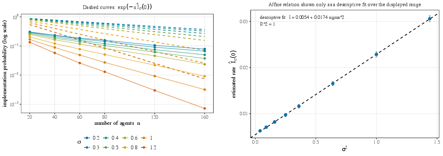
10.3 Hierarchical Unknown-Endpoint Diagnostic↩︎
The hierarchical theorem assumes a common conditional support. The numerical specification \[X_i\mid\theta\sim\mathop{\mathrm{Unif}}[\underline{x},\theta]\] instead has a parameter-dependent support and is nonregular, so it falls outside Theorem 3 (Remark 9). It is included only as a descriptive diagnostic.
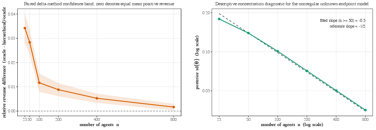
10.4 Equal-Scale Welfare–Revenue Frontiers↩︎
At equal scale, Laplace Blackwell-dominates logistic (Proposition 5). Both the maximal reduced-form revenue and the full reduced-form welfare–revenue frontier are therefore weakly higher under Laplace.
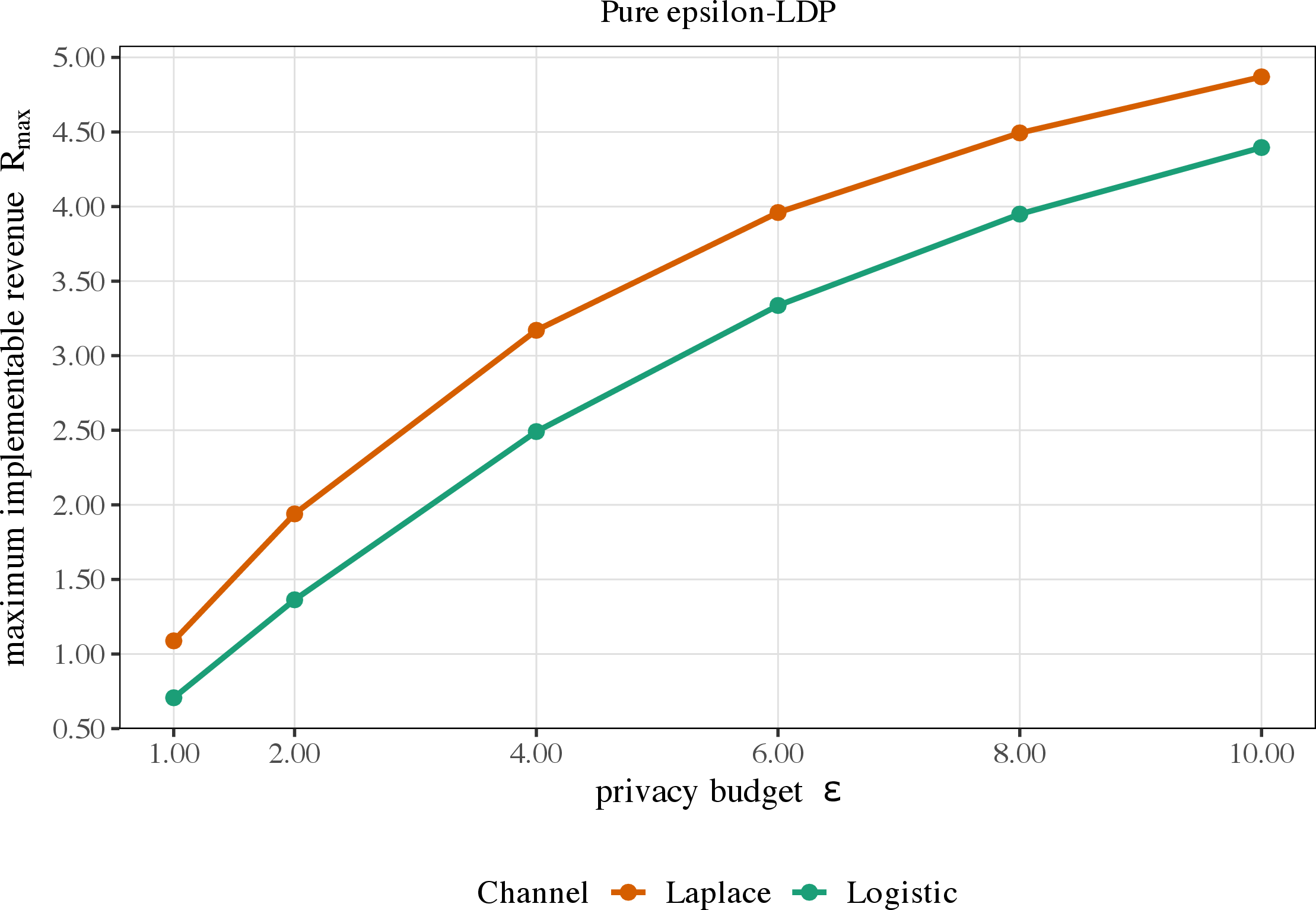
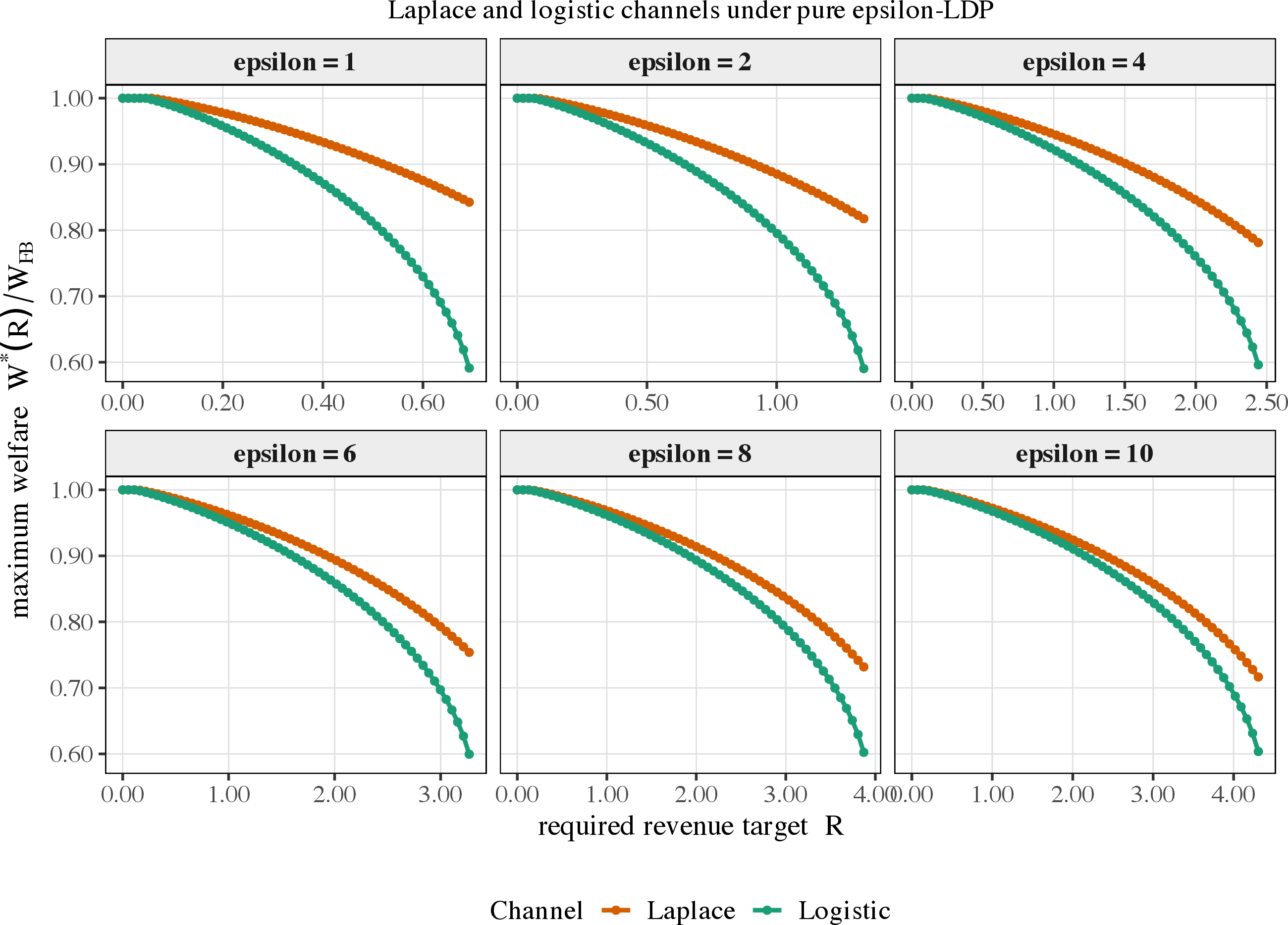
10.5 Common-\(\mu\) Endpoint and Continuous-Type Comparisons↩︎
The left panel of Figure 10 displays the exact endpoint trade-off difference \[\mathcal{T}_{\mathrm{Lap}}(\alpha) - \mathcal{T}_{\mathrm{Log}}(\alpha),\] which is nonnegative by Theorem 4 and vanishes at \[\alpha\in\{0,\Phi(-\mu/2),1\},\] the three testing levels at which both endpoint experiments touch the Gaussian benchmark (Remark 13).
The right panel reports the corresponding continuous-type welfare difference. That difference is a numerical quantity, not a consequence of the endpoint Blackwell theorem. Its confidence band overlaps zero over a substantial part of the displayed range, so the simulation does not support extending the endpoint Blackwell order to the full continuum (Remark 12).
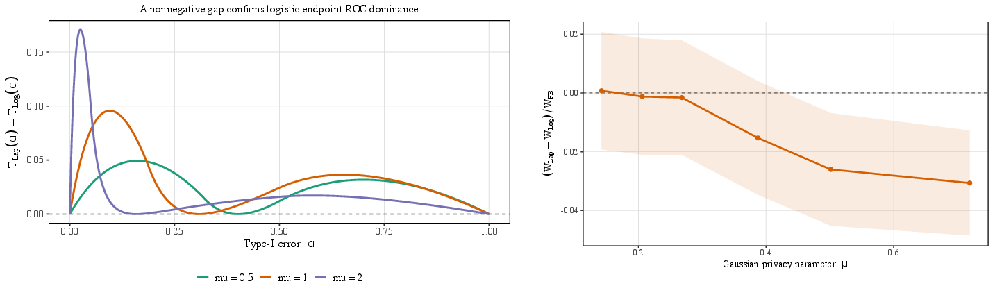
10.6 Welfare–Revenue Trade-off under Approximate LDP↩︎
This experiment uses a common \((\epsilon,\delta)\)-LDP frontier with \[\delta=10^{-5},\] under the prior \(X\sim\mathop{\mathrm{Unif}}[-0.5,1.5]\) of the design section. The first panel reports welfare efficiency against the privacy budget. The second reports welfare and signed reduced-form revenue as the score multiplier varies, with the vertical reference at the mean-score boundary \(\lambda_{\mathrm{crit}}=1\).
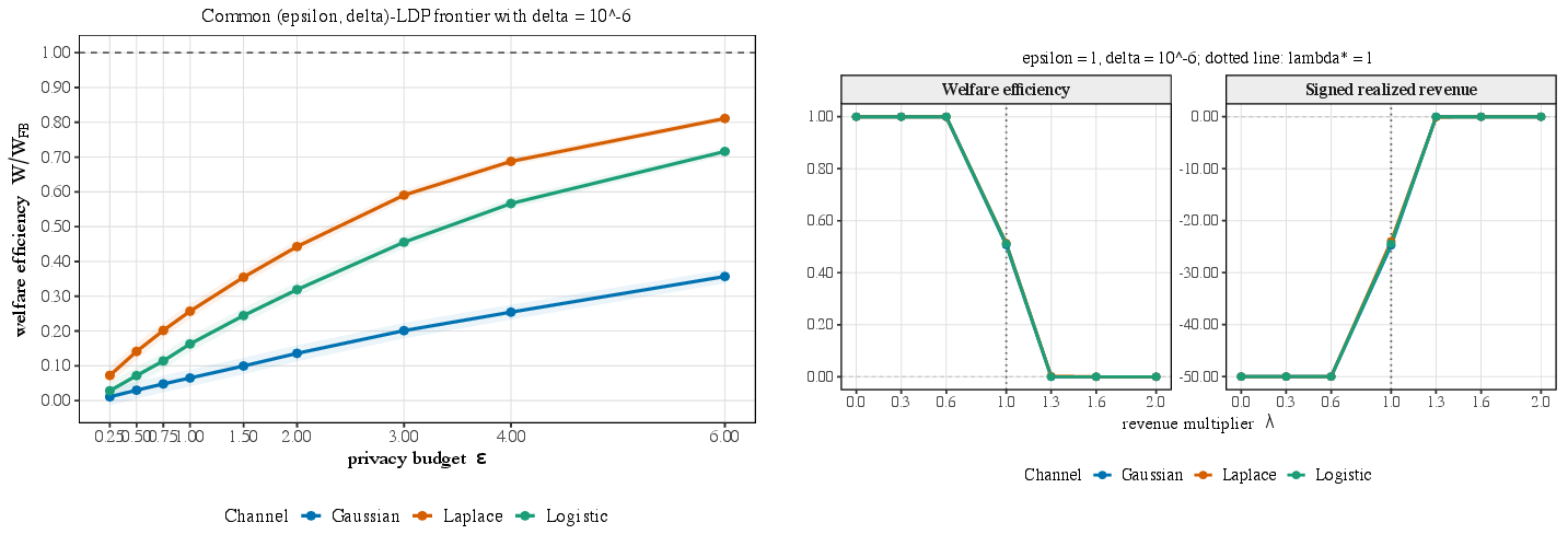
Online Supplement
Public Good Provision under Locally Private Signals
Scope of the Supplement↩︎
This supplement collects the technical material, clarifications, and numerical details accompanying the main paper. Its principal purpose is to make precise the distinction among three objects that are easy to conflate.
The reduced-form allocation problem, in which Bayesian incentive compatibility is expressed through interim monotonicity and the envelope formula.
Exact signal-measurable implementation, which additionally requires the envelope-prescribed interim transfer to lie in the range of the channel’s conditional-expectation operator.
Approximate signal-measurable implementation, obtained when the implementing Fredholm equation is solved only up to a controlled residual.
The main paper gives a sharp characterization of the optimal reduced-form allocation and the corresponding reduced-form revenue envelope. Exact Bayesian implementation by transfers measurable with respect to the privatized signals is conditional on a Fredholm range condition, which need not hold automatically for smoothing channels. This supplement therefore provides both an exact range characterization and a quantitative approximate-implementation theorem that converts a Fredholm residual into explicit incentive, participation, and revenue errors.
The supplement also supplies the revelation argument appropriate to the privacy-channel environment, explains the lowest-type participation normalization, delimits the scope of completeness, records the precise status of the hierarchical extension, and documents the complete numerical methodology. In particular, no ironing argument is required for the Laplace channel: weak MLRP preserves weak monotonicity, and the flat posterior-score tails create pooling without violating Bayesian incentive compatibility.
Throughout, \(\mathcal{X}=[\underline{x},\bar{x}]\) is the bounded type space, \(K\) the privacy channel with conditional density \(k(y\mid x)\), and all expectations are taken under the truthful signal law. Cross-references prefixed “M-” point to the main paper.
11 Exact Reduced-Form BIC and Signal-Measurable Implementation↩︎
11.1 The conditional-expectation operator↩︎
Fix an agent \(i\). Once the allocation rule \(q\) is selected, the envelope formula determines the target interim transfer \[\label{supp:eq95target95transfer} T_i^{q}(x) = xQ_i^{q}(x) - \int_{\underline{x}}^{x}Q_i^{q}(z)\,dz,\tag{94}\] where the interim allocation is \[\label{supp:eq95interim95allocation} Q_i^{q}(x) = \int_{\mathcal{Y}^n} q(y)\, k(y_i\mid x)\, f_{Y_{-i}}(y_{-i})\,dy.\tag{95}\]
For any signal-measurable ex-post transfer \(t_i:\mathcal{Y}^n\to\mathbb{R}\), define its opponent average under the truthful law \[\label{supp:eq95opponent95average} g_i(y_i) = \int_{\mathcal{Y}^{n-1}} t_i(y_i,y_{-i})\, f_{Y_{-i}}(y_{-i})\,dy_{-i}.\tag{96}\] In the notation of the main paper, \(g_i\) is the opponent-averaged transfer \(\bar t_i\). The induced interim transfer depends on \(t_i\) only through \(g_i\), through the conditional-expectation operator \[\label{supp:eq95operator} (\mathcal{K} g_i)(x) := \int_{\mathcal{Y}} g_i(y)\,k(y\mid x)\,dy = \mathbb{E}[g_i(Y_i)\mid X_i=x].\tag{97}\] Exact signal-measurable implementation therefore requires \[\label{supp:eq95exact95range} \mathcal{K} g_i = T_i^{q}.\tag{98}\] Equation 98 is a Fredholm integral equation of the first kind; it is the equation stated in the main paper, with \(T_i^{q}\) the required interim payment.
Proposition 18 (Exact implementation is a range condition). Fix an allocation rule \(q\) whose interim allocation \(Q_i^{q}\) is weakly increasing, and let \(T_i^{q}\) be given by 94 . The following are equivalent.
There exists an integrable signal-measurable transfer \(t_i:\mathcal{Y}^n\to\mathbb{R}\) that implements the envelope interim transfer \(T_i^{q}\).
There exists an integrable \(g_i:\mathcal{Y}\to\mathbb{R}\) with \(\mathcal{K} g_i=T_i^{q}\).
\(T_i^{q}\in\mathop{\mathrm{Ran}}(\mathcal{K})\).
Whenever \(g_i\) solves the one-dimensional equation, the transfer \(t_i(y_i,y_{-i})=g_i(y_i)\) is an exact signal-measurable implementation.
Proof. If \(t_i\) implements \(T_i^{q}\), its opponent average \(g_i\) from 96 satisfies \(T_i^{q}(x)=\int_\mathcal{Y}g_i(y)k(y\mid x)\,dy=(\mathcal{K} g_i)(x)\), giving (i)\(\Rightarrow\)(ii). The equivalence (ii)\(\Leftrightarrow\)(iii) is the definition of the range. Finally, if \(g_i\) solves the one-dimensional equation, then with \(t_i(y)=g_i(y_i)\), \[\mathbb{E}[t_i(Y)\mid X_i=x] = \mathbb{E}[g_i(Y_i)\mid X_i=x] = (\mathcal{K} g_i)(x) = T_i^{q}(x),\] which gives (ii)\(\Rightarrow\)(i). ◻
Remark 16 (What exact BIC means in the paper). The reduced-form allocation characterized in the main paper is exactly BIC in the standard one-dimensional reduced-form sense: its interim allocation is monotone, and the envelope formula gives the unique normalized interim transfer. The stronger statement that the reduced form is implemented by transfers measurable with respect to the privatized signals requires Proposition 18. References to an “exactly implementable mechanism” are therefore always conditional on \(T_i^{q}\in\mathop{\mathrm{Ran}}(\mathcal{K})\).
11.2 Why smoothing creates a genuine implementation problem↩︎
For Gaussian and other smoothing kernels, \(\mathcal{K}\) maps functions of the signal into smoother functions of the type. When the operator is considered on Hilbert spaces for which its kernel is square integrable—for example, after restriction to compact type and signal domains, or under appropriate weighted \(L^2\) conditions—it is a Hilbert–Schmidt operator and hence compact. More generally, smoothing channel operators often have nonclosed range and unstable inversion, but compactness must be verified for the particular function spaces used. Whenever \(\mathcal{K}\) is compact and injective on an infinite-dimensional domain, its range cannot be both infinite dimensional and closed; its inverse on the range is therefore unbounded, and solving \(\mathcal{K} g=T\) is ill posed.
This has two distinct implications.
Uniqueness does not imply existence. Completeness can make \(\mathcal{K}\) injective, but injectivity only says two exact solutions cannot differ; it does not produce a solution for a prescribed target.
Numerical regularization does not prove exact implementation. A small finite-grid residual shows that a discretized target is well approximated on that grid. It does not establish that the continuous target lies in the continuous operator range.
The main paper therefore interprets its Fredholm numerical experiment as an approximation-and-conditioning diagnostic rather than as a proof of exact range membership.
11.3 A nontrivial exact-implementation class↩︎
Although a generic target need not lie in the range of a smoothing operator, the range is neither empty nor economically trivial. For additive channels, polynomial interim transfers admit exact signal-measurable implementations.
Proposition 19 (Polynomial targets under additive noise). Suppose \(Y=X+\varepsilon\), where \(\varepsilon\) is independent of \(X\) with finite moments through order \(m\), and let \((\mathcal{K} g)(x)=\mathbb{E}[g(x+\varepsilon)]\). Then, restricted to polynomials of degree at most \(m\), \(\mathcal{K}\) is a bijection. In particular, for every \(T(x)=\sum_{r=0}^{m}a_rx^r\) there is a unique polynomial \(g(y)=\sum_{r=0}^{m}b_ry^r\) of degree at most \(m\) with \(\mathbb{E}[g(x+\varepsilon)]=T(x)\) for all \(x\in\mathbb{R}\).
Proof. For each \(r\le m\), \[\mathbb{E}[(x+\varepsilon)^r] = \sum_{\ell=0}^{r} \binom{r}{\ell} x^{r-\ell}\, \mathbb{E}[\varepsilon^\ell],\] so \(\mathcal{K}\) sends the monomial \(y^r\) to a degree-\(r\) polynomial in \(x\) with leading coefficient one. In the monomial basis \((1,x,\ldots,x^m)\) the matrix of this map is upper triangular with unit diagonal, hence invertible. Every degree-\(\le m\) target thus has a unique degree-\(\le m\) preimage. ◻
The uniqueness asserted here is uniqueness within the finite-dimensional space of polynomials of degree at most \(m\). Uniqueness among all admissible transfers additionally requires injectivity of the channel operator on the maintained transfer space.
Corollary 9 (Affine interim allocations). If the additive channel has finite second moment and the interim allocation is affine, \(Q_i(x)=a_ix+b_i\), then the normalized envelope transfer is the quadratic \[T_i(x) = xQ_i(x)-\int_{\underline{x}}^{x}Q_i(z)\,dz = \frac{a_i}{2}x^2 + \frac{a_i}{2}\underline{x}^2 + b_i\underline{x},\] which has an exact signal-measurable implementation.
Proof. Direct integration gives \[T_i(x) = a_ix^2+b_ix - \frac{a_i}{2}(x^2-\underline{x}^2) - b_i(x-\underline{x}) = \frac{a_i}{2}x^2+\frac{a_i}{2}\underline{x}^2+b_i\underline{x},\] a polynomial of degree at most two; apply Proposition 19. ◻
Example 3 (Explicit quadratic implementation). Let \(Y=X+\varepsilon\) with \(\mathbb{E}[\varepsilon]=0\) and \(\mathop{\mathrm{Var}}(\varepsilon)=\sigma_\varepsilon^2\). If \(T(x)=c_2x^2+c_1x+c_0\), then \[g(y)=c_2\bigl(y^2-\sigma_\varepsilon^2\bigr)+c_1y+c_0\] satisfies \(\mathbb{E}[g(Y)\mid X=x]=T(x)\). This covers centered Gaussian, Laplace, and logistic additive noise.
11.4 Approximate signal-measurable implementation↩︎
When the target does not belong to \(\mathop{\mathrm{Ran}}(\mathcal{K})\), or when range membership is unknown, the economically relevant question is how a Fredholm approximation error translates into incentive and participation errors.
Definition 3 (Uniform Fredholm residual). Let \(T_i^{q}\) be the normalized envelope transfer associated with a monotone interim allocation \(Q_i^{q}\). An opponent-averaged transfer \(g_i\) has uniform Fredholm residual at most \(\eta_i\) if \[\label{supp:eq95uniform95residual} \sup_{x\in\mathcal{X}} \bigl| (\mathcal{K} g_i)(x)-T_i^{q}(x) \bigr| \le \eta_i.\tag{99}\]
Write \(\widetilde{T}_i(x)=(\mathcal{K} g_i)(x)\) for the induced interim transfer and \(e_i(x)=\widetilde{T}_i(x)-T_i^{q}(x)\) for the pointwise error.
Theorem 6 (Fredholm residual implies approximate BIC and IR). Let \(Q_i:\mathcal{X}\to[0,1]\) be weakly increasing, let \(T_i(x)=xQ_i(x)-\int_{\underline{x}}^{x}Q_i(z)\,dz\), and suppose \(g_i:\mathcal{Y}\to\mathbb{R}\) satisfies \(\sup_{x\in\mathcal{X}}|(\mathcal{K} g_i)(x)-T_i(x)|\le\eta_i\). Use the signal-measurable transfer \(t_i(y)=g_i(y_i)\). Then:
the mechanism is \(2\eta_i\)-BIC for agent \(i\), \[\label{supp:eq95approx95bic} xQ_i(x)-\widetilde{T}_i(x) \ge xQ_i(z)-\widetilde{T}_i(z)-2\eta_i \qquad \forall x,z\in\mathcal{X};\tag{100}\]
the mechanism is \(\eta_i\)-interim individually rational, \[\label{supp:eq95approx95ir} xQ_i(x)-\widetilde{T}_i(x)\ge-\eta_i \qquad \forall x\in\mathcal{X};\tag{101}\]
the expected-transfer error satisfies \(\bigl|\mathbb{E}[\widetilde{T}_i(X_i)]-\mathbb{E}[T_i(X_i)]\bigr|\le\eta_i\), so that for \(n\) agents \[\label{supp:eq95revenue95error} \Bigl| \mathbb{E}\!\Bigl[\textstyle\sum_{i=1}^{n}\widetilde{T}_i(X_i)\Bigr] - \mathbb{E}\!\Bigl[\textstyle\sum_{i=1}^{n}T_i(X_i)\Bigr] \Bigr| \le \sum_{i=1}^{n}\eta_i,\tag{102}\] which is at most \(n\eta\) when \(\eta_i\le\eta\) for every \(i\).
Proof. The exact envelope pair \((Q_i,T_i)\) is BIC, so \(xQ_i(x)-T_i(x)\ge xQ_i(z)-T_i(z)\) for all \(x,z\). Since \(\widetilde{T}_i=T_i+e_i\) with \(|e_i|\le\eta_i\), \[\begin{align} xQ_i(x)-\widetilde{T}_i(x) &= xQ_i(x)-T_i(x)-e_i(x) \ge xQ_i(z)-T_i(z)-e_i(x) \\ &= xQ_i(z)-\widetilde{T}_i(z)+e_i(z)-e_i(x) \ge xQ_i(z)-\widetilde{T}_i(z)-2\eta_i, \end{align}\] proving (i). Under \(U_i(\underline{x})=0\), exact BIC gives \(U_i(x)=\int_{\underline{x}}^{x}Q_i(s)\,ds\ge0\), so \(xQ_i(x)-\widetilde{T}_i(x)=U_i(x)-e_i(x)\ge-\eta_i\), proving (ii). Finally \(|\mathbb{E}[\widetilde{T}_i(X_i)-T_i(X_i)]|=|\mathbb{E}[e_i(X_i)]|\le\mathbb{E}|e_i(X_i)|\le\eta_i\), and summing gives 102 . ◻
Corollary 10 (Exact implementation as the zero-residual case). If \(\eta_i=0\), Theorem 6 yields exact BIC, exact interim IR, and exact reduced-form revenue.
Remark 17 (Norm choice). The uniform residual is used because it yields type-uniform incentive and participation bounds. An \(L^2(F)\) residual controls average transfer error but does not, without further regularity, give a uniform BIC bound over all type–report pairs. A numerical procedure should therefore report both its weighted least-squares residual and a dense-grid approximation to \(\sup_{x\in\mathcal{X}}|(\mathcal{K} g_i)(x)-T_i(x)|\).
11.5 Regularization and the meaning of the numerical solution↩︎
A common numerical estimator is the Tikhonov solution \[\label{supp:eq95tikhonov} g_{\alpha} \in \mathop{\mathrm{arg\,min}}_{g\in\mathcal{G}} \Bigl\{ \|\mathcal{K} g-T\|_{\mathcal{H}_X}^{2} + \alpha\|g\|_{\mathcal{H}_Y}^{2} \Bigr\},\tag{103}\] with regularization parameter \(\alpha>0\) and chosen spaces \(\mathcal{H}_X,\mathcal{H}_Y\). The role of \(\alpha\) is stability, not exact implementation: for \(\alpha>0\) the residual generally does not vanish even when an exact solution exists, and a small discretized residual need not place the continuous target in the exact range.
Proposition 20 (Economic interpretation of a regularized solution). If a regularized solution \(g_\alpha\) satisfies \(\sup_{x\in\mathcal{X}}|(\mathcal{K} g_\alpha)(x)-T(x)|\le\eta_\alpha\), then the mechanism \(t_i^\alpha(y)=g_\alpha(y_i)\) is \(2\eta_\alpha\)-BIC and \(\eta_\alpha\)-IR, with per-agent expected-revenue error at most \(\eta_\alpha\). The economically meaningful output is therefore the uniform residual \(\eta_\alpha\), not the condition number or the positivity of the discretized singular values.
Proof. Apply Theorem 6. ◻
12 Revelation through an Exogenous Privacy Channel↩︎
The strategic action of agent \(i\) is not the realized signal \(Y_i\), generated by the exogenous channel, but the submitted report \(r_i\in\mathcal{X}\). A signal-measurable mechanism \((q,t)\) induces, for each submission \(r_i\) and given truthful opponents, the interim schedules \[\label{supp:eq95submission95reduced95form} Q_i(r_i)=\mathbb{E}[q(Y)\mid R_i=r_i], \qquad T_i(r_i)=\mathbb{E}[t_i(Y)\mid R_i=r_i],\tag{104}\] and a true type \(x_i\) submitting \(r_i\) obtains \[\label{supp:eq95submission95utility} u_i(x_i,r_i)=x_iQ_i(r_i)-T_i(r_i).\tag{105}\] All strategic comparisons are summarized by the one-dimensional menu \(r_i\mapsto(Q_i(r_i),T_i(r_i))\).
Proposition 21 (Channel-induced taxation principle). Fix the opponents’ truthful strategy and the distribution of their signals. Every signal-measurable mechanism induces a one-dimensional menu \(\{(Q_i(r),T_i(r)):r\in\mathcal{X}\}\), and truthful submission is Bayesian optimal if and only if \[\label{supp:eq95channel95bic} xQ_i(x)-T_i(x) \ge xQ_i(r)-T_i(r) \qquad \forall x,r\in\mathcal{X}.\qquad{(21)}\] Hence the usual one-dimensional envelope characterization applies to the channel-induced reduced form. Conversely, a monotone reduced-form pair \((Q_i,T_i)\) is implementable by the original privacy-channel mechanism only if there is a signal-measurable allocation and transfer whose conditional expectations equal \(Q_i\) and \(T_i\).
Proof. Conditional on \(r_i\), the agent cannot affect the realized channel noise, so expected utility is exactly 105 and truthfulness is optimal precisely when ?? holds. The standard one-dimensional incentive argument then forces \(Q_i\) weakly increasing and the envelope identity. The converse separates abstract reduced-form implementability from implementation through the given kernel. ◻
Remark 18 (No direct revelation of the privatized signal). The planner does not ask the agent to report \(Y_i\). The local randomizer produces \(Y_i\) after the agent selects \(r_i\), and the realized signal is observed only by the planner. The directness of the mechanism refers to the submitted channel input \(r_i\), not to control of the random output.
13 Why Interim IR Binds at the Lowest Type↩︎
For weakly increasing nonnegative \(Q_i\), BIC gives \(U_i(x)=U_i(\underline{x})+\int_{\underline{x}}^{x}Q_i(s)\,ds\ge U_i(\underline{x})\), so interim IR is equivalent to \(U_i(\underline{x})\ge0\).
Proposition 22 (Revenue-maximizing IR normalization). Fix a BIC interim allocation \(Q_i\). Among all interim transfer schedules implementing \(Q_i\) and satisfying interim IR, expected revenue is maximized by \(U_i(\underline{x})=0\). This holds regardless of the sign of \(\underline{x}\).
Proof. Every BIC transfer implementing \(Q_i\) has the form \(T_i(x)=xQ_i(x)-U_i(\underline{x})-\int_{\underline{x}}^{x}Q_i(s)\,ds\). Interim IR requires \(U_i(\underline{x})\ge0\), and raising \(U_i(\underline{x})\) subtracts the same positive constant from every type’s transfer, lowering expected revenue one-for-one. Hence \(U_i(\underline{x})=0\) is revenue-maximizing. The argument uses only \(Q_i\ge0\), so utility is minimized at the lowest type irrespective of the sign of \(\underline{x}\). ◻
14 Completeness: What Can Be Claimed↩︎
14.1 Injectivity and uniqueness↩︎
The completeness assumption in the main paper is an injectivity condition for \(\mathcal{K} g(x)=\int_\mathcal{Y}g(y)k(y\mid x)\,dy\): if \(\mathcal{K} g\equiv0\) on \(\mathcal{X}\) implies \(g=0\) a.e., then two opponent-averaged transfers implementing the same interim schedule coincide. This is a uniqueness statement only; it does not assert \(\mathop{\mathrm{Ran}}(\mathcal{K})\) equals the entire target space.
14.2 The Fourier condition for full location families↩︎
For an additive channel \(Y=X+\varepsilon\) with noise density \(h\), \((\mathcal{K} g)(x)=\int_\mathbb{R}g(y)h(y-x)\,dy\), which up to reflection is convolution.
Proposition 23 (Fourier injectivity on the full location family). Let \(g\in L^1(\mathbb{R})\), \(h\in L^1(\mathbb{R})\), and suppose the characteristic function \(\widehat h(t)=\int_\mathbb{R}e^{ity}h(y)\,dy\) is nowhere zero. If \((g*\widetilde{h})(x)=0\) for a.e.\(x\in\mathbb{R}\), where \(\widetilde{h}(u)=h(-u)\), then \(g=0\) a.e.
Proof. Taking Fourier transforms gives \(\widehat g(t)\,\widehat{\widetilde{h}}(t)=0\) for all \(t\). Since \(\widehat{\widetilde{h}}(t)=\overline{\widehat h(t)}\ne0\), we get \(\widehat g\equiv0\), and uniqueness of the Fourier transform on \(L^1(\mathbb{R})\) gives \(g=0\) a.e. ◻
The centered Gaussian, Laplace, and logistic characteristic functions are \[\widehat h_{\mathrm G}(t)=e^{-\sigma^2t^2/2}, \qquad \widehat h_{\mathrm{Lap}}(t)=\frac{1}{1+b^2t^2}, \qquad \widehat h_{\mathrm{Log}}(t)=\frac{\pi\beta t}{\sinh(\pi\beta t)},\] with the logistic value extended continuously to one at \(t=0\). None vanishes on \(\mathbb{R}\), so the corresponding full location families are injective on \(L^1(\mathbb{R})\).
14.3 Why a compact type interval requires care↩︎
The main model indexes the family only by \(x\in[\underline{x},\bar{x}]\). Knowing \((\mathcal{K} g)(x)=0\) for \(x\in[\underline{x},\bar{x}]\) only is weaker than knowing the convolution vanishes for every \(x\in\mathbb{R}\), and the nowhere-vanishing characteristic-function argument alone does not bridge this gap.
For the Gaussian kernel, additional analyticity supplies unique continuation: the Gaussian convolution is real analytic under standard integrability bounds, so vanishing on a nonempty interval forces vanishing everywhere, after which Fourier injectivity gives \(g=0\). For Laplace and logistic kernels, completeness over a compact parameter interval depends on the function class and on additional continuation properties. The paper therefore does not infer compact-interval completeness from the characteristic function alone; it states completeness as an assumption wherever compact-interval uniqueness is needed.
Remark 19 (Correct interpretation). Keep separate: (i) a nowhere-vanishing characteristic function gives injectivity for the full additive location family on standard convolution spaces; (ii) Gaussian analyticity can extend interval-wise vanishing to global vanishing under suitable integrability; (iii) compact-interval completeness for a particular channel and function space needs its own verification; and (iv) none of these injectivity statements implies surjectivity or exact range membership.
15 The Hierarchical Extension: Exact Scope↩︎
With a latent common parameter \(\theta\), the hierarchical posterior score \[\Psi_i(y,\lambda) = \mathbb{E}_{\theta\mid y} \!\bigl[ \widehat x^\theta(y_i)+\lambda\widehat J^\theta(y_i) \bigr]\] depends on the entire signal vector through the posterior \(p(\theta\mid y)\). Changing \(y_i\) moves both the conditional posterior of \(X_i\) and the posterior of \(\theta\). Consequently, MLRP of the individual channel does not by itself make \(y_i\mapsto\sum_{j}\Psi_j(y,\lambda)\) increasing.
15.1 The high-level monotonicity condition↩︎
The main hierarchical theorem assumes coordinatewise monotonicity of the aggregate hierarchical score. This is sufficient for the acceptance region to be an upper set in every signal coordinate; conditional MLRP then makes every \(\theta\)-conditional interim allocation monotone. The condition is not claimed to be primitive: an increase in one signal can move the common-state posterior in a way that lowers other agents’ posterior virtual values.
Remark 20 (What the hierarchical theorem resolves). Conditional on coordinatewise score monotonicity, the theorem provides (i) the posterior-score Lagrangian, (ii) the pointwise threshold structure, (iii) conditional reduced-form BIC, (iv) the family of conditional Fredholm equations, and (v) the hierarchical reduced-form revenue representation and complementary slackness condition. It does not give a primitive characterization of when coordinatewise monotonicity holds, nor of Crémer–McLean extraction under privatized common-state signals.
15.2 A primitive sufficient condition↩︎
Proposition 24 (A sufficient derivative condition). For \(j=1,\ldots,n\), define \[a_j^\theta(y_j,\lambda) = \widehat x^\theta(y_j)+\lambda\widehat J^\theta(y_j).\] Suppose the aggregate hierarchical score is differentiable in each signal coordinate and the required differentiation-under-the-integral and dominated-derivative conditions hold. If, for every \(i\), \(y\), and \(\lambda\ge0\), \[\label{supp:eq95hierarchical95derivative95condition} \mathbb{E}_{\theta\mid y} \!\left[ \frac{\partial}{\partial y_i} a_i^\theta(y_i,\lambda) \right] + \mathop{\mathrm{Cov}}_{\theta\mid y} \!\left( \sum_{j=1}^{n}a_j^\theta(y_j,\lambda),\, \frac{\partial}{\partial y_i}\log p(\theta\mid y) \right) \ge0,\qquad{(22)}\] then the aggregate hierarchical score is coordinatewise weakly increasing, and the hierarchical threshold allocation induces weakly increasing conditional interim allocations. Equivalently, the covariance term in ?? may be written as \[\sum_{j=1}^{n} \mathop{\mathrm{Cov}}_{\theta\mid y} \!\left( a_j^\theta(y_j,\lambda),\, \frac{\partial}{\partial y_i}\log p(\theta\mid y) \right).\]
Proof. The aggregate hierarchical score is \[G_\lambda^{\mathrm H}(y) = \sum_{j=1}^{n} \mathbb{E}_{\theta\mid y} \!\left[a_j^\theta(y_j,\lambda)\right].\] For a posterior expectation of a \(y\)-dependent integrand \(a_\theta(y)\), the score-function identity gives \[\frac{\partial}{\partial y_i} \mathbb{E}_{\theta\mid y}[a_\theta(y)] = \mathbb{E}_{\theta\mid y} \!\left[\frac{\partial a_\theta(y)}{\partial y_i}\right] + \mathop{\mathrm{Cov}}_{\theta\mid y} \!\left( a_\theta(y),\, \frac{\partial}{\partial y_i}\log p(\theta\mid y) \right),\] because \(\mathbb{E}_{\theta\mid y}\!\left[\frac{\partial}{\partial y_i}\log p(\theta\mid y)\right]=0\). For \(j\ne i\), the integrand \(a_j^\theta(y_j,\lambda)\) has no direct dependence on \(y_i\), so its \(\mathbb{E}_{\theta\mid y}[\partial_{y_i}\,\cdot\,]\) contribution vanishes and only its covariance term survives. Summing over \(j\), \[\frac{\partial}{\partial y_i} G_\lambda^{\mathrm H}(y) = \mathbb{E}_{\theta\mid y} \!\left[\frac{\partial}{\partial y_i}a_i^\theta(y_i,\lambda)\right] + \mathop{\mathrm{Cov}}_{\theta\mid y} \!\left( \sum_{j=1}^{n}a_j^\theta(y_j,\lambda),\, \frac{\partial}{\partial y_i}\log p(\theta\mid y) \right).\] Condition ?? therefore gives \(\partial G_\lambda^{\mathrm H}/\partial y_i\ge0\) for every \(i\), proving coordinatewise weak monotonicity. Conditional MLRP then yields weakly increasing conditional interim allocations. ◻
The covariance term is the source of the difficulty. It vanishes under a known prior and under a degenerate meta-prior, but is generally nonzero in a genuine hierarchical model.
15.3 The unknown-endpoint simulation↩︎
The hierarchical numerical experiment uses supports of the form \([\,0.3,\theta\,]\). This violates the common-support assumption of the formal theorem and is included as a numerical extension, not a verification of it. Because \(\theta\) is a support endpoint, the model is nonregular before convolution, and privacy convolution changes the identification and concentration problem. The supplement therefore reports the observed posterior contraction descriptively and does not invoke an unproved Bernstein–von Mises theorem.
16 Revenue Envelopes and Economic Interpretation↩︎
16.1 Reduced-form revenue versus implementable revenue↩︎
For the known-prior model, let \(V_n(Y)=\sum_{i=1}^{n}\widehat J_i(Y_i)\). The maximum reduced-form revenue is \[R_n^{*,\mathrm{red}}(K)=\mathbb{E}[(V_n(Y))_+],\] which is exact for the reduced-form problem because the pointwise revenue-maximizing allocation is \(q^{\mathrm{rev}}(Y)=\mathbf{1}\{V_n(Y)>0\}\), with an arbitrary value on the null tie set \(\{V_n=0\}\). Let \(R_n^{*,\mathrm{sig}}(K)\) be the maximum revenue among mechanisms whose allocation and transfers are signal-measurable and satisfy exact BIC and interim IR. Then \[\label{supp:eq95revenue95upper95bound} R_n^{*,\mathrm{sig}}(K)\le R_n^{*,\mathrm{red}}(K),\tag{106}\] Equality holds if a reduced-form revenue maximizer has envelope transfers belonging to the relevant Fredholm ranges. Conversely, if the reduced-form revenue maximizer is unique up to truthful-law almost-sure equality, then equality in 106 requires that maximizer to admit signal-measurable transfer implementation.
Corollary 11 (Approximate revenue attainability). If the revenue-maximizing reduced form has envelope transfers \(T_i^{\mathrm{rev}}\) and, for every \(i\), there is \(g_i\) with \(\sup_{x\in\mathcal{X}}|\mathcal{K} g_i(x)-T_i^{\mathrm{rev}}(x)|\le\eta_i\), then there is a signal-measurable mechanism that is \(2\eta_i\)-BIC and \(\eta_i\)-IR for each agent and whose expected revenue is within \(\sum_i\eta_i\) of \(R_n^{*,\mathrm{red}}(K)\).
Proof. Apply Theorem 6 to each agent’s envelope target. ◻
16.2 The large-deviation rate function↩︎
The negative-drift regime below is stated through the Cramér rate function of the per-agent posterior virtual value. We define this object precisely before using it.
Set \[\label{supp:eq95Z95def} Z_i=\widehat J_i(Y_i), \qquad S_n=\sum_{i=1}^{n}Z_i.\tag{107}\] Under the regularity and MLRP assumptions of the main paper, \(\widehat J_i(Y_i)\) is bounded, say \(|Z_i|\le M\), and the \(Z_i\) are i.i.d.with common mean \[\label{supp:eq95Z95mean} \mathbb{E}[Z_i]=\mathbb{E}[\widehat J_i(Y_i)]=\underline{x},\tag{108}\] the lower-endpoint identity of the main paper.
Definition 4 (Cumulant generating function and Cramér rate). The cumulant generating function (log moment generating function) of \(Z_1\) is \[\label{supp:eq95cgf} \Lambda(t)=\log\mathbb{E}\!\bigl[e^{tZ_1}\bigr], \qquad t\in\mathbb{R},\tag{109}\] which is finite for all \(t\in\mathbb{R}\) because \(Z_1\) is bounded. The associated Cramér rate function is its Legendre–Fenchel transform \[\label{supp:eq95rate95function} I_K(a)=\sup_{t\in\mathbb{R}}\bigl\{ta-\Lambda(t)\bigr\}, \qquad a\in\mathbb{R}.\tag{110}\]
The function \(I_K\) is convex, lower semicontinuous, and nonnegative, with \(I_K(\mathbb{E}[Z_1])=I_K(\underline{x})=0\) (the supremum in 110 at \(a=\underline{x}\) is attained at \(t=0\), since \(\Lambda'(0)=\mathbb{E}[Z_1]=\underline{x}\)). Because \(\Lambda\) is convex with \(\Lambda(0)=0\) and \(\Lambda'(0)=\underline{x}\), the value at \(a=0\) specializes to \[\label{supp:eq95rate95at95zero} I_K(0)=\sup_{t\in\mathbb{R}}\bigl\{-\Lambda(t)\bigr\}=-\inf_{t\in\mathbb{R}}\Lambda(t).\tag{111}\] If \(\underline{x}<0\) and \(0\) lies in the interior of the convex hull of \(\mathop{\mathrm{supp}}(Z_1)\), then the tilting equation \(\Lambda'(t^*)=0\) has a solution \(t^*>0\), and \[\label{supp:eq95rate95positive} I_K(0)=-\Lambda(t^*)>0,\tag{112}\] strictly positive because \(\Lambda\) is strictly decreasing at \(t=0\) (\(\Lambda'(0)=\underline{x}<0\)), so \(\inf_t\Lambda(t)<\Lambda(0)=0\).
Lemma 20 (Cramér rate for the build event). Suppose \(\underline{x}<0\) and \(0\) lies in the interior of the convex hull of \(\mathop{\mathrm{supp}}(Z_1)\). Then \[\label{supp:eq95cramer95limit} \lim_{n\to\infty}\frac{1}{n}\log\mathbb{P}\!\left(\frac{S_n}{n}\ge0\right) = -\,\inf_{a\ge0}I_K(a) = -\,I_K(0),\tag{113}\] with \(I_K(0)\) given by 111 –112 .
Proof. Cramér’s theorem for i.i.d.bounded summands gives \(\lim_n\frac{1}{n}\log\mathbb{P}(S_n/n\ge0)=-\inf_{a\ge0}I_K(a)\). The function \(I_K\) is convex with unique minimizer \(a=\underline{x}\) (value zero) and is nondecreasing on \([\underline{x},\infty)\). Since \(0>\underline{x}\), the infimum over \(a\ge0\) is attained at \(a=0\), giving \(-I_K(0)\). Positivity of \(I_K(0)\) is 112 . ◻
16.3 The three regimes↩︎
Using Definition 4, the known-prior reduced-form theorem gives the following behavior of \(R_n^{*,\mathrm{red}}(K)=\mathbb{E}[(S_n)_+]\), with \(\sigma_J(K)^2=\mathop{\mathrm{Var}}(Z_1)\in(0,\infty)\).
If \(\underline{x}>0\), then \(R_n^{*,\mathrm{red}}(K)=n\underline{x}+o(n)\); more precisely the remainder is exponentially small.
If \(\underline{x}=0\), then \(R_n^{*,\mathrm{red}}(K)=\dfrac{\sigma_J(K)}{\sqrt{2\pi}}\sqrt n+o(\sqrt n)\).
If \(\underline{x}<0\) and \(0\) lies in the interior of the convex hull of \(\mathop{\mathrm{supp}}(Z_1)\), then \(\dfrac1n\log R_n^{*,\mathrm{red}}(K)\to-I_K(0)<0\), with \(I_K(0)\) as in Definition 4. By Lemma 20 the build probability \(\mathbb{P}(V_n\ge0)\) has the same exponential rate \(-I_K(0)\).
These statements describe the reduced-form envelope; by 106 they are upper bounds for exact signal-measurable revenue unless the range condition is verified. Under a sequence of approximations with residuals \(\eta_{i,n}\), the same rates transfer to approximately BIC mechanisms whenever \(\sum_{i=1}^{n}\eta_{i,n}\) is asymptotically negligible relative to the relevant revenue scale: it suffices that \(\sum_i\eta_{i,n}=o(n)\) in the linear regime, \(\sum_i\eta_{i,n}=o(\sqrt n)\) at the knife edge, and that \(\sum_i\eta_{i,n}\) be exponentially small to preserve the exact exponential rate in the negative-drift regime.
16.4 Relation to public-good impossibility↩︎
The negative-endpoint regime reflects the same force as classical public-good impossibility results: when average virtual surplus is negative, a revenue-compatible build event sits in an increasingly rare upper tail. The present paper measures the decay of maximum reduced-form revenue, whereas the classical literature often emphasizes provision probabilities, efficiency, or budget balance. A precise theorem equating \(I_K(0)\) with a specific provision-probability exponent in the classical model would require matching the allocation, transfer normalization, and information structure, so the connection is treated as an economic analogy rather than a formal equivalence.
17 Additional Related Literature↩︎
This section expands the literature discussion in the main text.
[11] use differential privacy of an outcome rule to obtain approximate incentive compatibility. The present paper takes a different route: the local privacy channel is exogenous, and the planner solves an exact reduced-form incentive problem conditional on the information that survives the channel; exact implementation through signal-measurable transfers is then a separate inverse problem (Section 11).
[32] obtain exact truthfulness with VCG-style payments in a central-privacy setting in which a trusted curator observes raw reports before perturbing the output. This differs from the local model, where the planner never observes the raw valuation or submitted channel input without randomization.
[15] study markets in which privacy loss is itself purchased; [33] emphasize the multidimensional screening issue that arises when willingness to accept privacy loss correlates with the private type; and [16] and related work treat agents who directly value privacy. Here privacy enters through a fixed information channel rather than through a privacy term in utility.
The local model originates in randomized response [34], with its modern formalization in [35]; the statistical contraction it induces is studied by [18], [19]. The present paper studies the corresponding contraction of feasible surplus and revenue in a mechanism-design problem.
The transfer problem is a first-kind inverse problem; the distinction among injectivity, range membership, and stable inversion is standard for integral equations [30]. Statistical completeness provides injectivity but not surjectivity [36], and bounded versus full completeness can differ for location families, which is why compact-interval completeness is stated explicitly rather than inferred from a characteristic function. The Blackwell comparison of experiments is due to [37], [38]; the paper uses it only when an explicit garbling is available, as in the equal-scale Laplace-over-logistic convolution identity, and infers no general Gaussian-versus-pure-LDP ordering from noise variance alone.
18 Mathematical and Statistical Foundations↩︎
18.1 Envelope theorem and virtual values↩︎
For a scalar type, a reduced form is BIC if and only if its allocation probability is weakly increasing and truthful utility satisfies the envelope formula. Under \(U_i(\underline{x})=0\), \[U_i(x)=\int_{\underline{x}}^{x}Q_i(s)\,ds, \qquad T_i(x)=xQ_i(x)-\int_{\underline{x}}^{x}Q_i(s)\,ds,\] and integrating over types gives the one-dimensional Myerson reduction \(\mathbb{E}[T_i(X_i)]=\mathbb{E}[Q_i(X_i)J(X_i)]\) [4].
18.2 MLRP and posterior monotonicity↩︎
If \(k(y\mid x)\) satisfies MLRP and \(a(\cdot)\) is weakly increasing, then \(y\mapsto\mathbb{E}[a(X)\mid Y=y]\) is weakly increasing. With \(a(x)=x+\lambda J(x)\), regularity of the virtual value makes the posterior score weakly increasing. For Laplace noise the likelihood ratio is flat in the global tails, so the posterior score is constant there; this is pooling, not nonmonotonicity, the acceptance set remains an upper set, and the interim allocation remains weakly increasing. No ironing is required: ironing is the device that replaces a nonmonotone virtual value by its convexified version to restore implementability, whereas here regularity and MLRP already make the score weakly increasing and Laplace tail pooling only flattens it.
18.3 Central limit behavior at the boundary↩︎
When the per-agent score has mean zero and positive finite variance \(\sigma_Z^2\), the positive part of its sum is asymptotically half-normal: \[\mathbb{E}\!\left[\Bigl(\textstyle\sum_{i=1}^{n}Z_i\Bigr)_+\right] = \frac{\sigma_Z}{\sqrt{2\pi}}\sqrt n+o(\sqrt n),\] since \(S_n/(\sigma_Z\sqrt n)\Rightarrow\mathcal{N}(0,1)\), the positive parts are uniformly integrable (their second moments are bounded uniformly in \(n\)), and, where \(N\sim\mathcal{N}(0,1)\), \[\mathbb{E}[N_+]=\frac{1}{\sqrt{2\pi}}.\]
18.4 Large deviations↩︎
When the per-agent mean is negative, the event \(\{S_n\ge0\}\) is a large deviation. Its exponential rate is governed by the Cramér rate function of Definition 4; the precise statement and the specialization to \(I_K(0)\) are given in Lemma 20.
18.5 Blackwell order↩︎
If \(K_1\succeq_{\mathrm B}K_2\), every decision rule under \(K_2\) can be replicated under \(K_1\) by garbling the more informative signal, so the planner achieves at least as much constrained reduced-form welfare under \(K_1\). The order is partial: variance alone does not imply Blackwell dominance.
19 Notation↩︎
The symbols below match the main paper. Where the supplement uses a distinct local symbol for a main-text object, the main-text symbol is given in parentheses.
19.1 Spaces and primitive objects↩︎
| Symbol | Meaning |
|---|---|
| \(\mathcal{X}=[\underline{x},\bar{x}]\) | Type and submission space |
| \(\mathcal{Y}\) | Privatized signal space |
| \(\Theta\) | Hyperparameter space |
| \(X_i,x_i\) | Agent \(i\)’s valuation |
| \(R_i,r_i\) | Report submitted to the privacy channel |
| \(Y_i,y_i\) | Privatized signal observed by the planner |
| \(F,f\) | Prior distribution and density |
| \(F_\theta,f_\theta\) | Conditional prior indexed by \(\theta\) |
| \(\pi\) | Meta-prior on \(\theta\) |
| \(K(\cdot\mid z)\) | Privacy-channel kernel |
| \(k(y\mid z)\) | Privacy-channel density |
| \(m(y)\) | One-signal marginal density |
| \(m_\theta(y)\) | Conditional marginal signal density |
19.2 Mechanism and implementation objects↩︎
| Symbol | Meaning |
|---|---|
| \(q(y)\) | Probability of implementing the project after signal \(y\) |
| \(t_i(y)\) | Signal-measurable ex-post transfer |
| \(Q_i(x)\) | Interim allocation induced by submitted value \(x\) |
| \(T_i(x)\) | Interim expected transfer (envelope target) |
| \(U_i(x)\) | Truthful interim utility |
| \(g_i(y_i)\) | Opponent-averaged transfer (main text: \(\bar t_i\)) |
| \(\mathcal{K} g_i\) | Conditional expectation \(\mathbb{E}[g_i(Y_i)\mid X_i=x]\) |
| \(\mathop{\mathrm{Ran}}(\mathcal{K})\) | Exact Fredholm range |
| \(\eta_i,\eta\) | Uniform Fredholm residual (bound) |
| \(\widetilde{T}_i(x)\) | Interim transfer induced by \(g_i\) |
| \(e_i(x)\) | Pointwise transfer error \(\widetilde{T}_i(x)-T_i(x)\) |
| \(g_\alpha\) | Tikhonov-regularized opponent average |
| \(\alpha\) | Regularization parameter |
| \(\mathcal{H}_X,\mathcal{H}_Y\) | Tikhonov regularization spaces |
| \(\mathcal{Q}^{\mathrm{mon}}\) | Known-prior monotone reduced-form allocation class |
| \(\mathcal{Q}_{\mathrm H}^{\mathrm{mon}}\) | Hierarchical conditional-monotonicity class |
19.3 Posterior, revenue, and large-deviation objects↩︎
| Symbol | Meaning |
|---|---|
| \(J(x)\) | Myerson virtual value \(x-(1-F(x))/f(x)\) |
| \(J_\theta(x)\) | Conditional virtual value under \(F_\theta\) |
| \(\widehat x_i(y_i)\) | Posterior mean of \(X_i\) |
| \(\widehat J_i(y_i)\) | Posterior mean of \(J(X_i)\) |
| \(Z_i\) | \(\widehat J_i(Y_i)\); i.i.d., bounded, mean \(\underline{x}\) |
| \(S_i(y_i,\lambda)\) | Known-prior posterior generalized virtual score |
| \(\mu_S(\lambda)\) | Per-agent mean score \(\mathbb{E}[X]+\lambda\underline{x}\) |
| \(\lambda_{\mathrm{crit}}\) | Mean-score boundary \(-\mathbb{E}[X]/\underline{x}\) |
| \(\Psi_i(y,\lambda)\) | Hierarchical posterior score |
| \(V_n(Y)\) | Aggregate posterior virtual surplus \(\sum_i\widehat J_i(Y_i)\) |
| \(G_\lambda\) | Aggregate posterior score \(\sum_iS_i(y_i,\lambda)\) |
| \(R_n^{*,\mathrm{red}}(K)\) | Maximum reduced-form revenue |
| \(R_n^{*,\mathrm{sig}}(K)\) | Maximum exactly implementable signal-measurable revenue |
| \(W^{\mathrm{red}}(R;K)\) | Constrained reduced-form welfare value |
| \(\Lambda(t)\) | Cumulant generating function \(\log\mathbb{E}[e^{tZ_1}]\) |
| \(I_K(a)\) | Cramér rate function \(\sup_t\{ta-\Lambda(t)\}\); \(I_K(0)\) its value at \(0\) |
| \(\sigma_J(K)\) | Standard deviation of \(\widehat J_i(Y_i)\) |
| \(\sigma_S(\lambda)\) | Standard deviation of \(S_i(Y_i,\lambda)\) |
| \(\widehat x^\theta(y_i)\) | Conditional posterior mean of \(X_i\) given \(\theta\) |
| \(\widehat J^\theta(y_i)\) | Conditional posterior virtual value given \(\theta\) |
19.4 Privacy, calibration, and channel-comparison objects↩︎
| Symbol | Meaning |
|---|---|
| \(\mu\) | Gaussian differential privacy (GDP) parameter |
| \(\epsilon\) | Pure-LDP privacy budget |
| \(\delta\) | Approximate-LDP slack |
| \(\sigma\) | Gaussian noise scale |
| \(b_L\) | Laplace noise scale |
| \(\beta\) | Logistic noise scale |
| \(\Delta_{\mathcal{X}}\) | Type-space width \(\bar{x}-\underline{x}\) |
| \(\varepsilon\) | Additive channel noise variable, \(Y=X+\varepsilon\) |
| \(\widehat h(t)\) | Characteristic function of the noise density |
| \(K_{\cdot,s}\) | Privacy channel at scale \(s\) |
| \(\succeq_{\mathrm B}\) | Blackwell informativeness order |
| \(\mathcal{T}(\alpha)\) | Endpoint trade-off (ROC) function at testing level \(\alpha\) |
| \(W_{\mathrm{FB}}\) | Full-information welfare benchmark |
20 Laplace and Logistic Noise at Equal Pure-LDP Scale↩︎
On a type space of width \(\Delta_{\mathcal{X}}=\bar{x}-\underline{x}\), both additive channels satisfy pure \(\epsilon\)-LDP at common scale \(b=\beta=\Delta_{\mathcal{X}}/\epsilon\). Their variances are \(\mathop{\mathrm{Var}}(\mathop{\mathrm{Lap}}(0,b))=2b^2\) and \(\mathop{\mathrm{Var}}(\mathop{\mathrm{Logistic}}(0,\beta))=\pi^2\beta^2/3\), so at equal scale \[\frac{\mathop{\mathrm{Var}}(\mathop{\mathrm{Logistic}}(0,\beta))}{\mathop{\mathrm{Var}}(\mathop{\mathrm{Lap}}(0,b))} = \frac{\pi^2}{6} \approx 1.645.\] This variance comparison is only descriptive. The substantive result is the Blackwell ordering at equal scale, \[K_{\mathrm{Lap},\beta}\succeq_{\mathrm B}K_{\mathrm{Log},\beta},\] established by the convolution identity of the next section: a logistic noise variable with scale \(\beta\) is an independent sum of a \(\mathop{\mathrm{Lap}}(0,\beta)\) variable and additional noise, so the logistic experiment is a garbling of the Laplace experiment. The Laplace posterior score is weakly increasing and flat in the global signal tails; these flat regions do not create nonmonotonicity and require no ironing.
21 Complete Numerical Methodology↩︎
This section documents the computations behind the numerical illustrations of the main paper and its numerical appendix. All experiments share the same primitives: a prior \(F\) on \([\underline{x},\bar{x}]\), an additive privacy channel, and the posterior objects \(\widehat x\), \(\widehat J\), and \(S(\cdot,\lambda)\).
21.1 Posterior moments and channel densities↩︎
Each additive channel has the form \(Y=X+\eta\) with density \(k(y\mid x)=h(y-x)\), where \(h\) is the centered noise density: Gaussian \(\mathcal{N}(0,\sigma^2)\), Laplace \(\mathop{\mathrm{Lap}}(0,b)\), or logistic \(\mathop{\mathrm{Logistic}}(0,\beta)\). For a given prior, \[m(y)=\int_{\underline{x}}^{\bar{x}}f(x)k(y\mid x)\,dx, \qquad \widehat x(y)=\frac{1}{m(y)}\int_{\underline{x}}^{\bar{x}}x\,f(x)k(y\mid x)\,dx,\] \[\widehat J(y)=\frac{1}{m(y)}\int_{\underline{x}}^{\bar{x}}J(x)\,f(x)k(y\mid x)\,dx, \qquad J(x)=x-\frac{1-F(x)}{f(x)},\] and \(S(y,\lambda)=\widehat x(y)+\lambda\widehat J(y)\). These integrals are evaluated by numerical quadrature on a fine grid over \([\underline{x},\bar{x}]\); the signal argument \(y\) is taken on a dense grid wide enough to capture the relevant noise tails.
21.2 Priors and calibrations↩︎
The priors match the regime each experiment probes: \[\text{posterior score: } X\sim\mathop{\mathrm{Unif}}[-1,1]; \qquad \text{square-root revenue: } X\sim\mathop{\mathrm{Unif}}[0,1]\;(\underline{x}=0);\] \[\text{phase transition, budget trade-off, approximate LDP: } X\sim\mathop{\mathrm{Unif}}[-0.5,1.5],\] for which \(\mathbb{E}[X]=0.5\), \(\underline{x}=-0.5\), and \(\lambda_{\mathrm{crit}}=-\mathbb{E}[X]/\underline{x}=1\). The exponential-regime experiment uses a prior with \(\underline{x}<0\).
Channel scales are calibrated in two ways. The common tight-\(\mu\) calibration uses \[\sigma=\frac{\Delta_{\mathcal{X}}}{\mu}, \qquad b_L=\frac{\Delta_{\mathcal{X}}}{-2\log(2\Phi(-\mu/2))}, \qquad \beta=\frac{\Delta_{\mathcal{X}}}{2\log\!\big(\Phi(\mu/2)/\Phi(-\mu/2)\big)},\] so each channel satisfies \(\mu\)-GDP with least-private report pair \((\underline{x},\bar{x})\). The equal-scale calibration uses a common pure-\(\epsilon\) frontier, \(b_L=\beta=\Delta_{\mathcal{X}}/\epsilon\). The approximate-LDP experiment uses a common \((\epsilon,\delta)\)-LDP frontier with \(\delta=10^{-5}\).
21.3 Monte Carlo and common random numbers↩︎
Implementation frequencies, revenue, and welfare are estimated by Monte Carlo. For each population size \(n\in\{25,\ldots,500\}\), types are drawn \(X_i\sim F\) and signals are generated through each channel from the same underlying uniform draws, so that channel comparisons share randomness (common random numbers). Pairing removes first-order sampling noise from cross-channel differences. The number of replications is chosen so that reported Monte Carlo standard errors fall below plotting resolution; error bands, where shown, are nonparametric across replications.
21.4 Estimands↩︎
Implementation probability. \(\mathbb{P}(G_\lambda>0)\) with \(G_\lambda=\sum_iS_i\), and its standardized form \(\Phi(-u)\), where \[u=-\frac{\sqrt n\,\mu_S(\lambda)}{\sigma_S(\lambda_{\mathrm{crit}})}, \qquad \mu_S(\lambda)=\mathbb{E}[X]+\lambda\underline{x}, \qquad \sigma_S^2(\lambda_{\mathrm{crit}})=\mathop{\mathrm{Var}}\!\bigl(S_i(Y_i,\lambda_{\mathrm{crit}})\bigr).\]
Maximum reduced-form revenue. \(R_n^{*,\mathrm{red}}=\mathbb{E}[(V_n)_+]\) with \(V_n=\sum_i\widehat J_i\), and its normalization \(R_n^{*,\mathrm{red}}/\sqrt n\) at \(\underline{x}=0\).
Large-deviation rate. \((1/n)\log\mathbb{P}(V_n\ge0)\) and \((1/n)\log R_n^{*,\mathrm{red}}\), compared with \(-I_K(0)\) when \(\underline{x}<0\), with \(I_K\) as in Definition 4.
Welfare gaps. The equal-scale gap \((W_{\mathrm{Lap}}-W_{\mathrm{Log}})/W_{\mathrm{FB}}\) and the common-\(\mu\) endpoint gap \((W_{\mathrm{Log}}-W_{\mathrm{Lap}})/W_{\mathrm{FB}}\), with \(W_{\mathrm{FB}}\) the full-information welfare benchmark.
Endpoint trade-off gap. \(\mathcal{T}_{\mathrm{Lap}}(\alpha)-\mathcal{T}_{\mathrm{Log}}(\alpha)\) on the binary endpoint experiment \(\{\underline{x},\bar{x}\}\).
21.5 Transfer inversion and the reported residual↩︎
The implementing transfer solves the Fredholm equation \(\mathcal{K} g_i=T_i^{q}\) of Section 11. We discretize \(\mathcal{K}\) on the signal and type grids and solve the Tikhonov problem 103 , selecting the regularization parameter \(\alpha\) by a standard stability criterion. Consistent with Remark 17 and Proposition 20, the reported diagnostic is the uniform residual \[\eta=\sup_{x\in\mathcal{X}}\bigl|(\mathcal{K} g_\alpha)(x)-T_i^{q}(x)\bigr|\] on a dense grid, which bounds the incentive, participation, and revenue errors by \(2\eta\), \(\eta\), and \(\eta\) respectively. The regularized solution is therefore presented as an approximate implementation with an explicit error guarantee, not as a proof of exact range membership.
21.6 Reproducibility↩︎
The computations are carried out in R. Each experiment is generated by a self-contained script; together they produce the figures of the main paper and its numerical appendix. Random seeds are fixed within each script, so the reported figures are exactly reproducible.
22 Further Remarks on Channel Comparisons↩︎
22.1 Variance is not a general informativeness order↩︎
A smaller additive-noise variance does not by itself imply Blackwell dominance, which requires an explicit type-independent garbling. Two noise laws can have ordered variances yet be Blackwell-incomparable. The numerical welfare ordering among Gaussian, Laplace, and logistic channels should therefore not be presented as a general variance theorem.
22.2 Laplace versus logistic↩︎
At equal scale, \(K_{\mathrm{Lap},\beta}\succeq_{\mathrm B}K_{\mathrm{Log},\beta}\). This is a genuine general result. Euler’s product \(\sinh(\pi z)/(\pi z)=\prod_{k\ge1}(1+z^2/k^2)\) gives, for the centered logistic and Laplace characteristic functions, \[\phi_{\mathrm{Log},\beta}(t) = \prod_{k=1}^{\infty}\frac{1}{1+\beta^2t^2/k^2}, \qquad \phi_{\mathrm{Lap},\beta}(t) = \frac{1}{1+\beta^2t^2},\] so that \[\phi_{\mathrm{Log},\beta}(t) = \phi_{\mathrm{Lap},\beta}(t)\, \prod_{k=2}^{\infty}\frac{1}{1+\beta^2t^2/k^2}.\] The remaining product is the characteristic function of an independent sum \(\sum_{k\ge2}L_k\) with \(L_k\sim\mathop{\mathrm{Lap}}(0,\beta/k)\), which converges in \(L^2\) since \(\sum_{k\ge2}\mathop{\mathrm{Var}}(L_k)=2\beta^2\sum_{k\ge2}k^{-2}<\infty\). Hence logistic noise equals Laplace noise plus independent noise, the logistic experiment is a garbling of the Laplace experiment, and the ordering holds. Because both channels satisfy pure \(\epsilon\)-LDP at \(\beta=\Delta_{\mathcal{X}}/\epsilon\), the ordering applies directly at a common pure-LDP budget.
23 Scope and Limitations↩︎
The main paper establishes a sharp reduced-form allocation characterization. Its strongest unconditional implementation statements are:
monotone posterior-score allocations are exactly BIC at the reduced-form level;
the normalized interim transfer is given exactly by the envelope formula;
every exact signal-measurable implementation must solve the Fredholm equation;
completeness identifies the opponent-averaged transfer when a solution exists;
exact signal-measurable implementation is equivalent to a range condition;
polynomial targets under additive channels form a nontrivial class of exact implementations; and
an approximation residual \(\eta\) yields explicit \(2\eta\)-BIC and \(\eta\)-IR guarantees.
The paper does not claim that every optimal reduced-form transfer belongs to the range of a Gaussian, Laplace, or logistic channel operator, nor does it infer exact implementation from a finite-dimensional regularized solution. The hierarchical extension is conditional on a high-level coordinatewise-monotonicity requirement, and the unknown-endpoint simulation lies outside the common-support theorem and is presented as a numerical extension. The revenue taxonomy concerns maximum reduced-form revenue and is an upper bound on exactly signal-measurable revenue unless range membership is verified; approximate implementation transfers the reduced-form conclusion to approximately BIC mechanisms with an explicit error bound. Finally, the only general cross-channel welfare ordering proved among the three reported families is the equal-scale Laplace-over-logistic Blackwell ordering; other numerical rankings are specification dependent.
References↩︎
Department of Economics, University of Pittsburgh. Email:
bem159@pitt.edu(Corresponding Author)↩︎Department of Statistics, University of Pittsburgh. Email:
jaa557@pitt.edu↩︎Throughout, \(m(\cdot)\) denotes the one-signal marginal density. The mean of the posterior score introduced later is denoted by \(\mu_S(\lambda)\).↩︎
Note: The code for all numerical results, together with the additional material, is available at https://github.com/BehroozMoosavi/Codes/tree/main/private_mechanism_design.↩︎