Cosmological constraints from the DESI DR1 Bispectrum Full-Shape and DR2 BAO
June 22, 2026
1 Introduction↩︎
The Dark Energy Spectroscopic Instrument (DESI) [1]–[3] has surveyed the sky with unprecedented precision, mapping the large-scale structure of the Universe from redshifts \(z\sim0.1\) to \(z\sim4\). Located at the 4-meter Mayall Telescope, DESI is a highly multiplexed, fiber-fed spectrograph capable of simultaneously observing \(\sim\)5000 targets across a 3\(^\circ\) field of view [4]–[9]. The survey targets four primary tracers: Bright Galaxies (BGS) [10], [11], Luminous Red Galaxies (LRG) [12], Emission Line Galaxies (ELG) [13], [14], and quasars (QSO) [15], [16], the latter also enabling Lyman-\(\alpha\) forest measurements. Over its extended 8-year timeline, DESI will obtain spectra for over 60 million objects, with the First Data Release (DR1) now publicly available [17] and Second Data Release (DR2) [18] expected in Spring 2027.
A cornerstone of the DESI science program is mapping the Baryon Acoustic Oscillation (BAO) feature in the clustering of each tracer. This provides robust constraints on the cosmic expansion history, particularly on \(\Omega_m\) and the combination \(r_{\rm d}H_0\) within \(\Lambda\)CDM. Recent BAO measurements from DR1 and DR2, when combined with Cosmic Microwave Background (CMB) and Supernovae (SNe) data, have hinted at a possible time-evolving dark energy component [19]–[21], though recent reanalyses of the SNe samples [22] have decreased the discrepancies between \(\Lambda\)CDM and the data.
While BAO is a powerful probe of background evolution, additional cosmological information resides in the Full-Shape (FS) of the galaxy power spectrum, which is sensitive to structure growth, neutrino masses, and modified gravity. The initial DESI FS analyses [23]–[25] employed a “full modeling” (FM) approach, directly fitting perturbation-theory predictions to the two-point statistics. Although FM exploits the broadband shape to tighten constraints, it often requires informative priors on nuisance parameters. In DESI-only analyses of models beyond \(\Lambda\)CDM, the cosmological interpretation of FM constraints can become unreliable due to significant prior volume effects, particularly for dynamical dark energy parameterizations.
Our previous work [26] provides the most up-to-date cosmological constraints from the DESI DR1 FS power spectrum signal combined with DR2 BAO information, while accounting for cross correlations and circumventing the aforementioned prior volume effects, thus producing first-ever DESI+BBN+\(n_s\) constraints on extended cosmology models where FM has previously failed. To do so, the ShapeFit compression methodology [27] is adopted, which serves as a robust middle ground between standard BAO-RSD compression and full modeling. ShapeFit parameterizes the clustering signal (e.g., the power spectrum and bispectrum) via scale dilation parameters (\(q_\parallel\) and \(q_\perp\)), the logarithmic growth rate \(f\), the amplitude of the power spectrum \(\sigma_8\) and shape parameters that capture slope variations around the matter-radiation equality scale. This approach decouples data compression from cosmological inference, enabling reliable reinterpretation across various models without the computational overhead or prior sensitivity of FM.
The high number density of DESI tracers provides the statistical power necessary to probe higher-order correlations. The bispectrum, in particular, has long been recognized as a key statistic to break parameter degeneracies, tighten cosmological constraints, and provide stringent tests of \(\Lambda\)CDM.
In [28], we applied the ShapeFit technique to DESI DR1 clustering data, jointly constraining the power spectrum and bispectrum for LRG and QSO tracers. The inclusion of bispectrum information yielded results highly compatible with DESI collaboration findings while delivering tighter constraints and successfully disentangling the \(f\) and \(\sigma_8\) parameters.
In this work, we update our recent results on DESI FS [26] using the bispectrum information derived previously in [28]. Here, we combine the DESI DR1 LRG bispectrum with DR2 BAO, while, for the first time, properly accounting for their cross-covariance using mock-based estimates, and obtain robust constraints on \(\Lambda\)CDM, dark energy, neutrino masses, and curvature.
This work is organized as follows. 2 introduces the data used, both DESI and external, then 3 reviews the methods used to combine DR1 and DR2 data while accounting for their correlation as well as revisiting the BAO and ShapeFit analyses. 4 shows and discusses the results in terms of sample combinations and cosmology. Finally, we conclude in 5.
2 Data and Mocks↩︎
| Tracer | Redshift Range | Data Release | \(N_{\text{tracer}}\) | \(z_{\text{eff}}\) | \(V_{\text{eff}}\) (Gpc\(^3\)) | Use |
|---|---|---|---|---|---|---|
| BGS | 0.1 – 0.4 | DESI DR1 | 300,017 | 0.295 | 1.7 | — |
| DESI DR2 | 1,188,526 | 0.295 | 3.8 | BAO | ||
| LRG1 | 0.4 – 0.6 | DESI DR1 | 506,905 | 0.510 | 2.6 | (P+B)-FS |
| DESI DR2 | 1,052,151 | 0.510 | 4.9 | BAO | ||
| LRG2 | 0.6 – 0.8 | DESI DR1 | 771,875 | 0.706 | 4.0 | (P+B)-FS |
| DESI DR2 | 1,613,562 | 0.706 | 7.6 | BAO | ||
| LRG3 | 0.8 – 1.1 | DESI DR1 | 859,824 | 0.920 | 5.0 | (P+B)-FS |
| DESI DR2 | 1,802,770 | 0.920 | 9.8 | BAO | ||
| ELG2 | 1.1 – 1.6 | DESI DR1 | 1,415,687 | 1.317 | 2.7 | P-FS |
| DESI DR2 | 3,797,271 | 1.317 | 8.3 | BAO | ||
| QSO | 0.8 – 2.1 | DESI DR1 | 856,652 | 1.491 | 1.5 | P-FS |
| DESI DR2 | 1,461,588 | 1.491 | 2.7 | BAO | ||
| Ly\(\alpha\) | 1.77 – 4.16 | DESI DR1 | 709,565 | 2.330 | — | FS (AP) |
| DESI DR2 | 1,289,874 | 2.330 | — | BAO |
2.1 DESI dataset↩︎
The cosmological analyses presented here rely on two successive public data releases from the Dark Energy Spectroscopic Instrument (DESI). Data Release 1 (DR1), made public after the first year of operations (concluded June 2022), encompasses over 6 million objects across 7500 square degrees, representing roughly 44% of the final survey footprint [17]. This already surpassed the tracer count of the Sloan Digital Sky III Baryon Oscillations Spectroscopic Survey (BOSS) by more than a factor of two [29], [30]. Building on DR1, Data Release 2 (DR2), incorporates three years of DESI observations, completed in April 2024. DR2 expands the sky coverage by approximately 60% relative to DR1 and more than doubles the number of usable objects to over 14 million [31].
This rapid accumulation of high-quality spectra is enabled by DESI’s highly multiplexed optical design. The instrument utilizes approximately 5000 optical fibers that are robotically positioned on the focal plane, allowing for the simultaneous acquisition of thousands of spectra. This architecture delivers a substantial increase in observational efficiency compared to previous spectroscopic campaigns [7], [32].
DESI’s observing strategy divides the survey into two complementary programs tailored to different sky brightness conditions. The Bright program operates during nights with significant lunar illumination to target nearby galaxies comprising the Bright Galaxy Survey (BGS) [11]. Conversely, the Dark program takes advantage of darker skies to observe more distant tracers, including Luminous Red Galaxies (LRG), Emission Line Galaxies (ELG), and quasars (QSO) [12], [14], [16].
Over its planned eight-year runtime, which commenced in May 2021, DESI will ultimately map roughly 17,000 square degrees, probing the large-scale structure across a wide redshift interval from \(z\simeq0.1\) to \(z\simeq4.2\). By combining these diverse tracer populations, the survey samples the cosmic expansion history at multiple epochs. Detailed metrics regarding the redshift coverage, effective redshifts, survey volumes, and object counts for each sample are compiled in 1.
For the purposes of our analysis, the distinct redshift bins within these releases are treated as statistically independent and uncorrelated.
Throughout this work we combine the DESI DR1 Full-Shape and DESI DR2 BAO data. This combination we call DESI1.5 (following the nomenclature introduced in [26]). When using DR2 BAO data alone, this is labeled as BAO2.
2.2 EZmocks↩︎
To quantify the cross-covariance between the DR1 and DR2 datasets, we employ the DESI EZmock suite [33]–[35], which comprises one thousand mocks per galactic cap for each of the DESI dark time samples: DR1 is a subset of DR2, implying substantial overlap in the underlying spectroscopic targets. Nevertheless, in [26] we show that for power spectrum-only FS analyses, the cross-correlation has negligible effects in the cosmology constraints. This slightly counterintuitive finding is likely due to the DR2 BAO measurements having dominant statistical weight and the dimensionality reduction inherent to the compressed ShapeFit parameterization: both effects suppress the cross-correlations.
However, the DR1-DR2 cross correlation may not be negligible when including higher-order statistics. Thus, here we compute the full cross-covariance by extracting joint power spectrum and bispectrum measurements from the mock catalogues and cross-correlating them with the DR2 BAO results in the compressed parameter space. A comprehensive description of the covariance construction pipeline is provided in our preceding analysis [26] and is briefly summarized in 3.4, while detailed specifications regarding the mock generation and validation procedures are documented in [33]–[36].
2.3 External datasets and priors↩︎
Our external data selection closely mirrors the prescriptions adopted in the official DESI DR2 BAO [20], DR1 Full-Shape [24] and previous relevant analyses [26], [28], [37]. We focus however on analyses that predominantly use DESI information in order to highlight its specific role. Our baseline analyses are therefore done imposing minimal external priors on the physical baryon density \(\omega_{\rm b}\) and the primordial scalar spectral index \(n_s\).
The \(\omega_{\rm b}\) prior is informed by Big Bang Nucleosynthesis (BBN) constraints from [38], which combine theoretical predictions of light-element abundances with updated uncertainties in relevant nuclear cross-sections. Following the standard DESI practice, we utilize the joint \(\omega_{\rm b}\)–\(N_{\rm eff}\) measurement from [38], fixing the effective number of relativistic species to \(N_{\rm eff}=3.044\). This yields the following bivariate Gaussian prior:1 \[\mathcal{L}(\omega_{\rm b}) = \mathcal{N}\left(\begin{pmatrix}0.02196 \\ 2.944\end{pmatrix}, \begin{pmatrix}4.03\times 10^{-7} & 7.30\times 10^{-5} \\ 7.30\times 10^{-5} & 4.53\times10^{-2}\end{pmatrix}\right).\]
For the spectral index \(n_s\), we employ a Gaussian prior centered on the Planck (2018) measurement [39]. To ensure a conservative baseline, we deliberately inflate the associated uncertainty by a factor of ten (denoted \(n_{s10}\)): \[\mathcal{L}_{n_{s10}}(n_s) = \mathcal{N}(0.9649, 0.042^2).\]
When CMB data are included, we utilize the Planck (2018) PR3 temperature and polarization power spectra (TT, TE, and EE) [39]. Specifically, we adopt the SimAll Commander likelihood for multipoles \(\ell < 30\) and the Plik likelihood for \(\ell \geq
30\). For extended cosmological scenarios involving massive neutrinos or non-zero spatial curvature, we switch to the CamSpec likelihoods from Planck PR4 [40], [41], consistent with the DR2 BAO analysis protocol. In all CMB-inclusive configurations, we supplement the primary temperature/polarization
likelihood with reconstructed CMB lensing information. The lensing potential is extracted from the connected four-point function of the CMB maps, combining the NPIPE-based Planck PR4 reconstruction [42] with the Atacama Cosmology Telescope Data Release 6 (ACT-DR6) [43]–[45]. Throughout the remainder of this work, the combination of Planck TT/TE/EE and ACT lensing data is collectively referred to as “CMB”.
Additionally, we make use of the updated Type Ia supernova (SNe Ia) sample from the Dark Energy Survey, referred to as DES‑Dovekie, presented by Ref. [22]. This dataset is a reanalysis of the DES 5‑year SN sample (DES‑SN5YR; [46], [47]), incorporating several important improvements: an enhanced photometric cross‑calibration using new white dwarf observations [48] and Gaia spectroscopy, a retrained SALT3 light‑curve model (SALT3.DOV), and a correction to a long‑standing approximation in the Fitzpatrick dust colour law [49]. The sample comprises approximately 1600 likely SNe Ia from DES (photometrically classified) and about 200 low‑redshift SNe from external surveys (CfA3, CfA4, CSP, Foundation), all with spectroscopic host‑galaxy redshifts.
DES‑Dovekie provides distance moduli and a full systematic covariance matrix, and has been shown to yield cosmological constraints that are fully consistent with Pantheon+ and Union3 while reducing the previously reported preference for evolving dark energy to a weak level [22]. In our analysis, we use the DES‑Dovekie SNe in combination with CMB and BAO data to obtain robust constraints on extended cosmological models.
3 Methods↩︎
Our data combination procedure is based on computing a DR1 FS \(\times\) DR2 BAO sample covariance estimated from EZmocks in the compressed parameter space. This requires performing the BAO analysis on a set of DR2 EZmocks and the FS analysis (including the bispectrum) on the phase-matched DR1 EZmocks. Relative to computing cross covariances in the space of \(k\)-bandpowers, working in this compressed parameter space allows us to use orders of magnitude fewer mocks. This point is especially relevant when using the bispectrum, where the number of triangle configurations increases drastically relative to the 2-point only analyses. We summarize the BAO, Shapefit and covariances pipelines below, highlighting the differences in the FS modeling due to the inclusion of the bispectrum and refer the reader to [26], [28], [50] for in-depth explanations.
3.1 BAO Modeling↩︎
The BAO are described by a pair of compressed parameters that quantify shifts in the BAO peak position relative to a fiducial cosmology template. The line-of-sight and transverse dilation factors are defined as2 \[\begin{align} q_\parallel(z) &= \frac{H^{\rm fid}(z)}{H(z)}\frac{r_d^{\rm fid}}{r_d}, & q_\perp(z) &= \frac{D_M(z)}{D_M^{\rm fid}(z)}\frac{r_d^{\rm fid}}{r_d}, \end{align}\] where \(H(z)\) is the Hubble expansion rate, \(D_M(z)\) the comoving angular diameter distance, and \(r_d\) the sound horizon at the drag epoch; quantities labeled “fid” are evaluated in the fiducial cosmology used to construct the galaxy catalogs and the two‑point correlation function (2PCF) template. Equivalently, \(q_\parallel\) can be expressed via the radial Hubble distance \(D_H(z) \equiv c/H(z)\) as \(q_\parallel = (D_H/r_d)/(D_H^{\rm fid}/r_d^{\rm fid})\). Importantly, the dilation parameters modulate only the oscillatory BAO feature and are decoupled from the smooth broadband component of the correlation function.
For interpretational convenience, these are often reparameterized into an isotropic volume dilation \(q_{\rm iso}\) and an Alcock–Paczynski anisotropy parameter \(q_{\rm ap}\): \[q_{\rm iso}(z) \equiv \bigl[q_\parallel(z)\,q_\perp^2(z)\bigr]^{1/3}, \qquad q_{\rm ap}(z) \equiv \frac{q_\parallel(z)}{q_\perp(z)}.\]
The position of the BAO peak in the reconstructed galaxy 2PCF is modeled by fitting its monopole and quadrupole moments, while marginalizing over the broadband shape using the spline-based technique described in [51]. Our implementation follows the official DESI configuration‑space pipeline [20], [21] and adheres to the reconstruction conventions established in [52]–[54].
We adopt the same scale cuts as the official DR1/2 BAO analyses, namely \(s \in [50, 150]\,h^{-1}{\rm Mpc}\) with bin width \(\Delta s = 4\,h^{-1}{\rm Mpc}\). The parameter vector \(\Theta_{\rm BAO}\) may consist of \(\{q_{\rm iso}^{\rm BAO}\}\), \(\{q_{\rm iso}^{\rm BAO}, q_{\rm ap}^{\rm BAO}\}\), or \(\{q_\parallel^{\rm BAO}, q_\perp^{\rm BAO}\}\), depending on the tracer’s signal‑to‑noise and the adopted parameterization [20], [21], [52].
We sample the posterior distribution of BAO parameters using the desilike framework3, which evaluates a multivariate Gaussian likelihood for the compressed
BAO observables \(\Theta_{\rm BAO}\): \[\require{physics}
\log\mathcal{L}_{\rm BAO}(\Theta_{\rm BAO}) = -\frac{1}{2}\, \qty[\xi_{\rm data} - \xi_{\rm model}(\Theta_{\rm BAO})]^{T} \mathbf{C}_{\xi}^{-1} \qty[\xi_{\rm data} - \xi_{\rm model}(\Theta_{\rm BAO})],\] where \(\xi_{\rm
data}\) represents the measured monopole and quadrupole of the reconstructed 2PCF, \(\xi_{\rm model}\) is the fiducial template rescaled by the dilation parameters, and \(\mathbf{C}_{\xi}\) is the corresponding covariance matrix used in the DESI DR2 BAO analysis. We have verified that applying this pipeline to the DR2 EZmocks reproduces the official DESI DR2 BAO results, ensuring consistency
with the collaboration’s reference measurements.
3.2 Full shape modeling↩︎
In contrast to the primary DESI DR1 Full-Shape measurement [23], [24], which relies on full modeling of the galaxy power spectrum, we adopt the ShapeFit [27] model-agnostic compression technique. This approach parameterizes the power spectrum by projecting the full \(k\)-band information onto a compact set of compressed observables. Specifically, we extract scale dilation parameters \((q_{\rm iso}^{\rm SF}, q_{\rm ap}^{\rm SF})\),4 the logarithmic growth rate \(f\) (often expressed as \(df \equiv f / f_{\rm fid}\)), two shape parameters \(m\) and \(n\) (expressed as \(dm \equiv m - m_{\rm fid}\) and \(dn \equiv n - n_{\rm fid}\)), and an amplitude parameter \(\sigma_{s8}\)5 which describes the amplitude of the power spectrum. In the power spectrum-only analyses presented before, such as the companion paper [26], the growth and amplitude parameters are fully degenerate so only one of them is required for the cosmological interpretation (e.g. \(f\)). The inclusion of the bispectrum partially breaks this degeneracy, thus allowing us to extract \(f\) and \(\sigma_{s8}\) parameters separately from the LRG bins where the bispectrum measurements are included. For ELG and QSO we do not include the bispectrum: systematics are difficult to model correctly and mitigate and, for QSO, the bispectrum is not constraining enough to disentangle the growth-amplitude degeneracy. The samples used in this analysis and the manner in which they are included is detailed in 1. For the redshift bins where the bispectrum is not included, we keep only the \(f\) parameter which is effectively reinterpreted as \(f\sigma_{s8}\) and the SF likelihood is constructed as described in [26] i.e., we use the power spectrum mono- and quadrupole in the range of \(\require{physics} k\in \qty[0.02, 0.2]\,h\,{\rm Mpc}^{-1}\) in bins of \(\Delta k = 0.005 \,h\,{\rm Mpc}^{-1}\). When including the bispectrum we follow [28], thus the data vector becomes \(PB\), the joint data vector including the mono- quad- and hexadecapole of the power spectrum and the bispectrum monopole in scales of \(k \in [0.02, 0.15]\,h\mathrm{Mpc}^{-1}\) and \(k \in [0.02, 0.12]\,h\mathrm{Mpc}^{-1}\) respectively, all with a binning of \(\Delta k = 0.01\,h\mathrm{Mpc}^{-1}\). The likelihood is defined as
\[\log\mathcal{L}_{\rm SF}(\Theta_{\rm SF}) = -\frac{1}{2} \left[ PB_{\rm data} - PB_{\rm model}(\Theta_{\rm SF}) \right]^\mathrm{T} \mathbf{C}_{PB}^{-1} \left[ PB_{\rm data} - PB_{\rm model}(\Theta_{\rm SF}) \right],\] where \(\Theta_{\rm SF} = \{q_{\rm iso}, q_{\rm ap}, dm, f, f\sigma_{s8}\}\) denotes the compressed parameter vector. As in standard BAO analyses, additional nuisance parameters are marginalized over during inference. In particular, we assume coevoution for the bias parameters. The covariance matrix \(\mathbf{C}_{PB}\) is the mock-estimated power spectrum-bispectrum joint covariance used in [28], which includes the non-Gaussian contributions i.e. the \(P(k)\)-\(B(k)\) cross covariance. Ignoring these off-diagonal blocks has been shown to underestimate the true error [55].
The modeling of these statistics differs from the official DESI pipeline in that the power spectrum is computed using the Renormalized Perturbation Theory (RPT) instead of EFT and the hexadecapole of the power spectrum is added to the data vector. It
has been shown in [28] that these two approaches yield consistent results in terms of compressed parameters. The bispectrum is modeled with the
GEO-FPT approach [56], which extends the tree-level bispectrum with a triangle shape-dependent factor, boosting the model accuracy up to \(k\approx 0.12\,h\,{\rm Mpc}^{-1}\). We follow the pipeline implemented in [28], including the priors in the SF and
bias parameters and we use the code Brass6 to sample the SF posterior when including the bispectrum.
3.3 Full-Shape Lyman-\(\alpha\)↩︎
At redshifts \(z \gtrsim 2\), the Lyman-\(\alpha\) (Ly\(\alpha\)) forest, i.e. the pattern of absorption imprinted on quasar spectra by neutral hydrogen in the intergalactic medium, emerges as the most statistically powerful tracer of large-scale structure accessible to DESI. While traditional analyses have focused on extracting cosmological information solely from the BAO peak position in the Ly\(\alpha\) correlation function [21], the full clustering signal encodes substantially more information. In particular, the broadband shape of the correlation function carries sensitivity to the Alcock-Paczynski (AP) effect, offering an independent geometric probe complementary to the BAO scale [57], [58].
Building on this, [59] performed a full-shape analysis of the Ly\(\alpha\) forest three-dimensional correlation functions, jointly modeling the BAO feature and the broadband clustering. By leveraging AP information extracted from the broadband shape in addition to that encoded in the BAO peak position, they achieved a 2.4-fold improvement in the precision of the distance ratio \(D_H/D_M\) at the effective redshift \(z_{\rm Ly\alpha}=2.33\), relative to a BAO-only analysis of the same dataset. This approach, which we denote as Ly\(\alpha\) FS, thus combines geometric constraints from both the oscillatory and smooth components of the correlation function.
The analysis of Ref. [59] provides combined constraints using DR1 full-shape data together with DR2 BAO measurements. For use in our joint cosmological inference, we adopt a Gaussian approximation to their likelihood, characterized by the mean vector and covariance matrix \[\boldsymbol{\mu}_{\rm Ly\alpha\text{-}FS} = \begin{pmatrix} D_H(z_{\rm eff}) / r_{d} \\[2pt] D_M(z_{\rm eff}) / r_{d} \end{pmatrix} = \begin{pmatrix} 8.646 \\[2pt] 38.90 \end{pmatrix}, \qquad \mathbf{C}_{\rm Ly\alpha\text{-}FS} = \begin{blockarray}{ccc} & D_H/r_{d} & D_M/r_{d} \\ \begin{block}{c(cc)} D_H/r_{d} & 0.077 & -0.016 \\ D_M/r_{d} & -0.016 & 0.38 \\ \end{block} \end{blockarray},\] where \(z_{\rm eff}\) denotes the effective redshift of the Ly\(\alpha\) sample. This compressed likelihood encapsulates the key geometric constraints from the Ly\(\alpha\) forest while remaining computationally efficient for combination with other DESI probes.
3.4 Combination of DESI DR2 BAO and DR1 Full-Shape including the Bispectrum↩︎
Following the process outlined in [26], we use measurements performed on the mocks to obtain matrices \({\boldsymbol{M}}^{\rm BAO} = [\boldsymbol{q}^{\rm BAO}_{\rm iso}, \boldsymbol{q}^{\rm BAO}_{\rm ap}]\), which is of size \((N_{\rm mocks}\times N_{\rm params}) = (100 \times 2)\) for BAO; and \({\boldsymbol{M}}^{\rm SF} = [{\boldsymbol{q}}^{\rm SF}_{\rm iso}, {\boldsymbol{q}}^{\rm SF}_{\rm ap}, {\boldsymbol{d}m}, {\boldsymbol{f}}, {\boldsymbol{f}\sigma_{s8}}]\) (size \(100 \times 5\)). These are then concatenated into a matrix \({\boldsymbol{M}}^{\rm BAO + SF} = [{\boldsymbol{q}}^{\rm SF}_{\rm iso}, {\boldsymbol{q}}^{\rm SF}_{\rm ap}, {\boldsymbol{d}m}, {\boldsymbol{f}}, {\boldsymbol{f}\sigma_{s8}}, \boldsymbol{q}^{\rm BAO}_{\rm iso}, \boldsymbol{q}^{\rm BAO}_{\rm ap}]\) of size \(100\times 7\). We can then use these measurements matrices to compute \(7\times7\) covariance matrices \({\boldsymbol{C}}^{\rm X} = ({\boldsymbol{M}}^{\rm X})^{T}({\boldsymbol{M}}^{\rm X})\). In the case of \(\mathbf{C}^{\rm BAO + SF}\), we divide it in three parts as \[\mathbf{C}^{\rm BAO + SF} = \begin{pmatrix} \mathbf{C}^{\rm SF} & (\mathbf{C}^{\rm BAO \times SF})^{T}\\\ \mathbf{C}^{\rm BAO \times SF} & \mathbf{C}^{\rm BAO} \end{pmatrix}, \label{eq:block95matrix}\tag{1}\]
What is actually extracted directly from the mocks are the associated correlation matrices \((\mathbf{r}^X)_{ij} = (\mathbf{C}^X)_{ij} / \sqrt{(\mathbf{C}^X)_{ii}(\mathbf{C}^X)_{jj}}\), thus : \[\mathbf{r}^{\rm BAO + SF} = \begin{pmatrix} \mathbf{r}^{\rm SF} & (\mathbf{r}^{\rm BAO \times SF})^{T}\\\ \mathbf{r}^{\rm BAO \times SF} & \mathbf{r}^{\rm BAO} \end{pmatrix}. \label{eq:block95matrix95correlation}\tag{2}\]
The diagonal blocks are estimated by measuring the matrices \({\mathbf{r}}^{\rm BAO}_{\rm data}\), \({\mathbf{r}}^{\rm SF}_{\rm data}\) from the posterior samples of the official BAO and ShapeFit measurements from the DESI data and from [28] for the samples including the bispectrum.
Let \[\mathbf{r}^{\rm BAO + SF}_{\rm mock} = \begin{pmatrix} \mathbf{r}^{\rm SF}_{\rm mock} & (\mathbf{r}^{\rm BAO \times SF}_{\rm mock})^{T}\\\ \mathbf{r}^{\rm BAO \times SF}_{\rm mock} & \mathbf{r}^{\rm BAO}_{\rm mock} \end{pmatrix},\] be the correlation matrix computed from the mocks, i.e. associated to the covariance matrix computed from the mock measurements in compressed variable space \[\mathbf{C}^{\rm BAO + SF}_{\rm mock} \equiv (\mathbf{M}^{\rm BAO + SF})^T(\mathbf{M}^{\rm BAO + SF}).\] Following [26] we use the diagonal blocks obtained from the data posteriors in the individual analyses and estimate the off-diagonal blocks from the mocks. \[\mathbf{r}^{\rm BAO + SF}_{\rm comb} = \begin{pmatrix} \mathbf{r}^{\rm SF}_{\rm data} & (\mathbf{r}^{\rm BAO \times SF}_{\rm mock})^{T}\\\ \mathbf{r}^{\rm BAO \times SF}_{\rm mock} & \mathbf{r}^{\rm BAO}_{\rm data} \end{pmatrix}. \label{eq:matrix95combination}\tag{3}\]
This correlation matrix is then converted back into a covariance using the data variance as \[(\mathbf{\hat{C}}^{\rm BAO + SF}_{\rm comb})_{ij} = \sqrt{(\mathbf{C}^{\rm BAO + SF}_{\rm data})_{ii}(\mathbf{C}^{\rm BAO + SF}_{\rm data})_{jj}}(\mathbf{r}^{\rm BAO + SF}_{\rm comb})_{ij}.\]
Though \(\mathbf{r}^{\rm BAO + SF}_{\rm comb}\) is our baseline and recommended approach, we intend to quantify the effect of ignoring this cross-covariance blocks by repeating some of the analyses using a correlation \[\mathbf{r}^{\rm BAO + SF}_{\rm data} = \begin{pmatrix} \mathbf{r}^{\rm SF}_{\rm data} & \mathbf{0}\\\ \mathbf{0} & \mathbf{r}^{\rm BAO}_{\rm data} \end{pmatrix}. \label{eq:matrix95combination95zeros}\tag{4}\]
The combined analysis follows the standard approach [24], [26]. The likelihood is built as a multivariate Gaussian for the covariance matrix of 3 for LRG and for the matrices provided by [26] for ELG and QSO. \[\require{physics} \begin{align} \log\mathcal{L}_{\rm LEQ} =& \sum_{i \in~ \rm LRG,ELG,QSO}\log\mathcal{L}_{i}(z_{\rm eff}, \Theta_{\rm cosmo}) \\=& -\frac{1}{2}\sum_{i \in \rm LRG,ELG,QSO}\qty[\hat{\Theta}_{i,\rm comp}^{*,\,\rm data} - \Theta_{\rm comp}^{\rm model}]^T\qty(\mathbf{\hat{C}}^{\rm BAO + SF}_{\rm comb})_i^{-1}\qty[\hat{\Theta}_{\rm comp}^{*,\,\rm data} - \Theta_{i,\rm comp}^{\rm model}], \end{align}\] where the compressed vector \(\require{physics} \Theta_{\rm comp} = \qty[\Theta_{\rm SF},\Theta_{\rm BAO}]\) is the concatenation of BAO and ShapeFit compressed parameter vectors and the \(\Theta^{\rm model}_{\rm comp}\) is evaluated at the point \(\Theta_{\rm cosmo}\) in the cosmological parameter space. The superscript \((*,\rm data)\) denotes the maximum a posteriori point in compressed parameter space extracted from the data posterior for each sample.
We include BGS data only in BAO form, as we have not generated DR2 BGS EZmocks. Similarly, we take the Lyman-\(\alpha\) forest into account using the DR2 BAO + DR1 Full-Shape likelihood \(\mathcal{L}_{\rm Ly\alpha-FS}\). We combine these into the DESI likelihood \[\log\mathcal{L}_{\rm DESI} \equiv \log\mathcal{L}_{\rm LEQ} + \log\mathcal{L}_{\rm BGS} + \log\mathcal{L}_{\rm Ly\alpha-FS}.\]
For cosmological inference, we employ the Cobaya [60] framework with CAMB [61] and use the external likelihoods implemented in the package when appropriate.
4 Results and Discussion↩︎
4.1 Covariance matrices in compressed space↩︎
Our estimated correlation matrices are shown in 1, where we highlight the structure introduced in 2 . Values for elements below the diagonal correspond to \(\mathbf{r}_{\rm comb}\), (our baseline) and values for elements above the diagonal correspond to \(\mathbf{r}_{\rm mock}\). The off-diagonal cross BAO\(\times\)SF blocks are identical as they come from the mocks in both cases, whereas the off-diagonal values within the auto BAO\(\times\)BAO and FS\(\times\)SF blocks differ. The structure of these matrices is consistent, suggesting that the mock covariance is a fair representation of the statistics of the data.
The variances used in our covariance matrix (not shown in the figure) are taken directly from the data. For the BAO block, we use the variances from the official DESI BAO posteriors. For the FS block, we use the variances from the posteriors of [28], which already incorporate the systematic error budget estimated in that work. To remain consistent with the procedure and systematic error budget of [28], we adopt their choice of parameterization for the compressed SF variables, namely \(f\) and \(f\sigma_{s8}\). We have tested alternative parameterizations (e.g., \(\sigma_{s8}\) together with \(f\sigma_{s8}\)) and found that they yield equivalent cosmological constraints.
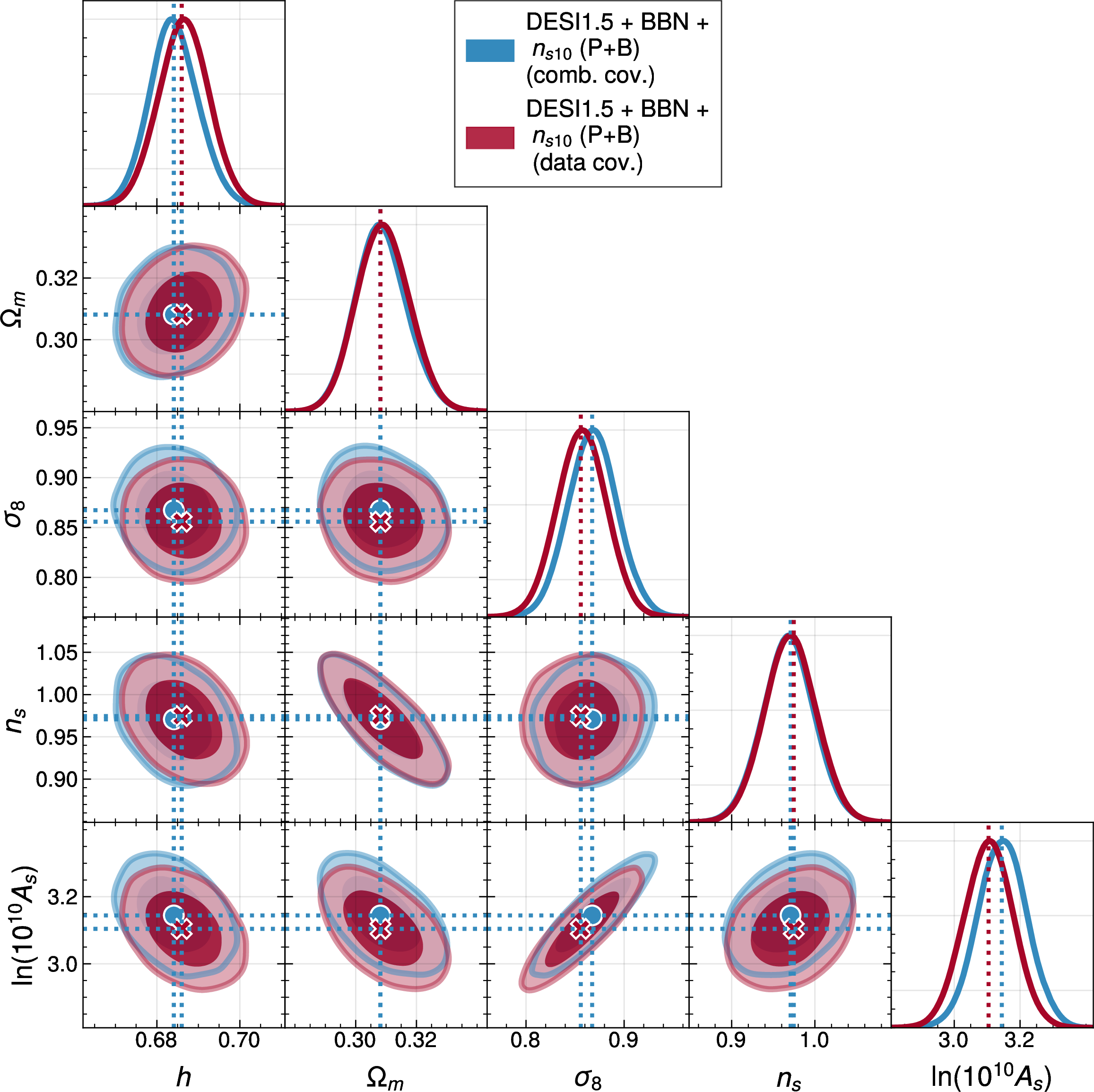
In [26] we found that in compressed variable space and for power spectrum information only, ignoring the covariance between DR1 FS and DR2 BAO does not affect cosmological inference in any significant way. For completeness, we repeat these tests while including the bispectra. 2 compares the \(\Lambda\)CDM constraints with and without the cross-covariance blocks \(\mathbf{r}^{\rm BAO\times SF}\). The absence of these blocks in the covariance results in a \(\sim 0.44\sigma\) shift in \(\sigma_8\) (\(0.55\sigma\) shift in \(\log(10^{10}A_s)\)) and a \(0.4\sigma\) shift in \(h\), but does not affect the overall constraining power. While the measurements are consistent within \(1\sigma\), such bias would likely induce biases in parameters that rely on the late-time clustering amplitude such as the neutrino masses. Consequently, we include the cross-covariance blocks for the rest of this work.

4.2 Cosmological inference↩︎
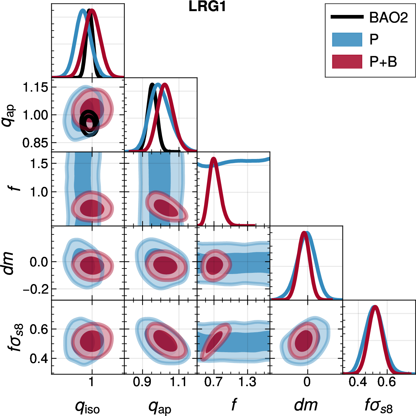
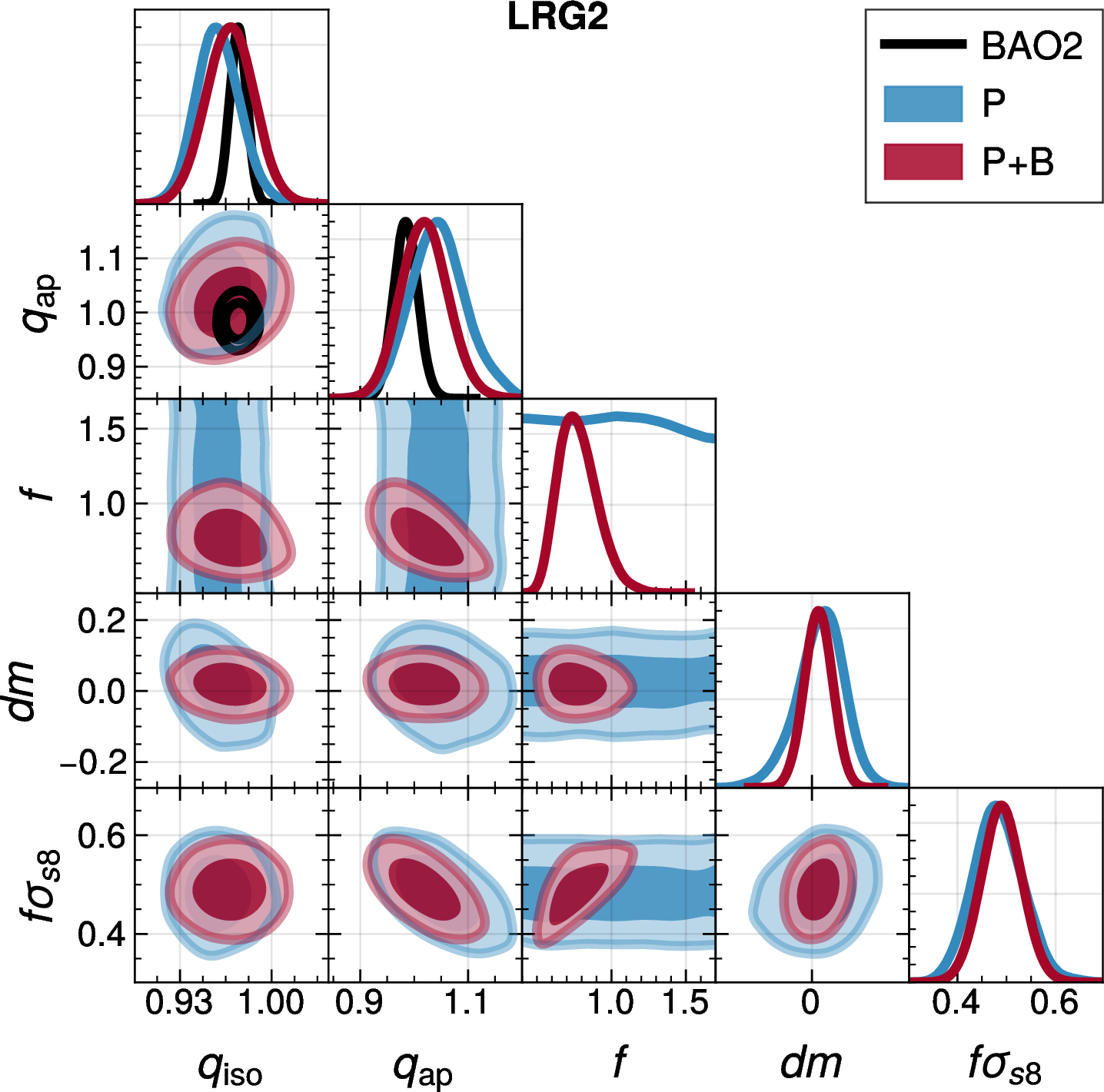
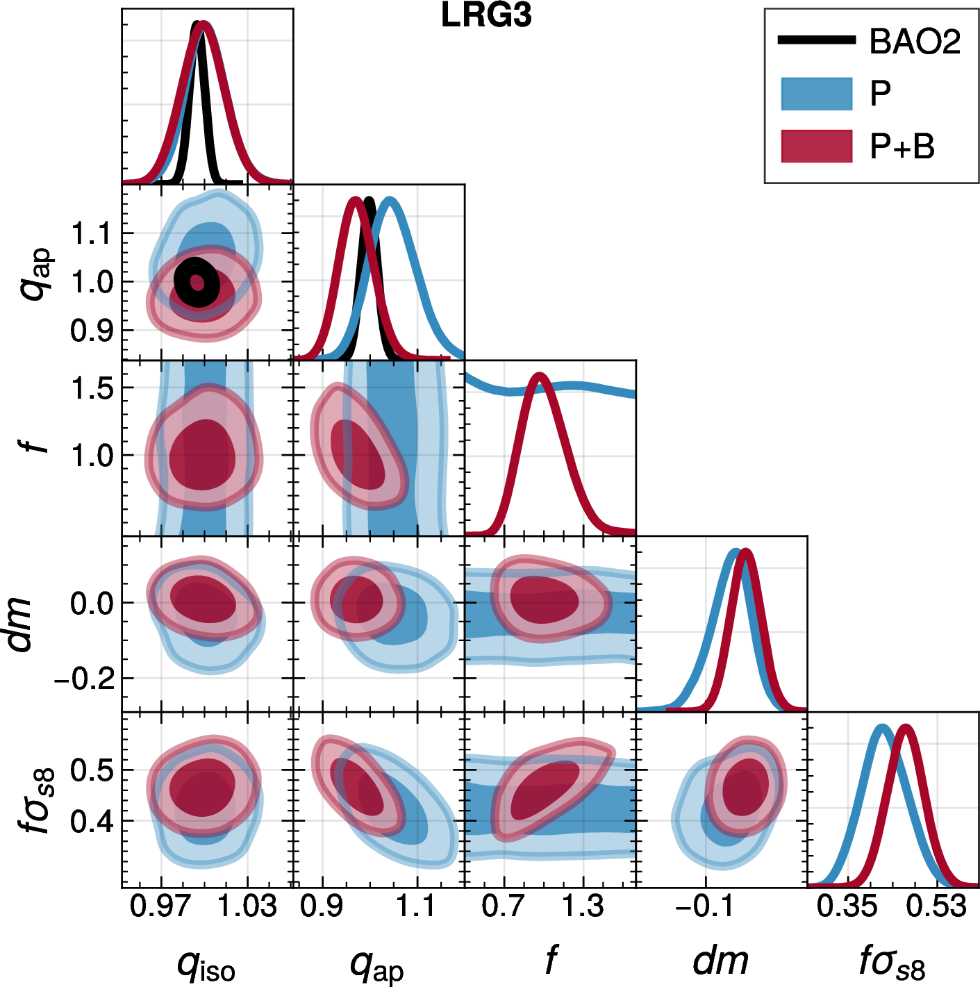
Figure 3: Comparison of 2-point (P) and 3-point (P+B)-based Shapefit constraints for the different DESI DR1 LRG bins. The 2-point measurements are those of Ref. [23] and the 3-point are from Ref. [28]. Since the power spectrum chains were run with a single degenerate parameter, we only show constraints for \(f\sigma_{s8}\) and a flat posterior for \(f\). On the other hand, for the bispectrum, both \(\sigma_{s8}\) and \(f\) are sampled independently thus we report both. We have added the contours for BAO2 as well for reference..
![Figure 4: Comparison of our results (DESI1.5 + Bispectrum, labeled P+B) to previous DESI1 and DESI1.5 analyses (using only the power spectrum, labeled “P”) in the context of \LambdaCDM. Constraints from DESI1 using FM from [24] shown for reference.](/article/2606.23936/plots/PvPB_lcdm_whisker.png "fig:")
| Dataset | \(h\) | \(\Omega_m\) | \(\sigma_8\) | \(n_s\) | \(S_8\) |
|---|---|---|---|---|---|
| DESI1.5 + BBN + \(n_{s10}\) (P+B) | \(0.6841 \pm 0.0059\) | \(0.3085 \pm 0.0085\) | \(0.868 \pm 0.025\) | \(0.969 \pm 0.031\) | \(0.880 \pm 0.026\) |
| DESI1.5 + BBN + \(n_{s10}\) (P) | \(0.6876 \pm 0.0059\) | \(0.3035 \pm 0.0085\) | \(0.822 \pm 0.034\) | \(0.965 \pm 0.032\) | \(0.827 \pm 0.036\) |
We first show the SF constraints for both power spectrum [23] and bispectrum [28] in 3. The plot shows that in the case of the bispectrum, we are able to independently constrain \(f\) and \(\sigma_{s8}\), while the power spectrum chains are run only using a single degenerate parameter \(f\sigma_{s8}\). No power spectrum chains were run sampling growth and amplitude independently since the 2-point clustering can’t disentangle this degeneracy so we show a band for \(f\) in this case. In addition we show the BAO constraints from [20] to show they are consistent with both P and P+B geometry constraints. We expect some differences between the P and P+B \(q_{\rm ap}\) parameter as the P+B results shown also include the hexadecapole of the power spectrum. Nonetheless, given that the BAO2 geometry constraints are much tighter, these will dominate when combining with the SF constraints to obtain cosmological parameter estimates.
While the addition of the bispectrum breaks the \(f-\sigma_{s8}\) degeneracy, in \(\Lambda\)CDM \(f\) is determined by \(\Omega_m\). Hence in this case the bispectrum is only expected to improve constraints on \(\sigma_8\).
4.2.1 \(\Lambda\)CDM constraints↩︎
Our baseline results are obtained including the minimum external data possible, i.e. BBN (\(\omega_b\)) and wide \(n_{s}\) priors as described in 2.3. 4 shows the \(\Lambda\)CDM constraints (also summarized in 2) obtained from the joint analysis (bottom line) as well as our previous DESI1.5 measurements in the middle row and the official DESI analysis in the top row.
\[\label{eq:lcdm95constraints} \begin{rcases} \Omega_m &= 0.3085 \pm 0.0085 \\ \sigma_8 &= 0.868 \pm 0.025 \\ h &= 0.6841 \pm 0.0059 \\ S_8 &= 0.880 \pm 0.026 \\ \end{rcases} \quad \text{DESI1.5 + BBN + n_{s10} (P+B)}\tag{5}\]
5 shows the final constraints obtained when including the LRG bispectrum. Compared to the previous analyses using only the power spectrum, adding the bispectrum shifts the inferred value of \(\sigma_8\) upward by \(1.1\sigma\) and \(S_8\) by \(1.2\sigma\) (compared to DESI1.5). Similarly high values of \(\sigma_8\) have also been reported from DESI data within the frequentist analysis of DR1 FS [62].
Furthermore, the constraints on these amplitude parameters improve considerably. The \(1\sigma\) uncertainty on \(\sigma_8\) shrinks by \(26.5\%\), while the error on \(S_8\) is reduced by \(27.8\%\). These improvements are consistent with the findings of [37] using only DR1 data, where the constraint on amplitude parameter \(\log(10^{10}A_s)\) also improved by roughly \(20\%\) due to the addition of the bispectra. These larger \(S_8\) values are in a \(\sim3\sigma\) tension with the DES Y6 results [63], [64] but are consistent (\(\sim1\sigma\)) with the CMB-only constraints [65], [66].
In contrast, the background parameters \(h\), \(\Omega_m\) and the spectral index \(n_s\) show only marginal shifts (less than \(2\%\)) and no significant change in their uncertainties as these are dominated by the BAO2 information already present in the DESI1.5 (P) analysis.
4.2.2 \(w_0w_a\)CDM Dynamical Dark Energy↩︎
| Dataset | \(h\) | \(\Omega_m\) | \(\sigma_8\) | \(n_s\) | \(w_0\) | \(w_a\) |
|---|---|---|---|---|---|---|
| DESI1.5 + BBN + \(n_{s10}\) (P) | \(0.645 \pm 0.022\) | \(0.351 \pm 0.025\) | \(0.782 \pm 0.038\) | \(0.956 \pm 0.039\) | \(-0.49 \pm 0.25\) | \(-1.52 \pm 0.77\) |
| DESI1.5 + BBN + \(n_{s10}\) (P+B) | \(0.651 \pm 0.022\) | \(0.342 \pm 0.026\) | \(0.838 \pm 0.032\) | \(0.972 \pm 0.040\) | \(-0.64 \pm 0.25\) | \(-1.04 \pm 0.80\) |
| DESI1.5 + CMB (P) | \(0.634 \pm 0.017\) | \(0.356 \pm 0.020\) | \(0.778 \pm 0.015\) | \(0.9667 \pm 0.0035\) | \(-0.38 \pm 0.20\) | \(-1.82_{-0.53}^{+0.66}\) |
| DESI1.5 + CMB (P+B) | \(0.640 \pm 0.017\) | \(0.351 \pm 0.019\) | \(0.789 \pm 0.015\) | \(0.9655 \pm 0.0036\) | \(-0.48 \pm 0.19\) | \(-1.57 \pm 0.55\) |
| DESI1.5 + BBN + \(n_{s10}\) + DES-Dovekie (P+B) | \(0.673 \pm 0.010\) | \(0.3168 \pm 0.0090\) | \(0.859 \pm 0.025\) | \(0.977 \pm 0.040\) | \(-0.882 \pm 0.064\) | \(-0.34 \pm 0.30\) |
| DESI1.5 + DES-Dovekie + CMB (P+B) | \(0.6723 \pm 0.0054\) | \(0.3160 \pm 0.0053\) | \(0.8147 \pm 0.0077\) | \(0.9669 \pm 0.0037\) | \(-0.817 \pm 0.055\) | \(-0.68 \pm 0.21\) |
When assuming a model with dynamical dark energy, we use the CPL [67], [68] parametrization. Our previous work provided the first robust Bayesian DESI-only constraints on this model using the FS data. In this work we further build on those by adding the bispectrum of the LRG, while still considering both the cross correlation between power spectra and bispectra as well as the cross correlation between BAO2 and FS data using the ShapeFit approach.
[tab:cosmo95params95w0wa] summarizes these constraints alongside a comparison with the previous DESI1.5 analyses. Similarly to the \(\Lambda\)CDM case, the additional three-point information yields \(1.2\sigma\) shift in the \(\sigma_8\) posterior mean, accompanied by a 18% reduction in uncertainty relative to the power-spectrum-only constraints. The dark energy equation-of-state parameters consistently migrate by \(\sim0.4\sigma\) toward the \(\Lambda\)CDM point.
6 shows our baseline constraints on DE where the constraint on each parameter are marginalized over all other parameters:
\[\label{eq:w0wacdm95constraints} \begin{rcases} w_0 &= -0.64 \pm 0.25 \\ w_a &= -1.04 \pm 0.80 \\ \end{rcases} \quad \text{DESI1.5 + BBN + n_{s10} (P+B)}.\tag{6}\]
A closer examination of the \(w_0\)–\(w_a\) plane (displayed in the top-left panel of 5) reveals that the inclusion of bispectrum information systematically shifts the joint confidence contours toward the \(\Lambda\)CDM point (\(w_0=-1\), \(w_a=0\)) along the degeneracy direction. In the two-dimensional plane, the \(\Lambda\)CDM point lies inside the \(1\sigma\) contour after adding the bispectrum, indicating consistency at that level. This might appear counterintuitive because the one-dimensional marginalised constraints reported in 6 exclude the \(\Lambda\)CDM values by more than \(1\sigma\) (e.g., \(w_0 = -0.64\pm0.25\) is \(1.4\sigma\) away from \(-1\)). The resolution of this apparent contradiction lies in the strong negative correlation between \(w_0\) and \(w_a\) inherent to the CPL parametrisation. The one-dimensional posteriors project the correlated two-dimensional contour onto each axis, thereby amplifying the deviation from \(\Lambda\)CDM in the marginalised distributions even when the joint posterior comfortably contains the \(\Lambda\)CDM point.
To underscore the robustness of this inference against prior-induced projection effects, we overlay the maximum a-posteriori (MAP) estimates for each analysis variant. This diagnostic helps distinguish genuine shifts in the likelihood peak from artifacts arising from marginalization over poorly constrained nuisance directions, which is a known concern in high-dimensional Bayesian analyses, where residual volume effects can displace contours along degeneracy trajectories even when alternative mitigation strategies are employed. We have also added the BAO2 contours to highlight the wealth of information present in the FS analysis.
These represent the most up-to-date and stringent DESI-only constraints (supplemented only by minimal external priors) on dynamical dark energy to date, showing no statistically significant preference for time-evolving dark energy.
In the top right panel of 5, we display the corresponding constraints when CMB data are incorporated: \[\begin{rcases} w_0 &= -0.48 \pm 0.19 \\ w_a &= -1.57 \pm 0.55 \\ \end{rcases} \quad \text{DESI1.5 + CMB (P+B)}.\] A comparable trend is observed: the addition of bispectrum information pulls the joint posterior toward \(\Lambda\)CDM, consistent with findings from the DR1-only analysis [37]. However, the inclusion of DR2 BAO measurements substantially tightens the credible regions, and the resulting CMB+DESI combination exhibits a \(2.8\sigma\)7 tension with \(\Lambda\)CDM—highlighting the enhanced constraining power of the expanded dataset while underscoring the persistent, albeit reduced, preference for dynamical dark energy in the joint CMB+ DESI analysis. We compute the Deviance Information Criterion (DIC)8 change between models to be \(\Delta \rm DIC \approx -7.8\), which indicates a strong preference (i.e. \(-10 < \Delta \rm DIC < -5\)) [69] for \(w_0w_a\)CDM even when somewhat accounting for the extra freedom penalty.
In addition to these, we also report constraints including SNe information (which can also be seen in the bottom panels of 5).
For the SNe + DESI1.5 alone we find \[\begin{rcases} w_0 &= -0.882 \pm 0.064 \\ w_a &= -0.34 \pm 0.30 \\ \end{rcases} \quad \text{DESI1.5 + BBN + n_{s10} + DES-Dovekie (P+B)}.\] These constraints are only \(1.57\sigma\) away from \(\Lambda\)CDM. This corresponds to a \(\Delta{\rm DIC}\approx -0.7\) which indicates no preference for evolving DE from DESI and SNe. On the other hand, adding back the CMB information, pulls the contours away to \(3.05\sigma\) or a \(\Delta {\rm DIC} \approx -9.1\) which does suggest a strong preference for \(w_0w_a\)CDM from this combination, implying that it is mostly the CMB information which drives the constraints away from \(\Lambda\)CDM. \[\begin{rcases} w_0 &= -0.817 \pm 0.055 \\ w_a &= -0.68 \pm 0.21 \\ \end{rcases} \quad \text{DESI1.5 + CMB + DES-Dovekie (P+B)}\]
A direct comparison with the Bayesian evidence analysis of [70] reveals differences in the inferred model preference. While our DIC‑based results suggest a \(2.8\sigma\) preference for \(w_0w_a\)CDM when CMB is added, Ref. [70] find that for a similar combination (BAO2 + CMB [Camspec] + DES‑Dovekie) the full evidence favors \(\Lambda\)CDM (\(\log B = -0.01\pm0.27\)). Additionally, their results in the BAO2 + CMB combination shows the evidence for \(w_0w_a\)CDM is weak at best regardless of the CMB likelihood chosen. They report a \(\log B\approx 0.5\) (i.e. \(1.5\sigma\) Bayesian significance) for Planck PR3 and \(\log B\approx -0.6\) for Camspec (preference for \(\Lambda\)CDM). This indicates that the approximate DIC penalty may be insufficient to fully account for the additional parameters of the \(w_0w_a\)CDM, leading to an overstatement of the preference compared to the exact Bayesian evidence. Notably, the inclusion of the LRG bispectrum systematically shifts our dark energy constraints toward \(\Lambda\)CDM (see [tbl:tab:cosmo95params95w0wa] and 5), a trend consistent with independent supernova reanalyses [22]. The bispectrum thus further mitigates this preference by breaking degeneracies that previously allowed the data to favor a more complex dark energy sector.
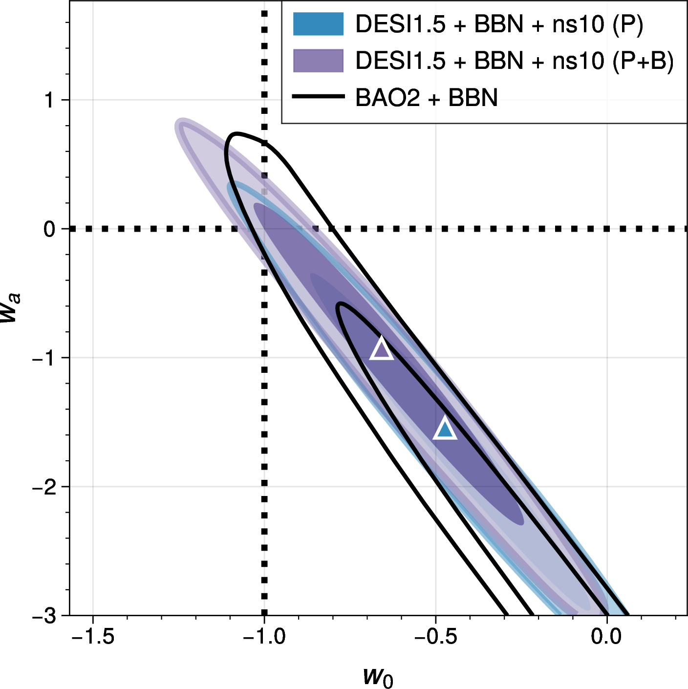
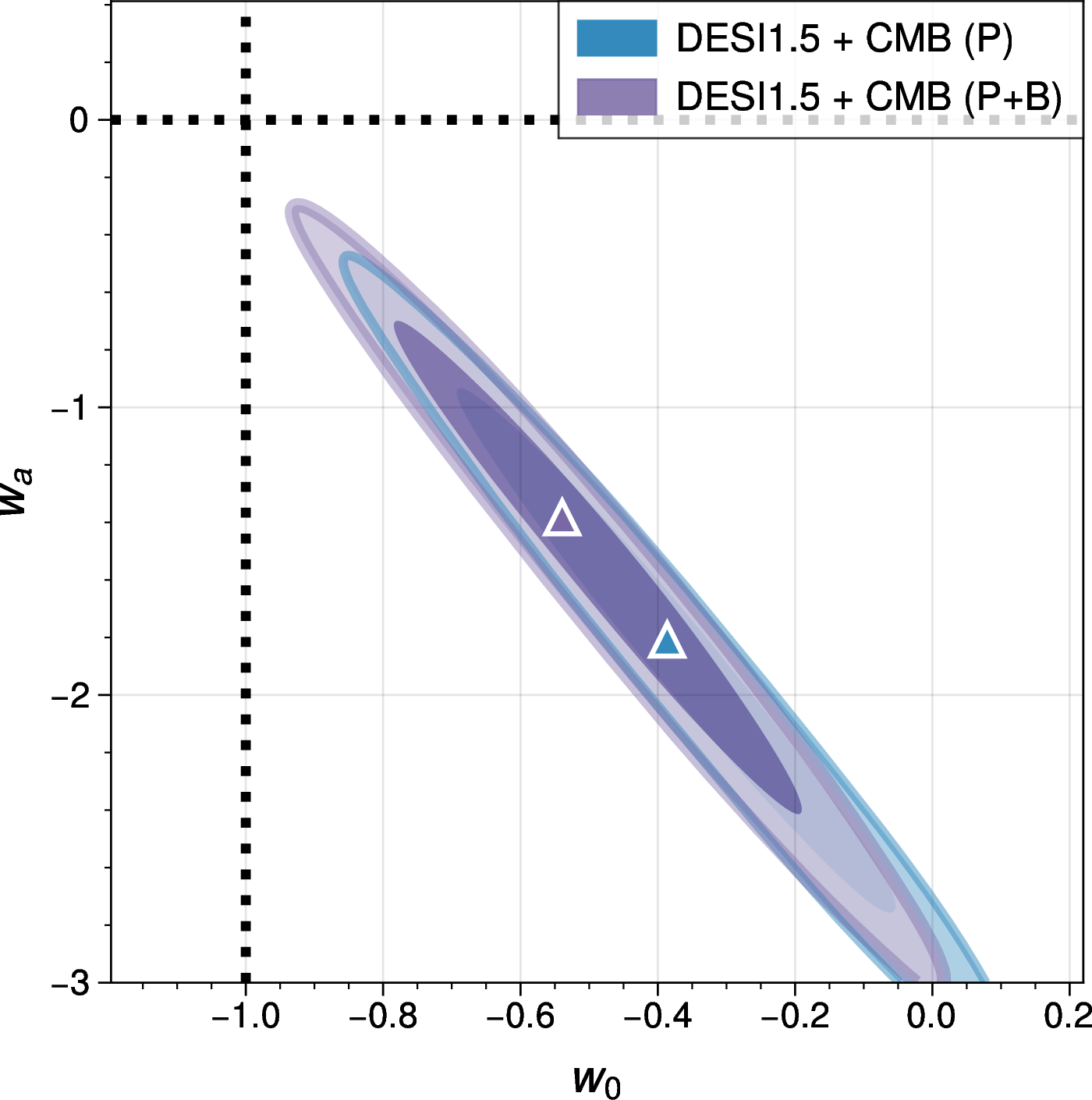
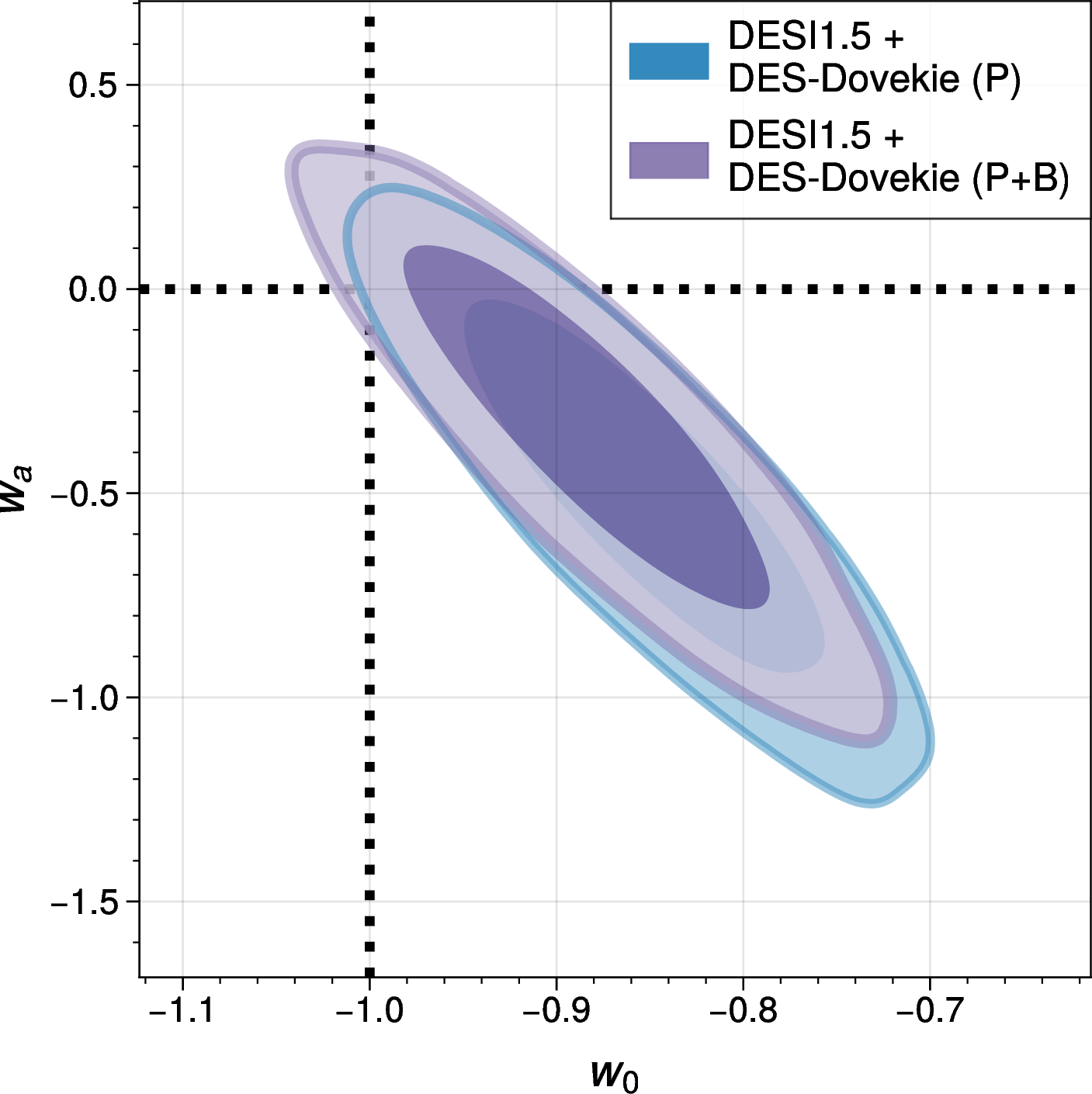
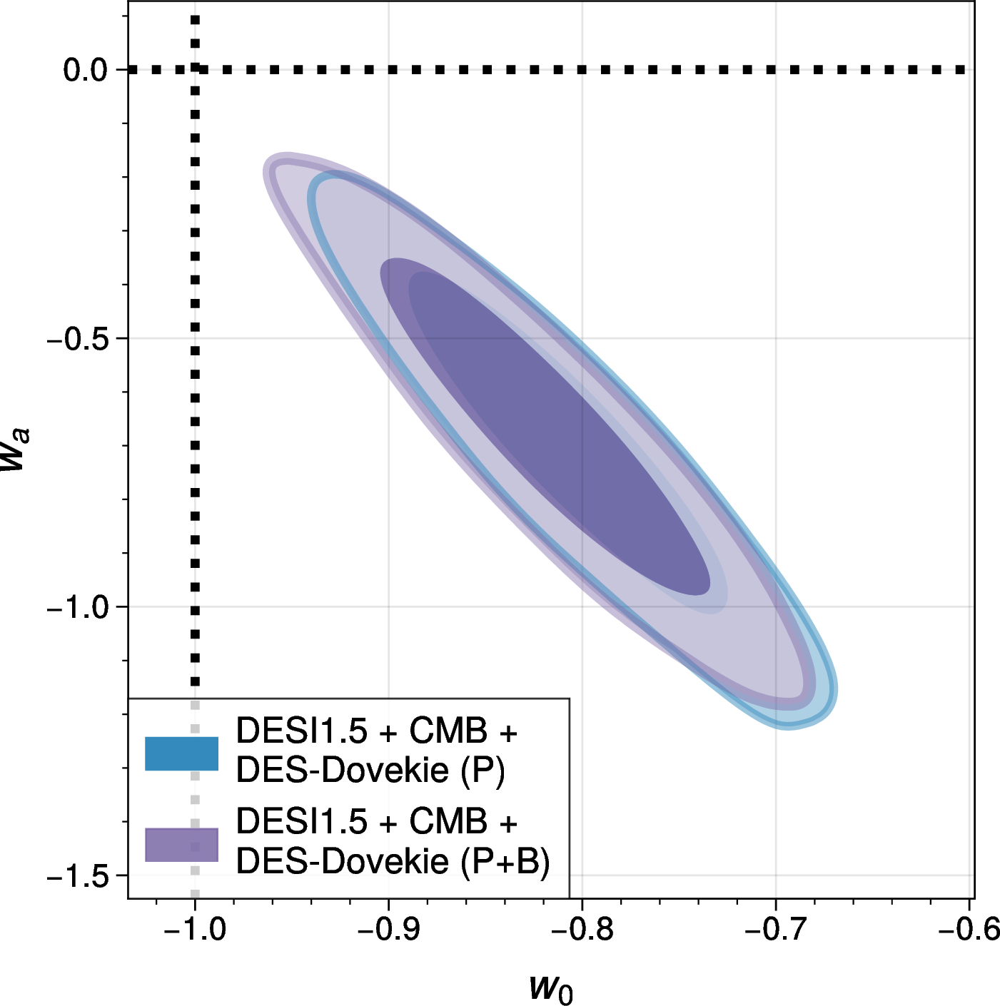
Figure 5: Dark energy equation-of-state constraints from DESI1.5 with and without the addition of the LRG bispectra. Top left: Parameter constraints with minimal external data. We have added the MAP points for the FS constraints to highlight the absence of projection effects, as well as the BAO2 constraint to highlight the information content of FS analyses. Top right: DE constraints adding CMB. Bottom left: Constraints only with SNe from DES. Bottom right: DE constraints combining all datasets..
4.2.3 Neutrino mass constraints↩︎
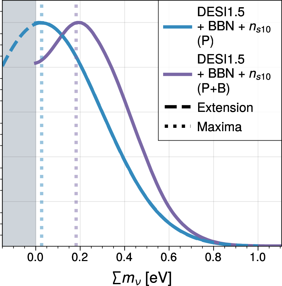
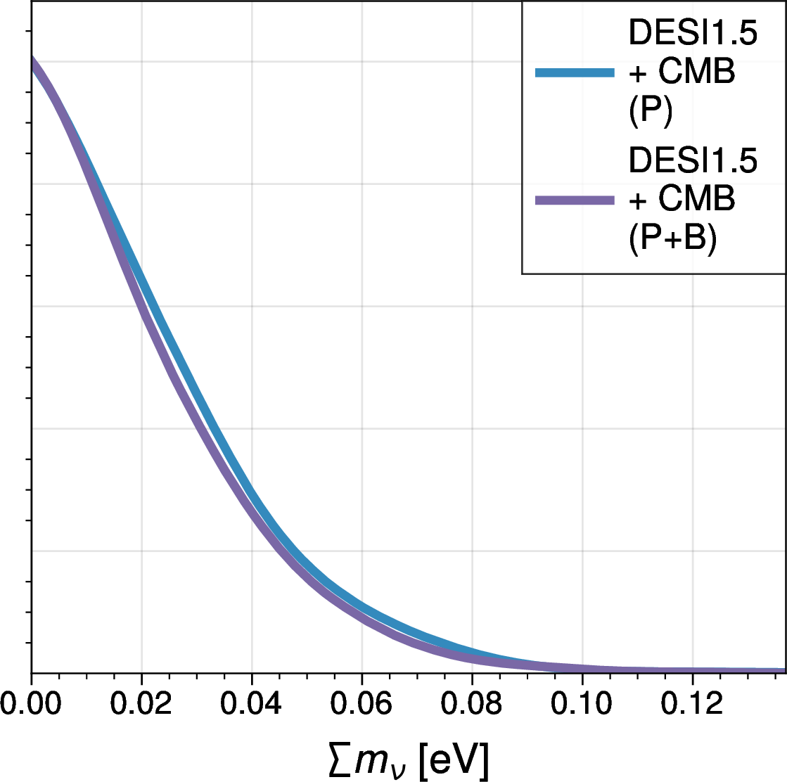
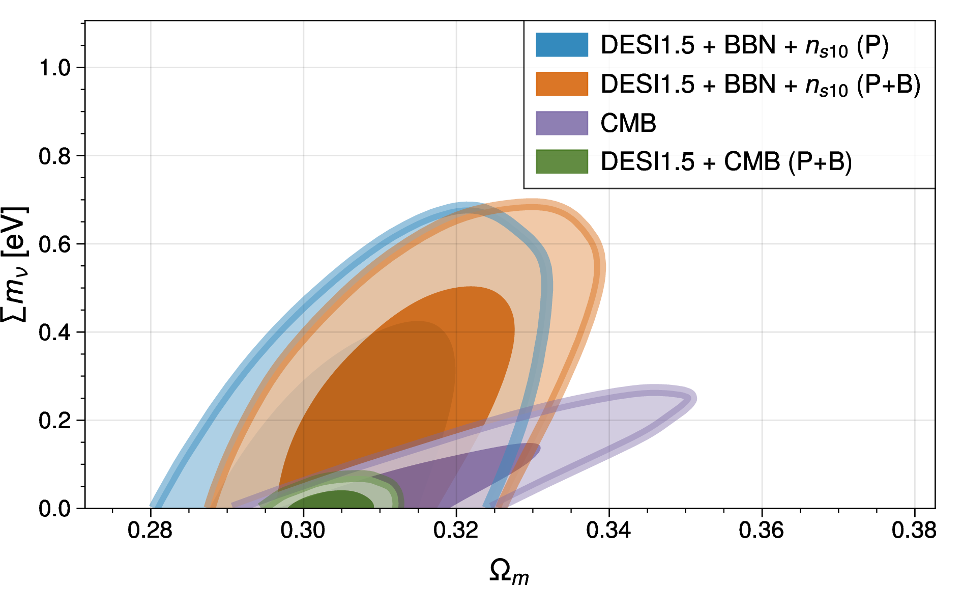
Figure 6: Neutrino mass constraints from the DESI1.5 dataset including the LRG bispectra compared to previous analyses without it. Top left: Constraints from DESI with minimal priors. Dashed lines show the extended Gaussian profile and dotted lines show the approximate MAP points. Top right: Constraints including CMB [Camspec]. Bottom: \(\sum m_{\nu}\)—\(\Omega_m\) plane showing the degeneracy breaking between CMB and DESI1.5..
The bispectrum is also sensitive to the late-time suppression from neutrino free-streaming and is thus an important observable for neutrino physics [71]–[75]. Our DESI‑only constraints (with BBN and \(n_{s10}\) priors) illustrate this sensitivity. The power‑spectrum–only analysis (P) yields a marginalized mean of \(\sum m_\nu = 0.23^{+0.059}_{-0.225}~\rm eV\), which is consistent with zero and has a long tail towards high masses. The addition of BAO2 to DR1 FS in [26] moved the MAP towards slightly positive values, similarly, adding the bispectrum shifts the mean and 95% CL to \[\begin{rcases} \sum m_{\nu} = 0.26\pm0.17~\rm eV\quad\text{68\% CI}\\ \sum m_{\nu} < 0.5698~\rm eV\quad\text{95\% CL} \end{rcases} \quad \text{DESI1.5 + BBN + n_{s10} (P+B), \LambdaCDM{}} ,\] further moving the posterior peak into the positive region. Consequently, the 95% level also moves further away from zero. This can be observed in the top left panel of 6. These neutrino mass constraints are still consistent with our previous power-spectrum-only analyses [26] and with experiments such as KATRIN’s constraint of 9 \(\sum m_\nu \lesssim 0.93~\rm eV\) [76]. Moreover, the recovered peak in the positive mass range is in line with the lower mass bounds of \(\sum m_\nu \gtrsim 0.058~\rm eV\) for normal ordering and \(\sum m_\nu \gtrsim 0.98~\rm eV\) for inverted ordering provided in [77] from neutrino oscillations.
The addition of CMB [Camspec] (top right in 6) dominates the neutrino mass constraints and drives the peak back to the negative mass range regardless of the DESI1.5 data preference. The resulting constraints are tighter than without the bispectrum at \[\sum m_{\nu} < 0.0590~\rm eV\quad \text{95\% CL, DESI1.5 + CMB (P+B), \LambdaCDM{}}\] This constraint is still driven by the \(\sum m_\nu\)—\(\Omega_m\) degeneracy breaking between DESI and CMB data as illustrated in the bottom panel of 6. These tight constraints seem in tension with the lower bounds from neutrino oscillations [77], but are quite sensitive to the CMB likelihood used. One might speculate that perhaps alternative CMB likelihoods, such as those which mitigate the lensing anomaly, may alleviate this tension.
4.2.4 \(\nu w_0w_a\)CDM constraints↩︎
When including evolving DE along with neutrinos we find the same trend in DE behavior, the bispectrum tends to shift contours towards the non-evolving limit of \(\Lambda\)CDM (See 7), albeit with increased uncertainties due to the additional degree of freedom in the neutrino mass sum. The neutrino masses in turn also show a shift towards the positive mass end and we can therefore quote a constraint \[\begin{rcases} \sum m_{\nu} &= 0.49 \pm 0.31~\mathrm{eV}\quad\text{68\% CI}\\ \sum m_{\nu} &< 1.046~\mathrm{eV}\quad \text{95\% CL} \\ w_0 &= -0.56 \pm 0.25 \\ w_a &= -1.54_{-1.21}^{+0.61} \\ \end{rcases} \quad \text{DESI1.5 + BBN + n_{s10} (P+B)}.\]
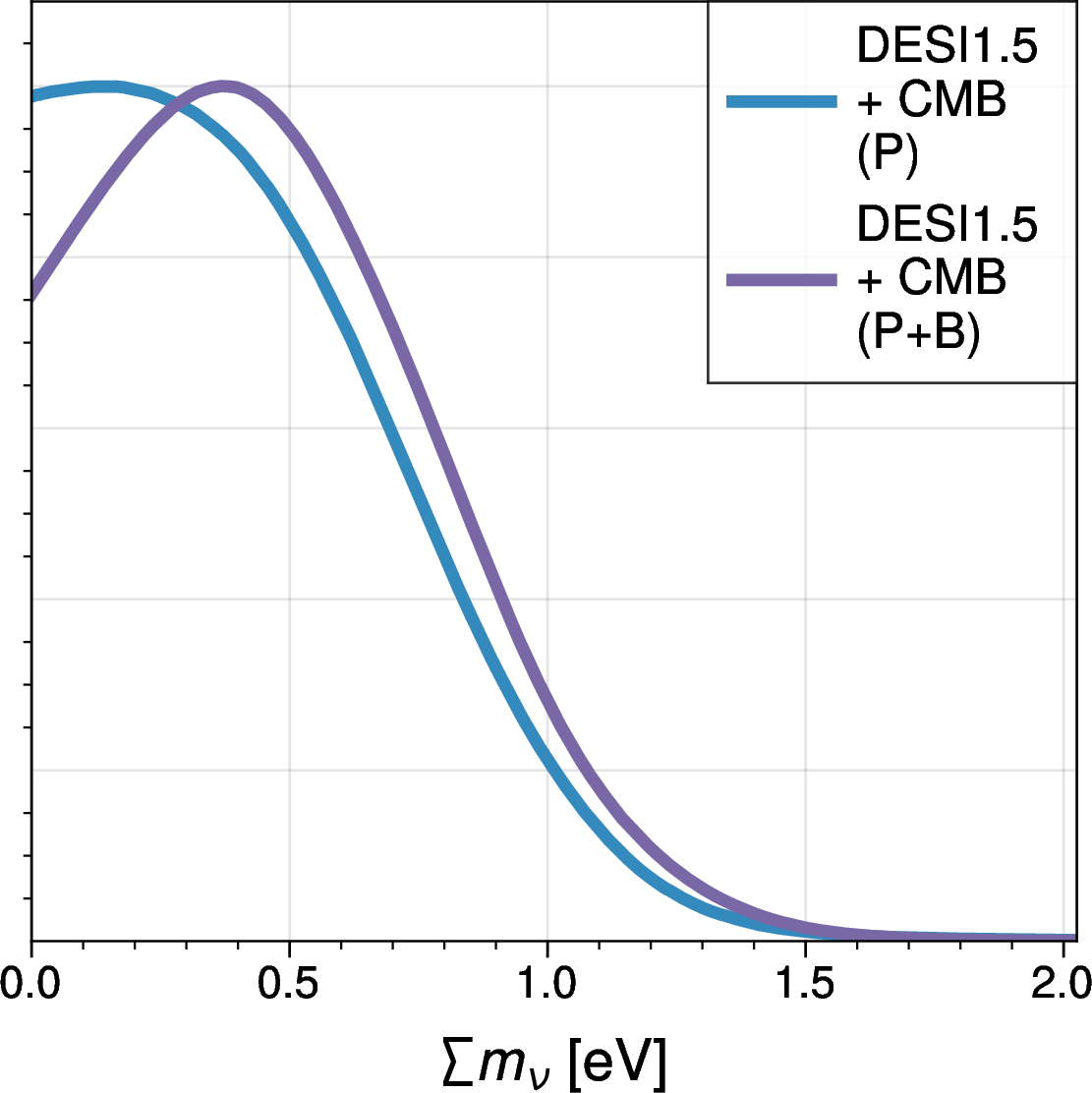

Figure 7: Cosmological constraints on a \(\nu w_0w_a\)CDM model with and without bispectra. Left: Marginalized posteriors on the sum of neutrino masses, notice the shift towards positive values. Right: Constraints on DE parametrization showing the shift towards \(\Lambda\)CDM induced by the addition of the bispectra..
These are once again fully consistent with the expectations from neutrino oscillation experiments both in the upper and lower bounds.
4.2.5 Constraints on spatial curvature↩︎
Finally, we can explore the effect of the bispectrum information on the inferred constraints on the spatial curvature.
8 shows the curvature constraints from DESI1.5 without CMB (left panel) and with CMB [Camspec] (right), plotted against the physical matter density. In our DESI-only constraints, the addition of the bispectrum shifts the central value towards positive \(\Omega_k\) by \(0.6\sigma\) without altering significantly the size of the error uncertainties.
| Dataset | \(\Omega_k\) | \(h\) | \(\Omega_m\) | \(\sigma_8\) | \(n_s\) | |
|---|---|---|---|---|---|---|
| DESI1.5 + BBN + \(n_{s10}\) (P) | \(0.007 \pm 0.024\) | \(0.685 \pm 0.011\) | \(0.3042 \pm 0.0090\) | \(0.826 \pm 0.037\) | \(0.970 \pm 0.039\) | |
| DESI1.5 + BBN + \(n_{s10}\) (P+B) | \(0.022 \pm 0.024\) | \(0.677 \pm 0.010\) | \(0.3078 \pm 0.0089\) | \(0.873 \pm 0.026\) | \(0.989 \pm 0.040\) | |
| DESI1.5 + CMB (P) | \(0.0028 \pm 0.0011\) | \(0.6857 \pm 0.0030\) | \(0.3035 \pm 0.0036\) | \(0.8154_{-0.0055}^{+0.0051}\) | \(0.9639 \pm 0.0037\) | |
| DESI1.5 + CMB (P+B) | \(0.0027 \pm 0.0011\) | \(0.6828 \pm 0.0031\) | \(0.3072 \pm 0.0034\) | \(0.8177 \pm 0.0055\) | \(0.9630 \pm 0.0040\) |
The shift toward positive \(\Omega_k\) suppresses the growth of structure, which would reduce the predicted clustering amplitude. However, the bispectrum forces a higher observed amplitude, and the fit compensates by raising \(\sigma_8\). The constraints on the full parameter space are shown in [tbl:tab:olcdm]. Indeed, the constraint on \(\sigma_8\) improves by \(14\%\) when the bispectrum is included. At the same time, \(h\) and \(\Omega_m\) shift by \(0.4\sigma\) and \(0.8\sigma\), respectively, relative to the earlier DESI1.5 combination. Crucially, the physical matter density \(\omega_m = h^2\Omega_m\) remains nearly unchanged (a \(0.2\sigma\) shift) and shows a modest \(4.3\%\) improvement in its uncertainty. A modest improvement in the physical matter density is expected from the additional information that the bispectrum brings on the the SF parameter \(m\) [27], [78], [79] whose bounds have been shown to be tightened when adding the bispectrum [28].
In a joint analysis with the CMB, the bispectrum does not affect the curvature constraints, and the inference still show a \(2\sigma\) preference for positive \(\Omega_k\). The constraint of the physical matter density however is improved by 7% .
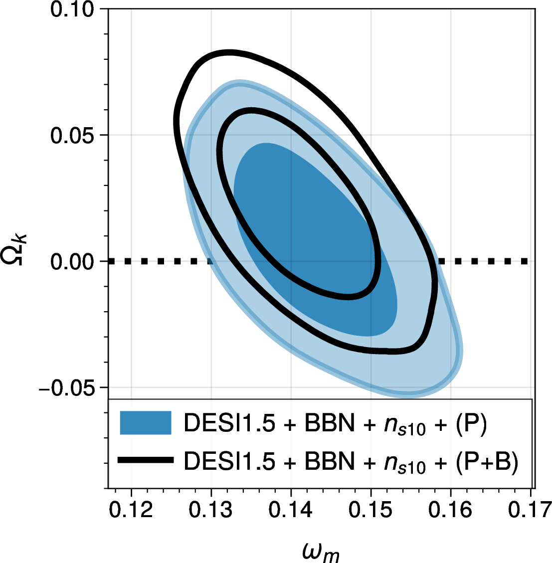
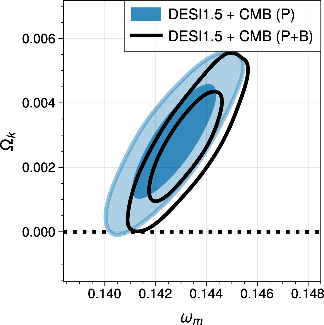
Figure 8: Constraints on the spatial curvature of the Universe from DESI1.5 with the bispectrum, compared to those without. Filled contours show results from [26] using only the power spectrum, line contours show results from this work using the LRG bispectra..
4.2.6 Modified gravity↩︎
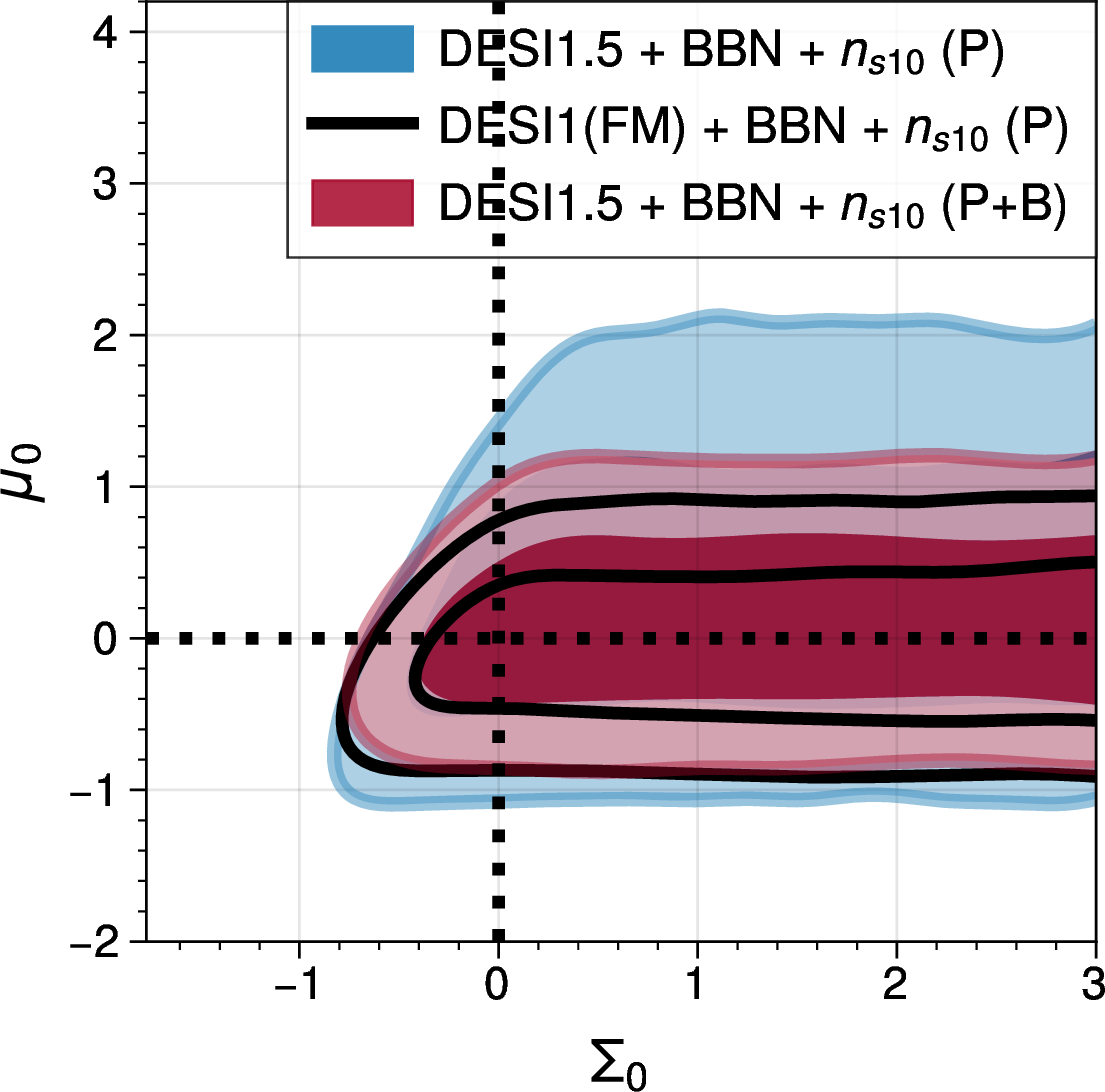
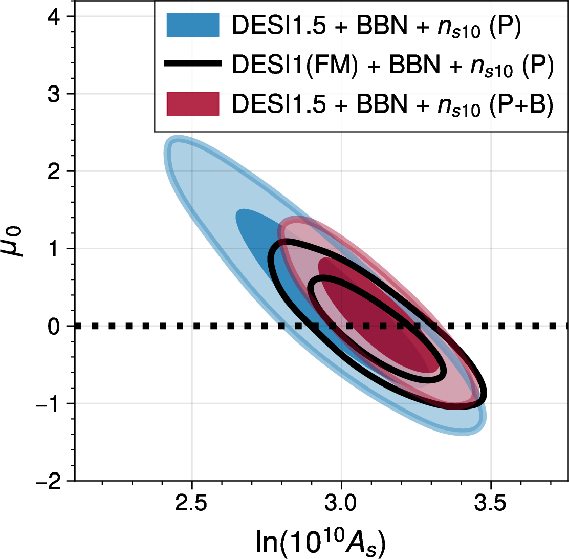
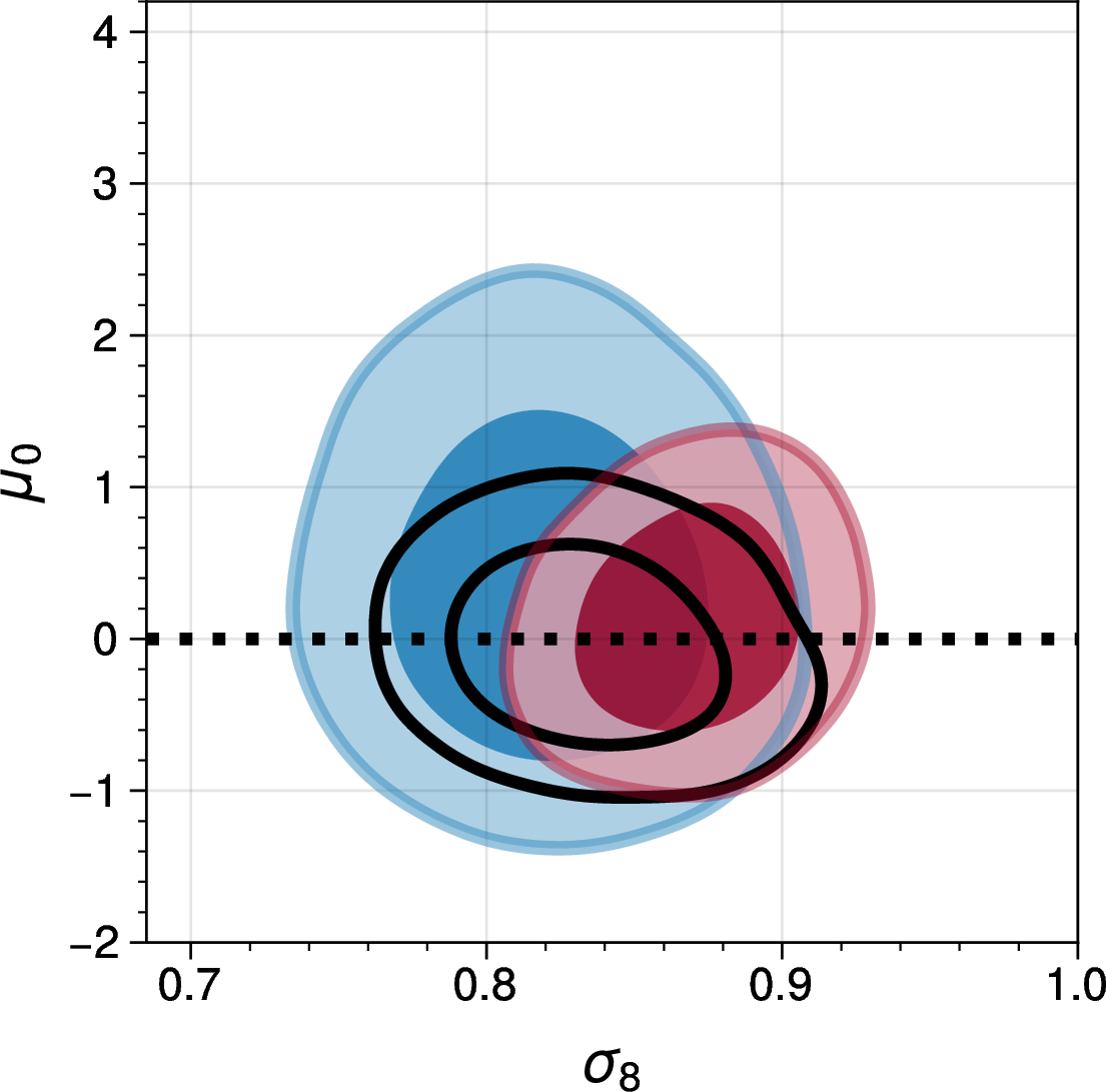
Figure 9: Modified gravity constraints from DESI1.5 and DESI1(FM) datasets for different parameter projections. Top left panel shows the MG parameter plane, showing an unconstrained \(\Sigma_0\). The top right panel shows the degeneracy between the primordial amplitude \(A_s\) and the \(\mu_0\) parameter. The bottom panel shows the constraints on the late time amplitude parameter \(\sigma_8\), which is fully unconstrained with SF unless the bispectrum information is included to break the growth-amplitude degeneracy. FM is able to break this degeneracy on its own due to \(f\) being derived from the cosmology instead of a parameter in the model. Breaking the growth-amplitude degeneracy allows us to recover amplitude constraints using SF..
| Dataset | \(h\) | \(\Omega_m\) | \(\sigma_8\) | \(n_s\) | \(\ln(10^{10}A_s)\) | \(\mu_0\) | \(\Sigma_0\) |
|---|---|---|---|---|---|---|---|
| DESI1.5 + BBN + \(n_{s10}\) (P) | \(0.6871 \pm 0.0061\) | \(0.3033 \pm 0.0088\) | \(0.821 \pm 0.035\) | \(0.965 \pm 0.032\) | \(2.96 \pm 0.22\) | \(0.36 \pm 0.77\) | Unc. |
| DESI1(FM) + BBN + \(n_{s10}\) (P) | \(0.6871 \pm 0.0077\) | \(0.2946 \pm 0.0097\) | \(0.835 \pm 0.031\) | \(0.995 \pm 0.027\) | \(3.11 \pm 0.15\) | \(-0.04 \pm 0.44\) | Unc. |
| DESI1.5 + BBN + \(n_{s10}\) (P+B) | \(0.6842 \pm 0.0060\) | \(0.3085 \pm 0.0084\) | \(0.869 \pm 0.025\) | \(0.967 \pm 0.031\) | \(3.12 \pm 0.13\) | \(0.12 \pm 0.49\) | Unc. |
The constraining power of the compressed SF approach in a modified gravity (MG) scenario is largely dependent on the parametrization. In this work we adopt the same \(\mu_0\)–\(\Sigma_0\) parametrization used by earlier DESI studies on the matter using the FM approach [24], [25]. This parametrization is a first-order approach to an effective modification of the gravity equations that relates the potentials \(\Psi\) and \(\Phi\) with the sources \(\rho_i\Delta_i\) as \[\begin{align} k^2\Psi &= -4\pi G a^2\mu(a,k)\sum\rho_i\Delta_i\\ k^2(\Phi + \Psi) &= -8\pi G a^2\Sigma(a,k)\sum\rho_i\Delta_i. \end{align}\] The functions \(\mu(a,k)\) and \(\Sigma(a,k)\) are equal to 1 in general relativity (GR) but deviate in MG scenarios. In our approach we ignore the scale dependence and parametrize them both as \[\begin{align} \mu(a,k) &= 1 + \mu_0\frac{\Omega_{\rm DE}}{\Omega_\Lambda}\\ \Sigma(a,k) &= 1 + \Sigma_0\frac{\Omega_{\rm DE}}{\Omega_\Lambda}, \end{align}\] and use \(\mu_0\) and \(\Sigma_0\) as our effective parameters. In GR these are both equal to 0. Given that we focus on DESI data only, the \(\Sigma_0\) parameter is unconstrained as it does not enter the geodesic equations of matter particles, and therefore it does not affect the clustering of matter, DESI however should be able to constrain \(\mu_0\) which modifies the growth of structure [80].
9 compares the 2D marginalized posteriors from DESI1.5 power‑spectrum–only (P), DESI1.5 with bispectrum (P+B), and the official DESI DR1 full‑modeling (FM) analysis [24]. As expected, \(\Sigma_0\) is completely unconstrained without lensing information (top‑left panel). Without the bispectrum, the ShapeFit (SF) approach only measures the degenerate combination \(f\sigma_8\) and therefore cannot independently constrain \(f\) and \(\sigma_8\); consequently, \(\sigma_8\) (bottom panel) and \(\log(10^{10}A_s)\) (top‑right panel) are better constrained in FM, which derives \(f\) directly from the underlying cosmology and thus decouples growth from amplitude parameters.
Adding the bispectrum in SF breaks the growth–amplitude degeneracy, allowing separate constraints on \(f\) and \(\sigma_8\), which improves the \(\mu_0\) constraints by \(\sim 50\%\). Nevertheless, our \(\mu_0\) constraint remains \(\sim10\%\) weaker than FM. This is likely because our bispectrum information is limited to the LRG samples, whereas FM uses the power‑spectrum shape of all tracers (including ELGs and QSOs) to constrain growth. In contrast, \(\sigma_8\) is \(\sim20\%\) tighter in our P+B analysis than in FM, and \(\log(10^{10}A_s)\) is \(\sim10\%\) tighter, in line with the observations in other cosmological models. The DR2 BAO data (which only affect background parameters) do not contribute to these amplitude improvements. Our full parameter constraints are summarized in [tbl:tab:mgcdm].
The bispectrum information is also able to tighten the constraints on \(\sigma_8\) relative to the FM analysis by about 20% while shifting the central value up by \(\sim1.4\sigma\). The constraints on \(h\) and \(\Omega_m\) are also improved due to the more constraining BAO2 information at a similar level than in the GR case. In terms of MG, we find \[\begin{rcases} \mu_0 &= 0.12 \pm 0.49 \\ \gamma &= 0.553 \pm 0.005 \end{rcases} \quad \text{DESI1.5 + BBN + n_{s10} (P+B),\;MG},\] where we have derived a growth index \(\gamma\) value using [81] \[\require{physics} \begin{align} \gamma(\mu)&\approx\frac{1}{2} + \frac{0.161}{1.967 + \beta(\mu)}\\ \beta(\mu)&\approx\frac{1}{4}\qty[\sqrt{1 + 24\mu} - 1]. \end{align}\] These constraints are consistent with GR.
5 Conclusions↩︎
We have presented cosmological constraints from the combination of DESI Data Release 1 (DR1) full‑shape (FS) measurements, including the LRG bispectrum, and DESI Data Release 2 (DR2) baryon acoustic oscillation (BAO) measurements. The joint analysis properly accounts for the cross‑covariance between the two datasets using mock‑based estimates. The full‑shape information is compressed via the ShapeFit methodology, which mitigates prior volume effects that have hampered previous beyond‑\(\Lambda\)CDM analyses. Crucially, by circumventing these projection effects, our analysis yields robust, DESI-only constraints in extended models. This allows us to rigorously assess DESI’s independent constraining power as a standalone probe.
In the flat \(\Lambda\)CDM model with minimal external priors (BBN and a loose \(n_s\) prior), the inclusion of the LRG bispectrum (P+B) shifts the clustering amplitude upward: \(\sigma_8\) increases by \(1.1\sigma\) (from \(0.822\pm0.034\) to \(0.868\pm0.025\)) and \(S_8\) by \(1.2\sigma\) (from \(0.827\pm0.036\) to \(0.880\pm0.026\)). The uncertainties on these amplitude parameters improve by \(26\%\) and \(28\%\), respectively, demonstrating the bispectrum’s ability to break the degeneracy between galaxy bias and the underlying matter fluctuation amplitude. Background parameters (\(h\), \(\Omega_m\), \(n_s\)) show only marginal shifts, as their precision is dominated by the BAO data.
In the \(w_0w_a\)CDM model with DESI‑only data, the bispectrum shifts the dark energy equation‑of‑state parameters toward the \(\Lambda\)CDM point: \(w_0\) moves from \(-0.49\pm0.25\) to \(-0.64\pm0.25\) and \(w_a\) from \(-1.52\pm0.77\) to \(-1.04\pm0.80\) (each shift \(\sim0.4\sigma\)). The resulting DESI1.5 constraints in the \(w_0\)–\(w_a\) plane show no statistically significant preference for deviations from a cosmological constant. When CMB data are included, the DESI+CMB (P+B) combination exhibits a \(2.8\sigma\) (frequentist) preference for evolving dark energy, which decreases to \(1.6\sigma\) for DESI+DES‑Dovekie and rises to \(3.1\sigma\) for the full combination. We perform additional approximate DIC tests to take into account model complexity in our comparison and find that whenever CMB is included, the data prefers evolving DE, while combinations without CMB show no strong preference. This points towards the extra flexibility accommodating existing tensions between the datasets, such as the \(\Omega_m\) tension between DESI and CMB. Furthermore, a comparison with full Bayesian evidence analyses on similar data combinations [70] indicates that these \(\Delta\chi^2\)-derived significances may overstate the preference because the DIC penalty approximates model complexity less severely than the exact Ockham factor. The addition of the bispectrum consistently shifts the posteriors toward \(\Lambda\)CDM, weakening the evidence for time‑varying dark energy relative to power‑spectrum–only analyses.
The bispectrum provides enhanced sensitivity to the suppression of structure growth by massive neutrinos. In the DESI‑only analysis (BBN\(+n_{s10}\)), the power‑spectrum–only posterior for \(\sum m_\nu\) is consistent with zero, whereas adding the bispectrum yields a mean of \(0.26\pm0.17~\)eV and a \(95\%\) upper limit of \(0.57~\)eV, shifting the peak into the positive region and placing it in agreement with upper and lower bounds set by oscillation experiments. When CMB data are added, the constraint tightens dramatically (\(\sum m_\nu<0.059~\)eV at \(95\%\) CL), driven by the strong complementarity between DESI and CMB. Even when the background is relaxed to include evolving dark energy, DESI alone constraints neutrino masses to \(\sum m_\nu = 0.49\pm0.31~\)eV, again consistent with oscillation bounds.
In terms of spatial curvature, in DESI‑only analyses the bispectrum shifts the mean of \(\Omega_k\) from \(0.007\pm0.024\) to \(0.022\pm0.024\), a \(0.6\sigma\) shift, without improving the uncertainty. The physical matter density \(\Omega_m h^2\) remains stable and slightly better constrained (\(4.3\%\) improvement), as expected from the additional information the bispectrum brings to the ShapeFit parameter \(m\). When CMB data are included, the constraints on curvature remain consistent with previous power-spectrum-only analyses and show a \(\sim2\sigma\) preference for a positive \(\Omega_k\).
In the modified gravity sector, the ShapeFit compression without the bispectrum cannot independently constrain \(f\) and \(\sigma_8\) because it only measures the degenerate combination \(f\sigma_8\). Adding the LRG bispectrum (partially) breaks this degeneracy, improving the \(\mu_0\) constraint by \(\sim50\%\) and yielding \(\mu_0 = 0.12\pm0.49\) (\(68\%\) CI) from DESI‑only data which is fully consistent with general relativity (GR). Compared to full modeling (FM), our \(\mu_0\) constraint remains \(\sim10\%\) weaker, likely because FM uses the power‑spectrum shape of all tracers (including ELGs and QSOs) to constrain growth (i.e. \(f\)), whereas our bispectrum information is limited to LRG samples. Nevertheless, our P+B analysis tightens \(\sigma_8\) by \(\sim20\%\) and \(\log(10^{10}A_s)\) by \(\sim10\%\) relative to FM, in line with improvements seen in other cosmological models. Furthermore, we obtain an approximate \(\gamma = 0.553 \pm 0.005\) which is also consistent with the GR value. The inclusion of the LRG bispectrum thus provides a robust handle on modified gravity from DESI alone, even with a compressed approach.
Our analysis builds on our previous work [26], [28], [37] and demonstrates the power of combining the DR1 bispectrum with DR2 BAO while correctly accounting for their correlation. The ShapeFit compression allows robust Bayesian inference in extended models without the prior volume effects that affect full modeling approaches. The inclusion of the LRG bispectrum consistently shifts amplitude parameters upward, tightens their uncertainties, moves dark energy posteriors toward \(\Lambda\)CDM and provides a handle on modified gravity from DESI alone with a compressed approach.
Data availability↩︎
The data to reproduce the figures in this paper is available in the DESI zenodo repository https://doi.org/10.5281/zenodo.20592803. (Public after acceptance)
Acknowledgements↩︎
DFS and HGM acknowledge support through the Consolidación Investigadora (CNS2023-144605) of the Spanish Ministry of Science and Innovation. HGM also acknowledges the support of the Ramón y Cajal (RYC-2021-034104). Funding for this work was partially provided by the Spanish MINECO under project PID2022-141125NB-I00 MCIN/AEI, and the “Center of Excellence Maria de Maeztu 2020- 2023” award to the ICCUB (CEX2019-000918-M funded by MCIN/AEI/10.13039/501100011033).
This material is based upon work supported by the U.S. Department of Energy (DOE), Office of Science, Office of High-Energy Physics, under Contract No. DE–AC02–05CH11231, and by the National Energy Research Scientific Computing Center, a DOE Office of Science User Facility under the same contract. Additional support for DESI was provided by the U.S. National Science Foundation (NSF), Division of Astronomical Sciences under Contract No. AST-0950945 to the NSF’s National Optical-Infrared Astronomy Research Laboratory; the Science and Technology Facilities Council of the United Kingdom; the Gordon and Betty Moore Foundation; the Heising-Simons Foundation; the French Alternative Energies and Atomic Energy Commission (CEA); the National Council of Humanities, Science and Technology of Mexico (CONAHCYT); the Ministry of Science, Innovation and Universities of Spain (MICIU/AEI/10.13039/501100011033), and by the DESI Member Institutions: https://www.desi.lbl.gov/collaborating-institutions. Any opinions, findings, and conclusions or recommendations expressed in this material are those of the author(s) and do not necessarily reflect the views of the U. S. National Science Foundation, the U. S. Department of Energy, or any of the listed funding agencies.
The authors are honored to be permitted to conduct scientific research on I’oligam Du’ag (Kitt Peak), a mountain with particular significance to the Tohono O’odham Nation.
6 Likelihood profiles↩︎
Using the MCMC chains and their \(\chi^2\) values we obtain binned estimates of the \(\chi^2\) profiles by choosing the minimum value for each bin. This allows us to avoid expensive minimization runs and is a good estimate of the likelihood profile as its shape does not depend on the density of points (as the Bayesian marginals do) but on the likelihood values. 10 shows the estimated profiles along with a parabolic fit for the 1D profiles. From the parabola minima we estimate “best-fit” parameters that are reported in the legends. These are perfectly consistent with our Bayesian estimates reported in the main text and the MAP values from the full minimization shown as dashed vertical lines. The 2D contours correspond to Gaussian kernel density estimates of the binned \(\chi^2\) surface, these also match the Bayesian contours in 5 and encompass the MAP values shown as triangles. We conclude that using SF produces constraints robust to prior projection effects.
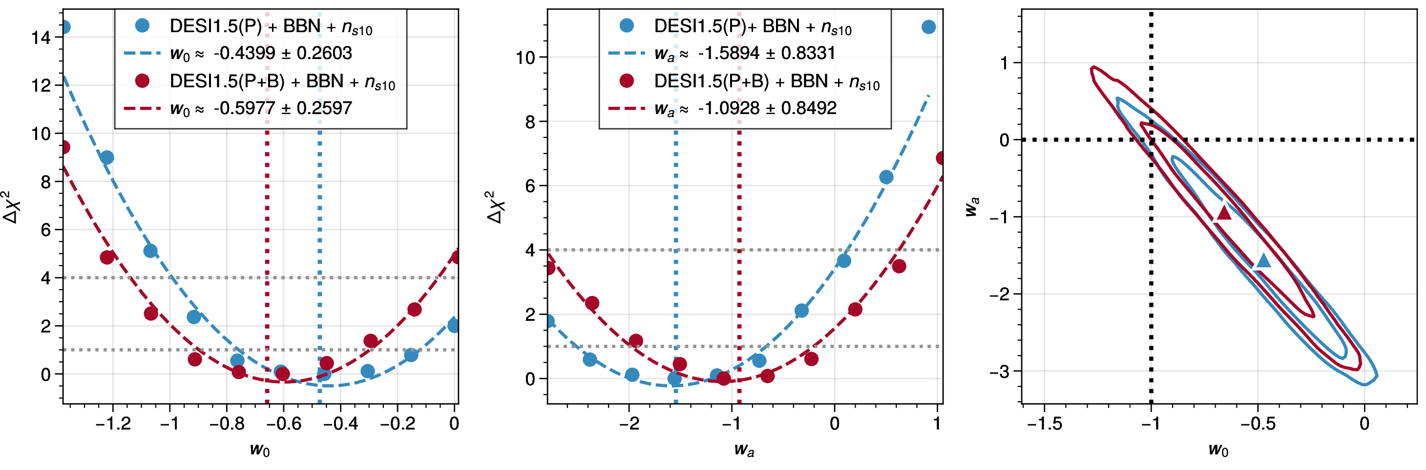
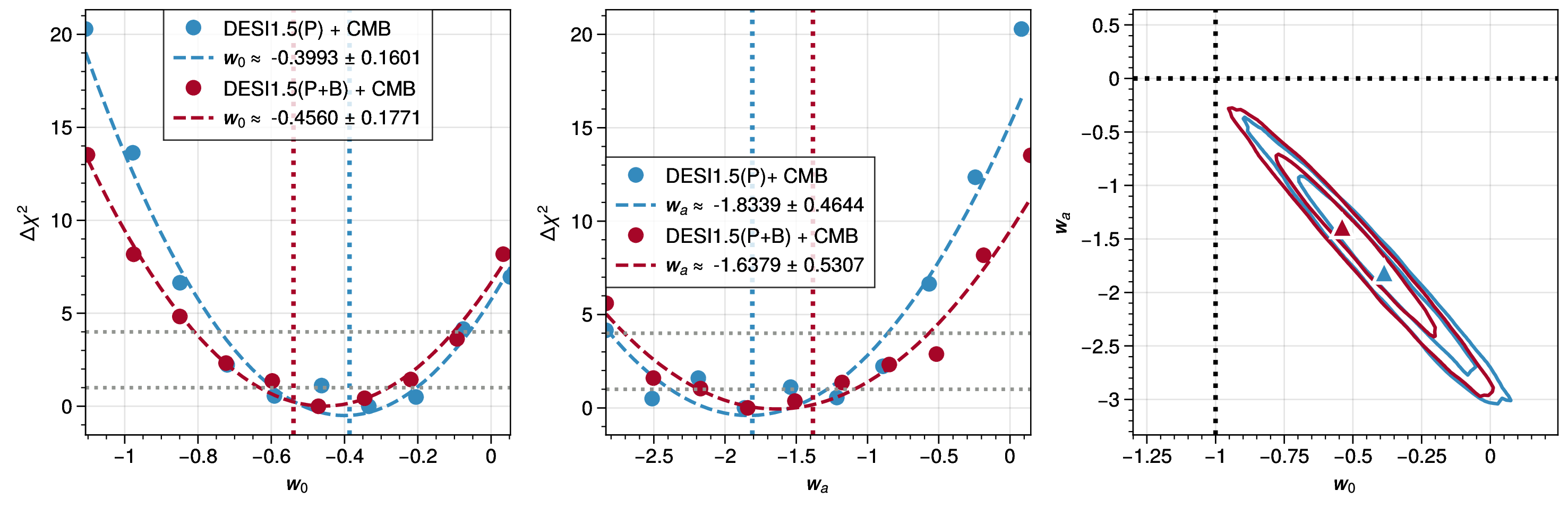
Figure 10: Binned \(\chi^2\) profiles for DESI-only (top) and DESI+CMB (bottom) showing the absence of parameter projection effects when using SF with and without the bispectrum. The dashed lines in the 1D profiles correspond to a parabolic fit to the binned minimum \(\chi^2\) (points). The right panel shows a 2D KDE-estimate of the binned \(\chi^2\) along with the MAP values (triangles). Notice that these align with the Bayesian contours in 5 confirming the absence of projection effects..
7 Author Affiliations↩︎
\(^{a}\)Institut de Ciències del Cosmos (ICCUB), Universitat de Barcelona (UB), c. Martí i Franquès, 1, 08028 Barcelona, Spain.
\(^{b}\)Departament de Fı́sica Quàntica i Astrofı́sica, Universitat de Barcelona, Martı́ i Franquès 1, E08028 Barcelona, Spain
\(^{c}\)Institut d’Estudis Espacials de Catalunya (IEEC), c/ Esteve Terradas 1, Edifici RDIT, Campus PMT-UPC, 08860 Castelldefels, Spain
\(^{d}\)Institució Catalana de Recerca i Estudis Avançats, Passeig de Lluı́s Companys, 23, 08010 Barcelona, Spain
\(^{e}\)Lawrence Berkeley National Laboratory, 1 Cyclotron Road, Berkeley, CA 94720, USA
\(^{f}\)Department of Physics, Boston University, 590 Commonwealth Avenue, Boston, MA 02215 USA
\(^{g}\)Dipartimento di Fisica “Aldo Pontremoli”, Università degli Studi di Milano, Via Celoria 16, I-20133 Milano, Italy
\(^{h}\)INAF-Osservatorio Astronomico di Brera, Via Brera 28, 20122 Milano, Italy
\(^{i}\)Department of Physics & Astronomy, University College London, Gower Street, London, WC1E 6BT, UK
\(^{j}\)Institute of Space Sciences, ICE-CSIC, Campus UAB, Carrer de Can Magrans s/n, 08913 Bellaterra, Barcelona, Spain
\(^{k}\)Institute for Computational Cosmology, Department of Physics, Durham University, South Road, Durham DH1 3LE, UK
\(^{l}\)Instituto de Fı́sica, Universidad Nacional Autónoma de México, Circuito de la Investigación Cientı́fica, Ciudad Universitaria, Cd. de México C. P. 04510, México
\(^{m}\)NSF NOIRLab, 950 N. Cherry Ave., Tucson, AZ 85719, USA
\(^{n}\)Department of Astronomy & Astrophysics, University of Toronto, Toronto, ON M5S 3H4, Canada
\(^{o}\)Department of Physics & Astronomy and Pittsburgh Particle Physics, Astrophysics, and Cosmology Center (PITT PACC), University of Pittsburgh, 3941 O’Hara Street, Pittsburgh, PA 15260, USA
\(^{p}\)University of California, Berkeley, 110 Sproul Hall #5800 Berkeley, CA 94720, USA
\(^{q}\)Institut de Física d’Altes Energies (IFAE), The Barcelona Institute of Science and Technology, Edifici Cn, Campus UAB, 08193, Bellaterra (Barcelona), Spain
\(^{r}\)Departamento de Física, Universidad de los Andes, Cra. 1 No. 18A-10, Edificio Ip, CP 111711, Bogotá, Colombia
\(^{s}\)Observatorio Astronómico, Universidad de los Andes, Cra. 1 No. 18A-10, Edificio H, CP 111711 Bogotá, Colombia
\(^{t}\)University of Virginia, Department of Astronomy, Charlottesville, VA 22904, USA
\(^{u}\)Fermi National Accelerator Laboratory, PO Box 500, Batavia, IL 60510, USA
\(^{v}\)Department of Astronomy, University of Texas at Austin, 2515 Speedway, TX 78712, USA
\(^{w}\)Institut d’Astrophysique de Paris. 98 bis boulevard Arago. 75014 Paris, France
\(^{x}\)IRFU, CEA, Université Paris-Saclay, F-91191 Gif-sur-Yvette, France
\(^{y}\)Center for Cosmology and AstroParticle Physics, The Ohio State University, 191 West Woodruff Avenue, Columbus, OH 43210, USA
\(^{z}\)Department of Physics, The Ohio State University, 191 West Woodruff Avenue, Columbus, OH 43210, USA
\(^{aa}\)The Ohio State University, Columbus, 43210 OH, USA
\(^{ab}\)Department of Physics, University of Michigan, 450 Church Street, Ann Arbor, MI 48109, USA
\(^{ac}\)University of Michigan, 500 S. State Street, Ann Arbor, MI 48109, USA
\(^{ad}\)Department of Physics, The University of Texas at Dallas, 800 W. Campbell Rd., Richardson, TX 75080, USA
\(^{ae}\)Department of Physics and Astronomy, University of California, Irvine, 92697, USA
\(^{af}\)Sorbonne Université, CNRS/IN2P3, Laboratoire de Physique Nucléaire et de Hautes Energies (LPNHE), FR-75005 Paris, France
\(^{ag}\)Departament de Física, Serra Húnter, Universitat Autònoma de Barcelona, 08193 Bellaterra (Barcelona), Spain
\(^{ah}\)Department of Physics and Astronomy, Siena University, 515 Loudon Road, Loudonville, NY 12211, USA
\(^{ai}\)Institute of Cosmology and Gravitation, University of Portsmouth, Dennis Sciama Building, Portsmouth, PO1 3FX, UK
\(^{aj}\)Departamento de Fı́sica, DCI-Campus León, Universidad de Guanajuato, Loma del Bosque 103, León, Guanajuato C. P. 37150, México
\(^{ak}\)Instituto Avanzado de Cosmologı́a A. C., San Marcos 11 - Atenas 202. Magdalena Contreras. Ciudad de México C. P. 10720, México
\(^{al}\)Department of Physics and Astronomy, University of Waterloo, 200 University Ave W, Waterloo, ON N2L 3G1, Canada
\(^{am}\)Perimeter Institute for Theoretical Physics, 31 Caroline St. North, Waterloo, ON N2L 2Y5, Canada
\(^{an}\)Waterloo Centre for Astrophysics, University of Waterloo, 200 University Ave W, Waterloo, ON N2L 3G1, Canada
\(^{ao}\)Instituto de Astrofísica de Andalucía (CSIC), Glorieta de la Astronomía, s/n, E-18008 Granada, Spain
\(^{ap}\)Departament de Física, EEBE, Universitat Politècnica de Catalunya, c/Eduard Maristany 10, 08930 Barcelona, Spain
\(^{aq}\)Department of Physics and Astronomy, Sejong University, 209 Neungdong-ro, Gwangjin-gu, Seoul 05006, Republic of Korea
\(^{ar}\)Abastumani Astrophysical Observatory, Tbilisi, GE-0179, Georgia
\(^{as}\)Department of Physics, Kansas State University, 116 Cardwell Hall, Manhattan, KS 66506, USA
\(^{at}\)Faculty of Natural Sciences and Medicine, Ilia State University, 0194 Tbilisi, Georgia
\(^{au}\)CIEMAT, Avenida Complutense 40, E-28040 Madrid, Spain
References↩︎
Hereafter, \(\mathcal{N}(\mu, \Sigma^2)\) denotes a normal distribution with mean \(\mu\) and (co)variance \(\Sigma^2\).↩︎
The definitions here omit the “BAO” superscript for brevity; the same forms hold for the SF compressed parameters. We use this \(q\)-notation for consistency with other DESI papers, though these are often referred to as \(\alpha\) in the literature.↩︎
We use the superscript “SF” to distinguish parameters derived from the full-shape ShapeFit analysis of pre-reconstructed catalogs from those labeled “BAO,” which are obtained by measuring only the BAO feature in the two-point correlation function of post-reconstructed catalogs. While covariant, these two measurements capture distinct cosmological information.↩︎
This is the amplitude parameter \(\require{physics} \sigma_{s8}^2 = \int_0^\infty P_{\rm lin}(k)W(ks8/(\,h^{-1}\,{\rm Mpc}))\dd^3k\), where \(W(k)\) is a top-hat filter, \(P_{\rm lin}\) is the Shapefit-modified linear power spectrum and \(s = r_s / r_S^{\rm fid}\) denotes the change in the filter scale due to the scalings \(q_{\rm iso,ap}\).↩︎
We approximate this frequentist figures from the difference in \(\chi^2\) from the two models.↩︎
We approximate the DIC value from the MCMC chains as \(\mathrm{DIC} \approx \langle\chi^2\rangle + \frac{1}{2}\mathrm{var}(\chi^2)\), where \({\rm var}(\chi^2)\) denotes the variance of the \(\chi^2\) values from the chain and \(\langle\chi^2\rangle\) their mean. This is a fair approximation when the posteriors do not show significant projection effects and are in general roughly Gaussian.↩︎
KATRIN cites upper bounds on a single neutrino mass of \(m_\beta < 0.31~\rm eV\;\text{90\% CL}\) (Feldman-Cousins) which we very approximately translate into a sum of masses of \(\sum m_\nu \lesssim 0.93~\rm eV\), very consistent with our constraint.↩︎