Augmenting Imaginary-Time Evolution with Local Geometric Information
June 22, 2026
Abstract
Imaginary-time evolution (ITE) underpins a broad family of algorithms for ground-state preparation in quantum simulation and quantum many-body physics. In these methods, convergence is governed by the energy variance of the instantaneous state, causing the flow to approach the ground state only asymptotically. We introduce an augmented imaginary-time evolution (AITE) framework that replaces the standard gradient flow on the energy landscape with a geometrically informed descent along locally optimal directions, which are identified by exploiting the higher-order statistical structure of the instantaneous energy distribution. The resulting flow strictly outperforms standard ITE throughout the entire evolution and exhibits two qualitatively distinct regimes: a superlinear convergence regime, followed by an extinction regime in which the energy error vanishes exactly at a finite imaginary time, in sharp contrast to the asymptotic exponential decay of ITE. Standard ITE is recovered in the zero-skewness limit of AITE, implying that the acceleration extends naturally across the broader ITE algorithmic family.
Imaginary-time evolution (ITE) is one of the central ideas behind modern approaches to low-energy many-body physics. Under the Wick rotation \(t \rightarrow -i\tau\), coherent dynamics are replaced by a non-unitary flow that exponentially suppresses excited-state components and drives the system toward its ground state [1]. This simple projection mechanism underlies a wide range of methods for ground-state preparation, thermal calculations, and spectral estimation in condensed-matter physics, quantum chemistry, and quantum field theory [2]–[4], and sits within a broader landscape of relaxation, filtering, and annealing methods that reach well beyond physics and chemistry [5].
While employing the same filtering principle, algorithms rooted in ITE take several distinct computational forms. In direct implementations, one approximates the non-unitary propagator \(\exp[-\tau \hat{H}]\), where \(\hat{H}\) is the Hamiltonian whose ground state is sought, iteratively, so that low-energy structure is progressively revealed by explicit imaginary-time cooling. In many-body settings, this includes product-formula propagation and tensor-network schemes, with block decimation and imaginary-time variational principles as natural matrix-product-state realizations [6]–[9]. Alternatively, stochastic projector methods realize the same spectral filtering statistically, through walker population dynamics or sampled paths whose branching and reweighting drive the dynamics toward low energy, as in diffusion Monte Carlo, auxiliary-field quantum Monte Carlo, and related projector approaches [10]–[13]. In yet another approach, variational formulations restrict the evolution to a tractable manifold of trial states, replacing exact propagation by projected descent within an ansatz state manifold [14]–[17]. Moreover, at the classical level, simulated annealing distills the same principle into a cooling schedule for combinatorial optimization [5], with applications ranging from circuit design to portfolio optimization [18]–[21].
Since the ITE propagator is non-unitary, it cannot be straightforwardly implemented as a quantum circuit, and this has led to several distinct quantum realizations of the same ITE objective. Some approaches stay as close as possible to the original flow, approximating short imaginary-time steps through implementable unitary updates or related hybrid constructions [22]. In contrast, others impose the evolution variationally in the form of a parameterized circuit [23]. Most recently, two wider viewpoints have become explicit. In one, the non-unitary propagator is treated as a particular instance of spectral filtering, placing ITE within a larger family of energy-selective transformations for low-energy state preparation [24]–[26]. In the other, cooling is reformulated in terms of structured flow equations, with double-bracket dynamics providing an alternative route to monotonic energy descent [27].
The geometric structure of ITE has also attracted growing attention. Brockett’s double-bracket flow established ITE as an isospectral gradient flow on the manifold of density operators [28], and the connection between ITE and gradient flow on the Riemannian manifold of quantum states (encoded in the quantum geometric tensor) has provided a natural language for understanding variational implementations and their convergence properties [29]. This geometric perspective has spurred an active line of research, establishing fidelity bounds for ground-state preparation and energy minimization, among other results [30]–[32].

Figure 1: Schematic comparison of standard imaginary-time evolution (ITE) and augmented imaginary-time evolution (AITE). a) In standard ITE, the energy distribution \(P(E)\) of the evolving state \(|\psi(\tau)\rangle\) shifts monotonically toward lower energies as \(\tau\) increases, converging to the ground state asymptotically as \(\tau \to \infty\). The convergence rate is governed solely by the energy variance. b) In AITE, the skewness of the instantaneous energy distribution is exploited to identify geometry-informed descent directions, yielding the ground state \(|\psi_{\text{GS}}\rangle\) at finite imaginary time \(\tau^*\). c) The key equations of AITE: the rate of energy decrease is given by \(\mathrm{Tr}[\hat{\chi}(\tau)\hat{O}(\tau)]\), where \(\hat{\chi}(\tau)\) is the double-bracket operator. The optimal operator \(\hat{O}(\tau) = |\lambda_-\rangle\langle\lambda_-|\) is the projector onto the lowest eigenvector of \(\hat{\chi}(\tau)\), projected onto the second-order Krylov subspace spanned by \(|\psi\rangle\) and \(\bar{H}|\psi\rangle\). d) AITE provides a universal upgrade of the ITE algorithmic family. Left: five main branches of ITE algorithms (Direct, Stochastic, Variational, Double-Bracket, and Spectral-Filter ITE) with examples of their representative implementations. Right: the corresponding AITE upgrades, obtained by the systematic substitution of \(\hat{H} \rightarrow \hat{H}_{\mathrm{A}}(\tau)\) in each branch..
Despite this remarkable breadth, the underlying dynamics of ITE have remained essentially unchanged across all these algorithmic branches. The literature has focused almost exclusively on finding efficient ways to implement the ITE flow rather than accelerating it. In almost all cases, this flow drives a monotonic energy decrease at a rate governed by the energy variance of the instantaneous state, and as a result, convergence can be prohibitively slow, depending sensitively on the energy gap and correlation length of the system. This intrinsic limitation has largely gone unaddressed, in some cases leaving a significant gap between the conceptual power of ITE and its practical computational efficiency.
In this work, we close this gap by introducing a systematic improvement of the ITE algorithm. Our approach builds on the double-bracket formulation of ITE [33], generalizing it to a significantly broader and more efficient family of descent flows. Rather than relying solely on local gradient information, our augmented imaginary-time evolution (AITE) explicitly incorporates the local geometric structure of the energy landscape, encoded in the higher-order statistical structure of the instantaneous energy distribution, to identify locally superlinear descent directions. This yields accelerated convergence and, quite remarkably, finite-time extinction of the energy error, in sharp contrast to the asymptotic exponential decay of standard ITE, as illustrated in Figs. 1a) and 1b). Crucially, since AITE subsumes ITE in its zero-skewness limit, this improvement propagates simultaneously across the broader family of algorithms inspired by ITE.
This paper is organized as follows. We first review the double-bracket formulation of quantum ITE and establish the geometric framework underlying our approach. We then introduce the main ingredients of AITE, derive the optimal descent direction, and discuss its implementation in both unitary and non-unitary forms, together with an analysis of its convergence properties. Next, we present numerical results for weakly and strongly correlated systems from condensed matter and quantum chemistry. We conclude with an outlook on extensions and potential applications of the AITE framework.
ITE and the Double-Bracket Formalism.— ITE prepares ground states by “cooling" an initial trial state \(\ket{\psi_0}\) through the continuous application of a non-unitary operator: \(\ket{\psi(\tau)} = e^{-\tau \hat{H}} \ket{\psi_0}\) [34]. Provided the initial trial state has a nonzero overlap with the ground state \(\ket{\psi_{\rm GS}}\) (i.e., \(|\langle \psi_{\rm GS} | \psi_0 \rangle| \neq 0\)), this evolution converges to the ground state in the limit of infinite imaginary time, \(\tau \to \infty\) [11], [35]. For practical purposes, it is convenient to work with the normalized state \[\begin{align} \label{normalizedstate} \ket{\psi(\tau)} = \frac{e^{-\tau \hat{H}}\ket{\psi_0}}{||e^{-\tau \hat{H}}\ket{\psi_0}||}. \end{align}\tag{1}\] This flow drives monotonic energy decrease at a rate set by the energy variance, notably, without critical slowing down [31]. As mentioned in the introduction, these imaginary-time dynamics underlie a remarkably rich family of algorithms for quantum simulation and optimization.
The state of Eq. 1 satisfies the norm-preserving differential equation \(\partial_\tau \ket{\psi(\tau)} = -\big(\hat{H} - E(\tau)\big)\ket{\psi(\tau)}\), where \(E(\tau)\) is the instantaneous energy. Recently, Ref. [33] observed that this equation can be written as \[\begin{align} \label{DB} \partial_\tau \ket{\psi(\tau)} = -[\hat{H}, \hat{\rho}(\tau)]\ket{\psi(\tau)}, \end{align}\tag{2}\] where \(\hat{\rho}(\tau) = \ket{\psi(\tau)}\bra{\psi(\tau)}\). This reformulation is significant for two reasons. First, the generator \([\hat{H}, \hat{\rho}(\tau)]\) is anti-Hermitian, so the flow admits a natural unitary realization. Second, this unitary structure enables efficient implementation on quantum hardware [36], [37].
AITE:— We generalize the flow of Eq. 2 by replacing \(\hat{\rho}(\tau)\) with a general projection operator \(\hat{\mathcal{O}}(\tau)\): \[\begin{align} \label{improvedDB} \partial_\tau \ket{\psi(\tau)} = -[\hat{H},\, \hat{\mathcal{O}}(\tau)]\ket{\psi(\tau)}. \end{align}\tag{3}\] Since \([\hat{H}, \hat{\mathcal{O}}(\tau)]\) is anti-Hermitian, the flow remains norm-preserving for any such choice. The condition for monotonic energy decrease, \(\partial_\tau \bra{\psi(\tau)}\hat{H}\ket{\psi(\tau)} \leq 0\), constrains the admissible choices of \(\hat{\mathcal{O}}(\tau)\). A direct calculation yields \[\begin{align} \label{functional} \partial_\tau \bra{\psi(\tau)}\hat{H}\ket{\psi(\tau)} = \mathrm{Tr}\!\left[\hat{\chi}(\tau)\,\hat{\mathcal{O}}(\tau)\right], \end{align}\tag{4}\] where \(\hat{\chi}(\tau) = -[\hat{H},[\hat{H},\hat{\rho}(\tau)]]\) is the double-bracket operator first introduced by Brockett [28], [38]. This operator encodes the local curvature of the energy landscape and coincides with the second imaginary-time derivative of the state under unitary dynamics. Finding a faster energy-decreasing update thus reduces to minimizing the linear functional in Eq. 4 over the space of admissible operators \(\hat{\mathcal{O}}(\tau)\). As shown in the Methods section, the minimizer \(\hat{\rho}^{\mathrm{A}}(\tau) = \operatorname*{argmin}_{\hat{\mathcal{O}}}\, \mathrm{Tr}\![\hat{\chi}(\tau)\,\hat{\mathcal{O}}]\), where the superscript \(A\) denotes the operator corresponding to AITE, steers the evolution in Eq. 3 along curvature-informed descent directions that are provably steeper than those of standard ITE.
Implementation of AITE:— We now discuss a practical choice of \(\hat{\rho}^{\mathrm{A}}(\tau)\) in order to implement AITE. While optimizing Eq. 4 over the full space of Hermitian operators is generally intractable, a natural and implementable solution emerges by restricting the search to a Krylov subspace—a well-established numerical framework that is, by no means, the only possible choice. Here, our choice is to work within the second-order Krylov subspace, \[\begin{align} \mathcal{S}_{\hat{M}}(\tau) = \{\ket{\psi(\tau)}, \ket{v_M(\tau)} \equiv \bar{M} \ket{\psi(\tau)}\}, \end{align}\] where \(\hat{M}\) is a Hermitian operator and \(\bar{M}\) is the centered operator \(\hat{M} - \bra{\psi(\tau)}\hat{M} \ket{\psi(\tau)}\). Within this subspace, the projection of the double-bracket operator \(\hat{\chi} (\tau)\) captures variations of the energy variance along directions orthogonal to \(\ket{\psi(\tau)}\). We now define the \(n\)th energy central moment as \(\mu_n(\tau) = \bra{\psi(\tau)}\bar{H}^n\ket{\psi(\tau)}\) and restrict the Krylov subspace to the choice \(\hat{M} \equiv \hat{H}\). The projected double-bracket operator takes the explicit form: \[\begin{align} \hat{\chi}(\tau)\big|_{\mathcal{S}_H(\tau)} = -2\mu_2(\tau) \begin{pmatrix} 1 & \frac{\kappa(\tau)}{2} \\ \frac{\kappa(\tau)}{2} & -1 \end{pmatrix}, \label{matrix} \end{align}\tag{5}\] where \[\begin{align} \kappa(\tau) = \frac{\mu_3(\tau)}{\mu_2^{3/2}(\tau)} . \end{align}\] is the instantaneous Fisher–Pearson skewness coefficient of the energy distribution [39]. This matrix admits a transparent statistical interpretation: the diagonal entries encode the energy variance \(\mu_2(\tau)\), while the off-diagonal entries are controlled by \(\kappa(\tau)\), which captures the asymmetry of the instantaneous energy distribution. While skewness is a well-established diagnostic of non-Gaussianity in quantitative finance and statistical learning [40]–[44], it has received comparatively little attention in the quantum simulation and ITE literature [45], [46]. Within \(\mathcal{S}_H(\tau)\) subspace, AITE thus naturally steers the descent using statistical information beyond the variance.
The eigenvalues of Eq. 5 are \[\begin{align} \lambda_\pm(\tau) = \pm 2\mu_2(\tau)\sqrt{1 + \frac{\kappa^2(\tau)}{4}}, \label{eq:flow95velocity} \end{align}\tag{6}\] with \(\lambda_-(\tau) \leq 0 \leq \lambda_+(\tau)\) for all \(\tau\). Restricting \(\hat{\mathcal{O}}(\tau)\) to rank-one projectors, the functional in Eq. 4 is minimized by the projector onto the eigenvector corresponding to \(\lambda_-(\tau)\), \[\begin{align} \hat{\rho}^{\mathrm{A}}(\tau) \equiv \ket{\lambda_-(\tau)}\bra{\lambda_-(\tau)}, \label{eq:rho95G} \end{align}\tag{7}\] where \(\ket{\lambda_-(\tau)} = \cos\phi(\tau)\ket{\psi(\tau)} + \sin\phi(\tau)\ket{v_H(\tau)}\). The mixing angle \(\phi(\tau)\) is a central quantity in our framework: it measures the deviation of the energy distribution from Gaussianity via the relation \(\tan(2\phi(\tau)) = \kappa(\tau)/2\). Notice that \(\kappa(\tau) = 0\) implies \(\phi(\tau) = 0\), and \(\hat{\rho}^{\mathrm{A}}(\tau)\) reduces to \(\hat{\rho}(\tau)\), recovering standard ITE. The structure of this optimized descent operator is illustrated schematically in Fig. 1c). Notably, extending the optimization to higher-order Krylov subspaces provides a systematic and principled route to capturing higher-order energy fluctuations (such as the kurtosis \(\mu_4\), and beyond), offering a natural hierarchy of improvements over standard ITE.
The descent rate corresponds to the lowest eigenvalue, and it satisfies \(\lambda_-(\tau) \leq -2\mu_2(\tau) = \mathrm{Tr}[\hat{\chi}(\tau)\,\hat{\rho}(\tau)]\) while demonstrating that ITE is provably suboptimal compared to AITE. The inequality is strict whenever \(\kappa(\tau) \neq 0\), that is, whenever the instantaneous energy distribution is asymmetric. This reveals a structural limitation of ITE algorithms that, to the best of our knowledge, has not been previously identified: conventional ITE implicitly assumes a symmetric energy distribution (i.e., \(\kappa(\tau) = 0\)), discarding non-Gaussian features and, most prominently, the skewness.
Non-unitary AITE.— A natural question is whether the generalized double-bracket flow of Eq. 3 with the minimizer obtained in Eq. 7 , admits a formulation as an augmented non-unitary ITE. The answer is affirmative: our framework offers considerable flexibility in designing augmented Hamiltonians \(\hat{H}_{\mathrm{A}}(\tau)\) such that the update rule \[\begin{align} \ket{\psi(\tau+\delta\tau)} = \frac{e^{-\delta\tau\hat{H}_{\mathrm{A}}(\tau)}\ket{\psi(\tau)}}{\|e^{-\delta\tau\hat{H}_{\mathrm{A}}(\tau)}\ket{\psi(\tau)}\|} \label{eq:ite95update} \end{align}\tag{8}\] reproduces, to first order in \(\delta\tau\), the same energy descent rate as the optimal double-bracket flow \(\lambda_-(\tau)\). A concrete example of such an augmented Hamiltonian is: \[\begin{align} \hat{H}_{\mathrm{A}}(\tau) = \cos(2\phi)\,\bar{H} + \frac{\sin(2\phi)}{2\sqrt{\mu_2(\tau)}}\,\bar{H}^2. \label{eq:effectiveH} \end{align}\tag{9}\] It is possible to construct augmented Hamiltonians by downfolding \(\bar{H}^2\) and retaining terms up to three-body interactions for electronic systems. In this case, as discussed in the Methods section, the prefactor of \(\bar{H}^2\) is modified accordingly, while the overall structure of the descent flow is preserved.
Convergence with power-law extinction.— We now investigate the late-time convergence structure of AITE. Standard ITE converges to the ground state with an energy error decaying as \(\varepsilon_{\rm ITE}(\tau) \sim e^{-2\Delta\tau}\), where \(\Delta = E_1 - E_{\rm GS}\) is the spectral gap. We show that AITE belongs to a qualitatively distinct convergence class. In the near-convergence regime \(\varepsilon_{\rm AITE}(\tau) \ll \Delta\), the quantum state is dominated by its ground-state component, so that \(\mu_2(\tau) \approx \Delta\varepsilon(\tau)\) and \(\mu_3(\tau) \approx \Delta^2\varepsilon(\tau)\). Using the AITE flow Eq. 6 yields \(\dot{\varepsilon}_{\rm AITE} = -2\Delta\varepsilon_{\rm AITE}\sqrt{1 + \Delta/4\varepsilon_{\rm AITE}}\), which makes explicit that AITE is strictly faster than ITE at every finite energy error \(\varepsilon\). The superlinear speedup factor \(\sqrt{1 + \Delta/4\varepsilon}\) diverges as \(\varepsilon \to 0\), reflecting increasingly aggressive acceleration near the ground state. Standard ITE, \(\dot{\varepsilon}_{\rm ITE} = -2\Delta\varepsilon_{\rm ITE}\), is recovered in the large-error limit \(\varepsilon \gg \Delta/4\), identifying it as the large-error asymptote of the augmented dynamics.

Figure 2: Energy error \(E(\tau)-E_{\rm GS}\) as a function of imaginary time \(\tau\) for ITE (black) and AITE (red) as predicted in Eq. 10 (with \(\Delta=1\) and \(\varepsilon_0=0.75\)). The main panel shows the error evolution on a logarithmic scale, with shaded regions identifying four dynamical regimes: the linear regime (\(\varepsilon\gg\Delta/4\), blue), the superlinear regime (\(\varepsilon\sim\Delta/4\), green), the power-law extinction regime (\(\varepsilon\ll\Delta/4\), red), and the asymptotic ITE regime. The dashed vertical line marks the finite extinction time \(\tau^*\) of AITE. The inset displays the same dynamics on a linear scale, highlighting the finite-time extinction of AITE in contrast to the asymptotic exponential decay of ITE..
The AITE flow admits the exact closed-form solution \[\begin{align} \varepsilon_{\rm AITE}(\tau) = \frac{\Delta}{4} \sinh^2\!\left( \sinh^{-1}\!\left(2\sqrt{\frac{\varepsilon_0}{\Delta}}\right) - \Delta\tau \right), \label{eq:exact95sol} \end{align}\tag{10}\] where \(\varepsilon_0 = \varepsilon(0)\) is the initial energy error. Surprisingly, unlike the ITE solution, which decays exponentially and reaches zero only as \(\tau \to \infty\), Eq. 10 vanishes exactly (i.e., \(\varepsilon_{\rm AITE}(\tau^*) = 0\)) at the finite extinction time: \[\begin{align} \tau^* = \frac{1}{\Delta} \sinh^{-1}\!\left(2\sqrt{\frac{\varepsilon_0}{\Delta}}\right). \label{eq:tau95star} \end{align}\tag{11}\] Expanding the energy error around \(\tau^*\) and using \(\sinh(x) \approx x\) for small \(x\), Eq. 10 gives \[\begin{align} \label{eq:power95law95extinction} \varepsilon_{\rm AITE}(\tau) \approx \frac{\Delta^3}{4}(\tau^* - \tau)^2, \end{align}\tag{12}\] a power-law extinction with exponent \(2\). This stands in sharp contrast to the exponential tail of ITE and establishes that the two methods belong to provably distinct convergence classes. The finite-time power-law extinction of AITE is reminiscent of finite-time extinction in nonlinear diffusion equations, such as the fast diffusion equation in porous media [47], where solutions to \(\dot{\varepsilon} = -c\varepsilon^\alpha\) with \(\alpha < 1\) are known to reach zero in finite time. The near-ground-state AITE dynamics fall precisely into this class with \(\alpha = \tfrac{1}{2}\).
Finally, from Eq. 11 , the extinction time \(\tau^*\) depends on the initial error only through \(\sinh^{-1}(2\sqrt{\varepsilon_0/\Delta})\). In the large-error regime \(\varepsilon_0 \gg \Delta\), using \(\sinh^{-1}(x) \approx \ln(2x)\) for \(x \gg 1\), this gives \(\tau^* \approx ({1}/{2\Delta})\ln({4\varepsilon_0}/{\Delta})\) so \(\tau^*\) grows only logarithmically with \(\varepsilon_0\). This is to be compared with standard ITE, where the time to reach a fixed target precision \(\varepsilon_*\) is \(\tau_{\mathrm{ITE}}(\varepsilon_*) = ({1}/{2\Delta})\ln({\varepsilon_0}/{\varepsilon_*})\), which diverges as \(\varepsilon_* \to 0\) for any fixed \(\varepsilon_0\). In AITE, by contrast, the time to reach any target precision is bounded from above by \(\tau^*\), which is independent of \(\varepsilon_*\) and grows only as \(\ln(\varepsilon_0/\Delta)\). Although the analysis above focuses on the near-convergence regime, where the state is dominated by its ground-state component, the result remains valid for arbitrary state populations. The proof of the general case is deferred to the Methods section.
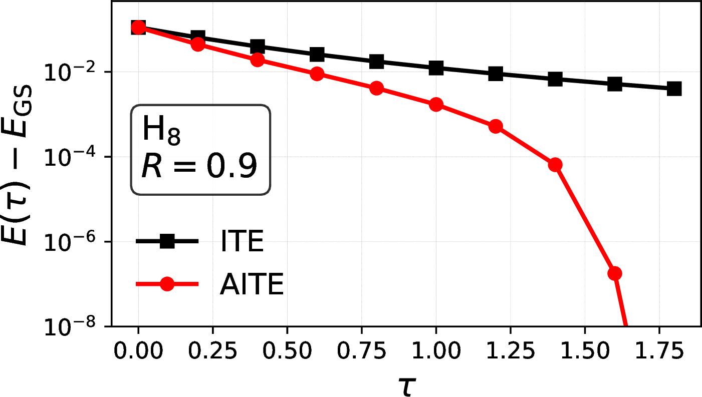
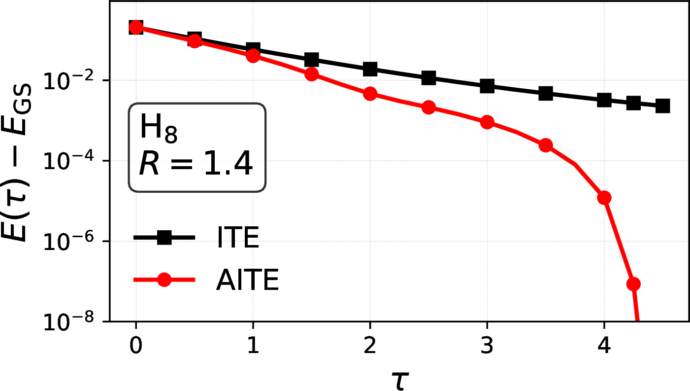
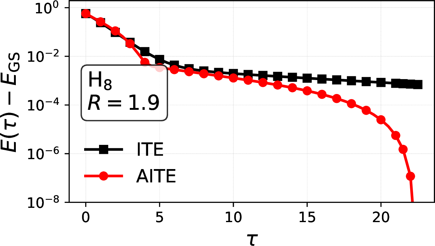
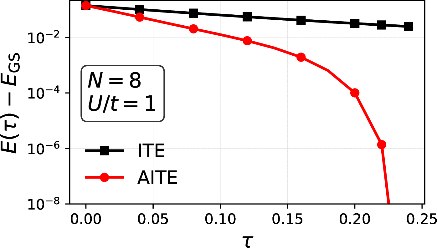
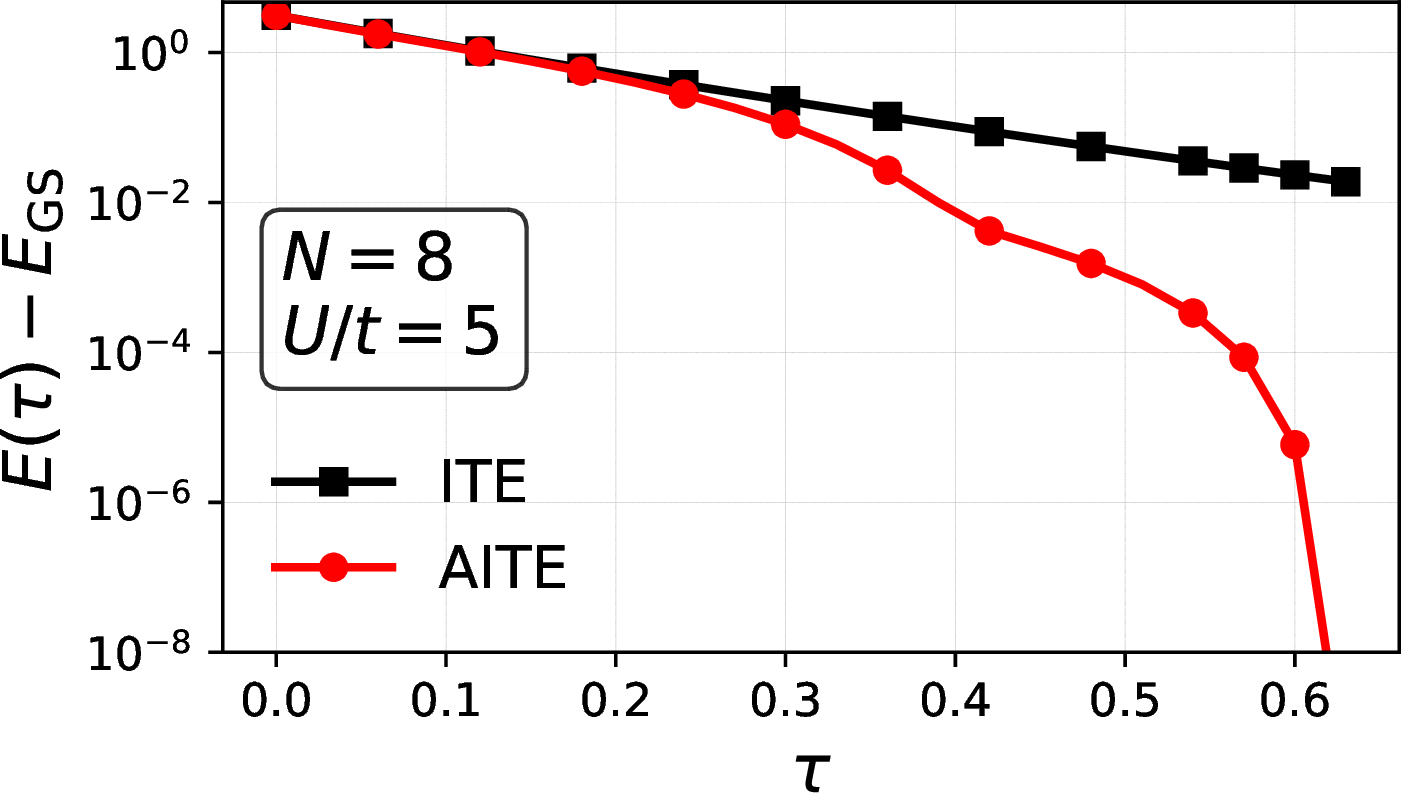
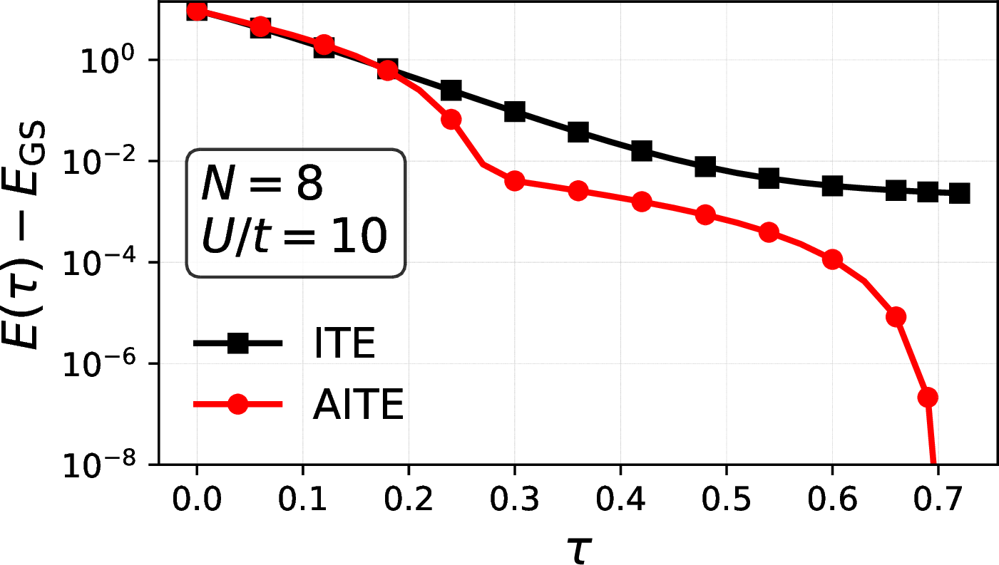
Figure 3: Energy error \(E(\tau)-E_{\rm GS}\) as a function of imaginary time \(\tau\) for equidistant \(\mathrm{H}_8\) (upper panels) and the one-dimensional Fermi-Hubbard model at half filling with \(N=8\) sites and open boundary conditions (lower panels). Within each row, the interatomic spacing \(R\) (\(\mathrm{H}_8\)) and interaction strength \(U/t\) (Hubbard) increase from left to right. Results are shown for ITE and AITE. In all cases, the initial trial state corresponds to the Hartree–Fock state..
In summary, the fundamental asymmetry between the two algorithms is this: in ITE, the convergence time grows without bound as the target precision is tightened, whereas in AITE it is determined solely by the initial energy error and the spectral gap, independent of the target precision altogether. As illustrated in Fig. 2, AITE exhibits three distinct dynamical regimes: a linear regime, in which the descent closely tracks standard ITE; a superlinear regime, in which the non-Gaussian skewness begins to dominate and drive the AITE dynamics; and a power-law extinction regime, in which the energy error vanishes exactly at the finite time \(\tau^*\), while ITE continues its asymptotic exponential decay.
Numerical experiments.— We benchmark AITE across both weakly and strongly correlated regimes of two model systems in condensed matter and quantum chemistry. Fig. 3 compares AITE to ITE for the equidistant hydrogen chain \(\mathrm{H}_8\) at three interatomic distances (\(R = 0.9, 1.4, 1.9\) Å) and the eight-site one-dimensional Fermi-Hubbard model with open boundary conditions at half filling at three interaction strengths (\(U/t = 1, 5, 10\)). In both cases, we use the Hartree–Fock state as the initial state. We find that across all geometries and interaction strengths, the energy error exhibits the three dynamical regimes predicted analytically above: the linear, superlinear, and power-law extinction regimes. The consistent acceleration across different correlation regimes corroborates the central role of non-Gaussian features of the instantaneous energy distribution in driving convergence beyond the exponential barrier of standard ITE.
Heuristics for higher momenta.— The skewness appearing in Eq. 5 probes non-Gaussian structure in the energy distribution that is costly to access in practice, both on near-term quantum hardware [45], [48] and in classical implementations, as it requires estimating three-fold correlations of the Hamiltonian. Below, we address this by proposing a practical strategy to reduce computational overhead without sacrificing the superlinear convergence of AITE.
We introduce a mean-field approximation \(\langle \hat{H}^3\rangle \approx \langle \hat{H}^2\rangle\langle \hat{H}\rangle\), which decouples three-point correlations into products of lower-order expectation values, yielding the mean-field skewness \(\kappa_{\rm MF}(\tau) \approx -2E(\tau)/\sqrt{\mu_2(\tau)}\). Since \(E(\tau) > E_{\rm GS}\) throughout the descent, \(\kappa_{\mathrm{MF}}(\tau)\) is strictly negative, consistent with the energy distribution being left-skewed as the state approaches the ground state. Crucially, this expresses the third moment entirely in terms of first- and second-order expectation values of \(\hat{H}\), which are directly accessible from energy and variance measurements without additional computational overhead. In addition, \(\kappa_{\rm MF}(\tau)\) becomes exact whenever the energy distribution is sharply concentrated around a single eigenvalue. This is precisely the regime that is approached as the algorithm converges, so the mean-field approximation improves in accuracy throughout the descent and is asymptotically exact at convergence. It therefore provides a computationally efficient and systematically improvable entry point for AITE.
Fig. 4 compares the performance of our heuristic approximation to the skewness against standard ITE and AITE, and also includes a Krylov-subspace energy estimate in which, at each imaginary-time step, the energy is optimized within the second-order Krylov subspace \(\mathcal{S}_H(\tau)\) generated by the instantaneous state. We note that this Krylov energy estimate is upper-bounded by the AITE energy and comes essentially for free, as it requires only the expectation values \(\langle \hat{H}^k \rangle\) with \(k \leq 3\), all of which are already evaluated as part of the AITE flow.
At early times, when the energy distribution remains approximately Gaussian, and the skewness is small, \(|{\kappa(\tau)}/{2}| \lesssim 1\), the four curves follow closely similar paths. Once the skewness becomes significant, however, AITE enters the superlinear convergence regime that standard ITE cannot access. Remarkably, the mean-field approximation \(\kappa_{\rm MF}\) captures the skewness with sufficient accuracy that the resulting approximate AITE retains the same convergence characteristics as the exact method, making it a practical alternative that avoids the explicit measurement of third-order expectation values. We note that the strong performance of \(\kappa_{\rm MF}\) is particularly pronounced at equilibrium geometries. Constructing improved heuristics for the skewness in more general settings is a natural direction for future work.
As expected, the Krylov estimate yields even lower energies than AITE throughout the evolution, sometimes improving it by up to multiple orders of magnitude. This suggests that combining Krylov-subspace energy optimization with the AITE flow provides a natural route to further accelerating convergence beyond what either approach achieves independently.
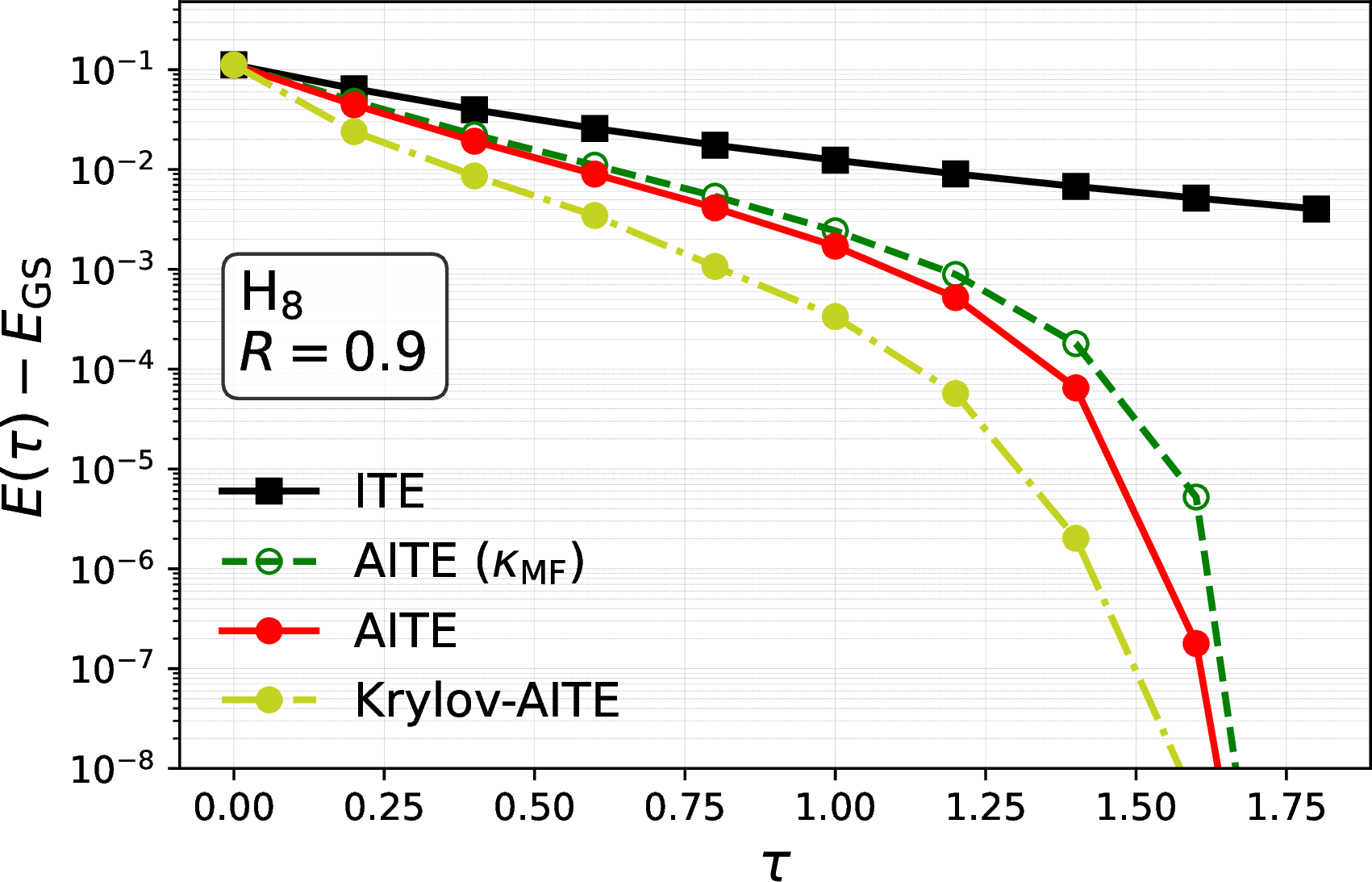
Figure 4: Energy error \(E(\tau) - E_{\rm GS}\) as a function of imaginary time \(\tau\) for standard ITE (black), AITE (red), AITE using the mean-field skewness approximation \(\kappa_{\mathrm{MF}}\) (green), and the Krylov-subspace energy estimator for AITE (yellow), applied to the hydrogen chain H\(_8\)..
Discussion.— We have introduced an augmented imaginary-time evolution (AITE) framework that replaces the standard gradient flow on the energy landscape with a geometrically informed descent along locally optimal directions. The resulting flow strictly outperforms standard ITE and exhibits three qualitatively distinct regimes: a linear and a superlinear convergence regimes, followed by a finite-time extinction regime.
Since AITE recovers standard ITE as its zero-skewness limit, the acceleration is not tied to any particular implementation. As sketched in Fig. 1d), the substitution \(\hat{H} \rightarrow \hat{H}_{\mathrm{A}}\) offers a natural upgrade path for every branch of the ITE algorithmic family, requiring targeted modifications to the underlying algorithmic structure. In fact, beyond requiring statistical information of the instantaneous state, AITE amounts to replacing the standard propagator with an augmented one that resembles a Gaussian filter [49], making it directly accessible within existing implementations. In direct ITE, the imaginary-time propagator \(\exp[-\tau\hat{H}]\) can be replaced by \(\exp[-\tau\hat{H}_{\mathrm{A}}]\), yielding a geometrically informed filter that reaches the ground state at finite time. In stochastic ITE (auxiliary-field quantum Monte Carlo [13], diffusion Monte Carlo [50], and full configuration-interaction quantum Monte Carlo [51]), the effective Hamiltonian governing the importance-sampling weights can be replaced by its augmented counterpart, biasing the walker dynamics toward steeper descent directions. In variational ITE (variational quantum imaginary-time evolution [23], variational Monte Carlo [52], neural quantum states [53], and contracted variational eigensolvers [54], [55]), the gradient vector \(C_i(\theta)\) can be replaced by its augmented counterpart \(C_i^{\mathrm{A}}(\theta)\), steering the parameter flow along provably steeper descent directions without changing the ansatz or the circuit structure. In double-bracket ITE [33], the bracket generator \([\hat{H}, \hat{\rho}]\) can be promoted to \([\hat{H}, \hat{\rho}^{\mathrm{A}}]\) or, alternatively, \([\hat{H}_{\mathrm{A}}, \hat{\rho}]\), accelerating the flow while preserving its unitary structure. Finally, in spectral-filter ITE (quantum singular value transformation [56] and quantum eigenvalue transformation of unitaries [57]), the polynomial filter applied to \(\hat{H}\) can be recentered around \(\hat{H}_{\mathrm{A}}\), sharpening the spectral projection and reducing the required polynomial degree for a fixed target precision.
This apparent accessibility comes with method-dependent overheads, set by whether a given formulation only requires moments of the instantaneous state or must explicitly realize the augmented propagator. The moment-estimation cost is common to all variants of AITE: \(\langle \hat{H}^2\rangle\) is essentially free in repeated-action methods, since \(\langle \hat{H}^2\rangle=|\hat{H}|\psi\rangle|^2\), but becomes representation-limited in local-compilation approaches such as ITPP, QITE, MITE and PITE, where \(\hat{H}^2\) generates pairwise products of elementary Hamiltonian terms; the moment \(\langle \hat{H}^3\rangle\), which can be avoided by using the mean-field skewness heuristic, produces the corresponding triple products [22], [58]–[63]. In tensor-network formulations, the same proliferation appears as an increase of the relevant MPO objects from \(D\) to \(D^2\) or \(D^3\) before compression [64], [65], while LCU constructions inherit enlarged decompositions and normalization factors [66], [67]. Spectral-transform methods are exceptional in that these powers remain low-degree functions of the spectrum; in QSVT, \(\langle \hat{H}^2\rangle\) can even be extracted directly from a block-encoding ancilla population, although the analogous shortcut is absent for the odd moment \(\langle \hat{H}^3\rangle\) [57], [68]. In stochastic and variational projector methods the limitation is mainly statistical rather than algebraic: VMC and neural quantum states can estimate \(\langle \hat{H}^2\rangle\) from squared local energies, whereas \(\langle \hat{H}^3\rangle\) requires access to \((\hat{H}^2\psi(x))/\psi(x)\); AFQMC, DMC, FCIQMC and PIGS instead incur purer estimators, longer back-propagation or forward-walking procedures, midpoint insertions, or higher-hop determinant connectivity [12], [51], [69]–[72]. This broadly shared moment overhead should be separated from the stronger requirement of implementing \(\exp[-\tau \hat{H}_A]\), which arises only in formulations whose primitive is an explicit projector or spectral filter. Such propagation is benign for state-vector or Krylov evolution, natural in QSVT/QETU as the scalar filter \(\exp[-\tau(a_1x+a_2x^2)]\), but substantially more costly for local, LCU, and tensor-network representations, where the quadratic products become part of the generator itself [57]–[59], [64], [66]–[68]. It is least natural for stochastic projector algorithms, whose native Hubbard–Stratonovich, drift–diffusion–branching or short-time-action structures are not generically preserved by replacing \(\hat{H}\) with \(\hat{H}_A\) [12], [69], [71], [72]. In contrast, variational and double-bracket formulations need not apply \(\exp[-\tau\hat{H}_A]\) as a primitive; the augmented Hamiltonian enters instead through projected gradients, local estimators, or commutator generators [23], [33], [70], [73]. Detailed implementations of the individual AITE variants and optimized cost analyses beyond the qualitative considerations presented here are left to future work.
Acknowledgments.— We thank Aeishah Ameera Anuar, Dimitri Pimenov, and Manuel Algaba for insightful discussions, and Pietropaolo Frisoni for carefully checking our derivations and identifying a sign error in the mixing-angle relation.
Methods↩︎
Here we present a detailed account of the construction of the double-bracket flow in experimentally accessible subspaces, the optimization of the descent direction, and the construction of the augmented Hamiltonian \(\hat{H}_{\mathrm{A}}(\tau)\). We also generalize our finite-extinction proof.
Projected double-bracket flow.— Let \(\hat{M}\) be a Hermitian operator and consider the associated two-dimensional Krylov subspace \[\begin{align} \mathcal{S}_M(\tau) = \mathrm{span} \left\{\ket{\psi(\tau)}, \ket{v_M(\tau)} \equiv \frac{\bar{M}\ket{\psi(\tau)}}{\sqrt{\mu_2^M(\tau)}}\right\}, \end{align}\] where \(\bar{M} \equiv \hat{M} - M(\tau)\) is the centered operator with \(M(\tau) = \bra{\psi(\tau)}\hat{M}\ket{\psi(\tau)}\), and \(\mu_n^M(\tau) \equiv \bra{\psi(\tau)}\bar{M}^n\ket{\psi(\tau)}\) is the \(n\)th central moment of \(\hat{M}\) in the state \(\ket{\psi(\tau)}\). The operator of core interest is the double commutator \(\hat{\chi}(\tau) \equiv -\bigl[\hat{H},\bigl[\hat{H},\hat{\rho}(\tau)\bigr]\bigr]\), \(\hat{\rho}(\tau) \equiv \ket{\psi(\tau)}\bra{\psi(\tau)}\). Restricting \(\hat{\chi}(\tau)\) to \(\mathcal{S}_M(\tau)\) yields the matrix representation \(\chi(\tau) \equiv \hat{\chi}(\tau)\big|_{\mathcal{S}_M(\tau)}\), \[\begin{align} \label{matrixchi} \chi(\tau) = \begin{pmatrix} \bra{\psi(\tau)}\hat{\chi}\ket{\psi(\tau)} & \bra{\psi(\tau)}\hat{\chi}\ket{v_M(\tau)} \\[6pt] \bra{v_M(\tau)}\hat{\chi}\ket{\psi(\tau)} & \bra{v_M(\tau)}\hat{\chi}\ket{v_M(\tau)} \end{pmatrix}. \end{align}\tag{13}\] We now specialize to \(\hat{M} = \hat{H}\) and, for brevity, write \(\mu_n(\tau) \equiv \mu_n^H(\tau)\). In this case, the restriction of the double commutator to \(\mathcal{S}_H(\tau)\) takes the form of the matrix presented in Eq. 5 .
We aim to minimize the linear functional \[\begin{align} \mathcal{F}_{\chi(\tau)}[\hat{\mathcal{O}}] \equiv Tr\bigl[\chi(\tau)\,\hat{\mathcal{O}}\bigr] \end{align}\] over the set of (Hermitian) projectors acting on \(\mathcal{S}_H(\tau)\). Since \(\mathcal{S}_H(\tau)\) is two-dimensional, the minimum is attained within the set of rank-\(1\) projectors \(\hat{\mathcal{O}} = \ket{\phi}\bra{\phi}\), for which the functional reduces to the Rayleigh quotient \[\begin{align} \mathcal{F}_{\chi(\tau)}[\ket{\phi}\bra{\phi}] = Tr\bigl[\chi(\tau)\ket{\phi}\bra{\phi}\bigr] = \bra{\phi}\chi(\tau)\ket{\phi}. \end{align}\] By the min-max theorem, the minimum of the Rayleigh quotient over all unit vectors \(\ket{\phi} \in \mathcal{S}_H(\tau)\) is the smallest eigenvalue of \(\chi(\tau)\), attained at the corresponding eigenvector. The global minimum over all Hermitian projectors on \(\mathcal{S}_H(\tau)\) is therefore \[\begin{align} \min_{\hat{\mathcal{O}}}\,\mathcal{F}_{\chi(\tau)}[\hat{\mathcal{O}}] = -\sqrt{4\mu_2^2(\tau)\big[1 + \tfrac14\kappa^2(\tau)\big]}, \label{eq:bound} \end{align}\tag{14}\] and the minimum is attained uniquely at the rank-one projector \[\begin{align} \hat{\rho}^{\mathrm{A}}(\tau) = \ket{\lambda_-(\tau)}\bra{\lambda_-(\tau)}, \end{align}\] where \(\ket{\lambda_-(\tau)} = \cos(\phi(\tau))\ket{\psi(\tau)} + \sin(\phi(\tau))\ket{v_H(\tau)}\). The mixing angle \(\phi(\tau)\) is determined by the eigenvalue equation for \(\chi(\tau)\). A direct application of the double-angle formula yields \(\tan\bigl(2\phi(\tau)\bigr) = \kappa(\tau) /2\).
Generalized Hamiltonians.— We now seek a generalized Hamiltonian of the form \[\label{eq:K-ansatzMethod} \hat{H}_{\mathrm{A}}(\tau) = a_1\bar{H} + a_2\bar{H}^2, \qquad a_1,a_2\in\mathbb{R},\tag{15}\] such that normalized imaginary-time evolution under \(\hat{H}_{\mathrm{A}}(\tau)\) reproduces, to leading order in imaginary time, the target double-bracket flow: \[\label{eq:goal} \frac{e^{-\beta \hat{H}_{\mathrm{A}}(\tau)}|\psi\rangle}{\|e^{-\beta \hat{H}_{\mathrm{A}}(\tau)}|\psi\rangle\|} \approx e^{-s[\hat{H},\hat{\rho}^{\mathrm{A}}(\tau)]}|\psi\rangle.\tag{16}\] A direct computation yields the exact decomposition \[\label{eq:HO-decompMethod} [\hat{H},\hat{\rho}^{\mathrm{A}}(\tau)]|\psi\rangle = \Omega_{\rm eff}(\phi)\,|v_H\rangle + \frac{\sin(2\phi)}{2\sqrt{\mu_2}}\ket{\perp},\tag{17}\] where \(\Omega_{\rm eff}(\phi) = \sqrt{\mu_2}\cos(2\phi) + \frac{\mu_3}{2\mu_2}\sin(2\phi)\), and \[\begin{align} \ket{\perp} = \bar{H}^2|\psi\rangle - \mu_2|\psi\rangle - \frac{\mu_3}{\sqrt{\mu_2}}|v_H\rangle. \end{align}\] Note that \(\ket{\perp}\) is not normalized: \(\|\ket{\perp}\|^2 = \mu_4 - \mu_2^2 - \mu_3^2/\mu_2\).
The target state to first order in \(s\) is therefore \[\label{eq:targetMethod} e^{-s[\hat{H},\hat{\rho}^{\mathrm{A}}(\tau)]}|\psi\rangle = |\psi\rangle - s\,\Omega_{\rm eff}(\phi)\,|v_H\rangle - \frac{s\sin(2\phi)}{2\sqrt{\mu_2}}\ket{\perp} + \mathcal{O}(s^2).\tag{18}\] Expanding \(e^{-\beta \hat{H}_{\mathrm{A}}}\) and normalizing: \[\label{eq:ITE-expandMethod} \frac{e^{-\beta \hat{H}_{\mathrm{A}}}|\psi\rangle}{\|e^{-\beta \hat{H}_{\mathrm{A}}}|\psi\rangle\|} \approx |\psi\rangle - \beta\,\bigl(\hat{H}_{\mathrm{A}} - \langle \hat{H}_{\mathrm{A}}\rangle_\psi\bigr)|\psi\rangle + \mathcal{O}(\beta^2).\tag{19}\] Matching Eq. 19 to Eq. 18 requires equating components along \(|v_H\rangle\) and \(\ket{\perp}\) separately. Projecting onto \(|v_H\rangle\) and using the ansatz 15 gives \[\label{eq:match-e1-explicitMethod} \frac{\beta}{\sqrt{\mu_2}}\bigl(a_1\mu_2 + a_2\mu_3\bigr) = s\,\Omega_{\rm eff}(\phi),\tag{20}\] where we used \(\bra{v_H}\bar{H}|\psi\rangle = \sqrt{\mu_2}\) and \(\bra{v_H}\bar{H}^2|\psi\rangle = \mu_3/\sqrt{\mu_2}\). Projecting onto \(\ket{\perp}\) and using \(\bra{\perp}\psi\rangle = 0\) gives \[\label{eq:match-perp-explicitMethod} \beta a_2\,\|\ket{\perp}\|^2 = \frac{s\sin(2\phi)}{2\sqrt{\mu_2}}\,\|\ket{\perp}\|^2,\tag{21}\] from which \(a_2 = (s/\beta)\sin(2\phi)/(2\sqrt{\mu_2})\). Finally, substituting into Eq. 20 yields \(a_1 = \frac{s}{\beta}\,\cos(2\phi)\).
Alternatively, one can construct a different augmented Hamiltonian of the form \[\begin{align} \hat{H}'_{\mathrm{A}}(\tau) = a'_1\bar{H} + a'_2\bar{K}, \label{eq:altH} \end{align}\tag{22}\] where \(\hat{K}\) is an operator obtained by downfolding \(\bar{H}^2\) and retaining terms up to a prescribed many-body rank, and \(a'_1\), \(a'_2\) are coefficients determined by the same matching condition as before. This provides a computationally cheaper alternative to the full \(\bar{H}^2\).

Finite-time extinction beyond the two-level regime.— The closed-form solution of Eq. 10 and the extinction time of Eq. 11 were derived in the near-convergence regime, where the state is dominated by its ground-state component and the moments reduce to \(\mu_2\simeq\Delta\varepsilon\), \(\mu_3\simeq\Delta^2\varepsilon\). We now show that finite-time extinction is not an artifact of this reduction.
Lemma 1 (Moment bounds). Let \(\hat{H} = \sum_k E_k \ket{E_k}\bra{E_k}\) have a nondegenerate ground state, spectral gap \(\Delta = E_1-E_{\rm GS}>0\), and let \(\ket{\psi}\) be any normalized state with energy error \(\varepsilon=\langle\hat{H}\rangle-E_{\rm GS}\), \(0<\varepsilon<\Delta\). Write \(\Delta_k=E_k-E_{\rm GS}\) and \(p_k=|\braket{k}{\psi}|^2\). Then \[\mu_2 \,\ge\, \varepsilon\,(\Delta-\varepsilon), \qquad \mu_3 \,\ge\, (\Delta-\varepsilon)\,\mu_2 \,-\, p_0\,\varepsilon^2\Delta . \label{eq:momentbounds}\qquad{(1)}\]
Proof. Since \(\Delta_k\ge\Delta\), \(\sum_k p_k\Delta_k^2\ge\Delta\sum_{k\ge1}p_k\Delta_k=\Delta\varepsilon\), and \(\mu_2=\sum_k p_k\Delta_k^2-\varepsilon^2\ge\varepsilon(\Delta-\varepsilon)\). For the third moment, split off the ground-state term: \(\mu_3=-p_0\varepsilon^3+\sum_{k\ge1}p_k(\Delta_k-\varepsilon)^3\). For \(k\ge1\) and \(\varepsilon<\Delta\) one has \(\Delta_k-\varepsilon\ge\Delta-\varepsilon>0\), hence \((\Delta_k-\varepsilon)^3\ge(\Delta-\varepsilon)(\Delta_k-\varepsilon)^2\), and \(\sum_{k\ge1}p_k(\Delta_k-\varepsilon)^2=\mu_2-p_0\varepsilon^2\). Therefore, \(\mu_3\ge(\Delta-\varepsilon)(\mu_2-p_0\varepsilon^2)-p_0\varepsilon^3 =(\Delta-\varepsilon)\mu_2-p_0\varepsilon^2\Delta\). ◻
Theorem 2 (Finite-time extinction). Along the exact AITE flow, \(\dot{\varepsilon}=-\sqrt{4\mu_2^2+\mu_3^2/\mu_2}\), the energy error obeys, for all \(\varepsilon\in(0,\Delta/4]\), \[\dot{\varepsilon}\;\le\; -\,\frac{5}{16}\,\Delta^{3/2}\sqrt{\varepsilon}\,. \label{eq:sqrtbound}\qquad{(2)}\] Consequently, once a trajectory satisfies \(\varepsilon(\tau_1)=\varepsilon_1\le\Delta/4\), it reaches \(\varepsilon=0\) exactly, at a time \[\tau^* \;\le\; \tau_1+\frac{32}{5}\, \frac{1}{\Delta}\sqrt{\frac{\varepsilon_1}{\Delta}} \;\le\; \tau_1+\frac{16}{5\Delta}\,. \label{eq:tstarbound}\qquad{(3)}\] Moreover, any trajectory with \(\varepsilon(0)=\varepsilon_0<\Delta\) enters this basin in the finite time \(\tau_1\le\frac{1}{2\Delta}\ln\!\big(\tfrac{3\varepsilon_0}{\Delta-\varepsilon_0}\big)\).
Proof. Fix \(\varepsilon\le\Delta/4\) and abbreviate \(x=\varepsilon/\Delta\in(0,\tfrac14]\). The rate obeys \(|\dot{\varepsilon}|=\sqrt{4\mu_2^2+\mu_3^2/\mu_2}\ge|\mu_3|/\sqrt{\mu_2} \ge\mu_3/\sqrt{\mu_2}\) unconditionally. By Lemma 1 and \(p_0\le1\), \[\begin{align} \frac{\mu_3}{\sqrt{\mu_2}} \;\ge\; (\Delta-\varepsilon)\sqrt{\mu_2}\,-\,\frac{\varepsilon^2\Delta}{\sqrt{\mu_2}} . \end{align}\] The right-hand side is increasing in \(\mu_2\) (i.e., its derivative, \((\Delta-\varepsilon)/2\sqrt{\mu_2}+\varepsilon^2\Delta/2\mu_2^{3/2}\), is positive) so it is minimized at the smallest variance, \(\mu_2=\varepsilon(\Delta-\varepsilon)\) from Lemma 1, giving \[\begin{align} \frac{\mu_3}{\sqrt{\mu_2}} &\ge\;(\Delta-\varepsilon)^{3/2}\sqrt{\varepsilon} -\frac{\Delta\,\varepsilon^{3/2}}{\sqrt{\Delta-\varepsilon}} \nonumber \\ &=\Delta^{3/2}\sqrt{\varepsilon}\;\frac{1-3x+x^2}{\sqrt{1-x}} . \end{align}\] On \((0,\tfrac14]\), \(1-3x+x^2\) is decreasing and \(\sqrt{1-x}\le1\), hence the prefactor is bounded below by \(1-3\cdot\tfrac14+\tfrac1{16}=\tfrac{5}{16}\). This proves Eq. ?? . Setting now \(u=\sqrt{\varepsilon}\), inequality ?? reads \(\dot{u}\le-\tfrac{5}{32}\Delta^{3/2}\), so \(u\) reaches zero no later than \(\tau^* = \tau_1+\tfrac{32}{5}\Delta^{-3/2}\sqrt{\varepsilon_1}\), which is Eq. ?? . The trajectory is well defined up to that time: the flow’s generator is smooth in \(\ket{\psi}\) wherever \(\mu_2>0\), so the solution exists and is unique until extinction, and \(\varepsilon\equiv0\) (the ground state, which is a stationary point of the flow) continues it. For basin entry, use the complementary bound \(|\dot{\varepsilon}|\ge2\mu_2\ge2\varepsilon(\Delta-\varepsilon)\), valid for all \(\varepsilon<\Delta\), and integrate the separable inequality from \(\varepsilon_0\) down to \(\Delta/4\): \(\tau_1\le\int_{\Delta/4}^{\varepsilon_0}\frac{d\varepsilon}{2\varepsilon(\Delta-\varepsilon)} =\frac{1}{2\Delta}\ln\!\frac{3\,\varepsilon_0}{\Delta-\varepsilon_0}\). ◻
Notice that the proof uses only \(\Delta_k\ge\Delta\), so arbitrary energy-level structure above the gap is allowed. Ground state degeneracy is also allowed after reading \(p_0\) as the total ground-space population and \(\Delta\) as the gap above it. For \(\varepsilon_0\ge\Delta\), however, the entry estimate does not apply; entry into the basin then follows from the strict descent \(\dot{\varepsilon}\le-2\mu_2<0\) away from eigenstates together with the standard nonzero ground-overlap assumption, and is observed in our numerical experiments. Finally, we notice that the constant \(\tfrac{5}{16}\) is not optimal: in the near-convergence regime the sharp rate is \(\sqrt{\Delta^3\varepsilon}\,(1+\mathcal{O}(\varepsilon/\Delta))\), recovering the extinction time in Eq. 11 with unit constant.