Quantum tomography and quantum retrodiction are very similar in spirit but differ in their mathematical formulation. Quantum tomography seeks to identify the quantum state that most likely generated a set of measurement outcomes and to design measurements that enable this reconstruction as efficiently as possible. Quantum retrodiction, by contrast, seeks to invert a generally non-invertible quantum channel by inferring the input state that would have produced a given observed output state.

In quantum tomography, the task is performed by making measurements and observing either individual outcomes, probability distributions, or expectation values of observables to probe the space of density matrices. Since no single projective measurement can uniquely determine a quantum state, this typically requires measurements in multiple bases. There are numerous methods for reconstructing a quantum state from measurement data. These may differ in practice but should converge to the same solution for complete and noise-free data. The two prominent methods are linear inversion [1]–[4], which seeks to solve for the quantum state as a solution to a set of linear equations, and maximum-likelihood estimation [5]–[13], which aims to find the state that most-likely generated the data. Other methods include Bayesian state [14]–[20], shadow [21]–[24], least squares [25], gentle or weak measurements [26], [27], compressed-sensing [28], [29], matrix product states [30], [31], self-guided [32], [33], and neural network tomography [34]–[38].

Quantum retrodiction, on the other hand, assumes knowledge of the full output quantum state, rather than only measurement outcomes or a probability distribution, together with the channel that produced it. Its task is then to infer a possible input state that could have led to the observed output. For a unitary evolution, retrodiction is trivial and amounts to evolving the observed state backward in time. For non-invertible channels, however, some information about the input is inevitably lost, so the retrodicted state cannot be uniquely determined. How to assign this missing information remains an open question, with the Petz and the rotated Petz recovery maps representing two prominent mathematically motivated approaches. Their appeal stems from the properties of exact [39]–[41] and approximate [42]–[48] recoverability. Whenever no information has been lost, as characterized by equality in the data-processing inequality, these maps recover the original state exactly. This is the content of Petz’s theorem. When only a small amount of information is lost, the recovered state remains close to the original one.

Moreover, in the commuting case, the Petz map reduces to classical Bayesian updating, and more generally to Jeffrey’s rule in the presence of incomplete evidence, which motivates its interpretation as a quantum analogue of Bayes’ theorem [49]–[60]. Like Bayes’ rule, Petz-based retrodiction depends on a prior state that supplies the information lost by the channel, although different recovery maps prescribe different ways of incorporating this prior information.

Both quantum tomography and quantum retrodiction have critical applications in quantum technologies: quantum tomography remains the go-to method for full quantum diagnostics, enabling the characterization and verification of quantum states and processes in quantum computers, sensors, and communication devices [61]–[64]. This characterization provides information about state-preparation fidelity, gate errors, noise sources, and the security of quantum communication protocols [3], [65]. Quantum retrodiction, and the Petz recovery map in particular, plays a central role in quantum error correction and channel reversal. The Petz map is optimal for perfectly correctable codes and remains near-optimal when the code is only approximately correctable [66]–[70], with recent experimental demonstrations [71]–[74]. More broadly, it has found applications across quantum information theory [75], quantum thermodynamics [54], [76]–[80], and quantum gravity [81], [82].

In this paper, we mathematically connect these two frameworks by extending quantum retrodiction to the multi-channel setting required for tomography and extending quantum tomography beyond quantum-to-classical channels, which represent measurements, to arbitrary quantum channels. We show that the gradient of the log-likelihood is represented by a quantum channel, which we call the Kubo–Mori (KM) update. The KM update coincides with the Petz recovery map when the predicted output commutes with the observed evidence, but is generally distinct otherwise. As a special case, we show that the Petz map itself coincides with the gradient of the standard log-likelihood. Like the Petz recovery map, the KM update generalizes quantum Bayes’ theorem, but unlike it, arises directly from the inference problem. We establish local monotonicity properties and prove global monotonicity and convergence in the commuting-output case, while providing evidence for the general case. Finally, we use these results to develop and implement tomographic protocols based on iterating the Petz recovery map and the KM update for standard and general-channel quantum tomography, respectively.

1 Log-Likelihood gradient as Kubo–Mori update↩︎

Mathematical preliminaries.

We consider the setting of quantum tomography. The goal is to infer an unknown input state \({\rho}\) from measurement data obtained through a known quantum channel \(\mathcal{E}\). Since \({\rho}\) is not directly accessible, only its image under \(\mathcal{E}\) can be estimated from data. We therefore write \[\begin{align} \label{eq:X95and95Y95defs} X \geqslant 0, \qquad Y \mathrel{\rlap{ \raisebox{0.3ex}{\m@th\cdot}} \raisebox{-0.3ex}{\m@th\cdot}} =\mathcal{E}(\sigma) > 0, \end{align}\tag{1}\] where \(X\) denotes the evidence, represented by an estimator of the true output state \(\mathcal{E}(\rho)\), while \(Y\) denotes the prediction corresponding to a candidate input state \(\sigma\). We assume that conditions 1 hold throughout the paper.

We consider the problem of finding the state \(\sigma\) that most likely generated the data \(X\), formulated as maximization of the log-likelihood functional \[\require{physics} \mathcal{L}_X(\sigma) \mathrel{\rlap{ \raisebox{0.3ex}{\m@th\cdot}} \raisebox{-0.3ex}{\m@th\cdot}} = \Tr\!\big[X \ln \mathcal{E}(\sigma)\big]. \label{def:log-likelihood}\tag{2}\] Equivalently, this amounts to minimizing the Umegaki quantum relative entropy \(D(X||\mathcal{E}(\sigma))\), which quantifies the distinguishability between quantum states and has an operational interpretation in quantum hypothesis testing through quantum Stein’s lemma [83]–[86]. For the quantum-to-classical (i.e., measurement) channel, \[\require{physics} \label{eq:qc46channel} {\mathcal{E}}_{\text{qc}}(\sigma) = \sum\nolimits_i \Tr[\Pi_i \sigma] \ketbra{i}{i},\tag{3}\] which maps a quantum state to measurement outcomes encoded in a classical register, the log-likelihood functional 2 reduces to the standard form \[\require{physics} \mathcal{L}_{\text{qc}}(\sigma) = \sum\nolimits_i \hat{p}_i \ln \Tr[\Pi_i \sigma] \label{eq:log-likelihood46qc46channel}\tag{4}\] used in maximum-likelihood quantum tomography, where \(\hat{p}_i=N_i/N\) are relative measured frequencies, \(\{\Pi_i\}\) is a set of POVM elements, and \(\{\ket{i}\}\) is an orthonormal basis of the classical register.

Log-likelihood gradient.

The KM superoperator is defined as [87]–[91] \[\begin{align} \Omega_Y(X) \mathrel{\rlap{ \raisebox{0.3ex}{\m@th\cdot}} \raisebox{-0.3ex}{\m@th\cdot}} =\int_0^1 Y^t X\, Y^{1-t}\,dt. \label{def:KM46superoperator} \end{align}\tag{5}\] To understand how small changes in \(\sigma\) affect the log-likelihood functional 2 , we consider its Fréchet derivative \[\require{physics} D \mathcal{L}_X(\sigma) [\Delta] = \Tr\!\big[ X\, \Omega^{-1}_Y\!\big(\mathcal{E}(\Delta)\big) \big]. \label{eq:Fréchet46derivative}\tag{6}\] It can be interpreted as the directional derivative of \(\mathcal{L}_X\) at \(\sigma\) in the direction \(\Delta\). The Fréchet derivative of the matrix logarithm at \(Y\) is the inverse KM action \(\Omega_Y^{-1}\).¹

The gradient is the Riesz representation of the Fréchet derivative with respect to a chosen inner product [93]. We consider two inner products: the Hilbert–Schmidt inner product and, for a full-rank state \(\sigma\), the inverse-square-root metric \[\require{physics} \textsl{g}_\sigma(A,B) \mathrel{\rlap{ \raisebox{0.3ex}{\m@th\cdot}} \raisebox{-0.3ex}{\m@th\cdot}} =\Tr\!\big[\sigma^{-1/2} A^\dagger \sigma^{-1/2} B\big], \label{def:inverse46square46root46metric}\tag{7}\] which is a monotone metric corresponding to \(f=\sqrt{\cdot}\) [91]. In the commuting case, the latter reduces to the classical Fisher metric \(\textsl{g}_p(a,b) \mathrel{\rlap{ \raisebox{0.3ex}{\m@th\cdot}} \raisebox{-0.3ex}{\m@th\cdot}} =\sum_i \frac{a_i b_i}{p_i}\). Since \(\Omega^{-1}_Y\) is self-adjoint with respect to the Hilbert–Schmidt inner product, and \(\mathcal{E}^\dagger\) is the Hilbert–Schmidt adjoint of \(\mathcal{E}\), we have \[\require{physics} D \mathcal{L}_X(\sigma)[\Delta] = \Tr\left[{G_{\!X}}(\sigma)\, \Delta\right] = \textsl{g}_\sigma\!\,\big(G_{\!X}^\sigma(\sigma),\Delta\big), \label{eq:Fréchet46derivative46gradient}\tag{8}\] where the two gradients with respect to \(\sigma\) for a fixed output operator \(X\) are defined as \[{G_{\!X}}(\sigma) \mathrel{\rlap{ \raisebox{0.3ex}{\m@th\cdot}} \raisebox{-0.3ex}{\m@th\cdot}} =\mathcal{E}^{\dagger}\!\big[\Omega^{-1}_{\mathcal{E}(\sigma)}\!(X)\big], \quad G_{\!X}^\sigma(\sigma) \mathrel{\rlap{ \raisebox{0.3ex}{\m@th\cdot}} \raisebox{-0.3ex}{\m@th\cdot}} =\sqrt{\sigma}\, {G_{\!X}}(\sigma) \sqrt{\sigma}. \label{def:gradient}\tag{9}\]

A full-rank stationary point of \(\mathcal{L}_X\) on the trace-one manifold, such as a maximizer of the log-likelihood, satisfies \[\require{physics} D\mathcal{L}_X({\sigma})[\Delta]=0,\quad\text{ for all }\;\; \Delta=\Delta^\dagger,\; \Tr[\Delta]=0.\] Using 6 , this is equivalent to \[\label{eq:stationary46condition} {G_{\!X}}({\sigma})=\lambda \mathbb{1},\tag{10}\] for some Lagrange multiplier \(\lambda\in\mathbb{R}\). Thus 10 is the Euler–Lagrange equation for the trace-one constrained optimization problem. Taking the trace while using that both \(X\) and \(\sigma\) are density matrices implies \(\lambda=1\). If \(\sigma\) is full rank, then Eq. 10 is equivalent to \(G_{\!X}^\sigma(\sigma)=\sigma\). This can be proven by multiplying the equation by \(\sqrt{\sigma}\) and \(\sigma^{-1/2}\) from both sides to get the right and left implications, respectively.

KM update as the direction of maximal log-likelihood increase.

Let us define the line-search update function \[\sigma_\eta = \sigma + \eta\Delta, \qquad f(\eta) \mathrel{\rlap{ \raisebox{0.3ex}{\m@th\cdot}} \raisebox{-0.3ex}{\m@th\cdot}} =\mathcal{L}_X(\sigma_\eta).\] From the definition of the Fréchet derivative, we have \[f'(0) = D\mathcal{L}_X(\sigma)[\Delta] = \textsl{g}_\sigma\big(G_{\!X}^\sigma(\sigma) - \sigma,\Delta\big), \label{eq:directional46derivative46gradient}\tag{11}\] where \(\require{physics} \Tr[\Delta]=0\) allows us to make the first argument tangent by adding a \(-\sigma\) term. In the inverse-square-root metric 7 , the steepest-ascent direction on the trace-one manifold is given by the Riemannian gradient, \[\Delta = G_{\!X}^\sigma(\sigma)-\sigma. \label{eq:delta46gradient}\tag{12}\] Substituting this choice into 11 gives \[f'(0) = \textsl{g}_\sigma(\Delta,\Delta) = \|\Delta\|_{\textsl{g}_\sigma}^2 \geqslant 0.\] For full-rank \(\sigma\), equality holds iff \(\Delta=0\), i.e., iff the stationary condition 10 is satisfied with \(\lambda=1\).

Using 12 , the line search is given by \[\sigma_\eta = (1-\eta)\,\sigma + \eta\,\sigma_+, \label{eq:update95dm}\tag{13}\] where \(\sigma_+=G_{\!X}^\sigma(\sigma)\) denotes the updated density matrix corresponding to \(\eta=1\), in which case the update becomes purely multiplicative.

The prescription \(X\to\sigma_+\) defines a quantum channel, \[\begin{align} \mathcal{R}^{\text{KM}}_{\sigma,\mathcal{E}}(X) \mathrel{\rlap{ \raisebox{0.3ex}{\m@th\cdot}} \raisebox{-0.3ex}{\m@th\cdot}} = G_{\!X}^\sigma(\sigma) = \sqrt{\sigma}\, \mathcal{E}^{\dagger}\!\big[\Omega_Y^{-1}\!(X)\big] \sqrt{\sigma}. \label{def:KM46update} \end{align}\tag{14}\] We call this map the KM update.

Relation between the KM update and the Petz recovery map.

The Petz recovery map is defined as [40], \[\begin{align} \mathcal{R}_{\sigma,\mathcal{E}}(X) \mathrel{\rlap{ \raisebox{0.3ex}{\m@th\cdot}} \raisebox{-0.3ex}{\m@th\cdot}} = \sqrt{\sigma}\, \mathcal{E}^{\dagger}\!\big[ Y^{-1/2}XY^{-1/2} \big] \sqrt{\sigma}, \label{def:Petz46update} \end{align}\tag{15}\] with \(X\) and \(Y\) as in Eq. 1 . We have the following relation.

Thus, the Petz map is the zeroth-order approximation to the KM update. Since \(k\) is an even function, the leading noncommutative correction is quadratic in \(K_Y\). This is why, for weak noncommutativity, the Petz map and the KM update nearly coincide. Additional properties of the KM update are provided in App. [sec:app:subsec:KM46modular46form] and [sec:app:subsec:KM46update46properties]. The underlying geometric intuition is illustrated in Fig. [fig:KM46update46schematic]. All proofs are provided in the Appendix.

Monotonicity.

The update in the density matrix 13 is in the direction of the maximum log-likelihood increase, which guaranties that the log-likelihood will increase locally. We derive an exact quantitative bound showing this.

This theorem shows that, unless the Riemannian gradient \(\Delta=0\) (i.e., \(\sigma\) is a fixed point of the KM update; a stationary point of the log-likelihood for an invertible \(\sigma\)), there always exists a sufficiently small \(\eta>0\) such that the argument of the logarithm is less than one. Consequently, the log-likelihood increases strictly. Inspired by this, we formulate the following conjecture: the KM update increases the log-likelihood globally, i.e., for the full multiplicative update \(\eta=1\).

Numerical tests on \(10^8\) random instances in dimensions \(2\)–\(5\), further refined by simulated annealing, did not reveal any violation of this inequality. We prove a weaker version of the conjecture for quantum-to-classical channels. For such channels, \(X\) and \(Y\) commute, and the KM update reduces to the Petz map.

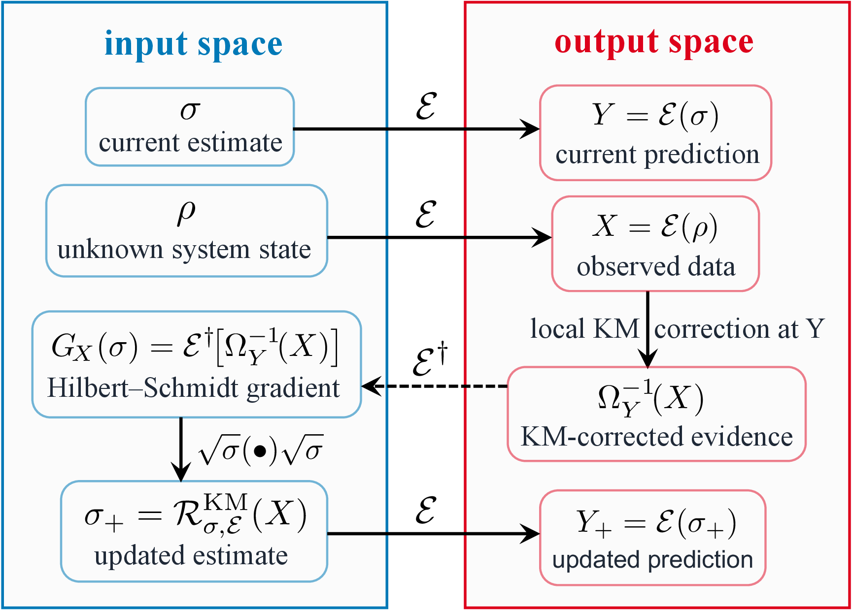representation of the KM update. The current estimate \(\sigma\) predicts \(Y=\mathcalE(\sigma)\), while the data define an output-space evidence operator \(X\); ideally, \(X=\mathcalE(\rho)\). The inverse KM action at \(Y\) gives the corrected evidence \(\Omega_Y^-1\!(X)\), which is pulled back through \(\mathcalE^\dagger\) to the Hilbert–Schmidt gradient \({G_{\!X}}(\sigma)\). Conjugation by \(\sqrt\sigma\) produces the positive state update \(\sigma_+=\mathcalR^\textKM_\sigma,\mathcalE(X)\), with updated prediction \(Y_+=\mathcalE(\sigma_+)\). :KM46update46schematic

Along with the Petz recovery map [57], the KM update is a possible generalization of Jeffrey’s rule to quantum physics. The above theorem and the previous conjecture imply that the application of this version of Jeffrey’s rule always increases the log-likelihood. This generalizes the classical result of Jacobs [94], see App. [sec:app:subsec:quantum46Bayes46theorem].

Note that replacing the KM update with the Petz recovery map in Conjecture 3 does not satisfy the desired inequality: since the Petz map is not the exact gradient of the log-likelihood 2 , applying it at a maximizer for noncommuting outputs with overcomplete basis and imperfect data can decrease it. A concrete example exhibiting a large violation is provided in App. [sec:app:subsec:quantum46Bayes46theorem].

KM update and Petz recovery as quantum tomography methods.

The following observation, which is a rephrasing of the discussion below Eq. 10 combined with concavity of the log-likelihood (see App. [sec:app:subsec:log46likelihood46concavity]), provides the basis for the KM update as a tomography method.

Theorem 2 guarantees that a line-search implementation can choose a step that increases the log-likelihood whenever the current state is not stationary. By Theorem 5, any full-rank fixed point reached by the iteration is a maximizer.

For the full step \(\eta = 1\) in the Petz case, we prove monotonicity and subsequential fixed-point convergence; under uniqueness of the relevant fixed point, the whole sequence converges. We conjecture that the analogous full-step statement extends to the KM update.

Using these results, we design a quantum tomography method as follows. Consider a set \(\{\mathcal{E}_j\}\) of channels with corresponding estimated outputs \(X_j\). Define the weighted log-likelihood as \[\require{physics} \sum\nolimits_j w_j \mathcal{L}_{X_j}(\sigma), \quad \mathcal{L}_{X_j}(\sigma) = \Tr\bigl[X_j \ln \mathcal{E}_j(\sigma)\bigr],\] which generalizes the standard maximum-likelihood formulation. The weights \(\{w_j\}\) represent the relative importance of each dataset and, in analogy with the usual log-likelihood, are typically chosen as empirical frequencies \(w_j = N_j / N\) of channel executions yielding data \(X_j\).

Due to the linearity of the Fréchet derivative, we can define the weighted KM update as \[\mathcal{R}^{\text{KM}}_{\sigma,\{\mathcal{E}_j\}}(\{X_j\}) \mathrel{\rlap{ \raisebox{0.3ex}{\m@th\cdot}} \raisebox{-0.3ex}{\m@th\cdot}} = \sum\nolimits_j w_j \mathcal{R}^{\text{KM}}_{\sigma,\mathcal{E}_j}(X_j), \label{def46weighted46KM46update}\tag{16}\] which corresponds to the gradient of the weighted log-likelihood in the inverse-square-root metric 7 . Equivalently, this is the ordinary KM update for the block channel \(\mathcal{E}_\oplus = \bigoplus_j w_j \mathcal{E}_j\) with data \(X_\oplus=\bigoplus_j w_j X_j\), up to an irrelevant additive constant in the likelihood, see App. [sec:app:subsec:block46channel]. This construction translates a tomography problem with several measurements into one with a single measurement and thus generalizes the theorems above.

The channel set may be undercomplete, overcomplete, or informationally complete. Quantum tomography is performed by iterating the KM update from an initial prior \({\sigma}_0\). Together with the prior, the weights determine the point in the null space (set of log-likelihood maximizers) to which the iteration converges or, for imperfect data, the boundary point it approaches, see Fig. [fig:convergence]. In the overcomplete case, the weights also encode the relative importance of different channels, prioritizing those with more reliable data.

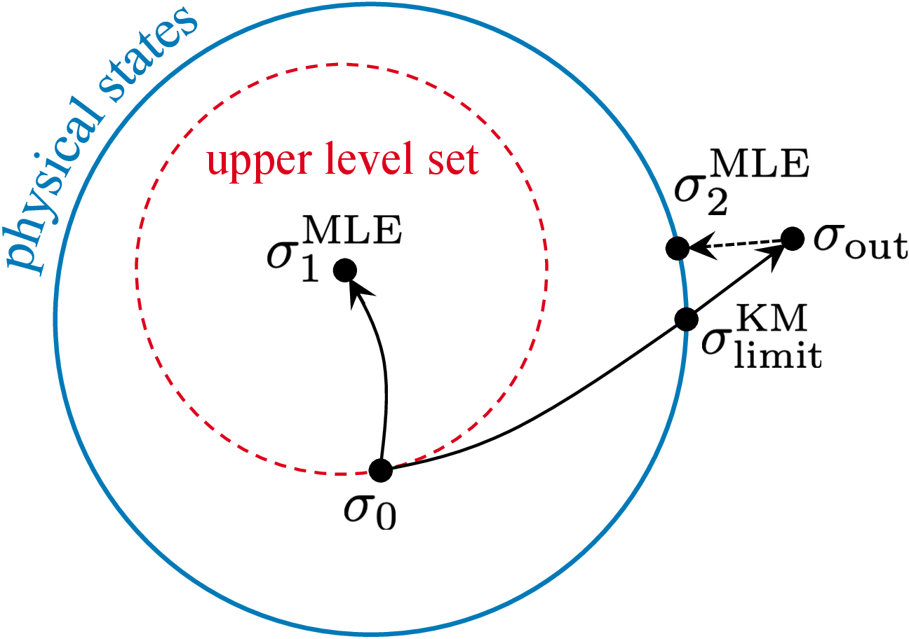
KM iteration converges locally to the maximum-likelihood estimator (MLE), provided the initial prior is sufficiently close. Otherwise, it may instead follow the log-likelihood gradient to a boundary point rather than the MLE, for example, when finite data make the observations incompatible with any physical state.

:convergence

We illustrate the method in Fig. [fig:petz50] on the standard tomography setup using Pauli measurements on six qubits and on the following noncommutative KM example: Defining a Stinespring channel, \(\mathcal{S}\mathrel{\rlap{ \raisebox{0.3ex}{\m@th\cdot}} \raisebox{-0.3ex}{\m@th\cdot}} =U(\bullet \otimes \ketbra{0}{0} )U^\dagger\), we denote system and environment marginals, and quantum-to-classical correlation channels, \[\require{physics} \begin{align} {\mathcal{E}}_S&=\Tr_E\mathcal{S}, \quad {\mathcal{E}}_E=\Tr_S\mathcal{S},\\ \mathcal{E}_C &= \bigoplus_{(a,b)} \tfrac{1}{9} \sum_{i,j} \Tr\!\left[ P_i^{(a)} \!\otimes\! P_j^{(b)}\mathcal{S}(\bullet) \right] \ketbra{ab,ij}{ab,ij}, \nonumber \end{align}\] where \(a\) and \(b\) represent different settings of Pauli measurements. We perform tomography by iterating the weighted KM update 16 using these highly overcomplete and incompatible channels. For the Petz map, we also consider a stabilized iteration, \({\sigma}_{k+1}=(1-\delta)({\sigma}_k)_+ +\delta I/d\), which improves convergence by preventing the state from approaching the boundary. For initial priors sufficiently close to the limit point, we observe that the tomography method converges exponentially fast.

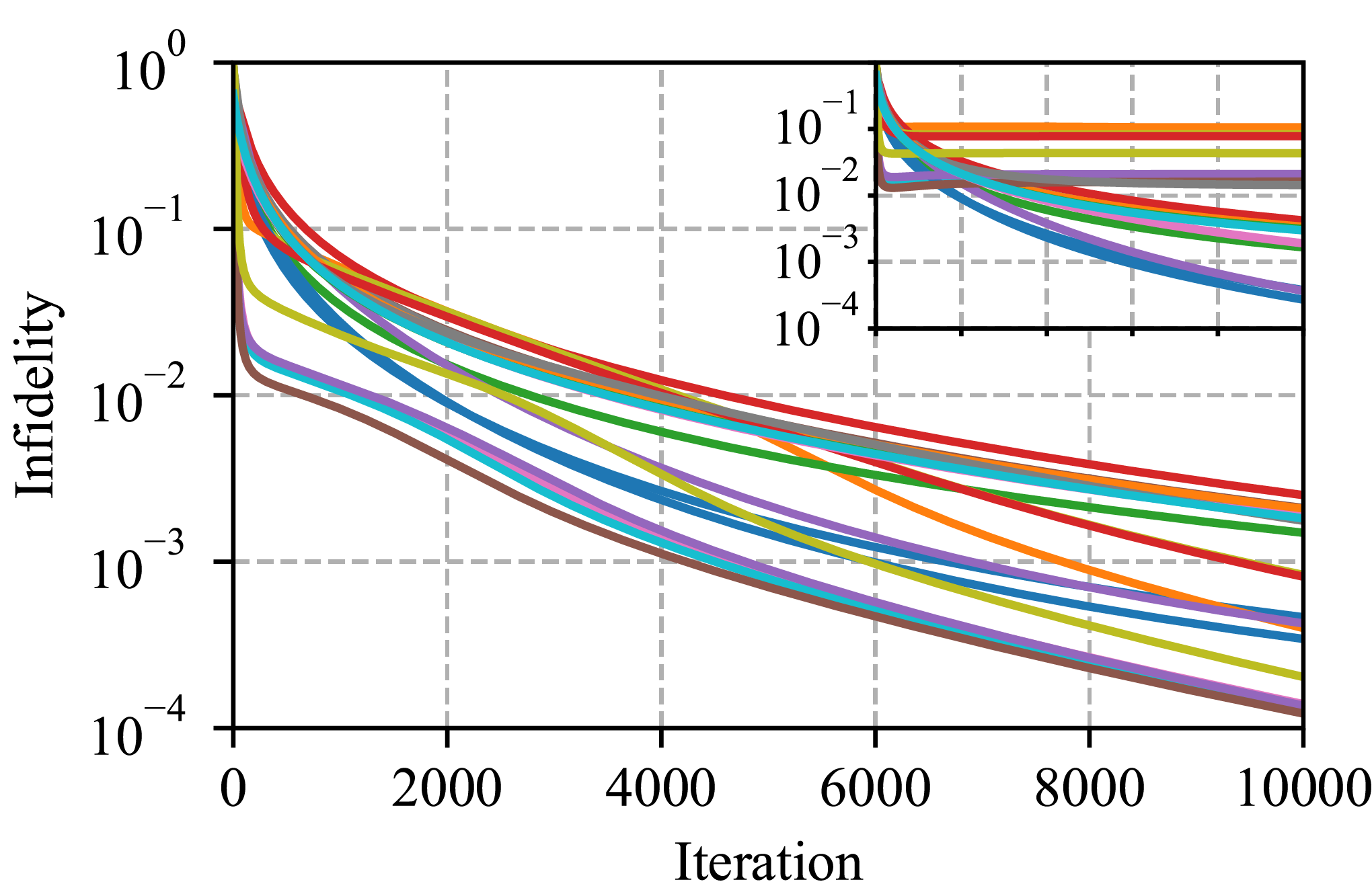
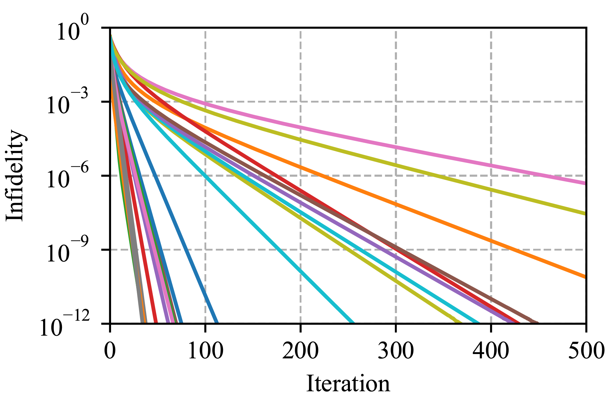: Maximum-likelihood quantum tomography based on iterative application of the weighted Petz map over Pauli bases, with the prior initialized as the maximally mixed state. Twenty states of six qubits of varying rank were randomly generated (including \(20\%\) pure states), and regularized to make them full-rank, \({\rho}=(1-\epsilon){\rho}+\epsilon I/d\), \(\epsilon = 10^-2\). We show the stabilized iteration (\(\delta=10^-7\)) and the unstabilized case (\(\delta=0\)) in the inset. Right: Tomography of a qubit via iterative unstabilized KM updates in a Stinespring setup with three overcomplete, incompatible channels defined by a random unitary U, using otherwise identical settings. The method converges faster for highly mixed states. The unstabilized iteration can exhibit premature numerical stagnation near the boundary, as shown in the inset. :petz50

2 Discussion and conclusions↩︎

In this paper, we studied the exact gradient of the log-likelihood functional and found that it leads to an update rule that we call the KB update. Together with the Petz recovery map and the rotated Petz recovery map, the KM update may be viewed as a candidate quantum analogue of Bayes’ and Jeffrey’s rule. All three maps reduce to the classical Bayes update in the commuting case. Unlike the Petz map, which arises naturally in the characterization of equality in the data-processing inequality [39], [41], or the rotated Petz map, which strengthens this connection through fidelity-based recovery bounds [46], [47], the KM update arises from the maximum-likelihood inference problem, namely the task of finding the reference state whose predicted output best explains the observed data.

More specifically, if closeness is quantified by the Umegaki quantum relative entropy (a choice supported by its uniqueness under four natural axioms [95]), then the KM update is its gradient with respect to the reference state and therefore follows the direction of steepest descent. Conjecture 3 and Theorem 4 further suggest that it monotonically decreases the relative entropy, extending Jacobs’ monotonicity result for Jeffrey’s rule and the Kullback–Leibler divergence [94]. In contrast, the Petz recovery map violates the analogous monotonicity property.

Since it is the unit natural-gradient step of the log-likelihood, the KM update has the structural features expected of a tomographic iteration, including the local monotonicity and convergence properties established in Theorems 2 and 5. In the commuting-output setting, the KM iteration reduces to the Petz iteration, for which we establish the stronger properties of full-step monotonicity and convergence to the maximum-likelihood estimator in Theorems 4 and 6.

This allows us to design and implement a tomographic protocol that is a first-order gradient-ascent method, applicable both to standard quantum tomography via the quantum-to-classical channel and to a multi-view reconstruction using general quantum channels. This is realized by formulating the weighted KM update 16 , which enables us to treat undercomplete, informationally complete, overcomplete, and imperfect data within a unified framework.

An interesting comparison can be made with Bayesian quantum tomography, which applies the classical Bayes theorem to infer a posterior distribution over quantum states. A common point estimate is the Bayesian mean estimator, \(\hat{\sigma}_{\text{BME}} = \int \sigma\, p(\sigma | \text{data})\, d\sigma,\) obtained by averaging over the posterior distribution [14]–[20]. In contrast to the present approach, this integral is generally not available in closed form and is typically approximated using methods such as sequential Monte Carlo or Metropolis–Hastings sampling [96].

Here, we find the KM update to generalize Bayes’ and Jeffrey’s rules, while being formulated entirely in terms of quantum states rather than probability distributions. Starting from the search for a fully quantum analogue of Bayesian inference, we therefore arrived at a somewhat surprising conclusion: the resulting update naturally leads to maximum-likelihood estimation. This raises the intriguing possibility that maximum-likelihood estimation is, in fact, the natural form of Bayesian inference in quantum theory.

The remaining open problems are to establish global monotonicity of the undamped KM update, derive general convergence guarantees, characterize its limiting points even in undercomplete settings, and develop faster and higher-order tomographic protocols inspired by the present approach.

Finally, the results presented here suggest that Kubo–Mori geometry provides the natural structure underlying maximum-likelihood estimation, thereby connecting quantum tomography, recovery maps, and quantum Bayesian retrodiction within a unified framework.

Acknowledgments↩︎

This research was supported by the Czech Science Foundation through the Junior Star grant 25-17250M (SM, FM, and DŠ) and by Charles University in Prague through PRIMUS/25/SCI/027 (IT and DŠ). We thank Joe Schindler and Valerio Scarani for the initial discussions that sparked this project, and especially Francesco Buscemi for early insights into the possible convergence of the Petz recovery map iteration.

Data availability↩︎

The source code used to generate Fig. [fig:petz50], the numerical evidence supporting Conjecture 3, and the search for the Petz monotonicity counterexample reported in the Appendix are available at https://github.com/dominik-safranek/km-update-tomography.

3 Supplementary Material↩︎

Contents

Let \(Y \!=\! \sum_i y_i\ketbra{i}{i}\), \(y_i \!>\! 0\). Then each matrix unit \(\ketbra{i}{j}\) is an eigenoperator of the modular generator \(K_Y \mathrel{\rlap{ \raisebox{0.3ex}{\m@th\cdot}} \raisebox{-0.3ex}{\m@th\cdot}} =[\ln Y,\cdot]\) with eigenvalue \[K_Y(\ketbra{i}{j}) = (\ln y_i-\ln y_j)\ketbra{i}{j} =\mathrel{\rlap{ \raisebox{0.3ex}{\m@th\cdot}} \raisebox{-0.3ex}{\m@th\cdot}}\omega_{ij}\ketbra{i}{j}.\] In the same basis, the inverse KM action is diagonal, \[\big(\Omega_Y^{-1}\!(X)\big)_{ij} = \frac{\ln y_i-\ln y_j}{y_i-y_j}\,X_{ij},\] with the diagonal case understood by continuity. Since \[y_i - y_j = 2\, \sqrt{y_i y_j}\, \sinh(\omega_{ij}/2),\] we obtain \[\big(\Omega_Y^{-1}\!(X)\big)_{ij} = k(\omega_{ij})\,\frac{X_{ij}}{\sqrt{y_i y_j}}, \quad k(\omega) = \frac{\omega}{2\sinh(\omega/2)}.\] Equivalently, \[\Omega_Y^{-1}\!(X) = k(K_Y)\!\big[Y^{-1/2}XY^{-1/2}\big].\] This proves the modular-frequency filter form in Theorem 1.

The same inverse KM action admits the integral representation \[\Omega_Y^{-1}\!(X) = \int_{\mathbb{R}} \beta_0(t)\, Y^{-(1+it)/2}X\,Y^{-(1-it)/2}\,dt, \label{eq:KM46integral46representation}\tag{17}\] where \(\beta_0(t) = \pi/[2(\cosh(\pi t)+1)]\) is normalized such that \[k(\omega) = \int_{\mathbb{R}} \beta_0(t)e^{-it\omega/2}\,dt.\] The same probability density \(\beta_0\) appears in Ref. [48] as the weight in the averaged rotated-Petz recovery map. Here, however, it represents the inverse KM operator itself rather than a CPTP average of recovery channels.

1. Linearity in \(\boldsymbol{X}\) \[\mathcal{R}^{\text{KM}}_{\sigma,\mathcal{E}}(aX_1+bX_2) = a\,\mathcal{R}^{\text{KM}}_{\sigma,\mathcal{E}}(X_1) + b\,\mathcal{R}^{\text{KM}}_{\sigma,\mathcal{E}}(X_2).\]

2. Positivity
   If \(X \geqslant 0\), then \[\mathcal{R}^{\text{KM}}_{\sigma,\mathcal{E}}(X) \geqslant 0,\] because \(\Omega^{-1}_Y\) is positive, \(\mathcal{E}^{\dagger}\) is positive, and conjugation by \(\sqrt{{\sigma}}\) preserves positivity.

3. Trace preservation in the argument \[\require{physics} \begin{align} \Tr\!\big[\mathcal{R}^{\text{KM}}_{\sigma,\mathcal{E}}(X)\big] &= \Tr\!\big[\sigma\, \mathcal{E}^{\dagger}[\Omega_Y^{-1}\!(X)]\big] =\Tr\!\big[\mathcal{E}(\sigma)\, \Omega_Y^{-1}\!(X)\big] \nonumber \\ &= \Tr\!\big[Y\, \Omega^{-1}_Y\!(X)\big] = \Tr[X]. \label{eq:KM46trace46preservation} \end{align}\tag{18}\] In particular, if \(X\) is a density operator, then \(\mathcal{R}^{\text{KM}}_{{\sigma},\mathcal{E}}(X)\) is again a density operator.

4. Exact recovery of the reference output \[\begin{align} \mathcal{R}^{\text{KM}}_{{\sigma},\mathcal{E}}\big(\mathcal{E}({\sigma})\big) = {\sigma}, \end{align}\] since \(\Omega^{-1}_Y(Y)=\mathbb{1}\) and \(\mathcal{E}^{\dagger}(\mathbb{1})=\mathbb{1}\).

5. Reduction to the Petz term in the commuting limit
   If \([X,Y]=0\), then \[\begin{align} \Omega^{-1}_Y\!(X)=Y^{-1/2} X Y^{-1/2}, \end{align}\] and therefore \[\begin{align} \mathcal{R}^{\text{KM}}_{{\sigma},\mathcal{E}}(X) = \sqrt{\sigma}\; \mathcal{E}^{\dagger}\!\big[ Y^{-1/2} X Y^{-1/2} \big]\, \sqrt{\sigma}, \end{align}\] which is the ordinary Petz recovery form.

6. Sum representation
   The KM update can be written as the sum \[\begin{align} \mathcal{R}^{\text{KM}}_{{\sigma},\mathcal{E}}(X) = {\sigma}+ \Delta^{\text{KM}}_{{\sigma},\mathcal{E}}(X), \end{align}\] with \(\Delta^{\text{KM}}_{{\sigma},\mathcal{E}}(X) \equiv G_{\!X}^\sigma(\sigma) - \sigma\), cf.Eqs. 12 and 14 .

7. Channel representation
   Introducing \[\begin{align} M_\sigma(A) &\mathrel{\rlap{ \raisebox{0.3ex}{\m@th\cdot}} \raisebox{-0.3ex}{\m@th\cdot}} =\mathcal{E} \big[\sqrt{\sigma}\,\mathcal{E}^\dagger(A)\,\sqrt{\sigma}\big], \\ \Phi_Y(A) &\mathrel{\rlap{ \raisebox{0.3ex}{\m@th\cdot}} \raisebox{-0.3ex}{\m@th\cdot}} =Y^{-1/2}\, M_\sigma(A)\; Y^{-1/2}, \end{align}\] the predicted output after the update \(Y_+ \mathrel{\rlap{ \raisebox{0.3ex}{\m@th\cdot}} \raisebox{-0.3ex}{\m@th\cdot}} =\mathcal{E}[\mathcal{R}^{\text{KM}}_{\sigma,\mathcal{E}}(X)]\) factorizes as \[Y_+ = M_{\sigma}[\Omega^{-1}_Y\!(X)] = \Phi_{Y,*}(\widehat{X}_Y),\] where \(\Phi_{Y,*}\) denotes the Hilbert–Schmidt adjoint of \(\Phi_{Y}\) and \(\widehat{X}_Y \mathrel{\rlap{ \raisebox{0.3ex}{\m@th\cdot}} \raisebox{-0.3ex}{\m@th\cdot}} =\sqrt{Y}\,\Omega^{-1}_Y\!(X) \sqrt{Y}\). Since \(\Phi_Y\) is unital CP, \(\Phi_{Y,*}\) is CPTP. Moreover, it preserves \(Y\), \(\Phi_{Y,*}(Y)=Y\). This is not the physical measurement channel itself, but an auxiliary CPTP map determined by \(Y\), \({\sigma}\), and \(\mathcal{E}\). The data processing inequality can be written in CPTP channel form as \[D (Y_+ \Vert Y) = D \big(\Phi_{Y,*}\big(\widehat{X}_Y\big) \big\Vert \Phi_{Y,*}(Y) \big) \leqslant D\big(\widehat{X}_Y \Vert Y\big).\]

For fixed \(X\geqslant0\), the map \[\require{physics} \sigma\mapsto \mathcal{L}_X(\sigma) = \Tr[X \ln \mathcal{E}(\sigma)]\] is concave on the domain where \(\mathcal{E}(\sigma)>0\). Indeed, for \(0\leqslant t\leqslant 1\), \[\require{physics} \begin{align} \mathcal{L}_X(t\sigma_1+(1-t)\sigma_0) &= \Tr\!\big[ X \ln\!\big(t \mathcal{E}(\sigma_1) + (1-t) \mathcal{E}(\sigma_0)\big) \big] \nonumber\\ & \geqslant t \mathcal{L}_X(\sigma_1) + (1-t) \mathcal{L}_X(\sigma_0), \end{align}\] by operator concavity of the logarithm and positivity of the trace pairing with \(X\). Consequently, for any two admissible states, \[\mathcal{L}_X(\rho) \leqslant \mathcal{L}_X(\sigma) + D\mathcal{L}_X(\sigma)[\rho-\sigma]. \label{eq:derivative95inequality}\tag{19}\]

In the quantum-to-classical case, write \(p_i \mathrel{\rlap{ \raisebox{0.3ex}{\m@th\cdot}} \raisebox{-0.3ex}{\m@th\cdot}} =\hat{p}_i\) and set \[\require{physics} \begin{align} \mathcal{S} &\mathrel{\rlap{ \raisebox{0.3ex}{\m@th\cdot}} \raisebox{-0.3ex}{\m@th\cdot}} =\{\sigma\geqslant0:\Tr[\sigma]=1\}, \\ \mathcal{D}_+ &\mathrel{\rlap{ \raisebox{0.3ex}{\m@th\cdot}} \raisebox{-0.3ex}{\m@th\cdot}} =\{\sigma\in\mathcal{S}:\Tr[\Pi_i\sigma]>0\;\;\forall\, i\}. \end{align}\] On states in \(\mathcal{S} \!\setminus\! \mathcal{D}_+\), the likelihood \(\mathcal{L}_{\text{qc}}\) is extended by setting \(\mathcal{L}_{\text{qc}}(\sigma)=-\infty\).

Lower bound.

Assume that \(Y>0\) and \(Y_\eta>0\), such that the logarithms below are ordinary matrix logarithms. We have \[\require{physics} \Tr[X \ln Y_\eta - X \ln Y]=D(X||Y)-D(X||Y_\eta),\] where \(Y=\mathcal{E}(\sigma)\) and \(Y_\eta=\mathcal{E}(\sigma_\eta)\). The quantum relative entropy, defined as [83], [86], \[\require{physics} \label{eq:quantum95relative95entropy} D(X||Y)=\Tr[X(\ln X-\ln Y)],\tag{20}\] can be expressed through the following optimization identity [97]: \[\require{physics} D(X||Y) = \sup_{H=H^\dagger} \big\lbrace \! \Tr[XH] - \ln \Tr\big[e^{H+\ln Y}\big] \big\rbrace.\] This implies \[\require{physics} \begin{align} \Tr[X \ln Y_\eta - X \ln Y] &= \sup_{H=H^\dagger} \big\lbrace \! \Tr[XH] - \ln \Tr[e^{H+ \ln Y}] \big\rbrace \nonumber \\ &- \sup_{\tilde{H} = \tilde{H}^\dagger} \big\lbrace \! \Tr\!\big[X \tilde{H}\big] - \ln \Tr\!\big[e^{\tilde{H} + \ln Y_\eta}\big] \big\rbrace \nonumber \\ &\geqslant -\ln \Tr[e^{\ln X - \ln Y_\eta + \ln Y}] + \ln \Tr[e^{\ln X}] \nonumber \\ &= - \ln \Tr[e^{\ln X - \ln Y_\eta + \ln Y}], \end{align}\] where we picked \(H = \tilde{H} = \ln X-\ln Y_\eta\), which maximizes the second supremum and gives a lower bound on the first.

We use Lieb’s triple-matrix inequality [97], [98]: for any positive definite operators \(R,S,T>0\), \[\require{physics} \Tr\!\left[e^{\ln R-\ln S+\ln T}\right] \leqslant \Tr\!\left[ R\,\Omega_S^{-1}\!(T) \right],\] where \[\Omega_S^{-1}\!(T) = \int_0^\infty (S+u\mathbb{1})^{-1}\,T\,(S+u\mathbb{1})^{-1} \,du .\] Using the theorem, we thus have \[\require{physics} \Tr[X \ln Y_\eta - X \ln Y] \geqslant - \ln \Tr[ X\, \Omega_{Y_\eta}^{-1}\!(Y)].\] Next, we derive, \[\require{physics} \begin{align} & 1 - \Tr[X\, \Omega_{Y_\eta}^{-1}\!(Y)] \nonumber \\ & = \Tr[\mathcal{E}^\dagger \big(\Omega_{Y_\eta}^{-1}\!(X)\big)(\sigma_\eta-\sigma)] \\ & = \eta \Tr[\big[\mathcal{E}^\dagger \big(\Omega_{Y_\eta}^{-1}\!(X)\big) - \mathbb{1}\big](\sigma_+ - \sigma)] \nonumber \\ & = \eta \Tr[\big[ \mathcal{E}^\dagger\!\big(\Omega_{Y_\eta}^{-1}\!(X)\big)-\mathbb{1}\big] \big(\sqrt{\sigma}\, \mathcal{E}^{\dagger} \!\big(\Omega_{Y}^{-1}\!(X)\big) \sqrt{\sigma} - \sigma \big)] \nonumber \\ &=\eta \textsl{g}_{\sigma} \Big( \sqrt{\sigma}\big[ \mathcal{E}^\dagger\!\big(\Omega_{Y_\eta}^{-1}\!(X)\big) - \mathbb{1} \big] \sqrt{\sigma} , \sqrt{\sigma} \big[ \mathcal{E}^\dagger\!\big(\Omega_{Y}^{-1}\!(X)\big)-\mathbb{1} \big] \sqrt{\sigma} \Big) \nonumber \\ &= \eta \textsl{g}_{\sigma}(\Delta_{\sigma_\eta}^\sigma,\Delta_{\sigma}^\sigma). \nonumber \end{align}\] This provides the desired inequality, \[\require{physics}\Tr[X \ln Y_\eta - X \ln Y] \geqslant -\ln\!\big[1-\eta\,\textsl{g}_{\sigma}(\Delta_{\sigma_\eta}^\sigma,\Delta)\big],\] where we have set \(\Delta \equiv \Delta_{\sigma}^\sigma\).

Using the inequality \(-\ln(1-x)\geqslant x\), valid whenever \(x<1\), gives the looser inequality \[\require{physics} \Tr[X \ln Y_\eta \!-\! X \ln Y] \geqslant 1 \!-\! \Tr\big[X\, \Omega_{Y_\eta}^{-1}\!(Y)\big]\!=\!\eta \textsl{g}_{\sigma}(\Delta_{\sigma_\eta}^\sigma,\Delta).\] This can be independently derived using concavity of the log-likelihood 19 , and extends the inequality to semidefinite \(X\) for which the explicit optimizer \(H=\ln X-\ln Y_\eta\) has to be interpreted by approximation.

Upper bound.

Using Eq. 19 , we have \[\require{physics} \begin{align} \mathcal{L}_X(\sigma_\eta) - \mathcal{L}_X(\sigma) & \leqslant D\mathcal{L}_X(\sigma)[\sigma_\eta-\sigma] \\ &= \eta\,\Tr\!\left[\mathcal{E}^{\dagger}\!\big(\Omega_Y^{-1}\!(X)\big)\,\Delta\right] \nonumber \\ &= \eta\,\Tr\!\left[\left(\mathcal{E}^{\dagger}\!\big(\Omega_Y^{-1}\!(X)\big) - \mathbb{1}\right) \Delta\right] \nonumber \\ &= \eta\,\textsl{g}_{\sigma}(\Delta,\Delta), \nonumber \end{align}\] where \(Y=\mathcal{E}(\sigma)\) and \(\Delta=\sigma_+-\sigma=(\sigma_\eta-\sigma)/\eta\).

We will prove that every full-rank fixed point \(\sigma\) of the KM update is a maximizer of the log-likelihood. Since \(\sigma\) is full rank, the fixed-point equation \(\mathcal{R}^{\text{KM}}_{\sigma,\mathcal{E}}(X)=\sigma\) is equivalent to \({G_{\!X}}(\sigma)=\mathbb{1}\). Conversely, stationarity on the trace-one manifold gives \({G_{\!X}}(\sigma)=\lambda\mathbb{1}\), and taking the trace against \(\sigma\) gives \(\require{physics} \lambda=\Tr[X]=1\). Thus being a full-rank fixed point is equivalent to being a stationary point of the log-likelihood. In other words, as we have shown in the main text, the following statements are equivalent, \[\require{physics} \begin{align} \begin{aligned} D\mathcal{L}_X(\sigma)[\Delta']=0 \quad \forall\; \Delta'=\Delta'^\dagger,\; \Tr[\Delta']=0\\ \Longleftrightarrow\, {G_{\!X}}(\sigma)=\mathbb{1} \,\Longleftrightarrow\, \Delta=0 \,\Longleftrightarrow\, \mathcal{R}^{\text{KM}}_{\sigma,\mathcal{E}}(X)=\sigma. \end{aligned} \end{align}\] This follows from Eqs. 12 and 14 . Using concavity of the log-likelihood 19 , for any other state \(\sigma'\), we have \[\mathcal{L}_X(\sigma') \leqslant \mathcal{L}_X(\sigma) + D\mathcal{L}_X(\sigma)[\sigma'-\sigma] = \mathcal{L}_X(\sigma),\] where we selected \(\Delta'=\sigma'-\sigma\) for the first stationarity condition. Thus, the log-likelihood of any other state is upper-bounded by that at the stationary point; hence every full-rank stationary point is a maximizer of the log-likelihood.

In what follows, we use \(p_i \!\mathrel{\rlap{ \raisebox{0.3ex}{\m@th\cdot}} \raisebox{-0.3ex}{\m@th\cdot}} =\! \hat{p}_i \!\geqslant\! 0\) with \(\sum_i p_i \!=\! 1\), \(\require{physics} q_i \!\mathrel{\rlap{ \raisebox{0.3ex}{\m@th\cdot}} \raisebox{-0.3ex}{\m@th\cdot}} =\! \Tr[\Pi_i\sigma]>0\), \(\require{physics} q_i'\mathrel{\rlap{ \raisebox{0.3ex}{\m@th\cdot}} \raisebox{-0.3ex}{\m@th\cdot}} =\Tr[\Pi_i\sigma_+]\), and \(\| \!\cdot\!\|\) to denote the Hilbert–Schmidt norm. Terms with \(p_i=0\) are understood as omitted in expressions containing \((Cp)_i\) or \(q_i'\) in a denominator, or containing \(q_i'\) inside a logarithm or inside \(f(q_i'/q_i)\). Let \[p = \begin{pmatrix} p_1 \\ \vdots \\ p_m \end{pmatrix},\quad q = \begin{pmatrix} q_1 \\ \vdots \\ q_m \end{pmatrix},\quad Q = \begin{pmatrix} q_1 & & 0 \\ & \ddots & \\ 0 & & q_m \end{pmatrix}.\] Next, define the \(m \!\times\! m\) positive semidefinite matrix \(B\) by \[\require{physics} B_{ij} \mathrel{\rlap{ \raisebox{0.3ex}{\m@th\cdot}} \raisebox{-0.3ex}{\m@th\cdot}} =\frac{1}{q_i q_j}\Tr[\Pi_i\sqrt{\sigma}\, \Pi_j\sqrt{\sigma}]. \label{def:Gram46matrix}\tag{21}\] The above is a Gram matrix: its entries are given by \(B_{ij} = \langle \frac{1}{q_i}\Pi_i,\frac{1}{q_j}\Pi_j\rangle_\sigma\), where \[\require{physics} \langle A,B\rangle_\sigma \mathrel{\rlap{ \raisebox{0.3ex}{\m@th\cdot}} \raisebox{-0.3ex}{\m@th\cdot}} =\Tr[A^\dagger \sqrt{\sigma}\, B \sqrt{\sigma}]\] is a positive semidefinite sesquilinear form on \(\mathbb{C}^{d\times d}\). When \(\sigma\) is full rank, it is an inner product, known as the KMS inner product [99]. We also let \(C=QB\). Thus, the entries of \(C\) are given by \[\require{physics} C_{ij} = \frac{1}{q_j} \Tr[\Pi_i\sqrt{\sigma}\, \Pi_j\sqrt{\sigma}].\] These entries are nonnegative, since \[\require{physics} \Tr[\Pi_i \sqrt{\sigma}\,\Pi_j\sqrt{\sigma}] = \left\|\Pi_i^{1/2}\sqrt{\sigma}\; \Pi_j^{1/2}\right\|^2 \geqslant 0 .\] Note that \(Cq=q\), since \[\require{physics} \begin{align} \begin{aligned} (Cq)_i & =\sum_j C_{ij}\, q_j =\sum_j \frac{1}{q_j}\Tr(\Pi_i\sqrt{\sigma}\, \Pi_j\sqrt{\sigma})q_j \\ &=\Tr\Big[\Pi_i\sqrt{\sigma}\, \sum_j\Pi_j\sqrt{\sigma}\Big] =\Tr[\Pi_i\sigma] = q_i. \end{aligned} \end{align}\] Finally, the spectral radius \(\rho(A)\) of a square matrix \(A\) is defined as \[\rho(A) = \max\{|\lambda|:\text{\lambda is an eigenvalue of A}\}.\]

It remains to prove monotonicity and the equality condition; this is the content of Theorem 7 below, whose proof uses Lemma 7.

Together with the explicit formula for the Petz update established above, this proves Theorem 4.

Note that this theorem extends to any number of measurements by the construction from App. [sec:app:subsec:block46channel].

We assumed that all observed probabilities \(p_i^j\) are positive. In quantum state tomography, this can be ensured by additive smoothing \[\hat{p}_i=\frac{N_i+\alpha}{N+\alpha m},\] where \(N_i\) is the number of times outcome \(i\) is observed, \(N\) is the total number of measurements, \(m\) is the number of possible measurement outcomes, and \(\alpha>0\) is a smoothing parameter.

A weighted likelihood for several channels can be written as a single-channel likelihood on a direct-sum output space. Define \[\mathcal{E}_{\oplus}(\sigma) = \bigoplus_j w_j\,\mathcal{E}_j(\sigma), \quad X_{\oplus} = \bigoplus_j w_j\,X_j, \quad \sum_j w_j = 1,\] and \(w_j\geqslant 0\). Then, up to the constant \(\require{physics} \sum_j w_j \Tr[X_j]\ln w_j\), \[\require{physics} \Tr[X_{\oplus}\ln\mathcal{E}_{\oplus}(\sigma)] = \sum_j w_j \Tr[X_j\ln\mathcal{E}_j(\sigma)].\] Moreover, since \(\Omega^{-1}_{w_jY_j}(w_jX_j)=\Omega^{-1}_{Y_j}(X_j)\), the KM update for \(\mathcal{E}_{\oplus}\) is exactly \[\mathcal{R}^{\text{KM}}_{\sigma,\mathcal{E}_{\oplus}}(X_{\oplus}) = \sum_j w_j\,\mathcal{R}^{\text{KM}}_{\sigma,\mathcal{E}_j}(X_j).\]

Example: quantum-to-classical channel.

For \(\require{physics} \mathcal{E}_j(\sigma) = \sum_i \Tr \big[\Pi_i^{(j)}\sigma\big] \ketbra{j,i}{j,i}\), the block channel \(\mathcal{E}_{\oplus}\) is the quantum-to-classical channel associated with the single POVM \(\{w_j\Pi_i^{(j)}\}_{i,j}\) and the block data \[X_{\oplus} = \sum_{j,i} w_j\hat{p}_i^{(j)} \ketbra{j,i}{j,i}.\] Thus the weighted Petz update is the ordinary Petz update for this unified POVM, and the weighted KM identity above reduces to the same construction in the commuting case.

Let \(X\) and \(Y\) be random variables taking values from finite sets \(\mathcal{X}\) and \(\mathcal{Y}\) respectively. We view the random variable \(X\) as representing the state of a classical system, while \(Y\) is the result of an observation on the system. The observation can be modeled as a “forward” process \(\mathcal{E}\) corresponding to the stochastic matrix with entries given by the conditional probabilities \(p(y|x)\) for \(x \!\in\! \mathcal{X}\) and \(y \!\in\! \mathcal{Y}\). Given a prior distribution \(\sigma(x)\) representing an agent’s belief about \(X\), we apply the forwards process to obtain the distribution \[\mathcal{E}(\sigma)(y) = \sum_{x\in\mathcal{X}} p(y|x)\, \sigma(x).\] If an observation \(y\) is made, Bayes’ rule prescribes the following update to the prior: \[\label{eq:bayes} \sigma_y(x) = \frac{p(y|x)\, \sigma(x)}{\sum_{x\in\mathcal{X}}\, p(y|x)\, \sigma(x)}.\tag{23}\] Jeffrey’s rule extends Bayes’ to situations with “soft evidence”, where the observation is a distribution \(\tau(y)\). In this case, the updated state is \[\sigma_+(x) = \sum_{y\in\mathcal{Y}} \sigma_y(x)\, \tau(y). \label{eq:jeffrey}\tag{24}\] The expression above has the form \(\sigma_+=\mathcal{R}_{\sigma,\mathcal{E}}(\tau)\), where \(\mathcal{R}_{\sigma,\mathcal{E}}\) is the Bayesian reverse process determined by the prior \(\sigma\) and the forward channel \(\mathcal{E}\). Bayes’ rule 23 is recovered when \(\tau\) is a delta distribution. Jeffrey’s rule follows from Jeffrey’s probability kinematics [100], is equivalent to Pearl’s virtual-evidence update [101], [102], and can also be derived from a minimum-change principle [57].

Viewing quantum mechanics as the noncommutative generalization of classical probability theory, one naturally asks for a quantum Bayes rule: a CPTP map \(\mathcal{R}\) extending 24 to quantum states and channels. Several inequivalent proposals exist [51], [52], [57], [103], reflecting the fact that no single quantum extension has the same universal status as classical Bayes’ rule. In the relative-entropy setting, the canonical object is the Petz recovery map 15 , which characterizes equality in the data-processing inequality [39]–[41] \[D(\mathcal{E}(\rho)\|\mathcal{E}(\sigma)) \leqslant D(\rho\|\sigma). \label{eq:data46processing46inequality}\tag{25}\] For faithful \(\sigma\) and compatible supports, equality holds precisely when \(\rho\) is recovered from its channel output by the Petz map, \(\mathcal{R}_{\sigma,\mathcal{E}}(\mathcal{E}(\rho))=\rho\).

Jacobs [94] showed that Jeffrey’s update moves the predicted observation toward the soft evidence in a precise relative-entropy sense: for the Kullback–Leibler divergence [104] \[D_{\text{KL}}(p\|q) \mathrel{\rlap{ \raisebox{0.3ex}{\m@th\cdot}} \raisebox{-0.3ex}{\m@th\cdot}} =\sum_z p(z)[\ln p(z)-\ln q(z)],\] one has \[D_{\text{KL}}(\tau\|\mathcal{E}(\sigma_+)) \leqslant D_{\text{KL}}(\tau\|\mathcal{E}(\sigma)),\] where \(\tau\), \(\mathcal{E}(\sigma_+)\), and \(\mathcal{E}(\sigma)\) are classical distributions.

Theorem 4 in the main text generalizes the Petz–Jeffrey monotonicity statement for quantum-to-classical channels 3 , whose outputs are mutually commuting, even though their quantum inputs need not be. This Theorem can be rewritten as, \[D\!\left(X\,\middle\|\,\mathcal{E}_{\text{qc}}(\sigma_+)\right) \leqslant D\!\left(X\,\middle\|\,\mathcal{E}_{\text{qc}}(\sigma)\right),\] with equality iff \(\sigma_+=\sigma\), and where \(\sigma_+ = \mathcal{R}_{\sigma,\mathcal{E}_{\text{qc}}}(X)\).

However, as mentioned in the main text, the Petz recovery map does not satisfy such a monotonicity theorem in general. The obstruction is the noncommutative output differential: when \([\mathcal{E}(\sigma),X]\neq0\), one generally has \[\Omega_{\mathcal{E}(\sigma)}^{-1}\!(X) \neq \mathcal{E}(\sigma)^{-1/2}X\,\mathcal{E}(\sigma)^{-1/2}.\] A concrete example which exhibits violation of this inequality is \[\begin{align} \sigma &= \begin{pmatrix} \frac{2}{3} & 0 \\ 0 & \frac{1}{3} \end{pmatrix}\!,\; X = \begin{pmatrix} 0.99 & 0 \\ 0 & 0.01 \end{pmatrix}\!,\; \mathcal{E}(\sigma) = \sum_{j=1}^{2} K_j \sigma K_j^\dagger,\nonumber \\ K_1 &\!=\! \begin{pmatrix} -0.251899 \!+\! 0.447484\,i & \;\;0.284823 \!-\! 0.031868\,i \\ 0.308714 \!-\! 0.635360\,i & -0.388139 \!+\! 0.067281\,i \end{pmatrix}\!,\nonumber \\ K_2 &\!=\! \begin{pmatrix} -0.215046 \!+\! 0.189193\,i & -0.500736 \!-\! 0.114805\,i \\ 0.279643 \!-\! 0.277632\,i & 0.696647 \!+\! 0.115962\,i \end{pmatrix}\!. \end{align}\] For the Petz recovery map \(\mathcal{R}_{\sigma,\mathcal{E}}\), we obtain \[D\!\left(X\,\middle\|\,\mathcal{E}(\sigma)\right)-D\!\left(X\,\middle\|\,\mathcal{E}(\mathcal{R}_{\sigma,\mathcal{E}}(X))\right)=-2.022036,\] while for the KM update \(\mathcal{R}^{\text{KM}}_{\sigma,\mathcal{E}}\), we have \[D\!\left(X\,\middle\|\,\mathcal{E}(\sigma)\right)-D\!\left(X\,\middle\|\,\mathcal{E}(\mathcal{R}^{\text{KM}}_{\sigma,\mathcal{E}}(X))\right)=0.069089.\] Notice that in this case \(X\) and \(Y=\mathcal{E}(\sigma)\) are highly non-commuting; the Frobenius norm is equal to \(\norm{[X,Y]}_F=0.659206\), which is close to the maximum given by \(1/\sqrt{2}\). This example was found numerically using random instances further refined by simulated annealing.

This is consistent with Theorem 1 of Ref. [57], where the Petz map is recovered as the solution of the minimum-change problem in the output-commuting case \([\mathcal{E}(\sigma),X]=0\). The corresponding noncommutative likelihood-gradient correction is the inverse KM action derived in Sec. 1.

The quantum-to-classical channel is defined as \[\require{physics} {\mathcal{E}}_{\text{qc}}(\sigma) = \sum_i \Tr[\Pi_i \sigma] \ketbra{i}{i}. \label{app:eq:qc46channel}\tag{26}\] Using \(\Pi_i=K_i^\dagger K_i\), we can rewrite it in terms of its Kraus decomposition as \[{\mathcal{E}}_{\text{qc}}(\sigma) = \sum_{i,j} \ketbra{i}{j} K_i \sigma K_i^\dagger\ketbra{j}{i},\] with adjoint \[{\mathcal{E}}_{\text{qc}}^\dagger(Z) = \sum_{i,j} K_i^\dagger\ketbra{j}{i} Z \ketbra{i}{j} K_i.\]

The inverse KM superoperator is \[\Omega_{{\mathcal{E}}_{\text{qc}}(\sigma)}^{-1}\!(X) = \int_{\mathbb{R}} \beta_0(t)\, {\mathcal{E}}_{\text{qc}}(\sigma)^{-(1+it)/2}X\,{\mathcal{E}}_{\text{qc}}(\sigma)^{-(1-it)/2}\,dt.\] If \(X\) is diagonal in the \(\{\ket{i}\}\) basis, e.g., because it has been produced by the quantum-to-classical channel, then \(X=\sum_i \hat{p}_i\ketbra{i}{i}\), \({\mathcal{E}}_{\text{qc}}(\sigma)\) and \(X\) commute, and \[\require{physics} \Omega_{{\mathcal{E}}_{\text{qc}}(\sigma)}^{-1}\!(X) = {\mathcal{E}}_{\text{qc}}(\sigma)^{-1/2}X\,{\mathcal{E}}_{\text{qc}}(\sigma)^{-1/2}=\sum_i \frac{\hat{p}_i}{ \Tr[\Pi_i \sigma]}\ketbra{i}{i}.\] This means that the Hilbert-Schmidt gradient is \[\require{physics} \begin{align} {G_{\!X}}(\sigma) &= \mathcal{E}^{\dagger}\!\big[\Omega_{{\mathcal{E}}_{\text{qc}}(\sigma)}^{-1}\!(X)\big] = \sum_{i,j} K_i^\dagger\ket{j} \frac{\hat{p}_i}{ \Tr[\Pi_i \sigma]} \bra{j} K_i \nonumber \\ &= \sum_{i} \frac{\hat{p}_i}{ \Tr[\Pi_i \sigma]} \Pi_i, \end{align}\] and the gradient in the inverse square-root metric 7 is \[\require{physics} G_{\!X}^\sigma(\sigma)= \sqrt{\sigma}\, {G_{\!X}}(\sigma) \sqrt{\sigma}=\sum_{i} \frac{\hat{p}_i}{ \Tr[\Pi_i \sigma]} \sqrt{\sigma}\, \Pi_i \sqrt{\sigma}.\] This leads to the Riemmanian gradient, \[\require{physics} \Delta = G_{\!X}^\sigma(\sigma)-\sigma = \sqrt{\sigma}\Big(\sum_{i} \frac{\hat{p}_i}{ \Tr[\Pi_i \sigma]} \Pi_i - I \Big) \sqrt{\sigma}.\]

If \(X={\mathcal{E}}_{\text{qc}}(\rho)\) has been computed directly as an output of the channel for a state \(\rho\), then \(\require{physics} \hat{p}_i\equiv p_i=\Tr[\Pi_i\rho]\), and the KM update applied to \({\mathcal{E}}_{\text{qc}}(\rho)\) equals the Petz recovery map, \[\require{physics} \mathcal{R}^{\text{KM}}_{\sigma,{\mathcal{E}}_{\text{qc}}}({\mathcal{E}}_{\text{qc}}(\rho)) = \mathcal{R}_{\sigma,{\mathcal{E}}_{\text{qc}}}({\mathcal{E}}_{\text{qc}}(\rho)) = \sum_{i} \frac{p_i}{\Tr[\Pi_i \sigma]} \sqrt{\sigma}\, \Pi_i \sqrt{\sigma}.\]

Inserting the quantum-to-classical channel and \(X\) into the generalized log-likelihood, we obtain \[\require{physics} \begin{align} \mathcal{L}_X(\sigma) &= \Tr\!\big[X \ln {\mathcal{E}}_{\text{qc}}(\sigma)\big] \\ &= \Tr\!\bigg[\sum_i \hat{p}_i\ketbra{i}{i} \ln \Big(\sum_i \Tr[\Pi_i \sigma] \ketbra{i}{i}\Big)\bigg] \\ &=\sum_i \hat{p}_i \ln \Tr[\Pi_i \sigma]. \end{align}\] This is the standard log-likelihood.

For a line search update \[\sigma_\eta = \sigma + \eta\, \Delta, \qquad f(\eta) \mathrel{\rlap{ \raisebox{0.3ex}{\m@th\cdot}} \raisebox{-0.3ex}{\m@th\cdot}} =\mathcal{L}_X(\sigma_\eta),\] the quantum-to-classical channel gives \[\require{physics} \begin{align} \begin{aligned} f'(0) &= \textsl{g}_\sigma(\Delta,\Delta) = \|\Delta\|_{\textsl{g}_\sigma}^2\\ &=\Tr[\left(\bigg(\sum_{i} \frac{\hat{p}_i}{ \Tr[\Pi_i \sigma]} \Pi_i - I \bigg)\sqrt{\sigma}\right)^2] . \end{aligned} \end{align}\] This means an approximate increase in the log-likelihood when performing a line search update, \[\mathcal{L}_X(\sigma_\eta)\approx \mathcal{L}_X(\sigma) + \eta\, f'(0).\]

References↩︎

---

1. Equivalently, if \(f(A) \mathrel{\rlap{ \raisebox{0.3ex}{\m@th\cdot}} \raisebox{-0.3ex}{\m@th\cdot}} =\ln A\), then the Fréchet derivative of \(f\) at \(Y\) is the linear map \(D f(Y) =\mathrel{\rlap{ \raisebox{0.3ex}{\m@th\cdot}} \raisebox{-0.3ex}{\m@th\cdot}}\Omega^{-1}_Y\), i.e., \(Df(Y)[X]=\Omega^{-1}_Y\!(X)\) [92].↩︎