: an Open-Source Python Package for Simulating Axion-Induced Spin Dynamics
January 01, 1970
Abstract
The interaction of ultralight bosonic dark matter with spins can be interpreted as a pseudomagnetic field acting on normal matter. Such interactions can be modeled as usual magnetic interactions using spin-evolution (Bloch) equations. , an open-source Python package for simulating spin dynamics induced by both usual and exotic interactions, is presented. The numerical simulations serve as a tool for deriving axion signal signatures, which are crucial for designing experimental searches and data analysis. Simulations are calibrated against theoretical expectations, ensuring the accuracy of the simulated signals. is available at https://github.com/Yuzhe98/AxionBloch, allowing researchers to simulate pseudomagnetic signals under specific configurations of the axion models and experimental setups. The package is documented at http://axionbloch.readthedocs.io/ and includes example scripts for application.
1 Introduction↩︎
The axion was originally proposed to resolve the strong \(CP\) problem in quantum chromodynamics [1]–[4]. Here \(C\) denotes charge conjugation and \(P\) denotes parity. Later, more general axionlike particles (ALPs) were proposed in various extensions of the Standard Model associated with spontaneously broken global symmetries [5]–[8]. Concerning the cosmological implications, axions and ALPs are also well-motivated dark matter candidates [9]–[11]. In this paper, axions and ALPs are referred to as “axions” for simplicity.
Axions may possess couplings to ordinary Standard Model particles [12], including photons, gluons, and fermions. Crucially, axion field gradients (\(\mathbf{\nabla}a\)) may couple to fermionic spins through a pseudoscalar interaction. The Hamiltonian for this interaction can be expressed as \[\mathcal{H}_{\mathrm{int}} = - g_\mathrm{aNN} \mathbf{\nabla}a \cdot \mathbf{S}\,,\] where \(g_\mathrm{aNN}\) is the axion-spin coupling strength, and \(\mathbf{S}\) is the spin operator. The axion field gradient can be regarded as a pseudomagnetic field that mimics the behavior of a real magnetic field, where the Hamiltonian can be written as \[\mathcal{H} = -\hbar \gamma \mathbf{B} \cdot \mathbf{S} \,,\] where \(\gamma\) is the gyromagnetic ratio of the spin, and \(\mathbf{B}\) is the magnetic field. The pseudomagnetic field induces spin dynamics, providing a pathway for detection in precision measurement experiments such as nuclear magnetic resonance (NMR) and comagnetometer-based searches [13]–[36]. There have been dedicated studies of the axion-induced spin dynamics [37]–[39], providing axion signal signatures and experimental sensitivity to axion fields. However, to our knowledge, there have not been studies taking advantage of numerical methods to verify the derived axion signal signatures. On the other hand, as more axion models and experiments are being proposed, such as cosmic axion background [40], [41], fine-grained axion [42], and quadratically coupled axion [43], [44], a tool is needed to systematically simulate the axion-induced spin dynamics under various physical conditions and axion field configurations.
In this work, , an open-source package designed to simulate spin dynamics induced by axion fields, is introduced. The interface is implemented in Python, a programming language known for its simplicity and readability, while the underlying numerical integration is implemented in C++ for efficiency. The package provides a flexible framework for modeling axion fields and experimental configurations. By numerically solving spin-evolution equations, enables the prediction and analysis of experimentally observable signals.
2 Capabilities↩︎
In this section, the main components of are described. The section starts with the units, physical quantities, and constants (2.1). Then, it continues with the physics and the algorithm for the numerical simulation (2.2), after which the calibration for the simulation follows (2.3). In the end, an example simulation of axion-induced signals is provided (2.4).
2.1 Units, physical quantities, and constants↩︎
The package takes advantage of astropy1 [45] to
deal with units and physical quantities. Using astropy.units, physical quantities are created by attaching units to Python scalars or NumPy2 [46] arrays. Quantities can be converted between dimensionally equivalent units using the to() method. In astropy, unit
definitions are included in both the International System of Units (SI) and the Centimeter-Gram-Second (CGS) systems. Values in SI or CGS units can be found in the quantity’s properties .si and .cgs. A code example can be found in
1.
In axionbloch.constants, a few commonly-used constants in axion and NMR research, such as gyromagnetic ratios, are defined. The constants are instances of astropy.units.Quantity; therefore, all operations on physical quantities
are supported for the constants.

Figure 1: Examples of operations on physical quantities using astropy.units and axionbloch.constants..
2.2 Algorithm↩︎
2.2.1 Spin dynamics↩︎
Considering the current experiments looking for axion-induced spin dynamics, focuses on spin-\(1/2\) magnetic resonance. Different spins may be addressed in future updates. Magnetization is used as the observable to characterize the spin ensemble. In the presence of magnetic fields or axion-induced pseudomagnetic fields, the magnetization \(\mathbf{M}\) evolves as \[\begin{align} \frac{d M_x}{dt} &= \gamma \left( \mathbf{M} \times \mathbf{B}_{\mathrm{eff}} \right)_x - \frac{M_x}{T_2}\,,\tag{1} \\ \frac{d M_y}{dt} &= \gamma \left( \mathbf{M} \times \mathbf{B}_{\mathrm{eff}} \right)_y - \frac{M_y}{T_2}\,,\tag{2} \\ \frac{d M_z}{dt} &= \gamma \left( \mathbf{M} \times \mathbf{B}_{\mathrm{eff}} \right)_z - \frac{M_z - M_0}{T_1}\,,\tag{3} \end{align}\] where \(\gamma\) is the gyromagnetic ratio, \(\mathbf{B}_{\mathrm{eff}}\) is the total effective field, \(T_1\) and \(T_2\) are relaxation times, and the subscripts \(x\), \(y\), \(z\) denote the Cartesian components. The bias field is usually much stronger than the pseudomagnetic field. Therefore, the rotating coordinate frame (RCF) is adopted to remove the Larmor precession due to the bias field, allowing efficient simulation of the slower axion-induced dynamics of interest.
The transverse relaxation time, characterized by time constant \(T_2^*\), includes the \(T_2\) relaxation and the dephasing due to the inhomogeneity of the bias field. Such inhomogeneity
of the bias field is simulated by sampling the spread of the bias fields in the Magnet instance, and solving the Bloch equations for individual bias fields.
2.2.2 Numerical integration↩︎
To derive the time evolution of the magnetization, numerically integrates the Bloch equations using the fourth-order Runge–Kutta (RK4) method. Given a time step \(\Delta t\), an effective magnetic field, and initial magnetization \(\mathbf{M}^0\), the magnetization at the \((n+1)\)-th step can be found via \[\mathbf{M}^{n+1} = \mathbf{M}^n + \frac{\Delta t}{6} \left( \mathbf{k}_1 + 2\mathbf{k}_2 + 2\mathbf{k}_3 + \mathbf{k}_4 \right)\,.\] Here \[\begin{align} \mathbf{k}_1 &= \left.\frac{d\mathbf{M}}{dt}\right|_{\mathbf{M}=\mathbf{M}^n}\,, \\ \mathbf{k}_2 &= \left.\frac{d\mathbf{M}}{dt}\right|_{\mathbf{M}=\mathbf{M}^n + \frac{1}{2}\mathbf{k}_1\Delta t}\,, \\ \mathbf{k}_3 &= \left.\frac{d\mathbf{M}}{dt}\right|_{\mathbf{M}=\mathbf{M}^n + \frac{1}{2}\mathbf{k}_2\Delta t}\,, \\ \mathbf{k}_4 &= \left.\frac{d\mathbf{M}}{dt}\right|_{\mathbf{M}=\mathbf{M}^n + \mathbf{k}_3\Delta t}\,, \end{align}\] where \(d\mathbf{M}/dt\) can be found using the Bloch equations [Eqs. (1 –3 )]. This fourth-order method yields a local truncation error of \(\mathcal{O}(\Delta t^5)\), while the accumulated error over \(N = 1/\Delta t\) steps is of order \(\mathcal{O}(\Delta t^4)\). The time step \(\Delta t\) is usually set to be at least one order of magnitude smaller than the characteristic timescales of the system, such as relaxation times.
2.2.3 Implementation↩︎
Using object-oriented programming, the algorithm is implemented in a modular way to separate experimental configuration, axion field modeling, and numerical integration, allowing for flexible configuration of simulations. A diagram of the architecture of is shown in 2.
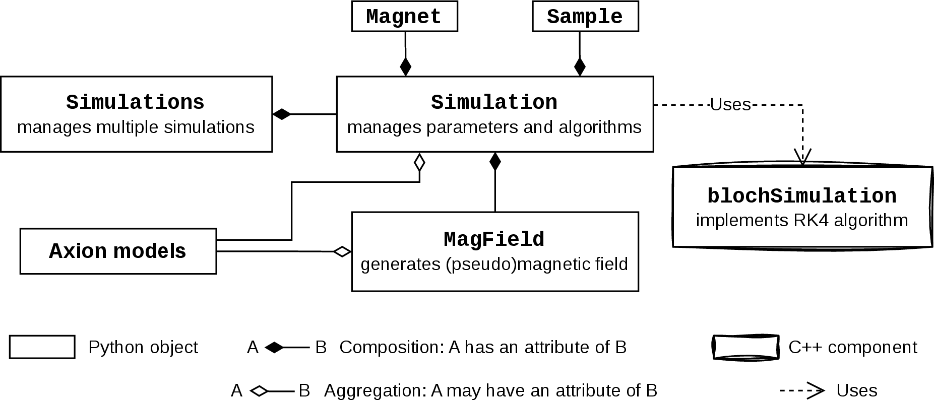
Figure 2: Architecture of . Each Simulation instance imports parameters from Magnet, Sample, and MagField instances. For axion simulations, axion-model objects are required both for
Simulation to configure the simulation and for MagField to generate the pseudomagnetic field. Simulations manages one or multiple Simulation instances. Numerical integration is performed via the
blochSimulation API, which provides Python access to the underlying C++ implementation..
On the Python side, classes Sample, Magnet, and MagField encapsulate the relevant experimental parameters, including sample relaxation times, magnetic field strength, and inhomogeneity. The axion models are
implemented by dedicated classes, such as MilkyWayAxionHalo, which carry the properties of the axion fields. Together with the method MagField.setAxionFields(), the pseudomagnetic fields can be generated. Different axion models
can be incorporated as separate classes without modifying the simulation framework. Simulation is handled within the axionbloch.SimuTools module. In particular, the classes Simulation and Simulations manage the
interaction between experimental configurations and axion models, organizing the parameters and execution of single or multiple simulation runs.
The RK4 algorithm is implemented in a dedicated C++ library. The application programming interface (API) for this library is blochSimulation. This C++ backend is interfaced with Python using pybind11,3 enabling cooperation between high-level Python workflow management and low-level efficient numerical computation.
2.3 Calibration↩︎
Accurate calibration is essential to ensure that the simulated signals reliably reflect the underlying physical system and can be compared with experimental observables. In particular, calibration examines the correspondence between the NMR signal and model parameters, including magnetic fields, nuclear spin gyromagnetic ratio \(\gamma\), and relaxation times (\(T_1\), \(T_2\), and \(T_2^*\)). It allows one to verify the correctness and stability of the numerical implementation. In this section, examples of calibration simulations are presented along with theoretical predictions, demonstrating the methodology of calibration. A quantitative analysis is included at the end of the section. For the examples in the section, an ethanol sample and an axial bias field \(\mathbf{B_{0}} = B_0 \mathbf{\hat{e}}_z\) are used.
2.3.1 Pulsed-NMR: free decay and spin echo↩︎
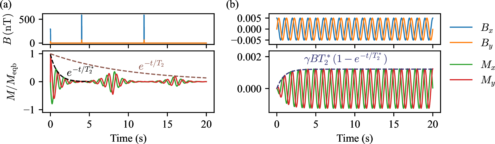
In the pulsed-NMR calibration, one \(\SI{90}{°}\) and one \(\SI{180}{°}\) magnetic-field pulse are applied in the simulation. The magnetization is expected to [47], [48]:
oscillate at the Larmor frequency;
be tipped by \(\SI{90}{°}\) to the x-y plane by the \(\SI{90}{°}\) pulse;
free decay with relaxation time \(T_2^*\) in the absence of pulses;
refocus (echo) after \(\SI{180}{°}\) pulses;
show decaying amplitude of echoes with relaxation time \(T_2\).
The behaviors described above can be found in the calibration example illustrated in 3 (a), indicating correct simulation behavior. With such a benchmark, magnetic pulses, Larmor precession, and transverse relaxations (\(T_2\) and \(T_2^*\)) can be calibrated.
2.3.2 Continuous-wave NMR↩︎
In the continuous-wave (CW) NMR calibration, an oscillating magnetic field is applied. When the magnetic field strength \(B\) is weak (\(\gamma B T_2^*\ll 1\)) and on resonance, the transverse magnetization grows with \(\gamma B T_2^* (1 - e^{-t/T_2^*})\) [48]. One such example is illustrated in 3 (b). The simulation produces the expected results. With such a benchmark, the Larmor precession and \(T_2^*\) relaxation can be calibrated.
2.3.3 Hyperpolarized sample↩︎
To achieve better sensitivity to the axion field, hyperpolarization is favored in experiments. Compared to thermal polarization at room temperature, hyperpolarization techniques can boost the polarization by orders of magnitude to the order of unity.
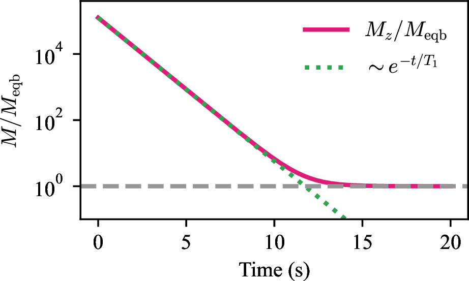
The package handles the polarization by the Sample class. A 1 %-polarization ethanol sample is used as an example demonstrating the evolution of polarization due to the \(T_1\) relaxation. At first (\(t\ll T_1\)), the polarization should exponentially decay with time constant \(T_1\), until it reaches equilibrium after many \(T_1\). As can be seen in 4, the simulated \(T_1\) relaxation agrees with the expected behavior. More of such simulations can be applied in calibrating \(T_1\) relaxation.
2.3.4 Quantitative evaluation↩︎
The accuracy of simulations is evaluated by the discrepancy between the theoretically expected magnetization and simulation results, characterized by \[\chi^2 = \dfrac{\sum |M_\mathrm{expected} - M_\mathrm{simu}|^2}{\sum |M_\mathrm{simu}|^2} \,. \label{eq:chisq}\tag{4}\] Here \(M_\mathrm{expected}\) and \(M_\mathrm{simu}\) are magnetization expected and simulated, respectively. \(\sum\) denotes the sum over integration steps. A well-calibrated simulation should give \(\chi^2\ll 1\). Calibration scripts are stored in the test suite of . In each calibration, parameters such as Larmor frequency and relaxation times are varied over orders of magnitude to cover all possible cases in simulation. The results of the calibrations are summarized in ¿tbl:tab:calibration95summary?. The discrepancies are generally small (\(\chi^2 < 10^{-4}\)). If a certain simulation precision is required, the \(\chi^2\) value serves as a quantitative reference.
| Calibration | Parameters calibrated | Varied parameters | \(\bm{\chi^2}\) | Dominant source of error |
|---|---|---|---|---|
| Pulsed NMR: free decay | Pulse amplitude, \(\nu_\mathrm{L}\), \(T_2^*\), \(T_2\) | \(\nu_\mathrm{RCF}\) | \(<10^{-4}\) | Finite number of steps for hard pulses. |
| CW-NMR | \(\nu_\mathrm{L}\) and \(T_2^*\) | \(\nu_\mathrm{RCF}\) | \(<10^{-5}\) | Finite integration step size. |
| \(T_1\) relaxation | \(T_1\) | \(\nu_\mathrm{RCF}\), \(\nu_\mathrm{L}\), initial polarization | \(<10^{-7}\) | Finite integration step size. |
2.4 Axion simulation↩︎
Similar to the calibration examples, axion-induced NMR signals are generated by solving the Bloch equations with the axion-induced pseudomagnetic field as part of the effective magnetic field. An example of a commonly considered model – axion
constituting the Milky Way galactic dark matter halo [49], [50] is implemented in the class MilkyWayAxionHalo. In this model, the axion field is treated as an oscillating field with a frequency determined by the axion mass,
and a linewidth (characterizing the stochasticity) determined by the velocity dispersion of the virialized dark matter halo. The sample is chosen to be , polarized to \(\SI{50}{\%}\) initially, and the bias field is applied
along the z direction. The details of the simulation configuration can be found in the code example in 5. Readers are referred to 2 which illustrates the relationship between the
objects in the code example. The simulated pseudomagnetic fields and the amplitude of the induced transverse magnetization are shown in 6, in which the signal increases with time at the beginning of the simulation
due to the pseudomagnetic field, and then decays due to the \(T_1\) relaxation. The efficiency of the simulation is limited by time consumption for the numerical integration of the Bloch equations. The total number of
integration steps \(N\) can be found by \[\begin{align} N &= \text{\texttt{Simulation.rate}} \times \text{\texttt{Simulation.duration}} \nonumber\\ &\quad \times
\text{\texttt{MagField.numFields}} \times \text{\texttt{Magnet.numPt}}\,,
\end{align}\] where Simulation.rate and Simulation.duration are the simulation rate and duration, MagField.numFields is the number of random pseudomagnetic fields generated to account for the stochasticity of
the axion field, and Magnet.numPt is the number of bias fields sampled to account for the inhomogeneity of the bias field. For the example in 5, the total number of integration steps is
7 × 10⁸, and the runtime is 2.7 s on a personal computer (CPU: Intel® Core Ultra 7 155H; base speed: 1.40 GHz). Such moderate runtime allows users to explore different parameter regimes with many simulations.
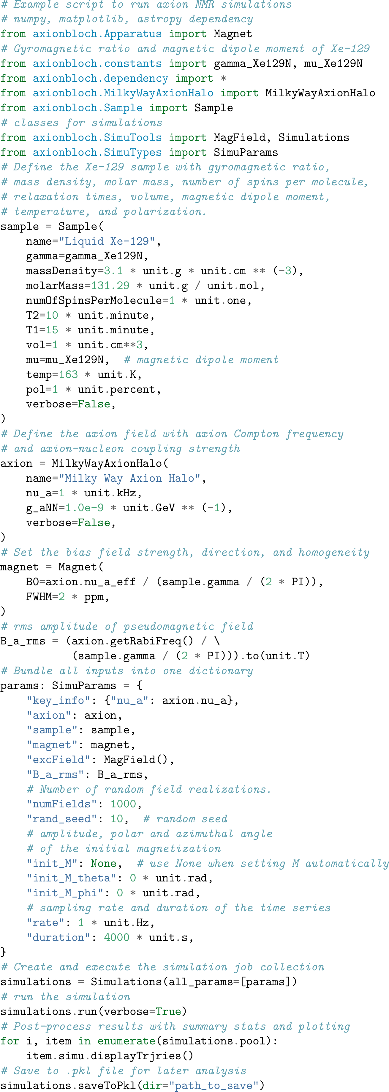
Figure 5: Example code of an axion simulation..
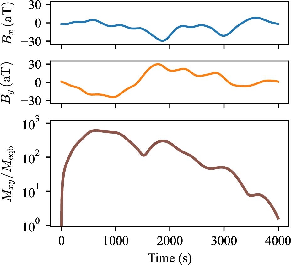
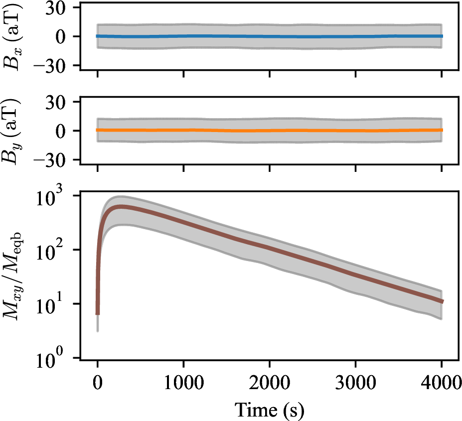
Figure 6: Simulations of local virialized axion dark matter halo. From top to bottom: pseudomagnetic fields in the transverse plane (\(B_x\) and \(B_y\)) and the transverse magnetization normalized by the equilibrium magnetization (\(M_{xy}/M_\mathrm{eqb}\)). Left: one single simulation. Right: 1000 simulations to account for the stochasticity. The solid lines indicate the value (left column) or mean value (right column) of \(B_x\), \(B_y\), and \(M_{xy}\), while the gray shadows indicate the \(\pm \sigma\) (standard deviation) range. The sample for the simulations is assumed to be polarized to \(\SI{50}{\%}\) initially..
3 Development↩︎
Development of is managed using git,4 with the code hosted on a public GitHub repository.5 Changes to the main codebase follow a pull request workflow, allowing contributions to be reviewed before being merged. Users can participate by forking the repository, making modifications in their fork, and
submitting pull requests for review by the developers. As is intended as a collaborative resource, user contributions and suggestions are encouraged and appreciated.
includes a suite of automated tests to ensure correctness and reliability. The tests are implemented using the pytest framework,6 which allows for calibration
of physical processes and testing of functions, classes, and modules. The test suite covers core functionalities such as:
initialization and manipulation of classes;
numerical integration of the Bloch equations;
magnetic fields and relaxations;
handling of each axion field configuration.
Tests can be executed locally. In the future, tools may be added for online testing considering the demand of testing.
Documentation for is available on Read the Docs.7 It is built using Sphinx8
and provides detailed explanations of the API, along with instructions for installation, configuration, and usage.
As numerous new axion models and experiments are emerging, the functionality of may extend so that it can be a tool for updating our knowledge of the induced spin dynamics. Furthermore, capabilities for simulating zero-to-ultra-low-field (ZULF) NMR will be implemented in future versions.
4 Conclusions↩︎
has been presented as a framework for simulating spin dynamics induced by magnetic fields or axion fields under a variety of physical scenarios. The package adopts SI units so that the inputs and outputs are directly comparable to experimental parameters and observables. Numerical integration of the Bloch equations is performed using a fourth-order Runge–Kutta method in the rotating coordinate frame, enabling stable and efficient simulation. Comprehensive calibrations have been performed to ensure the accuracy of the simulations. An example simulation of axion-induced signals from a local virialized axion dark matter halo is presented to demonstrate the package’s capabilities.
By providing an open-source, well-documented, and tested tool, aims to facilitate the study of axion-induced spin dynamics in precision measurement experiments and to serve as a platform for further method development and incorporation of new axion models.
Note that this package can be of interest to the NMR community for its applications in, for example, educational purposes. For example, students can specify pulse sequences for the simulation and see the visualized simulation results.
Data Availability↩︎
The data and code that generate this manuscript are available at https://github.com/Yuzhe98/AxionBloch-paper.
The author acknowledges helpful discussions with Hendrik Bekker, Dmitry Budker, and Alexander Sushkov, and thanks the CASPEr Collaboration for its support. The author is grateful to the communities supporting the open-source software and tools:
git, NumPy, SciPy9 [51], matplotlib10, astropy, pybind11, IPython11 [52], Jupyter12 [53], pytest, Sphinx, GitHub13 and Read the Docs14. This work has been supported by the Cluster of Excellence “Precision Physics, Fundamental
Interactions, and Structure of Matter” (PRISMA++ EXC 2118/2) funded by the German Research Foundation (DFG) within the German Excellence Strategy (Project ID 390831469).