Supplemental Material for “Dissipative preparation of Laughlin-like states”
June 22, 2026
1 Total correlation function↩︎
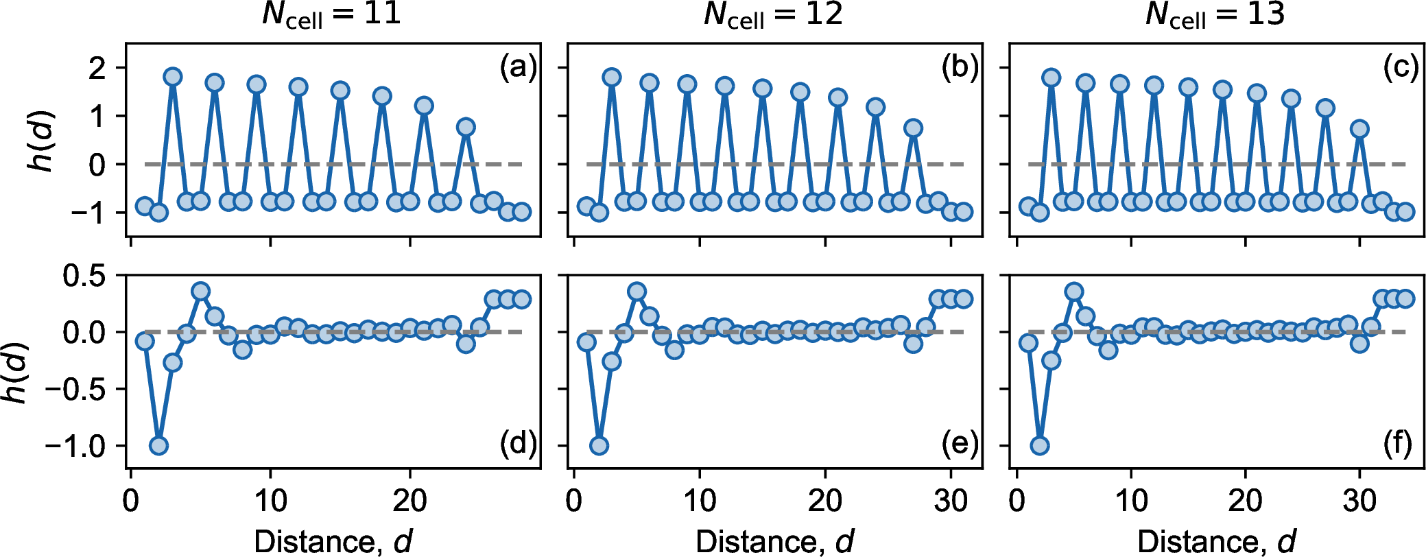
Figure 1 shows the total correlation function \(h(d) = g(d) - 1\) as a function of the separation distance \(d\) in the \(\nu=1/3\) Laughlin-like state. Results for \(\alpha=0.2\) and \(\alpha=1\) are shown in the first and the second rows, respectively. We define the radial distribution function \(g(d)\) as \[g(d) = \frac{1}{N_d}\frac{\sum_j^{N_d} \langle n_j n_{j+d}\rangle}{\bar n^2},\quad \bar n = \frac{1}{N}\sum_j \langle n_j\rangle,\] where \(N_d\) is the number of orbital pairs separated by \(d\). To mitigate boundary effects, the first and last orbitals are excluded from the evaluation of both \(g(d)\) and \(\bar n\).
For \(\alpha=0.2\), \(h(d)\) displays pronounced oscillations with period three, indicating a strong crystalline order. In contrast, for \(\alpha=1\), \(h(d)\) rapidly decays to zero in the bulk, consistent with liquid-like correlations. The weak upturn at large \(d\) originates from residual boundary effects when the separation becomes comparable to the total length.
2 Overlap between the Laughlin-like states and Laughlin states↩︎
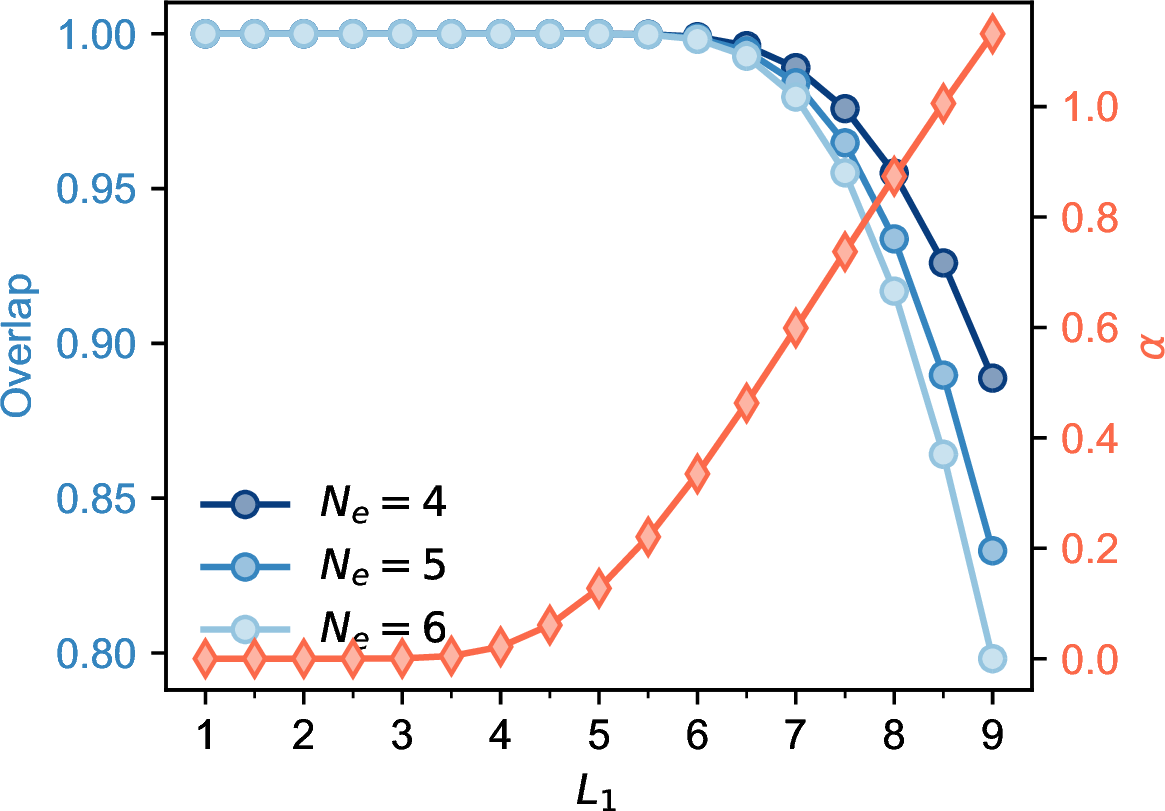
Figure 2 shows the overlap \(|\langle\psi_L|\psi_\mathrm{ss}\rangle|^2\) between the \(\nu=1/3\) Laughlin-like state \(|\psi_\mathrm{ss}\rangle\) in Eq. (5) of the main text and the exact Laughlin state \(|\psi_L\rangle\) on the cylinder with \(N_e=4\), 5, and 6. Using \(\alpha\) as a variational parameter, we find the maximum overlap at \(\alpha=3e^{-2\kappa^2}\) with \(\kappa=2\pi/L_1\). The overlap remains close to unity up to \(L_1\simeq 6\). Moreover, throughout \(0\le\alpha\le 1\), the Laughlin-like state maintains a high overlap with the exact Laughlin state.
3 Lindbladian gap↩︎
As in the main text, we focus on the Lindbladian gap with \(M=3\) in the parameter regime \(0\le \alpha \le 1\) and \(0 < \gamma \le 1\).
3.1 Tao-Thouless limit: \(\alpha = 0\)↩︎
In the Tao-Thouless (TT) limit, each jump operator \(V_j^m\) or \(W_j^m\) only involves a two-particle loss operator \(c_i c_j\). Along with the pump operator, for any Fock state \(|s\rangle\), each jump operator \(L_k\) sends it to another Fock state \(|t_k(s)\rangle\), i.e., \(L_k|s\rangle = \phi_k(s)|t_k(s)\rangle\) if \(\langle s|L_k^\dagger L_k|\rangle s\rangle = 1\) and \(L_k|s\rangle = 0\) otherwise, where \(\phi_k(s) = \pm 1\). Note that the recycling terms always change the particle number in double space by the same amount of particle \(|s\rangle\langle s'| \rightarrow |s-2\rangle\langle s'-2|\) or \(|s\rangle\langle s'| \rightarrow |s + 1\rangle\langle s'+1 |\) and the anti-commutator part preserves the particle number. The entire doubled Hilbert space can be split into two diagonal and off-diagonal subspaces. The eigenvalues of \(\mathcal{L}\) is thus the union of the eigenvalues of two blocks.
In the diagonal subspace \(\mathcal{X}\) with \(s = s'\), the Lindbladian acts as a classical Markov process generator. Let \(\mathcal{G}\) be the directional jump graph on Fock states with an edge between \((s, t_k(s))\) for every \((k, s)\) with \(\langle s|L_k^\dagger L_k|s\rangle = 1\). Then \(\mathcal{G}\) is acyclic and has no self-loops since pump operators can only replenish particles separated by \((M-1)\) orbitals while the loss operators deplete particles occupying at nearest-neighboring (NN) or next-nearest-neighboring (NNN) orbitals. By applying Kahn’s algorithm for a directional acyclic graph, the Fock states \(\{s\}\) can be relabeled as \(s_1, s_2, \dots, s_{2^{N_\phi}}\) such that every transition \(s_i \rightarrow s_j\) driven by a jump operator satisfies \(i < j\). Therefore, \({\mathcal{L}}\big\vert_\mathcal{X}\) can be rewritten as a lower-triangle matrix in this ordering. The eigenvalues are given by the diagonal elements which are contributed by the anti-commutator part \(-\frac{1}{2}\left\{H_\mathrm{eff}, \cdot\right\}\) of the Lindbladian with \[H_\mathrm{eff} = \sum_{j=0}^{N_\phi-2} n_j n_{j+1} + \sum_{j=0}^{N_\phi-3}n_j n_{j+2} + \gamma\sum_{j=1}^{N_\mathrm{cell}}n^h_j,\label{eq:diag95ham}\tag{1}\] where \(n^h_j\) denotes the local hole number (0 or 1) at the cell \(j\). \(H_\mathrm{eff} \ge 0\) as each term in Eq. (1 ) is a projector. The null space of \(H_\mathrm{eff}\) is one-dimensional and spanned by the TT state. When \(\gamma < 1\), the smallest non-zero eigenvalue of \(H_\mathrm{eff}\) is \(\gamma\), corresponding to one local hole in the TT state. Taking \(N_\mathrm{cell}=3\) as an example, the null space only contains the TT state \(|0, 3, 6\rangle\) but the one-local-hole subspace is ten-fold degenerate, spanned by the states \(|0, 3\rangle\), \(|1, 4\rangle\), \(|2, 5\rangle\), \(|2, 6\rangle\), \(|3,6\rangle\), \(|0, 4\rangle\), \(|0, 5\rangle\), \(|0, 6\rangle\), \(|1,6\rangle\) and \(|1, 5\rangle\). The largest non-zero eigenvalue of \({\mathcal{L}}\big\vert_\mathcal{X}\) is thus \(-\gamma\).
In the off-diagonal subspace \(\mathcal{Y}\), the Lindlbian acts on \(|s\rangle\langle s'|\) \((s\ne s')\) as \[\mathcal{L}(|s\rangle\langle s'|) = -\frac{1}{2}\left(E(s) + E(s')\right)|s\rangle\langle s'| + \sum_k \phi_k(s)\phi_k(s')c_k(s)c_k(s')|t_k(s)\rangle\langle t_k(s')|, \label{eq:lin95off95diag}\tag{2}\] where \(E(s) = \langle s|H_\mathrm{eff}|s\rangle\) and \(c_k(s) = \langle s| L_k^\dagger L_k|s\rangle\). Define the doubled jump graph \(\mathcal{G}^{(2)}\) on pairs \((s, s')\) with an edge \((s, s') \rightarrow (t_k(s), t_k(s'))\) for every \(k\) with \(c_k(s) c_k(s') = 1\) and \(s \ne s'\). Similarly, the graph \(\mathcal{G}^{(2)}\) is also acyclic because a cycle in \(\mathcal{G}^{(2)}\) projects to a closed walk on the first coordinate in \(\mathcal{G}\) which contradicts the acyclicity of \(\mathcal{G}\). Therefore, the second term in Eq. (2 ) is strictly lower-triangle after employing Kahn’s algorithm to relabel the pairs \((s, s')\). The eigenvalues of \({\mathcal{L}}\big\vert_\mathcal{Y}\) is read off the diagonal: \[-\frac{1}{2} \left(E(s) + E(s')\right),\quad s\ne s'.\] The largest non-zero eigenvalue is \(-\gamma/2\) obtained when \(\{E(s), E(s')\} = \{0, 1\}\).
Combining the results of two subspaces, the gap \(\Delta\) of Lindbladian is thus \(\gamma/2\).
3.2 Beyond the Tao-Thouless limit: \(0 < \alpha \le 1\)↩︎
Inspired by the former case, we examine the excitation gap \(\Delta^\mathrm{exc}\) of the effective Hamiltonian \(H_\mathrm{eff} = \sum_k L_k^\dagger L_k\) \[\begin{align} H_\mathrm{eff} &= H_\mathrm{loss} + H^h, \notag \\ H_\mathrm{loss} &= \sum_{j=0}^{N_\phi- 2}n_j n_{j+1} + \sum_{j=0}^{N_\phi - 3}n_j n_{j+2} + \alpha^2\sum_{j=0}^{N_\phi - 4}n_j n_{j+3} + \alpha\sum_{j=0}^{N_\phi-4} \left( c_{j+3}^\dagger c_j^\dagger c_{j+1} c_{j+2} + \mathrm{h.c.}\right),\notag \\ H^h &= \gamma\sum_{j=1}^{N_\mathrm{cell}} n_j^h . \end{align}\] The steady state \(|\psi_\mathrm{ss}\rangle\) of \(H_\mathrm{eff}\) is given by Eq. (5) in the main text. By denoting the first excited state of \(H_\mathrm{eff}\) as \(|\psi_\mathrm{ss}^{\mathrm{exc},(1)}\rangle\), \(|\psi_\mathrm{ss}\rangle\langle\psi_\mathrm{ss}^{\mathrm{exc,(1)}}|\) is the eigenoperator of \(\mathcal{L}\) since \[\begin{align} \mathcal{L}(|\psi_\mathrm{ss}\rangle\langle\psi_\mathrm{ss}^{\mathrm{exc}, (1)}|) ={}& \sum_{k} L_k |\psi_\mathrm{ss}\rangle\langle\psi_\mathrm{ss}^{\mathrm{exc}, (1)}|L_k^\dagger - \frac{1}{2}H_\mathrm{eff}|\psi_\mathrm{ss}\rangle\langle\psi_\mathrm{ss}^{\mathrm{exc}, (1)}| - \frac{1}{2}|\psi_\mathrm{ss}\rangle\langle\psi_\mathrm{ss}^{\mathrm{exc}, (1)}|H_\mathrm{eff} \notag \\ ={}&-\frac{\Delta^\mathrm{exc}}{2}|\psi_\mathrm{ss}\rangle\langle\psi_\mathrm{ss}^{\mathrm{exc}, (1)}|. \end{align}\] The cycling terms vanish because \(L_k|\psi_\mathrm{ss}\rangle = 0\). Similarly, \(|\psi_\mathrm{ss}^{\mathrm{exc},(1)}\rangle\langle\psi_\mathrm{ss}|\) is another eigenoperator of \(\mathcal{L}\) with the same eigenvalue \(-\Delta^{\mathrm{exc}} / 2\). As \(\Delta^\mathrm{exc}\) controls the Lindbladian gap, we first examine the gap of the effective Hamiltonian.
3.3 The gap of the effective Hamiltonian↩︎
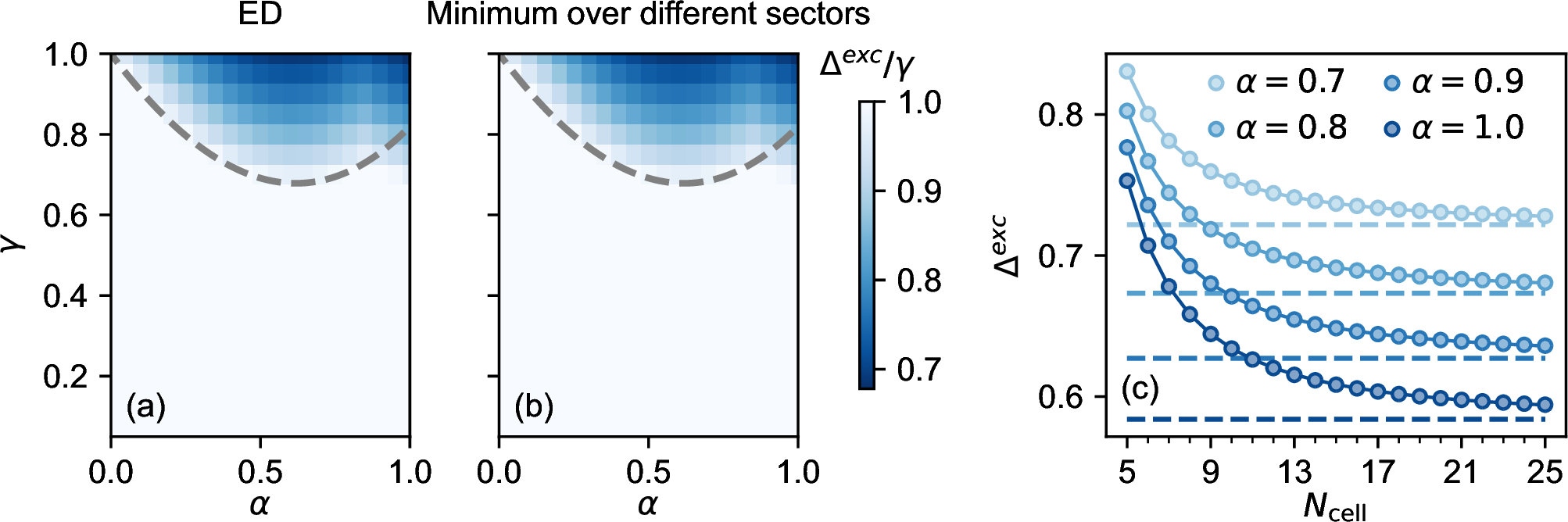
As shown in the Fig. 3(a) of the main text, the Lindbladian gap \(\Delta\) is set by the lowest of three branches. We first consider the one-local-hole sector, in which the steady state contains one local hole. Since the local-hole states are also annihilated by the two-particle loss operators, only \(H^h\) contributes to the excitation energy. Accordingly, the one-local-hole excitation energy is \(\gamma\) and the gap \(\Delta\) is given by \(\gamma/2\).
Since the effective Hamiltonian converses the total momentum, we consider the sector with the momentum change \(\Delta K = 1\) with respect to the TT state. Starting from the root state \(|0, 3, 5, \dots \rangle\), the minimal realization appears in the three-dimensional subspace spanned by the states \(|0, 3, 5,\dots\rangle\), \(|1, 2, 5,\dots\rangle\), \(|1, 3, 4,\dots\rangle\), and is described by the Hamiltonian \(H^\mathrm{defect}\) \[\begin{pmatrix} 1 + \alpha^2 & \alpha & 0 \\ \alpha & 1 + \alpha^2 & \alpha \\ 0 & \alpha & 2 + \alpha^2 + \gamma \end{pmatrix}.\] Requiring the smallest eigenvalue \(\lambda_1\) to satisfy \(\lambda_1 > \gamma\), we obtain \[\gamma < \frac{2\alpha^4 +5\alpha^2 + 4 - \alpha\sqrt{4\alpha^4 + 17\alpha^2 + 16}}{2(\alpha^2 + 2)}.\label{eq:boundary}\tag{3}\] The local defect block is decoupled from the remaining part with two permanently empty buffer orbitals \(7\) and \(8\). No allowed four-site pattern \(1001\) or \(0110\) can cross this buffer. The full Hilbert space thus factorizes as \(\mathcal{H}^\mathrm{defect}\otimes \mathcal{H}^\mathrm{tail}\), and the effective Hamiltonian decouples into \(H^\mathrm{defect} + H_\mathrm{eff}^\mathrm{tail}\). Since \(H_\mathrm{eff}^\mathrm{tail}\) is positive, the smallest eigenvalue of \(H_\mathrm{eff}\) coincides with the smallest eigenvalue \(\lambda_1\) of \(H^\mathrm{defect}\).
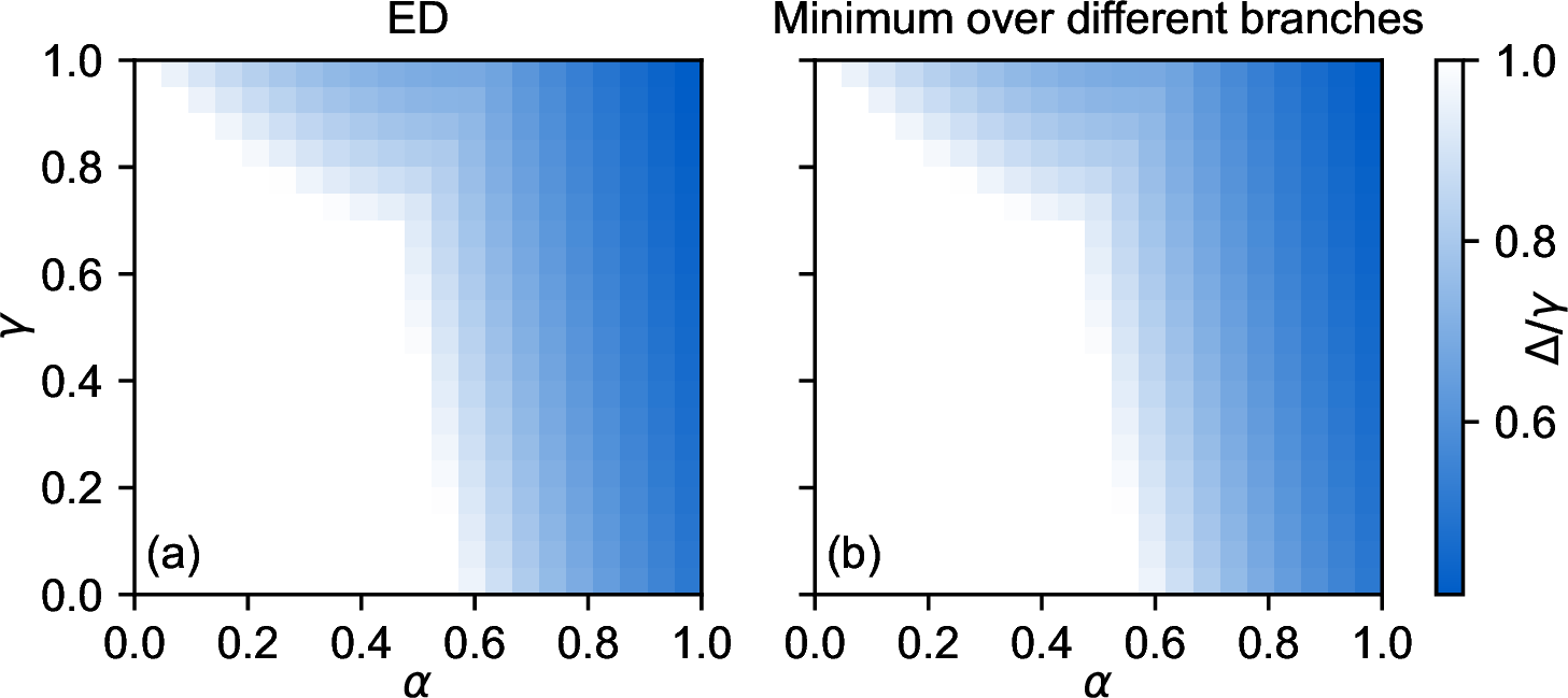
Figure 3 (a) shows the gap as a function of \(\alpha\) and \(\gamma\), obtained by exact diagonalization for \(N_\mathrm{cell}=7\) and \(N_s=19\). Dividing the gap by \(\gamma\) makes the crossover between the \(\gamma-\)dominated and \(\lambda_1\)-dominated regions clearly visible. The boundary is given by Eq. (3 ).
3.4 The gap in the sector \(\Delta K = 0\)↩︎
The upper-right corner of Fig. 3 (a), however, deviates from \(\lambda_1\), indicating the presence of another type of excitation in the sector \(\Delta K = 0\). In this sector, there are neither holes nor particle pairs separated by a distance of 2, so the gap is fully determined by \[\sum_j n_j n_{j+1} + \alpha^2\sum_j n_jn_{j+3} + \alpha\sum_j\left(c_{j+3}^\dagger c_j^\dagger c_{j+1} c_{j+2} + \mathrm{h.c.}\right)\label{eq:eff95ham95k0} .\tag{4}\] Figure 3 (c) shows the gap in the sector \(\Delta K=0\) as a function of \(N_\mathrm{cell}\) for several values of \(\alpha\). Each curve is well fitted by the function \(\Delta^\mathrm{exc} = \Delta_\infty^\mathrm{exc} + a / N_\mathrm{cell}^b\) with fitting variables \((\Delta_\infty^\mathrm{exc}, a, b)\).
The gap can be explained by the equivalent Glauber dynamics. We define an effective variable \(x_k \in \{0, 1\}\), \(k = 1, \dots, N_\mathrm{cell}-1\), where \(x_k = 1\) means the \(k\)-th local pattern has jumped: \(1001\rightarrow 0110\). Two neighboring jumps cannot both occur, so \(x_k x_{k+1}=0\). Thus the effective configurations are exactly \[\Omega = \{x\in \{0, 1\}^{N_\mathrm{cell}-1}: x_k x_{k+1} = 0\}.\] These are the independent sets of the path graph \(\mathcal{G}\). The condition \(x_k x_{k+1} = 0\) is the hard-core constraint. We define \(|x| = \sum_k x_k\) which counts the number of effective jumps performed. Let \(A\) be the adjacency matrix of the one-jump between configurations in the graph. \(A(x,y) = 1\) if and only if \(x\) and \(y\) differ by flipping one \(x_k\), and \(x\) and \(y\) are allowed. Otherwise \(A(x, y) = 0\). For any \(x \in \Omega\), define \[C_1(x) = \#\{k: x_k=1\}, \quad C_0(x) = \#\{k: x_k = 0, \;x_{k-1} = 0, \;x_{k+1} = 0\}.\] Here \(C_1(x)\) counts allowed annihilation moves \(1\to 0\), and \(C_0(x)\) counts allowed creation moves \(0 \to 1\). Then the Hamiltonian in Eq. (4 ) can be expressed as \[H_\alpha(x,y)= \begin{cases} W_\alpha(x) = C_1(x) + \alpha^2 C_0(x),&x=y,\\ \alpha, &x \sim y,\\ 0,&\text{otherwise}, \end{cases}\] since a local \(0110\) pattern contributes \(1\), while a local \(1001\) pattern contributes \(\alpha^2\). \(x\sim y\) means that \(x\) and \(y\) are connected by one allowed effective flip. For simplicity, we define the sign-transformed matrix \[M_\alpha = U H_\alpha U^{-1} = W_\alpha - \alpha A,\] where \(U|x\rangle = (-1)^{|x|}|x\rangle\). By defining the projector \(P_k\) at the site \(k\) \(P_k = |0_k\rangle\langle 0_k|\), \(M_\alpha\) can be rewritten as \[M_\alpha = \sum_k P_{k-1} \begin{pmatrix} \alpha^2 & -\alpha \\ -\alpha & 1 \\ \end{pmatrix} P_{k+1}.\] The \(2\times 2\) matrix is positive semidefinite as \[\begin{pmatrix} \alpha^2 & -\alpha \\ -\alpha & 1 \\ \end{pmatrix} = \begin{pmatrix} \alpha \\ -1 \end{pmatrix} \begin{pmatrix} \alpha & -1 \end{pmatrix}.\] The zero-energy ground state is \[|\Psi_\alpha\rangle = \sum_{x\in \Omega} \alpha^{|x|}|x\rangle.\]
The hard-core Gibbs measure with fugacity \(\lambda > 0\) on the path \(\mathcal{G}\) is the probability measure on independent sets \[\mu_\lambda(x) = \frac{\lambda^{|x|}}{Z(\lambda)},\quad Z(\lambda) = \sum_{x\in \Omega}\lambda^{|x|}.\] In our case we set \(\lambda = \alpha^2\). The ground-state amplitudes are proportional to \(\sqrt{\mu_{\alpha^2}(x)}\). We can show that the measure \(\mu_{\alpha^2}\) can be generated by a heat-bath Glauber generator. If one of the neighbors of \(k\) is occupied, then \(x_k = 0\) forced by the hard-core constraint. If both neighbors are empty, then set \(x_k = 1\) with probability \(\alpha^2/(1 + \alpha^2)\) and set \(x_k = 0\) with probability \(1/(1+\alpha^2)\). The continuous-time generator \(Q\) is \[Q(x, y) = \begin{cases} \dfrac{\alpha^2}{1 + \alpha^2}, & y = x^k, \;x_k = 0, \;x_{k-1} = x_{k+1} = 0, \\[1.2em] \dfrac{1}{1 + \alpha^2}, & y = x^k, \;x_k = 1, \\[1.2em] -\displaystyle\sum_{z\ne x} Q(x, z), & y = x, \\ 0, & \text{otherwise.} \end{cases}\] Here again \(x_0 = x_{N_\mathrm{Ncell}} = 0\) at the boundaries. Thus \(Q\) is exactly the heat-bath Glauber generator for the hard-core Gibbs measure \(\mu_{\alpha^2}\). It satisfies detailed balance: \[\mu_{\alpha^2}(x)Q(x, y) = \mu_{\alpha^2}(y)Q(y, x).\] For example, if \(y = x^k\) is obtained from \(x\) by a \(0\to 1\) flip, then \(\mu_{\alpha^2}(y)/\mu_{\alpha^2}(x) = \alpha^2\), while \[\frac{Q(x, y)}{Q(y, x)} = \frac{\alpha^2/(1+\alpha^2)}{1/(1 + \alpha^2)} = \alpha^2.\] Therefore, the detailed balance condition holds.
To connect the generator \(Q\) with the matrix \(M_\alpha\), we show that \[Q = -\frac{1}{1 + \alpha^2} D_\mu^{-1/2}M_\alpha D_\mu^{1/2},\quad D_u(x, x) = \mu_{\alpha^2}(x).\label{eq:sym95Q}\tag{5}\] \(Q(x,y)\) and \(M_\alpha(x,y)\) are both nonzero only when \(x\sim y\). Suppose \(y = x^k\) with \(x_k = 0\) and \(y_k=1\). Substituting \(M_\alpha(x, y) = -\alpha\) and \(\sqrt{\mu_{\alpha^2}(y)/\mu_{\alpha^2}(x)} = \alpha\) into Eq. (5 ) yields \[Q(x, y) = \frac{\alpha^2}{ 1 + \alpha^2},\] which coincides with the definition of \(Q\). Similarly, we can also verify that Eq. (5 ) holds for \(x_k=1\) and \(y_k=0\). For \(y=x\), we have \[Q(x,x) = -\frac{C_1(x) + \alpha^2 C_0(x)}{1+\alpha^2}.\] which is exactly the sum of all outgoing rates from \(x\), \(\sum_{y\ne x} Q(x, y)\). We now consider the spectrum of the generator \(Q\) since \(Q\) and \(M_\alpha\) share the same spectrum according to Eq. (5 ).
Let \(K_k\) be the local update kernel at site \(k\). A discrete-time random-scan Glauber transition matrix is given by \[P_\mathrm{disc} = \frac{1}{N_\mathrm{cell} - 1}\sum_k K_k.\] It means that one site is uniformly picked at random, and is updated by the local kernel \(K_k\). The continuous-time generator \(Q\) is defined as \[Q = \lim_{dt\rightarrow 0}\frac{P_{dt} - 1}{dt},\quad P_t(x,y) = \mathrm{Pr}(X_t=y|X_0=x).\] Because the local sites are independent, the transition probability during a short duration \(dt\) is \[P_{dt} = (1 - (N_\mathrm{cell}-1)dt)I + \sum_k K_k dt + O(dt^2) = I + \sum_{k}(K_k - I)dt + O(dt^2).\] Therefore \[Q = \sum_{k=1}^{N_\mathrm{cell}-1}(K_k - I) = (N_\mathrm{cell}-1)(P_\mathrm{disc} - I).\] The continuous-time spectral gap is \((N_\mathrm{cell}-1)\) times the discrete-time spectral gap.
The recent result of Glauber dynamics states that [1], for antiferromagnetic two-spin systems in the tree-uniqueness regime, the discrete-time Glauber dynamics has an optimal \(\Omega(n^{-1})\) lower bound on the spectral gap; for the hard-core model with fugacity \(\lambda\) and maximum degree \(D\), one sufficient condition is \[\lambda\le(1-\delta)\lambda_c(D), \qquad \lambda_c(D)=\frac{(D-1)^{D-1}}{(D-2)^D}, \label{eq:uniqueness-condition}\tag{6}\] for some fixed \(\delta\in(0,1)\).
Our effective graph is a path, so it has maximum degree \(2\). To use the standard theorem stated for maximum degree at most \(D\ge3\), we may embed the path class into the class of graphs with maximum degree at most \(3\). Then the sufficient condition becomes \(\lambda < 4\), which is equivalent to \(\alpha < 2\). For such fixed \(\alpha\), choose \(\delta=1-\frac{\alpha^2}{4}>0\). The theorem gives a constant \(c(\alpha)>0\), independent of the system size, such that \[\mathrm{gap}_{\mathrm{disc}}\ge \frac{c(\alpha)}{N_\mathrm{cell}-1}\] We thus prove that the gap of the generator \(Q\) is greater than \(c(\alpha)\) for every fixed \(0<\alpha<2\).
From another perspective, the Hamiltonian in Eq. (4 ) is the parent Hamiltonian of an injective matrix product state (MPS). The MPS for the ground state has bond dimension 2, \[M^{(r)} = \begin{pmatrix} 1 & 0 \\ 1 & 0 \end{pmatrix},\quad M^{(d)} = \begin{pmatrix} 0 & -\alpha \\ 0 & 0 \end{pmatrix},\] where each bond is either a rod state \(|r\rangle = |1001\rangle\) or a dimer state \(|d\rangle = |0110\rangle\). Since the products of these matrices span all \(2\times 2\) matrices, the MPS is injective. A frustration-free parent Hamiltonian of an inject MPS has a unique ground state and a spectral gap bounded below by a positive constant independent of system size [2]. Hence \(H\) is gapped in the sector \(\Delta K = 0\).
Figure 3 (b) shows the minimum of the three gaps in the sectosr \(\Delta K = 0\) and \(\Delta K = 1\), together with \(\gamma\), which agrees with the ED result, confirming that these three gaps entirely capture the spectral gap throughout the parameter range \(0 \le \alpha \le 1\) and \(0<\gamma\le 1\).
3.5 The gap of \(\mathcal{L}\) in the invariant subspace↩︎
| \(\alpha=0.65\) | \(\alpha=0.85\) | \(\alpha=1\) | |
|---|---|---|---|
| \(\gamma=0.05\) | (0.0186, 0.0294, 1.528) | (0.0118, 0.0305, 1.393) | (0.00798 , 0.0299, 1.295) |
| \(\gamma=0.5\) | (0.161, 0.290, 1.562) | (0.103, 0.295, 1.449) | (0.0723, 0.289, 1.368) |
| \(\gamma=1.0\) | (0.275, 0.540, 1.577) | (0.181, 0.548, 1.474) | (0.129, 0.546, 1.411) |
Starting from the vacuum state \(|0\dots0\rangle\langle 0\dots 0|\), the system traverses a subspace through a sequence of jumps induced by \(\mathcal{L}\). During this process, no two particles ever occupy orbitals separated by a distance of two since particles are only replenished in the orbitals \(3j\) with \(j = 0, 1, 2, \dots, N_\mathrm{cell}-1\). Therefore, the gap within this subspace is independent of the jump operators \(c_j c_{j+2}\), which can be removed from the Lindbladian. We generate all such states by repeatedly applying the Lindbladian and then diagonalize it in the basis of doubled Fock states spanning these states.
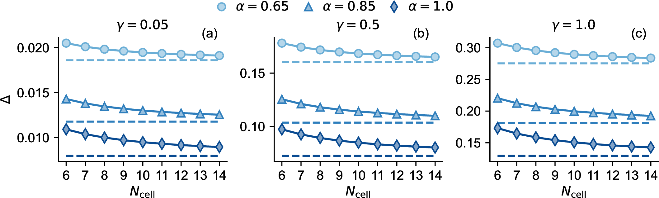
Figure 4 shows the Lindbladian gap in the invariant subspace as a function of \(N_\mathrm{cell}\) for several values of \((\alpha, \gamma)\). Each data series is also well fitted by \(\Delta_\infty + a / N_\mathrm{Ncell}^b\) with the fitting coefficients \((\Delta_\infty, a, b)\) reported in Table 1. As shown in each row of Table 1, the coefficient \(a\) strongly depends on \(\gamma\) and is essentially independent of \(\alpha\), while the exponent \(b\) lies in the range \([1, 2]\). Taking the mininum of the Lindbladian gap in the invariant subspace and \(\Delta^\mathrm{exc}/2\) yields Fig. (3)a in the main text. Figure 5 compares the gap obtained by exact diagonalization with the minimum over all branches. The two results agree to within numerical precision in the regions \(0\le \alpha \le 1\) and \(0 < \gamma \le 1\). We note that \(\Delta^\mathrm{exc}\) in the sector \(\Delta K = 0\) exceeds twice the Lindbladian gap in the restricted subspace in the right upper corner of the diagram (\(0.6 < \alpha \le 1\) and \(0.5 \le \gamma \le 1\)). The Lindbladian gap is thus governed by the effective Hamiltonian gap \(\Delta^\mathrm{exc}\) only in regions \(A\) and \(B\), as shown in Fig. 3(a) of the main text.
4 Adiabatic pump↩︎
The Lindbladian gap \(\Delta(t)\) over one period is shown as a function of \(t/T\) in Fig. 6. It reaches the minimum \(\Delta/\gamma\approx 0.22\) at \(t/T=0.5\), coinciding with the minimum point of the scale factor \((1-t/T)^2 + (t/T)^2\).
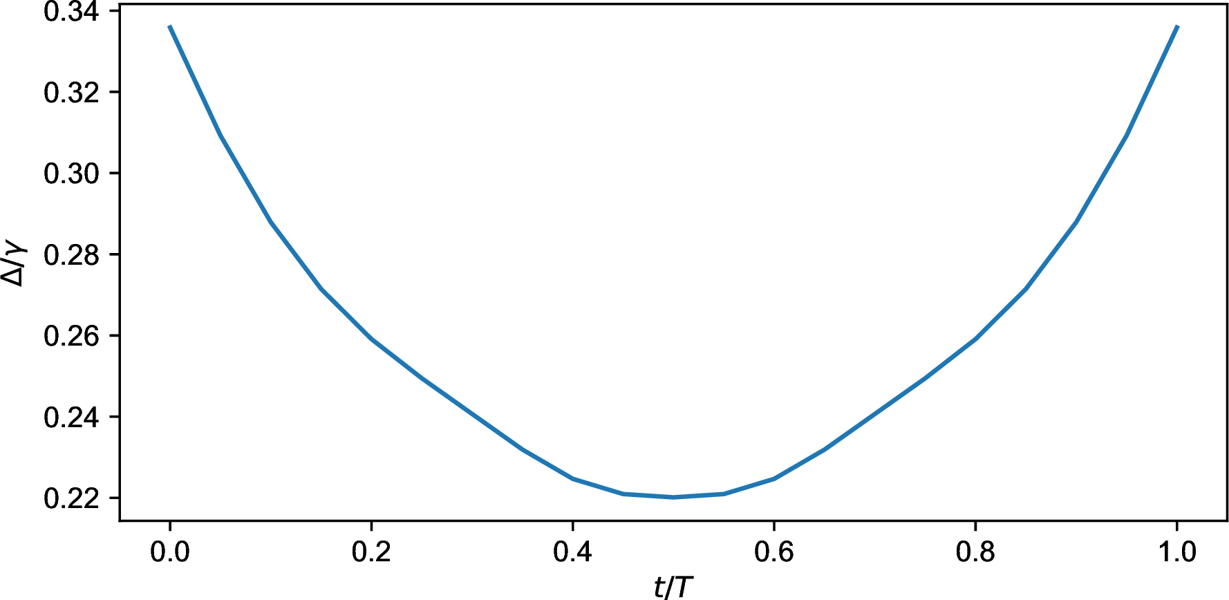
For the maximal pump strength \(\gamma=1\), we choose \(T = 40\) to ensure \(T \gg 1/\Delta\).
The boundary contribution to the adiabatic error can be estimated from the rate of change of \(\mathcal{L}_i(t)\) at the endpoint \(t=T\) in the \(i\)-th period, \[c_m = \mathrm{Tr}\left[\sigma_m^\dagger \partial_t \mathcal{L}_i(t)(\rho_\mathrm{ss})\right]\big\vert_{t=T}\] where \(\rho_\mathrm{ss}\) is the steady state of \(\mathcal{L}_i(t)\) at \(t=T\) and \(\sigma_m\) is the \(m\)-th left eigenoperator. For the quadratic path, the derivative is given by \[\partial_t \mathcal{L}_i(t)\vert_{t=T} = \mathcal{\mathcal{\mathcal{Q}}}_{i+1},\] where \(\mathcal{Q}_{i+1}\) is the pump dissipator at \(t=T\) of the \(i\)-th period. Since \(Q_{i+1}\) annihilates \(\rho_\mathrm{ss}\), we obtain \(c_m = 0\).
5 Preparation of \(\nu=1/2\) Laughlin-like states↩︎
The target \(\nu=1/2\) Laughlin-like states with \(N_\phi = 2N_e - 1\) is expressed as \[|\psi\rangle = \prod_j \left(1 - \frac{\alpha}{2}a_{j-1}a_{j+1}{a_j^{\dagger}}^2\right)|\psi_\mathrm{TT}\rangle,\label{eq:bosonic95FQH}\tag{7}\] where \(a_j\) (\(a_j^\dagger\)) is the bosonic annihilation (creation) operator at the orbital \(j\), and the corresponding TT state is \(|1010\cdots 101\rangle\). The inward squeezing operator moves two adjacent bosons toward the central orbital, creating a doublon.
For fermionic states, the two-particle loss operators \(V_j^m\) start from \(\zeta_j^1 c_{j-1}c_{j+1}\), whereas for bosonic states they start from \(\zeta_j^0 a_j^2\), since two bosons can occupy the same orbital. Moreover, in the bosonic case, squeezing occurs only between orbitals separated by an even number of orbitals. The squeezed states are thus induced by the associated loss operators \(V_j^m = \zeta_j^0 a_j^2 + \alpha \zeta_j^1 a_{j-1}a_{j+1}\) rather than by \(W_j^m\) as in the fermionic case.
The pump operators take the same form as in the fermionic case, but overlap between neighboring operators. Taking \(N_e=3\) and \(N_\phi=5\) as an example, the pump operators include \(a_0^\dagger P_1\), \(P_1a_2^\dagger P_3\), \(P_3 a_4^\dagger\) where \(P_i\) is the projector onto the Fock state \(|0_i\rangle\).
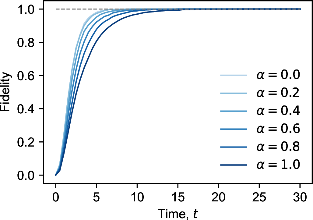
Figure 7 shows the fidelity between the target state Eq. (7 ) and the evolved state as a function of time, starting from the vacuum state. States with larger \(\alpha\) take longer to reach unit fidelity, similar to the fermionic case.
6 Experimental realization↩︎
6.1 Physical setting and notation↩︎
We consider a one-dimensional array of frozen target tweezers with lattice spacing \(s\) and spin-polarized fermions. We denote by \(c_j^\dagger\) the creation operator for a spin-polarized fermionic atom in the selected ground-state motional orbital of tweezer \(j\). The corresponding operators satisfy \(\{c_i,c_j^\dagger\}=\delta_{ij}\). The target tweezers are assumed sufficiently deep and well separated that coherent tunnelling between target sites is negligible during the dissipative evolution. The central auxiliary object is a Rydberg macrodimer mode. For a pair of sites \((j,k)\) separated by \[R_{jk}=|x_j-x_k| ,\] we denote by \(d_{jk,\alpha}^\dagger\) the creation operator of a macrodimer in vibrational/electronic branch \(\alpha\), with centre of mass near \((x_j+x_k)/2\) and relative coordinate localized near the molecular bond length. The operator \(d_{jk,\alpha}^\dagger\) does not create an ordinary atom on an auxiliary site. It creates a two-atom Rydberg molecular excitation associated with the pair \((j,k)\). Since it contains two fermions, it is bosonic to a good approximation in the low-excitation manifold.
The target dissipator we seek is \[\dot{\rho} = \sum_{j,r} \Gamma_r\,{\mathcal{D}}[c_jc_{j+r}](\rho) , \label{eq:target95dissipator}\tag{8}\] where \({\mathcal{D}}[L](\rho) = L\rho L^\dagger - \frac{1}{2}\left\{L^\dagger L,\rho\right\}\). For \(r=1\) this is nearest-neighbour pair loss, and for \(r=2\) it is next-nearest-neighbour pair loss. In one dimension, the fermionic signs associated with \(c_jc_{j+r}\) are fixed by the chosen site ordering. For a dissipator \({\mathcal{D}}[c_jc_{j+r}]\), an overall sign of the jump operator is immaterial.
6.2 Macrodimer association and distance selectivity↩︎
At the effective level, the association process is described by \[H_{\rm assoc}^{(\alpha)} = \hbar \sum_{j<k} \left[ g_\alpha(R_{jk}) d_{jk,\alpha}^\dagger c_j c_k + {\rm H.c.} \right] + \hbar \sum_{j<k} \delta_\alpha(R_{jk}) d_{jk,\alpha}^\dagger d_{jk,\alpha}. \label{eq:macrodimer95effective95association}\tag{9}\] Here \(g_\alpha(R_{jk})\) is the effective two-atom association matrix element, including the optical Rabi frequencies and the Franck–Condon overlap between the pinned atom-pair wavefunction and the selected macrodimer wavefunction. The detuning \[\delta_\alpha(R) = 2\varepsilon_\alpha + \frac{U_{u_\alpha}(R)}{\hbar} + \delta_{\rm AC}^{(\alpha)} \label{eq:macrodimer95distance95detuning}\tag{10}\] is the two-photon detuning from the molecular resonance. In this expression, \(\varepsilon_\alpha\) is the single-atom detuning of tone \(\alpha\) from the bare Rydberg transition, \(U_{u_\alpha}(R)\) is the Rydberg-pair molecular potential for the selected branch \(u_\alpha\), and \(\delta_{\rm AC}^{(\alpha)}\) denotes light shifts and other experimentally calibrated offsets. The sign convention in Eq. 10 is not essential; what matters is that the resonance condition is \[\delta_\alpha(R)=0 . \label{eq:macrodimer95resonance95condition}\tag{11}\]
Equation 11 is the origin of distance selectivity. Since \(U_{u_\alpha}(R)\) depends strongly on the interatomic separation, changing the tone frequency changes which separation is resonant. In a uniform one-dimensional array with neighbouring tweezer spacing \(s\), a tone satisfying \[2\varepsilon_1+\frac{U_{u_1}(s)}{\hbar}\simeq0 \label{eq:NN95macrodimer95resonance}\tag{12}\] addresses nearest-neighbour pairs \((j,j+1)\), whereas a second tone satisfying \[2\varepsilon_2+\frac{U_{u_2}(2s)}{\hbar}\simeq0 \label{eq:NNN95macrodimer95resonance}\tag{13}\] addresses next-nearest-neighbour pairs \((j,j+2)\). Thus the frequency of the association tone selects a class of pair separations rather than a unique bond. A global tone resonant at \(R=s\) couples to all illuminated nearest-neighbour bonds, while a global tone resonant at \(R=2s\) couples to all illuminated next-nearest-neighbour bonds.
The association strength is appreciable only when the pinned atom pair has non-negligible overlap with the selected macrodimer wavefunction. We may write schematically \[g_\alpha(R) \propto \Omega_\alpha^{\rm eff} \eta_{u_\alpha}(R), \label{eq:FC95pair95coupling}\tag{14}\] where \(\Omega_\alpha^{\rm eff}\) contains the relevant optical coupling strengths and \(\eta_{u_\alpha}(R)\) is a Franck–Condon factor. The sharp dependence of both \(\delta_\alpha(R)\) and \(\eta_{u_\alpha}(R)\) on \(R\) underlies the experimentally observed distance selectivity of macrodimer excitation and dressing [3], [4]. In practice, the usable selectivity is limited by the molecular linewidth, the association Rabi frequency, the motional width of the pinned atoms, and possible off-resonant coupling to nearby vibrational resonances.
For a spatially uniform drive, Eq. 9 should be understood as a sum over local macrodimer modes. A nearest-neighbour tone and a next-nearest-neighbour tone generate \[H_{\rm assoc}^{(1)} = \hbar \sum_j \left[ g_1 d_{j,j+1}^{(1)\dagger}c_jc_{j+1} + g_2 d_{j,j+2}^{(2)\dagger} c_j c_{j+2} + {\rm H.c.} \right] + \hbar \sum_j \delta_1 d_{j,j+1}^{(1)\dagger}d_{j,j+1}^{(1)} + \sum_j \delta_2 d_{j,j+2}^{(2)\dagger}d_{j,j+2}^{(2)} . \label{eq:NN95effective95macrodimer95association}\tag{15}\] The internal molecular resonance is the same on every bond, but \(d_{j,j+1}^{(1)}\) and \(d_{j+1,j+2}^{(1)}\) are distinct local modes with different centre-of-mass positions.
6.3 Converting the macrodimer into a lossy auxiliary mode↩︎
To realize irreversible two-body loss, the macrodimer mode must be made short-lived. We write the molecular decay as \(\kappa_\alpha {\mathcal{D}}[d_{jk,\alpha}](\rho)\). The linewidth \(\kappa_\alpha\) may contain intrinsic Rydberg decay, motional escape from the trap, photoionization, or an engineered dump channel. A useful controlled mechanism is to apply an additional dump tone coupling the macrodimer state \(|M\rangle\) to a rapidly decaying state \(|B\rangle\), \[|M_{jk}^{(u_\alpha)}\rangle \xrightarrow{\Omega_{D,\alpha}} |B_{jk}\rangle \xrightarrow{\gamma_B}{\mathrm {loss}}.\] The corresponding Hamiltonian is \[H_D/\hbar = \Delta_B |B\rangle\langle B| + \frac{\Omega_{D,\alpha}}{2} \left( |B\rangle\langle M| + |M\rangle\langle B| \right),\] with a dissipator \(\gamma_B{\mathcal{D}}[|{\rm loss}\rangle\langle B|](\rho)\). Eliminating the rapidly decaying state \(|B\rangle\) gives an induced macrodimer linewidth \[\kappa_{\alpha,{\rm dump}} \simeq \frac{ \gamma_B |\Omega_{D,\alpha}|^2}{ 4\Delta_B^2+\gamma_B^2 }. \label{eq:kappa95dump}\tag{16}\] Thus the linewidth is tunable by the dump-tone intensity and detuning. Controlled laser-induced Rydberg dissipation by coupling a Rydberg level to a short-lived low-lying excited state has recently been demonstrated for atomic Rydberg states [5]; applying this idea to a selected macrodimer manifold is a natural reservoir-engineering extension.
For a single pair channel, the auxiliary master equation is \[\begin{align} \dot{\rho} = -\frac{i}{\hbar} [H_{jk,{\rm eff}}^{(\alpha)},\rho] + \kappa_\alpha {\mathcal{D}}[d_{jk,\alpha}](\rho) . \label{eq:auxiliary95master} \end{align}\tag{17}\] If \[\kappa_\alpha,\;|\delta_{\alpha,{\rm eff}}| \gg |g_\alpha|,\] the macrodimer is only virtually populated and can also be adiabatically eliminated. The Heisenberg equation gives \[d_{jk,\alpha} \simeq - \frac{i g_\alpha}{ i\delta_{\alpha,{\rm eff}}+\kappa_\alpha/2}c_jc_k ,\] so that the effective jump operator acting on the ground-state fermions is \[L_{jk}^{(\alpha)} = \sqrt{\Gamma_\alpha(R_{jk})}\, c_jc_k ,\] with \[\Gamma_\alpha(R) = \frac{\kappa_\alpha |g_\alpha(R)|^2}{\delta_{\alpha,{\rm eff}}(R)^2 + \kappa_\alpha^2/4}. \label{eq:Gamma95pair}\tag{18}\] On resonance, \(\delta_{\alpha,{\rm eff}}=0\), this reduces to \[\Gamma_\alpha = \frac{4|g_\alpha|^2}{\kappa_\alpha}.\] Thus increasing \(\kappa_\alpha\) indefinitely is not optimal: in the strongly overdamped limit the effective pair loss is suppressed by a quantum-Zeno mechanism.
6.4 Collective pair loss from two macrodimers coupled to one lossy mode↩︎
We now describe a structured reservoir that realizes a coherent superposition of two pair-annihilation operators. Let \[A_1=c_{j+1}c_{j+2}, \qquad A_2=c_{j}c_{j+3}.\] The two pairs have the same centre of mass in a uniform chain but different relative separations, \(s\) and \(3s\). Suppose that \(A_1\) couples to a macrodimer \(d_1\) and \(A_2\) couples to a second macrodimer \(d_2\): \[H_{\rm pair}/\hbar = \sum_{\mu=1,2} \left[ \delta_\mu d_\mu^\dagger d_\mu + g_\mu d_\mu^\dagger A_\mu + g_\mu^* A_\mu^\dagger d_\mu \right]. \label{eq:two95dimer95pair95hamiltonian}\tag{19}\] The two macrodimers are then coupled to a common short-lived mode \(b\), \[H_b/\hbar = \delta_b b^\dagger b + \sum_{\mu=1,2} \left[ J_\mu b^\dagger d_\mu + J_\mu^* d_\mu^\dagger b \right], \label{eq:common95loss95hamiltonian}\tag{20}\] with \(\kappa_b{\mathcal{D}}[b](\rho)\). The mode \(b\) may represent a rapidly decaying electronic molecular state, an ionization continuum, or a deliberately engineered dump channel. The essential requirement is that decay from \(b\) does not reveal whether \(d_1\) or \(d_2\) was populated.
In the limit \[\kappa_b\gg |J_1|,|J_2|,|\delta_b|,\] \(b\) can be eliminated, giving a collective decay channel for the two macrodimers, \[\dot{\rho}_d = \frac{4}{\kappa_b} {\mathcal{D}}\!\left[ J_1d_1+J_2d_2 \right](\rho_d) , \label{eq:collective95dimer95loss}\tag{21}\] up to small coherent Lamb shifts. If the macrodimers themselves are only virtually populated, they can also be eliminated. The resulting jump operator acting directly on the target fermions is \[L_j = \sqrt{\frac{4}{\kappa_b}} \left[ J_1 \chi_1 g_1\, c_jc_{j+1} + J_2 \chi_2 g_2\, c_{j-1}c_{j+2} \right], \label{eq:collective95jump95general}\tag{22}\] where \[\chi_\mu = \frac{1}{\delta_\mu-i\gamma_\mu/2}\] is the susceptibility of macrodimer \(\mu\), including any residual linewidth \(\gamma_\mu\). By tuning the intensities and optical phases of the association and dump tones, one may choose \(J_1\chi_1g_1 = J_2\chi_2g_2\), which gives desired dissipator \[L_j = \sqrt{\Gamma_{\mathrm col}} \left( c_jc_{j+1} + e^{i\phi} c_{j-1}c_{j+2} \right). \label{eq:desired95collective95jump}\tag{23}\]
6.5 Projected single-particle pump↩︎
We now describe a possible implementation of a local single-particle pump and its nearest-neighbour-blockaded extension. A microscopic realization can be obtained by coupling target site \(i\) to an auxiliary source mode \(s_i\). The source mode is assumed to be continuously replenished from a reservoir and rapidly refilled. A Raman-assisted tunnelling process gives \[H_{\mathrm {inj}} = \hbar J_i \left( c_i^\dagger s_i+s_i^\dagger c_i \right), \label{eq:source95target95hamiltonian}\tag{24}\] where \(s_i\) annihilates a fermion in the source mode and \(J_i\) is the source-to-target coupling matrix element. The source is maintained close to an occupied, Markovian state. Eliminating the source in the limit where its refilled rate \(\kappa_s\) is the fastest scale gives the effective gain process \[\dot{\rho}_{\rm target} = \gamma_i{\mathcal{D}}[c_i^\dagger](\rho_{\rm target}), \qquad \gamma_i\simeq \frac{4|J_i|^2}{\kappa_s} \label{eq:source95elimination95rate}\tag{25}\] on resonance. More generally, if the source-to-target injection is detuned by \(\delta_i\), the pump rate has the Lorentzian form \[\gamma_i(\delta_i) = \frac{\kappa_s |J_i|^2}{\delta_i^2+\kappa_s^2/4}. \label{eq:detuned95pump95rate}\tag{26}\]
Experimentally, the source mode can be a local auxiliary tweezer, buffer trap, or reservoir-coupled tweezer that supplies atoms to the target register. Such reservoir-based loading architectures have been demonstrated for tweezer arrays and provide the atom-supply ingredient needed for a local pump [6].
To block the pump when a neighbouring target site is occupied, the energy for adding an atom to site \(i\) must depend on the occupations of nearby sites. This can be achieved by off-resonantly dressing the target atoms with a Rydberg state. Let \(|g\rangle\) be the target electronic ground state and \(|r\rangle\) a Rydberg state. A dressing tone with Rabi frequency \(\Omega_{\rm d}\) and detuning \(\Delta_{\rm d}\) couples \[|g\rangle \leftrightarrow |r\rangle, \qquad |\Delta_{\rm d}|\gg |\Omega_{\rm d}|.\] The dressed ground state contains a small Rydberg admixture, \[|\tilde{g}\rangle \simeq |g\rangle + \frac{\Omega_{\rm d}}{2\Delta_{\rm d}}|r\rangle.\] Because two Rydberg atoms interact, two occupied dressed ground-state sites acquire an effective interaction. At the target-mode level this is described by \[H_{\rm dress} = \sum_{m<n} V_{\rm dress}(R_{mn})\,n_m n_n , \label{eq:rydberg95dressed95interaction}\tag{27}\] where \(R_{mn}\) is the distance between target sites \(m\) and \(n\). The function \(V_{\rm dress}(R)\) may be a conventional soft-core Rydberg-dressed interaction or, using off-resonant coupling to Rydberg molecular potentials, a distance-selective interaction peaked near a chosen separation [4], [7].
The addition energy of site \(i\) is therefore shifted by the occupations of the other sites: \[E_i^{\mathrm{add}} = E_i^0 + \sum_{m\neq i} V_{\mathrm{dress}}(R_{im})\,n_m . \label{eq:addition95energy95general}\tag{28}\] For a three-site system \((i-1,i,i+1)\) with neighbouring target-tweezer spacing \(s\), this becomes \[E_i^{\mathrm{add}} = E_i^0 + V_{\mathrm{dress}}(s) \left( n_{i-1}+n_{i+1} \right), \label{eq:addition95energy95three95site}\tag{29}\] up to smaller longer-range shifts. The dressing tone must address the target atoms on all three tweezers, because the blockade arises from the interaction between a possible atom on the middle site and atoms already occupying the neighbouring sites.
The source-to-target injection tone is chosen to be resonant with the addition energy of the middle site when both neighbours are empty, \[\hbar\omega_{\rm inj}=E_i^0 .\] Using Eq. 29 , the configuration-dependent injection detuning is \[\delta_i(n_{i-1},n_{i+1}) = \frac{ V_{\rm dress}(s_{\rm lat})}{\hbar} \left(n_{i-1}+n_{i+1}\right). \label{eq:configuration95dependent95detuning}\tag{30}\] Substituting this into Eq. 26 gives \[\gamma_i(n_{i-1},n_{i+1}) = \frac{\kappa_s |J_i|^2}{ \left[ V_{\rm dress}(s) (n_{i-1}+n_{i+1})/\hbar \right]^2 + \kappa_s^2/4}. \label{eq:configuration95dependent95rate}\tag{31}\] When both neighbouring sites are empty, \[\gamma_i(0,0) = \frac{4|J_i|^2}{\kappa_s} \equiv \gamma_i.\] If one neighbour is occupied, the pump is detuned by \(V_{\mathrm{dress}}(s)/\hbar\). If both neighbours are occupied, it is detuned by \(2V_{\mathrm{dress}}(s)/\hbar\). In the blockade regime \[|V_{\rm dress}(s_{\rm lat})| \gg \hbar |J_i|,\;\hbar\kappa_s, \label{eq:blockade95condition95pump}\tag{32}\] the off-resonant rates are strongly suppressed: \[\gamma_i(1,0),\;\gamma_i(0,1),\;\gamma_i(1,1) \ll \gamma_i(0,0).\] Thus the effective jump operator becomes \[L_i^{\mathrm{blockaded}} = \sqrt{\gamma_i}\,c_i^\dagger (1-n_{i-1})(1-n_{i+1}) . \label{eq:blockaded95pump95jump}\tag{33}\] The corresponding master equation is \[\dot{\rho} = \gamma_i\;{\mathcal{D}} \!\left[ c_i^\dagger (1-n_{i-1})(1-n_{i+1})\right](\rho). \label{eq:blockaded95pump95master}\tag{34}\] Equation 34 fills the middle target tweezer only when the middle site is empty and both neighbouring target sites are empty. The emptiness of the middle site is enforced automatically by fermionic Pauli blocking, while the emptiness of the neighbouring sites is enforced by the Rydberg-dressed interaction shift.