When do perturbed Chebyshev–Lobatto points remain Chebyshev?
June 22, 2026
Abstract
Chebyshev points are distinguished in polynomial interpolation by the logarithmic growth of their Lebesgue constants. This paper asks a simple question: how much can Chebyshev points be perturbed before they cease to behave like Chebyshev points? We study perturbed Chebyshev–Lobatto nodes \(x_j=\cos(j\pi/n+\varepsilon_j)\), with angular perturbations \(|\varepsilon_j|\le \sigma_n\). The study is motivated by numerical experiments showing a broad stable region when the mesh fraction \(n\sigma_n\) is small and rapid amplification for larger perturbations; the observed transition region is consistent with the curve \(n\sigma_n\asymp(\log n)^{-1}\). The main result is a deterministic worst-case stability estimate: if \(n\sigma_n(\log n+1)\) is bounded by a sufficiently small constant, then the Lebesgue constant remains logarithmic. The proof uses the cosine parametrization and Bernstein’s inequality for trigonometric polynomials, thereby exploiting the angular geometry of the Chebyshev–Lobatto grid rather than a Markov inequality in the physical variable. We also give a worst-case obstruction at the angular mesh scale, showing that perturbations of order \(1/n\) cannot be allowed uniformly. Consequences are derived for analytic interpolation in Bernstein ellipses, for the absence of Runge-type divergence in the stable analytic regime, and for pseudospectral differentiation. Numerical experiments illustrate the transition in the Lebesgue constants, the shape of the associated Lebesgue functions, Runge-function interpolants, and finite-precision differentiation errors.
Keywords. Chebyshev interpolation; Lebesgue constant; perturbed nodes; angular perturbations; polynomial interpolation.
AMS subject classifications. 41A05, 41A10, 65D05, 65D32.
1 Introduction↩︎
Polynomial interpolation at Chebyshev points is one of the most classical and successful tools in numerical approximation; see, e.g., [1]. Let \[\label{equ:ChebyshevLobatto} x_j^{(0)} = \cos\frac{j\pi}{n},\qquad j=0,\ldots,n,\tag{1}\] be the Chebyshev–Lobatto points on \([-1,1]\). Their Lebesgue constant satisfies \[\label{equ:asymptotic} \Lambda_n^{(0)} \leq \frac{2}{\pi}\log (n+1) + 1,\qquad \Lambda_n^{(0)} = \frac{2}{\pi}\log n + O(1);\tag{2}\] see [2], [3]. This logarithmic growth is essentially optimal among interpolation schemes using \(n+1\) points on \([-1,1]\). The question studied in this paper is deliberately elementary: if the Chebyshev points are perturbed, when does the Lebesgue constant remain of order \(\log n\) in the sense of 2 , and when does it begin to grow algebraically or worse? Since Chebyshev points cluster near \(\pm1\), a natural way to perturb Chebyshev points is not directly in the \(x\)-variable but the angular variable. We then consider the following perturbation model.
Definition 1 (Perturbed Chebyshev–Lobatto points). Let \(n\geq1\). For \(j=0,\ldots,n\), define \[\theta_j^{(0)}=\frac{j\pi}{n}.\] A set of perturbed Chebyshev–Lobatto points is given by \[\label{equ:perturbedChebyshevLobatto} \theta_j=\theta_j^{(0)}+\varepsilon_j, \qquad x_j=\cos\theta_j,\qquad{(1)}\] where \[\theta_0=0,\qquad \theta_n=\pi,\] and the interior perturbations satisfy \[|\varepsilon_j|\leq \sigma_n, \qquad j=1,\ldots,n-1.\]
The Chebyshev–Lobatto points are exactly equally spaced in \(\theta\). Thus the natural mesh width is \[h_n=\frac{\pi}{n},\] which is of order \(n^{-1}\). The natural dimensionless perturbation parameter is therefore the mesh fraction \(n\sigma_n\). Perturbations with \(n\sigma_n=O(1)\) are of the same order as the angular mesh, while \(n\sigma_n\ll1\) are smaller than the mesh. The analysis in this paper singles out the more restrictive small-constant condition \[n\sigma_n(\log n+1)\le \eta, \qquad \eta>0sufficiently small,\] which is the regime in which we can prove deterministic logarithmic stability of the Lebesgue constant. Throughout the paper, \(\log\) denotes the natural logarithm.
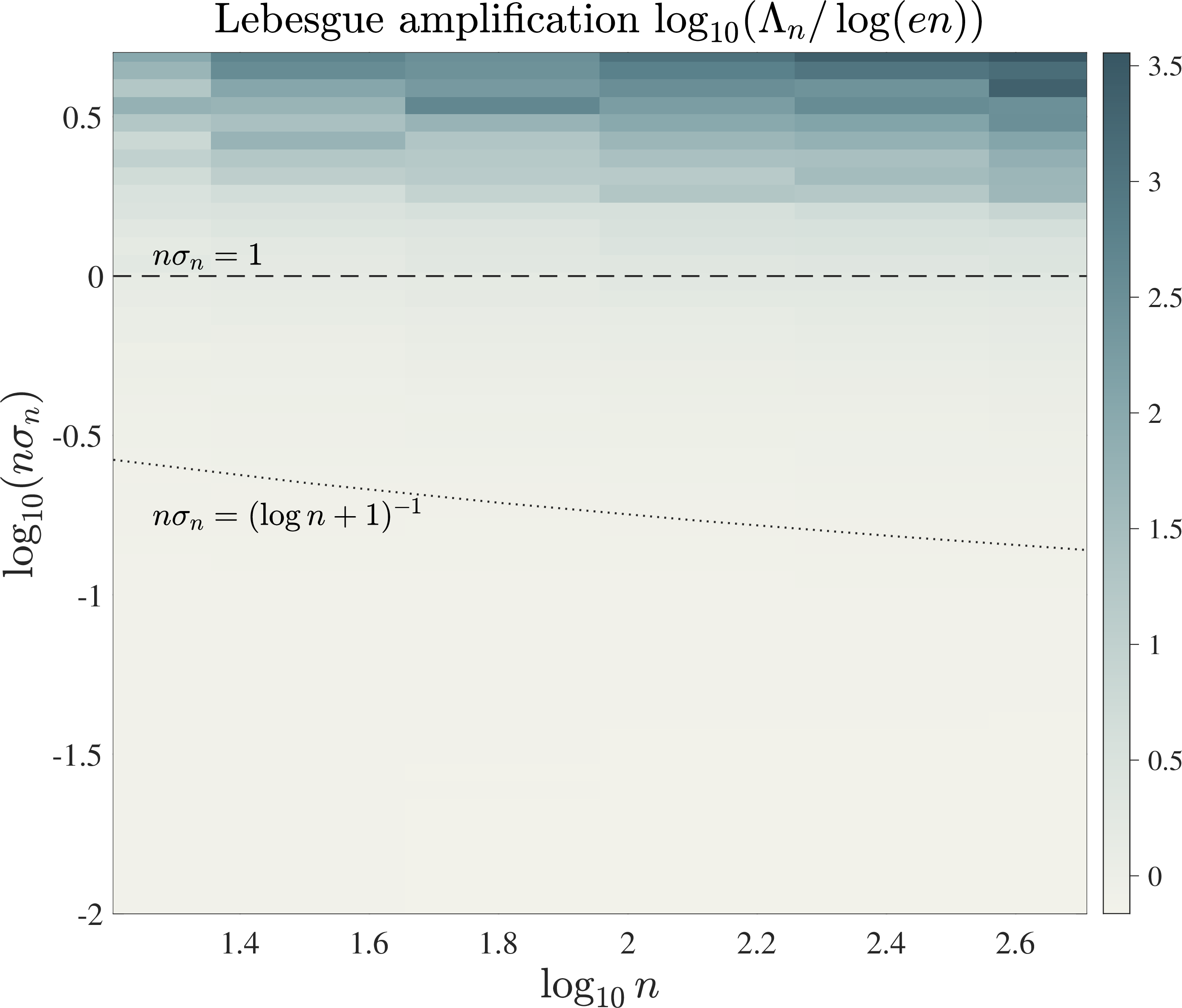
Figure 1 shows the effect of varying the mesh fraction \(n\sigma_n\). The plotted quantity is not \(\Lambda_n\) itself, but \(\Lambda_n/\log(en)\), so that values of order one correspond to Chebyshev scale growth. A stable region is visible for small \(n\sigma_n\), while larger mesh fractions lead to much stronger amplification. The natural mesh scale \(n\sigma_n=1\) is marked for orientation, but the numerics suggest a more subtle boundary: the transition layer is roughly parallel to the curve \[n\sigma_n=(\log n+1)^{-1}.\] This observation motivates the deterministic estimate proved in this paper. We do not claim that this curve is the exact probabilistic threshold for random perturbations. Rather, it identifies the small-constant scale at which a worst-case argument guarantees that the Lebesgue constant remains logarithmic.
Two related lines of work should be mentioned. Austin and Trefethen [4] studied trigonometric interpolation and quadrature on perturbed equispaced periodic grids, where fixed mesh-fraction perturbations can be allowed. The present paper concerns algebraic interpolation at Chebyshev–Lobatto points. The relevant geometry is no longer the periodic grid itself, but the cosine map from a uniform angular grid to the interval. The result is therefore local in the mesh fraction: we prove deterministic logarithmic stability for angular perturbations of size \(O((n\log n)^{-1})\), with a sufficiently small constant.
The work is also related to stability inequalities for norming sets, especially those of Piazzon and Vianello [5]. Their Markov-type framework gives a general perturbation principle for Lebesgue constants. For Chebyshev–Lobatto points, the angular parametrization improves the relevant one-dimensional scale: the usual Markov factor \(n^2\) in the physical variable is replaced by the trigonometric Bernstein factor \(n\) for \(p(\cos\theta)\). This distinction, and the relation between the two perturbation scales, is discussed after the main theorem.
The paper is organized as follows. Section 2 recalls the interpolation notation and the operator interpretation of the Lebesgue constant. Section 3 proves the deterministic stability estimate and gives a near-collision obstruction at the angular mesh scale. Section 4 translates the logarithmic stability bound into analytic interpolation estimates and a Runge-type interpretation. Section 5 records the corresponding consequence for pseudospectral differentiation, and Section 6 presents the numerical experiments.
2 Interpolation and Lebesgue constants↩︎
Let \(\mathcal{X}_n = \{x_0,\dots,x_n\} \subset [-1,1]\) be a set of distinct nodes and let \(\{f(x_j)\}_{j=0}^n\) be function values sampled on \(\mathcal{X}_n\). The Lagrange interpolation is defined by \[I_n f(x) = \sum_{j=0}^n f(x_j)\, \ell_j(x),\] where the Lagrange basis polynomials are given by \[\ell_j(x) = \prod_{\substack{k=0,\, k\neq j}}^n \frac{x-x_k}{x_j-x_k}, \qquad j=0,\dots,n.\] A key quantity controlling the stability of this interpolation is the Lebesgue function, \[\lambda_n(x) = \sum_{j=0}^n |\ell_j(x)|,\] whose maximum over \([-1,1]\) is the Lebesgue constant \[\label{equ:Lebesgue} \Lambda_n = \max_{x\in[-1,1]}\lambda_n(x).\tag{3}\] The Lebesgue constant \(\Lambda_n\) measures how much errors in the data \(f(x_j)\) are amplified in the interpolant. Indeed, the interpolation error satisfies the classical inequality \[\|f-I_n f\|_\infty \le (1+\Lambda_n)\, E_n(f),\] where \[E_n(f) = \inf_{p\in \mathbb{P}_n} \|f-p\|_\infty\] denotes the best uniform approximation error; see, e.g., [1]. Hence, the Lebesgue constant \(\Lambda_n\) quantifies the departure of the interpolation from the best uniform polynomial approximation.
3 Lebesgue constants under angular perturbations↩︎
In this section we prove a deterministic stability theorem for the Lebesgue constant under small angular perturbations of the Chebyshev–Lobatto points. The argument is based on a simple comparison between polynomial data sampled at the perturbed nodes and polynomial data sampled at the unperturbed Chebyshev–Lobatto nodes.
Recall that \[x_j^{(0)}=\cos\theta_j^{(0)}, \qquad \theta_j^{(0)}=\frac{j\pi}{n}, \qquad j=0,\ldots,n,\] denote unperturbed Chebyshev–Lobatto nodes and \[x_j=\cos\theta_j, \qquad \theta_j=\theta_j^{(0)}+\varepsilon_j, \qquad j=0,\ldots,n,\] are perturbed ones. We assume throughout this section that the perturbed nodes \(x_0,\ldots,x_n\) are distinct. Let \(\Lambda_n^{(0)}\) denote the Lebesgue constant of the Chebyshev–Lobatto points \(x_j^{(0)}\), and let \(\Lambda_n\) denote the Lebesgue constant of the perturbed points \(x_j\).
3.1 A logarithmic stability bound↩︎
We first consider an operator-norm characterization of the Lebesgue constant.
Lemma 1. For a set of distinct interpolation nodes \(\mathcal{X}_n=\{x_0,\ldots,x_n\}\subset[-1,1]\), let \[\Lambda(\mathcal{X}_n)=\max_{x\in[-1,1]}\sum_{j=0}^n |\ell_j(x)|\] denote the corresponding Lebesgue constant. Then \[\label{equ:characterization} \Lambda(\mathcal{X}_n) = \sup_{p\in\mathbb{P}_n,\, \max_{0\le j\le n}|p(x_j)|\le 1} \|p\|_{L^\infty[-1,1]}.\qquad{(2)}\]
For every \(p\in\mathbb{P}_n\), \[p(x)=\sum_{j=0}^n p(x_j)\ell_j(x),\] and therefore \[|p(x)| \le \max_{0\le j\le n}|p(x_j)| \sum_{j=0}^n |\ell_j(x)|.\]
Taking the maximum over \(x\in[-1,1]\) gives \[\|p\|_\infty \le \Lambda(\mathcal{X}_n)\max_{0\leq j\leq n}|p(x_j)|.\] Conversely, let \(x^*\in[-1,1]\) be a
point where the Lebesgue function attains its maximum, and define \[a_j=\operatorname{sgn}\ell_j(x^*),\qquad 0\le j\le n,\] with an arbitrary choice when \(\ell_j(x^*)=0\). Let \[p^*(x)=\sum_{j=0}^n a_j\ell_j(x).\] Then \(p^*\in\mathbb{P}_n\) and \[\max_{0\le j\le n}|p^*(x_j)|=\max_{0\le j\le n}|a_j|\le 1.\] Moreover, \[|p^*(x^*)| = \left|\sum_{j=0}^n a_j\ell_j(x^*)\right| = \sum_{j=0}^n |\ell_j(x^*)| = \Lambda(\mathcal{X}_n).\] Hence \[\sup_{p\in\mathbb{P}_n,\, \max_{0\le j\le n}|p(x_j)|\le 1}
\|p\|_{L^\infty[-1,1]} \ge \Lambda(\mathcal{X}_n).\] Together with the previous inequality, the desired characterization ?? follows. \(\square\)
Theorem 1 (Deterministic stability under angular perturbations). Assume that the perturbed nodes are distinct and that the angular perturbations are uniformly bounded by \[\max_{0\le j\le n}|\varepsilon_j|\le \sigma_n,\] where \(\sigma_n>0\) denotes the maximal magnitude of the perturbation in the angular variable. If the magnitude \(\sigma_n\) satisfies \[n\sigma_n\Lambda_n^{(0)}<1,\] then the Lebesgue constant of the perturbed nodes \(\{x_j\}_{j=0}^n\) satisfies \[\label{equ:mainestimate} \Lambda_n \le \frac{\Lambda_n^{(0)}}{1-n\sigma_n\Lambda_n^{(0)}}.\qquad{(3)}\]
Let \(p\in\mathbb{P}_n\) satisfy \[\max_{0\le j\le n}|p(x_j)|\le 1.\] We shall bound \(\|p\|_\infty\) in terms of the Lebesgue constant \(\Lambda_n^{(0)}\) of unperturbed nodes. Define \[q(\theta):=p(\cos\theta), \qquad \theta\in\mathbb{R}.\] Since \(p\) has degree at most \(n\), \(q\) is a trigonometric polynomial of degree at most \(n\). Hence Bernstein’s inequality for trigonometric polynomials gives \[\|q'\|_{L^\infty(\mathbb{R})} \le n\|q\|_{L^\infty(\mathbb{R})}.\] Since \(\|q\|_{L^\infty(\mathbb{R})} = \|p\|_{L^\infty[-1,1]}\), we obtain \[\|q'\|_{L^\infty(\mathbb{R})} \le n\|p\|_{L^\infty[-1,1]}.\] For each \(j=0,\ldots,n\), the mean value theorem gives \[\begin{align} |p(x_j^{(0)})| &=
|q(\theta_j^{(0)})| \le |q(\theta_j)| + |q(\theta_j^{(0)})-q(\theta_j)| \\ &\le |p(x_j)| + \|q'\|_{L^\infty[0,\pi]} |\theta_j^{(0)}-\theta_j| \\ &\le 1 + n\sigma_n \|p\|_{L^\infty[-1,1]}.
\end{align}\] Therefore \[\label{equ:previousestimate} \max_{0\le j\le n}|p(x_j^{(0)})| \le 1+n\sigma_n\|p\|_{L^\infty[-1,1]}.\tag{4}\] Since \(p\in\mathbb{P}_n\), it is exactly the polynomial interpolant of its values at the Chebyshev–Lobatto points. By the definition of \(\Lambda_n^{(0)}\) and Lemma 1, \[\|p\|_{L^\infty[-1,1]} \le \Lambda_n^{(0)} \max_{0\le j\le n}|p(x_j^{(0)})|.\] Combining this with the previous estimate 4 gives \[\|p\|_{L^\infty[-1,1]} \le \Lambda_n^{(0)} \left( 1+n\sigma_n\|p\|_{L^\infty[-1,1]} \right).\] Equivalently, \[\left(1-n\sigma_n\Lambda_n^{(0)}\right) \|p\|_{L^\infty[-1,1]} \le \Lambda_n^{(0)}.\] Since \(n\sigma_n\Lambda_n^{(0)}<1\), we obtain \[\|p\|_{L^\infty[-1,1]} \le
\frac{\Lambda_n^{(0)}}{1-n\sigma_n\Lambda_n^{(0)}}.\] This bound holds for every \(p\in\mathbb{P}_n\) satisfying \(\max_j|p(x_j)|\le1\). By the operator-norm characterization of the
Lebesgue constant in Lemma 1, the desired estimate ?? follows. \(\square\)
Theorem 2 (Explicit logarithmic stability regime). Let \[x_j=\cos\left(\frac{j\pi}{n}+\varepsilon_j\right), \qquad j=0,\ldots,n,\] be distinct perturbed Chebyshev–Lobatto nodes, with \(\varepsilon_0=\varepsilon_n=0\) and \(\max_j|\varepsilon_j|\le\sigma_n\). Let \(\eta\) be a constant satisfying \[0<\eta< \left(1+\frac{2}{\pi}\right)^{-1}\approx 0.611015,\] and assume that \[\label{equ:explicit-stability-assumption} n\sigma_n\left(\log n+1\right)\le \eta.\qquad{(4)}\] Then the Lebesgue constant \(\Lambda_n\) of the perturbed nodes satisfies \[\Lambda_n \le C_\eta\left(\log{n} +1\right),\] where \[C_\eta = \dfrac{1+\dfrac{2}{\pi}} {1-\left(1+\dfrac{2}{\pi}\right)\eta}.\] In particular, the perturbed points have logarithmically growing Lebesgue constants whenever \[n\sigma_n\log n\to0.\]
We use the explicit estimate \[\Lambda_n^{(0)} \le \frac{2}{\pi}\log(n+1)+1\] for the Chebyshev–Lobatto Lebesgue constant. Since \(n+1\le en\) and \(1\le
\log(en)\) for \(n\ge1\), we have \(\log(n+1)\le \log(en)\) and \[\Lambda_n^{(0)} \le \frac{2}{\pi}\log(en)+\log(en) =
\left(1+\frac{2}{\pi}\right)\left(\log{n} +1\right).\] It follows from the assumption ?? that \[n\sigma_n\Lambda_n^{(0)} \le \left(1+\frac{2}{\pi}\right)n\sigma_n(\log n +1) \le \left(1+\frac{2}{\pi}\right)\eta
<1.\] Hence the deterministic stability estimate ?? of Theorem 1 applies and gives \[\Lambda_n \le
\frac{\Lambda_n^{(0)}}{1-n\sigma_n\Lambda_n^{(0)}}.\] Using the two bounds above, we obtain \[\Lambda_n \le \frac{ \left(1+\frac{2}{\pi}\right)\log(en) }{ 1-\left(1+\frac{2}{\pi}\right)\eta }.\] Thus \[\Lambda_n \le C_\eta\log(en), \qquad C_\eta = \frac{1+\frac{2}{\pi}}{1-\left(1+\frac{2}{\pi}\right)\eta}.\] Finally, if \(n\sigma_n\log n\to0\), then for every fixed \[0<\eta<\left(1+\frac{2}{\pi}\right)^{-1},\] the condition \(n\sigma_n\log(en)\le\eta\) holds for all sufficiently large \(n\). Hence \(\Lambda_n=O(\log n)\). \(\square\)
Remark 1. Theorem 2 gives a deterministic stability regime. It does not claim to identify a sharp threshold for random perturbations. Rather, it shows that angular perturbations of size \[\sigma_n=o\!\left(\frac{1}{n\log n}\right)\] cannot destroy the logarithmic growth of the Chebyshev–Lobatto Lebesgue constant. The numerical experiments suggest that typical random perturbations may remain stable in a larger regime, but this sharper probabilistic question is separate from the deterministic estimate proved here.
Remark 2 (Angular versus \(x\)-variable perturbations). The scale in Theorem 2 should be interpreted in the angular variable. It is not the same as a uniform perturbation scale in the physical variable \(x\). This is the point at which the present result differs from the general norming-set perturbation principle of Piazzon and Vianello [5]. In that framework, stability is obtained from a Lebesgue constant and a Markov-type constant for the underlying polynomial space. On the interval, this uses the classical Markov inequality \[\|p'\|_\infty\le n^2\|p\|_\infty,\] and therefore gives, for the Chebyshev–Lobatto grid, perturbations satisfying \[\max_j |x_j-x_j^{(0)}| = O\!\left(\frac{1}{n^2\log n}\right)\] with a sufficiently small constant, because \(\Lambda_n^{(0)}=O(\log n)\). This is the usual interval scale obtained from a Markov-type perturbation argument.
By contrast, the angular parametrization gives \[x=\cos\theta, \qquad q(\theta)=p(\cos\theta),\] and therefore the trigonometric Bernstein inequality gives only a factor \(n\). Consequently, angular perturbations of size \[\sigma_n=O\!\left(\frac{1}{n\log n}\right)\] are covered when the implicit constant is sufficiently small. Thus the improvement is not a contradiction of the Markov–norming-set bound; it comes from measuring perturbations in the Chebyshev angular variable. In the \(x\)-variable such perturbations are nonuniform: they are of order \(O((n^2\log n)^{-1})\) near the endpoints and of order \(O((n\log n)^{-1})\) in the interior. This is the geometry one expects for perturbations that preserve the Chebyshev clustering.
3.2 An obstruction at the mesh scale↩︎
The preceding estimate gives a deterministic stability guarantee at the small-constant scale \[\sigma_n = O\!\left(\frac{1}{n\log n}\right).\] It is natural to ask whether this scale can be enlarged all the way to the angular mesh width \(h_n=\pi/n\). This is the first larger scale one would try, since \(h_n\) is the spacing of the unperturbed nodes in the angular variable. The following elementary construction shows that arbitrary perturbations at the mesh scale cannot preserve Chebyshev-type stability. The obstruction is a near collision of two neighbouring angular nodes.
Proposition 1 (A near-collision obstruction). Let \(h_n=\pi/n\), and let \(\tau_n\in(0,1/4)\). For every \(n\ge 4\), there exists a perturbed Chebyshev–Lobatto set \[x_j=\cos\theta_j,\qquad j=0,\ldots,n,\] with \[\max_{0\le j\le n}|\theta_j-jh_n|\le \frac{h_n}{2},\] such that its Lebesgue constant satisfies \[\Lambda_n \ge \frac{1}{\pi n\tau_n}.\] Consequently, by taking for example \[\tau_n=\frac{1}{n(\log n)^2},\] one obtains a sequence of angular perturbations of size \(O(1/n)\) for which \[\Lambda_n \ge \frac{1}{\pi}(\log n)^2.\] In particular, arbitrary mesh-scale angular perturbations are not covered by a logarithmic stability principle. They can lead to Lebesgue constants growing faster than \(\log n\).
Set \(h_n=\pi/n\), and choose \(m=\lfloor n/2\rfloor\). We perturb only the two neighbouring angular nodes \(m h_n\) and \((m+1)h_n\). Define \[\theta_m=\left(m+\frac{1}{2}\right)h_n-\tau_n h_n, \qquad \theta_{m+1}=\left(m+\frac{1}{2}\right)h_n+\tau_n h_n,\] and set \(\theta_j=jh_n\) for all \(j\ne m,m+1\). Then the angular perturbations satisfy \[|\theta_m-mh_n|=|\theta_{m+1}-(m+1)h_n| =\left(\frac{1}{2}-\tau_n\right)h_n \le \frac{h_n}{2},\] and all nodes are distinct.
Let \(x_j=\cos\theta_j\), and let \(p_n\in\mathbb{P}_n\) be the interpolation polynomial defined by the nodal values \[p_n(x_m)=1,\qquad p_n(x_{m+1})=-1,\qquad p_n(x_j)=0\quad (j\ne m,m+1).\] Thus \[\max_{0\le j\le n}|p_n(x_j)|\le 1.\] By the operator-norm characterization of the Lebesgue constant in Lemma 1, \[\Lambda_n\ge \|p_n\|_{L^\infty[-1,1]}.\]
On the other hand, by the mean value theorem, \[\|p_n'\|_{L^\infty[-1,1]} \ge \frac{|p_n(x_m)-p_n(x_{m+1})|}{|x_m-x_{m+1}|} = \frac{2}{|x_m-x_{m+1}|}.\] Markov’s inequality on \([-1,1]\) gives \[\|p_n'\|_{L^\infty[-1,1]} \le n^2 \|p_n\|_{L^\infty[-1,1]}.\] Therefore \[\|p_n\|_{L^\infty[-1,1]} \ge \frac{2}{n^2 |x_m-x_{m+1}|}.\] It
remains to estimate the distance between the two nearly colliding nodes. Since the cosine function is Lipschitz with constant one, \[|x_m-x_{m+1}| = |\cos\theta_m-\cos\theta_{m+1}| \le |\theta_m-\theta_{m+1}| = 2\tau_n h_n =
\frac{2\pi\tau_n}{n}.\] Hence \[\|p_n\|_{L^\infty[-1,1]} \ge \frac{2}{n^2(2\pi\tau_n/n)} = \frac{1}{\pi n\tau_n}.\] Since \(\Lambda_n\ge \|p_n\|_{L^\infty[-1,1]}\), the desired lower
bound follows. The choice \(\tau_n=1/(n(\log n)^2)\) gives \[\Lambda_n\ge \frac{1}{\pi}(\log n)^2,\] which is superlogarithmic. This completes the proof. \(\square\)
Remark 3. The construction is deliberately adversarial: it uses an almost collision of two neighbouring nodes. It therefore does not show that the deterministic scale \((n\log n)^{-1}\) is sharp. Rather, it shows that the stability result cannot be extended to arbitrary perturbations of order \(1/n\). The intermediate regime \[\frac{1}{n\log n}\ll \sigma_n \ll \frac{1}{n}\] remains a separate question, and the numerical phase diagrams below suggest that typical random perturbations may behave better than this worst-case near-collision example.
4 Analytic interpolation and Runge-type behaviour↩︎
For \(\rho>1\), let \(E_\rho\) denote the open Bernstein ellipse with foci \(\pm1\), whose boundary is the image of \(|w|=\rho\) under \(z=(w+w^{-1})/2\). If \(f\) is analytic in \(E_\rho\) and continuous on \(\overline{E}_\rho\), set \[M_\rho=\max_{z\in \overline{E}_\rho}|f(z)|.\] We shall use the standard Bernstein estimate \[\label{equ:bernstein-best-approximation} E_n(f) := \inf_{p\in\mathbb{P}_n}\|f-p\|_{L^\infty[-1,1]} \le \frac{2M_\rho}{\rho-1}\rho^{-n},\tag{5}\] see, for example, [1], [6].
Corollary 1 (Analytic interpolation at perturbed Chebyshev–Lobatto points). Let \(f\) be analytic in \(E_\rho\), \(\rho>1\), and continuous on \(\overline{E}_\rho\). For each \(n\), let \(I_n^\varepsilon f\) be the interpolant at distinct perturbed Chebyshev–Lobatto nodes satisfying \[x_j=\cos\left(\frac{j\pi}{n}+\varepsilon_j\right), \qquad \max_{0\le j\le n}|\varepsilon_j|\le \sigma_n .\] Assume that, for some fixed \(\eta\), \[n\sigma_n(\log n+1)\le \eta, \qquad 0<\eta<\left(1+\frac{2}{\pi}\right)^{-1}.\] Then \[\label{equ:analytic-interpolation-error} \|f-I_n^\varepsilon f\|_{L^\infty[-1,1]} \le \left(1+C_\eta\log(en)\right) \frac{2M_\rho}{\rho-1}\rho^{-n}.\qquad{(5)}\] In particular, \(I_n^\varepsilon f\to f\) uniformly on \([-1,1]\).
The Lebesgue inequality gives \[\|f-I_n^\varepsilon f\|_\infty \le (1+\Lambda_n)E_n(f).\] By Theorem 2,
\(\Lambda_n\le C_\eta\log(en)\). Together with 5 , this proves ?? . Since \(\log(en)\rho^{-n}\to0\), the asserted convergence follows.
\(\square\)
Corollary 2 (The Runge function under stable perturbations). Let \[f_R(x)=\frac{1}{1+25x^2}.\] Let \(I_n^\varepsilon f_R\) be defined as in Corollary 1. If \[n\sigma_n(\log n+1)\le \eta, \qquad 0<\eta<\left(1+\frac{2}{\pi}\right)^{-1},\] then, for every \[1<\rho<\rho_R, \qquad \rho_R=\frac{1}{5}+\sqrt{1+\frac{1}{25}},\] there is a constant \(M_\rho\) such that \[\|f_R-I_n^\varepsilon f_R\|_{L^\infty[-1,1]} \le \left(1+C_\eta\log(en)\right) \frac{2M_\rho}{\rho-1}\rho^{-n}.\] Consequently \(I_n^\varepsilon f_R\to f_R\) uniformly on \([-1,1]\). In this analytic setting, stable perturbed Chebyshev–Lobatto interpolation does not exhibit Runge-type divergence.
The singularities of \(f_R\) are at \(\pm i/5\). Hence \(f_R\) is analytic in \(E_\rho\) and continuous on \(\overline{E}_\rho\) for every \(1<\rho<\rho_R\). The result is Corollary 1. \(\square\)
For equally spaced interpolation, the corresponding Lebesgue constants grow exponentially; see [7], [8]. The preceding corollaries isolate the different mechanism here: the factor \(1+\Lambda_n\) is only logarithmic and cannot dominate the Bernstein decay \(\rho^{-n}\).
5 Pseudospectral differentiation↩︎
The preceding section shows that interpolation at the perturbed Chebyshev–Lobatto points remains spectrally accurate for analytic functions in the deterministic stability regime. We also record the corresponding consistency consequence for pseudospectral differentiation. The underlying mechanism is the same stability estimate in a differentiated form: a pseudospectral derivative is obtained by differentiating the interpolation polynomial, see, e.g., [9], and Markov’s inequality converts uniform stability of interpolation into stability of any fixed number of derivatives, at the cost of a polynomial factor in \(n\). This factor does not destroy the geometric decay supplied by analyticity in a Bernstein ellipse. Error behaviour for differentiated Chebyshev spectral approximations is also closely related to localization phenomena; see, e.g., [10].
Let \[x_j=\cos\left(\frac{j\pi}{n}+\varepsilon_j\right), \qquad j=0,\ldots,n,\] and let \(I_n^\varepsilon\) denote the interpolation operator at these perturbed nodes: \[I_n^\varepsilon f\in \mathbb{P}_n, \qquad I_n^\varepsilon f(x_j)=f(x_j), \qquad j=0,\ldots,n.\] If \(\ell_j^\varepsilon\) are the corresponding Lagrange basis polynomials, then \[I_n^\varepsilon f(x) = \sum_{j=0}^n f(x_j)\ell_j^\varepsilon(x),\] and the pseudospectral approximation of the \(m\)-th derivative is \[(I_n^\varepsilon f)^{(m)}(x) = \sum_{j=0}^n f(x_j)(\ell_j^\varepsilon)^{(m)}(x).\] In particular, evaluating this expression at the nodes gives the usual pseudospectral differentiation matrix \[D_{ij}^{(m),\varepsilon} = (\ell_j^\varepsilon)^{(m)}(x_i), \qquad 0\le i,j\le n.\]
Theorem 3 (Perturbed pseudospectral differentiation). Assume that the nodes are distinct and that \[\max_{0\le j\le n}|\varepsilon_j|\le \sigma_n .\] Suppose moreover that, for some fixed \(\eta\), \[n\sigma_n(\log n+1)\le \eta, \qquad 0<\eta<\left(1+\frac{2}{\pi}\right)^{-1}.\] Let \(f\) be analytic in the Bernstein ellipse \(E_\rho\), \(\rho>1\), and continuous on \(\overline{E}_\rho\). Set \[M_\rho=\max_{z\in\overline{E}_\rho}|f(z)|.\] Then, for every fixed integer \(m\ge1\), there exists a constant \(C_{\rho,m,\eta}>0\), independent of \(n\), such that \[\left\| f^{(m)}-(I_n^\varepsilon f)^{(m)} \right\|_\infty \le C_{\rho,m,\eta} M_\rho\, n^{2m}\log(en)\rho^{-n}.\] Consequently, \[\max_{0\le i\le n} \left| f^{(m)}(x_i) - \sum_{j=0}^n f(x_j)(\ell_j^\varepsilon)^{(m)}(x_i) \right| \le C_{\rho,m,\eta} M_\rho\, n^{2m}\log(en)\rho^{-n}.\] In particular, for each fixed derivative order \(m\), pseudospectral differentiation at the perturbed nodes is spectrally accurate.
The case \(m=0\) is exactly the interpolation estimate proved in Corollary 1. We therefore assume \(m\ge1\).
Let \(p_n\in \mathbb{P}_n\) be a polynomial approximant to \(f\) satisfying the standard Bernstein estimates \[\|f-p_n\|_\infty \le C_\rho M_\rho \rho^{-n},\] and, for the fixed integer \(m\), \[\|f^{(m)}-p_n^{(m)}\|_\infty \le C_{\rho,m}M_\rho n^{2m}\rho^{-n}.\] For example, \(p_n\) may be taken to be the truncated Chebyshev expansion of \(f\).
Since \(p_n\in \mathbb{P}_n\), interpolation is exact on \(p_n\): \[I_n^\varepsilon p_n=p_n.\] Therefore \[f-I_n^\varepsilon f = (f-p_n)-I_n^\varepsilon(f-p_n).\] Differentiating \(m\) times gives \[f^{(m)}-(I_n^\varepsilon f)^{(m)} = \bigl(f^{(m)}-p_n^{(m)}\bigr) - \bigl(I_n^\varepsilon(f-p_n)\bigr)^{(m)}.\] Hence \[\left\| f^{(m)}-(I_n^\varepsilon f)^{(m)} \right\|_\infty \le \|f^{(m)}-p_n^{(m)}\|_\infty + \left\| \bigl(I_n^\varepsilon(f-p_n)\bigr)^{(m)} \right\|_\infty .\]
The first term is already bounded by \[C_{\rho,m}M_\rho n^{2m}\rho^{-n}.\] For the second term, \(I_n^\varepsilon(f-p_n)\) is a polynomial of degree at most \(n\). By Markov’s inequality, for every \(r\in \mathbb{P}_n\), \[\|r^{(m)}\|_\infty \le C_m n^{2m}\|r\|_\infty .\] Applying this to \(I_n^\varepsilon(f-p_n)\), we obtain \[\left\| \bigl(I_n^\varepsilon(f-p_n)\bigr)^{(m)} \right\|_\infty \le C_m n^{2m} \|I_n^\varepsilon(f-p_n)\|_\infty.\]
The operator norm of the interpolation operator is the Lebesgue constant. Thus \[\|I_n^\varepsilon g\|_\infty \le \Lambda_n\|g\|_\infty .\] By Theorem 2, \(\Lambda_n\le C_\eta\log(en)\). Therefore \[\begin{align} \|I_n^\varepsilon(f-p_n)\|_\infty &\le \Lambda_n\|f-p_n\|_\infty \le C_\eta\log(en)\, C_\rho M_\rho\rho^{-n}. \end{align}\] Consequently, \[\left\| \bigl(I_n^\varepsilon(f-p_n)\bigr)^{(m)} \right\|_\infty \le C_{\rho,m,\eta} M_\rho n^{2m}\log(en)\rho^{-n}.\] Combining this estimate with the bound for \(\|f^{(m)}-p_n^{(m)}\|_\infty\) gives \[\left\| f^{(m)}-(I_n^\varepsilon f)^{(m)} \right\|_\infty \le C_{\rho,m,\eta} M_\rho n^{2m}\log(en)\rho^{-n}.\] This proves the continuous pseudospectral differentiation estimate.
Finally, evaluating the same estimate at the nodes \(x_i\) gives \[\max_{0\le i\le n} \left| f^{(m)}(x_i) - (I_n^\varepsilon f)^{(m)}(x_i) \right| \le C_{\rho,m,\eta} M_\rho
n^{2m}\log(en)\rho^{-n}.\] Since \[(I_n^\varepsilon f)^{(m)}(x_i) = \sum_{j=0}^n f(x_j)(\ell_j^\varepsilon)^{(m)}(x_i),\] this is exactly the differentiation-matrix estimate. \(\square\)
Remark 4. Theorem 3 concerns pseudospectral differentiation of a given analytic function. It should not be read as a complete convergence theorem for a pseudospectral collocation method applied to a differential equation. For a full collocation scheme, one also has to control the stability or invertibility of the resulting discrete differential operator. The result here is a consistency statement: in the deterministic stability regime, the perturbed interpolation grid itself does not destroy spectral accuracy of the differentiated interpolant.
6 Numerical experiments↩︎
We close with numerical experiments illustrating the preceding estimates.
6.1 Lebesgue constants and Lebesgue functions↩︎
We first examine the Lebesgue constants and Lebesgue functions of perturbed Chebyshev–Lobatto points. The random perturbations are generated in the angular variable, as in ?? , with \[\varepsilon_0=\varepsilon_n=0, \qquad \varepsilon_j\sim {\rm Unif}[-\sigma_n,\sigma_n], \qquad j=1,\ldots,n-1,\] for some scale \(\sigma_n\) to be specified in the following text. For each randomly generated node set, the nodes are sorted increasingly before the Lebesgue function is evaluated.
For the numerical evaluation we use the barycentric formula [11], not as an additional assumption but as a stable way of evaluating the same Lagrange interpolants and Lebesgue functions defined in Section 2. Thus the Lagrange basis polynomials need not be formed explicitly. If \[w_j=\prod_{k\ne j}(x_j-x_k)^{-1},\] then away from the nodes the Lebesgue function is computed as \[\lambda_n(x) =\sum_{j=0}^n|\ell_j(x)| = \frac{\displaystyle \sum_{j=0}^n \left|w_j/(x-x_j)\right|}{\displaystyle \left|\sum_{j=0}^n w_j/(x-x_j)\right|}.\] At the interpolation nodes we set \(\lambda_n(x_j)=1\). To avoid overflow in the weights, the magnitudes are formed logarithmically, \[\log |w_j| = -\sum_{k\ne j}\log |x_j-x_k|,\] and then shifted by their maximum before exponentiation. The signs alternate after sorting the nodes. The Lebesgue constant is then approximated by maximizing \(\lambda_n\) on a dense mixed grid consisting of a uniform grid in \(x\) and a uniform grid in the angular variable \(x=\cos\theta\). For the Lebesgue-function plots below, additional endpoint-refined grid points are included in order to resolve the large peaks of the equally spaced nodes near \(\pm1\).

Figure 2 compares perturbations at the scale \((n(\log n+1))^{-1}\), below it, at the angular mesh scale \(n^{-1}\), and above the mesh scale. The theorem gives logarithmic stability when \(n\sigma_n(\log n+1)\) is bounded by a sufficiently small constant. The plotted curve with \(\sigma_n=(n(\log n+1))^{-1}\) has constant one in this scale, so it is not covered by the explicit small-constant theorem, but it follows the unperturbed Chebyshev–Lobatto curve closely in this experiment. The slightly smaller scale \(n^{-1.2}\) also behaves in the same way. At the mesh scale \(n^{-1}\), the growth is still moderate but visibly larger. By contrast, the larger perturbation \(0.4n^{-0.8}\) produces much larger Lebesgue constants over the computed range. This is the numerical counterpart of the analytical message: sufficiently small angular perturbations preserve the Chebyshev mechanism, while larger perturbations can create substantial amplification.
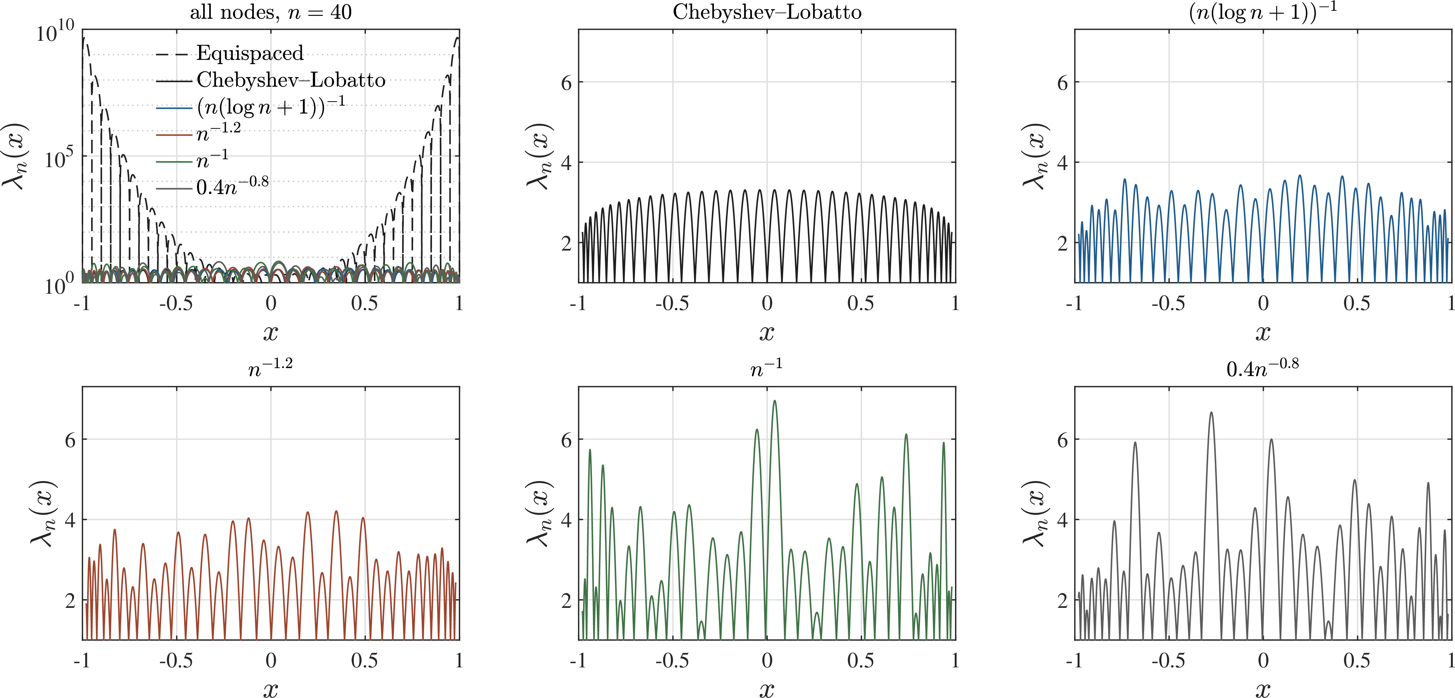
Figure 3 shows where the amplification measured by the Lebesgue constant occurs. For equally spaced nodes, the Lebesgue function develops large endpoint peaks, which is the familiar mechanism behind the instability of equally spaced interpolation. In contrast, the Chebyshev–Lobatto Lebesgue function is much flatter and remains on a logarithmic scale. The perturbations at and below the logarithmic stability scale have nearly the same profile as the unperturbed Chebyshev–Lobatto points. The larger \(0.4n^{-0.8}\) perturbation produces more pronounced peaks, consistent with the larger values of \(\Lambda_n\) in Figure 2. Thus the function-level plots support the same conclusion as the constants: the issue is not merely the size of the largest value, but the emergence of localized peaks in the Lebesgue function as the angular perturbations become larger.
6.2 Interpolants of the Runge function↩︎
The next experiment returns to the classical Runge function \[f(x)=\frac{1}{1+25x^2}.\] For each degree \(n\), we compare its polynomial interpolants on equally spaced nodes, on the Chebyshev–Lobatto nodes, and on one random perturbation of the Chebyshev–Lobatto nodes at the logarithmic scale. The perturbed nodes are again formed in the angular variable, \[x_j^\varepsilon = \cos\left(\frac{j\pi}{n}+\varepsilon_j\right), \qquad \varepsilon_0=\varepsilon_n=0, \qquad \varepsilon_j\sim {\rm Unif}\left[-\frac{1}{n(\log n+1)},\frac{1}{n(\log n+1)}\right].\] Thus the perturbation has the same asymptotic order as the deterministic scale, but with constant one; the explicit theorem requires a sufficiently small constant in this scale. The interpolants are evaluated on a dense uniform plotting grid using the barycentric formula with the same logarithmically scaled weights as above. For the equally spaced case, the usual explicit binomial form of the barycentric weights is used.
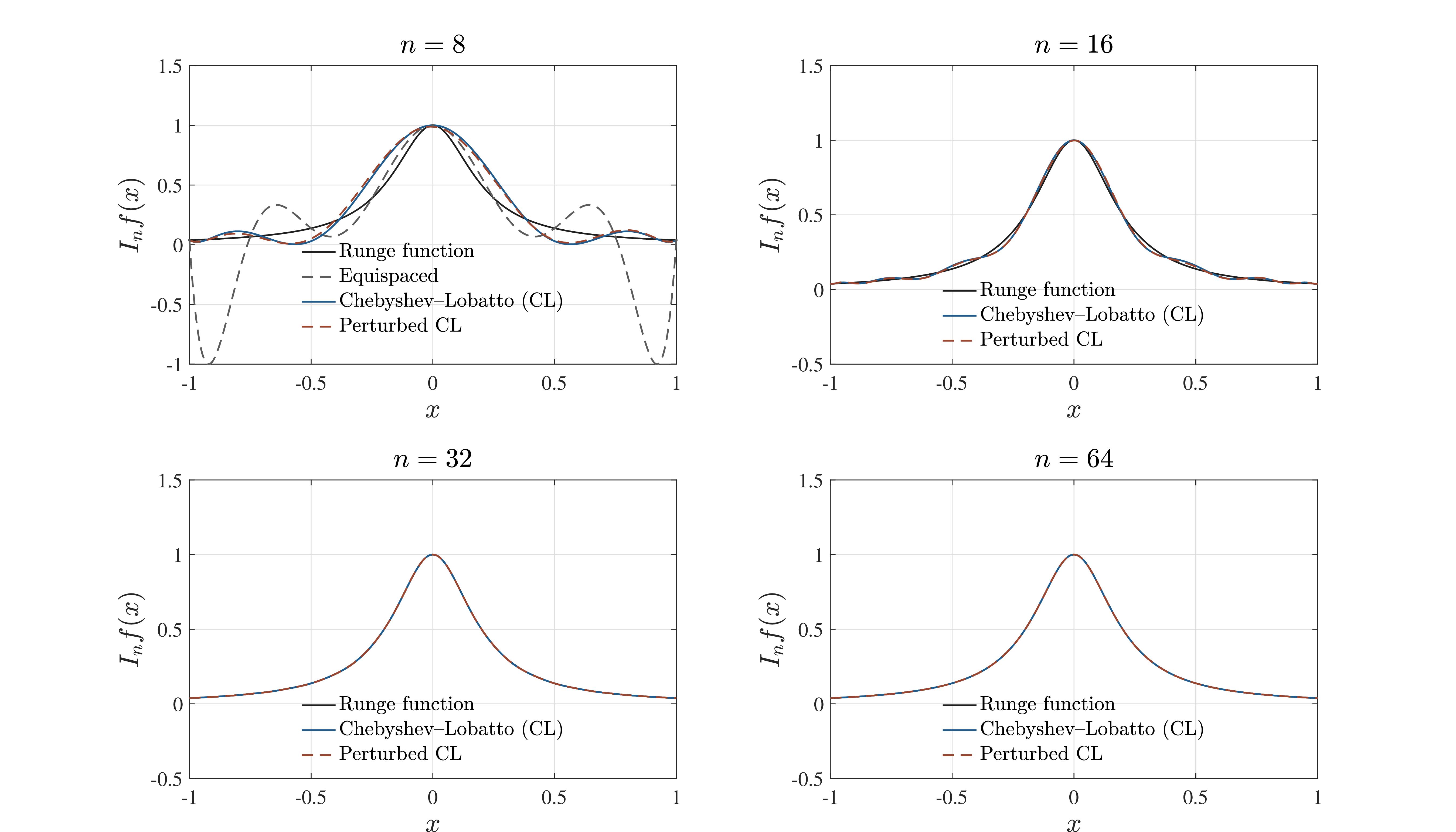
Figure 4 connects the Lebesgue-constant behaviour with the shape of the interpolating polynomials themselves. Equally spaced interpolation is vulnerable to the large endpoint peaks already visible in the Lebesgue function: even for the Runge function, whose singularities are fixed away from the real interval, the polynomial may develop large endpoint oscillations as \(n\) increases. The Chebyshev–Lobatto interpolants avoid this mechanism by placing many nodes near the endpoints. The stable perturbed Chebyshev–Lobatto interpolants are visually indistinguishable from the unperturbed ones at this scale, apart from small random changes in the curve. This is consistent with Corollary 1: the Bernstein-ellipse approximation error decays geometrically, and a logarithmically growing Lebesgue constant cannot overturn that decay. In this analytic setting, perturbations at this logarithmic scale therefore do not exhibit Runge-type divergence.
6.3 Differentiation errors↩︎
The last experiment illustrates the pseudospectral consequence discussed in Section 5. We take \[f(x)=e^x\sin(3x),\] so that \(f\), \(f'\), and \(f''\) are known explicitly. For the node set \(\mathcal{X}_n^\varepsilon=\{x_j^\varepsilon\}_{j=0}^n\), we compute the interpolant \(I_n^\varepsilon f\), the first differentiation matrix \[D_{ij}^{(1),\varepsilon} = \frac{w_j}{w_i(x_i-x_j)},\qquad i\ne j, \qquad D_{ii}^{(1),\varepsilon} = -\sum_{j\ne i}D_{ij}^{(1),\varepsilon},\] where \(w_j\) are the barycentric weights, and set \[D^{(2),\varepsilon}=(D^{(1),\varepsilon})^2.\] Table 1 reports the errors for \(m=0,1,2\). The interpolation error is evaluated on a dense uniform grid, while the derivative errors are evaluated at the interpolation nodes: \[\|f-I_n^\varepsilon f\|_\infty,\qquad \max_{x_i\in\mathcal{X}_n^\varepsilon} |f'(x_i)-(I_n^\varepsilon f)'(x_i)|,\] and \[\max_{x_i\in\mathcal{X}_n^\varepsilon} |f''(x_i)-(I_n^\varepsilon f)''(x_i)|.\] The random perturbations are again angular perturbations with \[\varepsilon_j\sim {\rm Unif}[-\sigma_n,\sigma_n], \qquad \varepsilon_0=\varepsilon_n=0,\] using the same four scales as in Figure 2. The random entries in the table are medians over eight independent perturbations; the Chebyshev–Lobatto row is deterministic.
| \(n\) | nodes | \(m=0\) | \(m=1\) | \(m=2\) |
|---|---|---|---|---|
| 32 | Chebyshev–Lobatto | \(1.89\times 10^{-15}\) | \(1.45\times 10^{-13}\) | \(4.14\times 10^{-11}\) |
| \((n(\log n+1))^{-1}\) | \(1.78\times 10^{-15}\) | \(1.22\times 10^{-13}\) | \(3.04\times 10^{-11}\) | |
| \(n^{-1.2}\) | \(2.33\times 10^{-15}\) | \(1.95\times 10^{-13}\) | \(2.89\times 10^{-11}\) | |
| \(n^{-1}\) | \(2.90\times 10^{-15}\) | \(2.10\times 10^{-13}\) | \(8.76\times 10^{-11}\) | |
| \(0.4n^{-0.8}\) | \(2.64\times 10^{-15}\) | \(1.49\times 10^{-13}\) | \(8.04\times 10^{-11}\) | |
| 64 | Chebyshev–Lobatto | \(4.44\times 10^{-15}\) | \(1.51\times 10^{-12}\) | \(2.64\times 10^{-9}\) |
| \((n(\log n+1))^{-1}\) | \(3.89\times 10^{-15}\) | \(8.18\times 10^{-13}\) | \(1.16\times 10^{-9}\) | |
| \(n^{-1.2}\) | \(4.94\times 10^{-15}\) | \(5.61\times 10^{-13}\) | \(1.07\times 10^{-9}\) | |
| \(n^{-1}\) | \(9.77\times 10^{-15}\) | \(7.13\times 10^{-13}\) | \(1.31\times 10^{-9}\) | |
| \(0.4n^{-0.8}\) | \(8.02\times 10^{-15}\) | \(6.45\times 10^{-13}\) | \(6.59\times 10^{-10}\) | |
| 128 | Chebyshev–Lobatto | \(7.11\times 10^{-15}\) | \(1.46\times 10^{-12}\) | \(1.00\times 10^{-8}\) |
| \((n(\log n+1))^{-1}\) | \(6.72\times 10^{-15}\) | \(1.81\times 10^{-12}\) | \(1.16\times 10^{-8}\) | |
| \(n^{-1.2}\) | \(6.99\times 10^{-15}\) | \(2.15\times 10^{-12}\) | \(1.49\times 10^{-8}\) | |
| \(n^{-1}\) | \(1.98\times 10^{-14}\) | \(2.91\times 10^{-12}\) | \(2.03\times 10^{-8}\) | |
| \(0.4n^{-0.8}\) | \(2.38\times 10^{-14}\) | \(3.53\times 10^{-12}\) | \(3.16\times 10^{-8}\) |
Table 1 is intended as a finite-precision illustration of Theorem 3. Passing from interpolation to one or two derivatives introduces the expected polynomial loss in \(n\), so the derivative errors are larger than the interpolation errors and eventually reflect roundoff and differentiation conditioning. The perturbation scale \(\sigma_n=(n(\log n+1))^{-1}\), which has the same asymptotic order as the deterministic stability scale, remains close to the unperturbed Chebyshev–Lobatto behaviour, while the larger perturbation \(0.4n^{-0.8}\) gives somewhat larger and less regular errors, consistent with the Lebesgue-constant behaviour in Figure 2.
It is not significant if, for some values of \(n\), a stable perturbed grid slightly outperforms the unperturbed Chebyshev–Lobatto grid. The theorem is a stability result, not an optimality statement for every fixed function and every finite degree. Chebyshev–Lobatto points give a near-minimal interpolation amplification mechanism in a uniform sense, but the actual error for a particular analytic function also depends on the alignment of the nodes with the oscillation and endpoint behaviour of that function. A small random angular perturbation may therefore improve the finite-\(n\) constant, even though the asymptotic mechanism and the order of stability remain the same. The relevant comparison is the envelope: stable perturbations stay close to the Chebyshev–Lobatto behaviour, whereas perturbations beyond the stable scale can produce noticeably larger and less predictable errors.
7 Concluding remarks↩︎
The results of this paper point to a simple organizing principle: for Chebyshev–Lobatto interpolation, perturbation stability is most naturally measured in the angular variable. In that variable the Chebyshev–Lobatto points form a uniform grid, and the trigonometric Bernstein inequality gives the factor \(n\) that drives the estimate. This is why the scale \(n\sigma_n(\log n+1)\lesssim 1\), with a sufficiently small constant, appears in the deterministic theorem. Once the Lebesgue constant remains logarithmic, analytic interpolation is governed by the balance between the logarithmic amplification of the interpolation operator and the geometric decay supplied by Bernstein ellipses. The numerical experiments suggest that typical random perturbations may remain stable beyond the present worst-case scale, but identifying such a probabilistic threshold is a different problem from the deterministic estimate proved here.
There are several natural directions in which this angular viewpoint might be tested. For Legendre points, the error behaviour of Chebyshev and Legendre approximation has been studied in detail [6], [12]–[14], but perturbation stability should require a geometry adapted to the Legendre distribution rather than the cosine parametrization used here. In two dimensions, Padua points provide an analogue of Chebyshev-like interpolation on the square, with near-optimal Lebesgue growth and a structure tied to Lissajous curves [15], [16]. Understanding perturbations of this two-dimensional angular structure is a natural open problem.
Finally, the same question can be asked for related approximation operators. For interpolatory quadrature on perturbed Chebyshev–Lobatto points, recomputed weights retain degree-\(n\) exactness and inherit error control from interpolation, whereas using unperturbed Clenshaw–Curtis weights at perturbed nodes generally destroys polynomial exactness. For hyperinterpolation [17], [18] and quadrature-based Galerkin schemes [19], the analogue of the Lebesgue constant is a discrete norm or Marcinkiewicz–Zygmund stability condition. These examples point to the same broader issue: the useful notion of perturbation is dictated by the sampling geometry and by the operator norm that controls the approximation process.