The natural extension of the \((-\beta)\)-transformation
June 22, 2026
Abstract
We give a concrete construction of a natural extension of \((-\beta)\)-transformation when \(\beta\) is greater than the golden mean. Our construction relies on its Markov diagram and the eigenvectors of the associated countable Markov shifts. Its positive recurrence can be shown by path counting using a special property of the diagram. Our down-to-earth construction elucidates the result of Bruin-Kalle [1] by examples.
1 Comparison between \(\beta\)- and \((-\beta)\)-transformations↩︎
Let \(\beta\) be a real number greater than \(1\) and \({\mathcal{A}}=\{0,1,\dots, \lfloor \beta \rfloor\}\). The \(\beta\)-transformation is an interval map \(T_\beta\) on \([0,1)\) defined by \[T_\beta:x \longmapsto \beta x -\left\lfloor \beta x\right\rfloor.\] By iterating this map \(T_\beta\), we obtain an expansion \[x=\sum_{i=1}^{\infty}\frac{d_i}{\beta^i}=(d_1d_2\dots d_i\cdots)_\beta,\] where \(d_i=d_i(x):=\lfloor \beta T_{\beta}^{i-1}(x)\rfloor\in {\mathcal{A}}\).
The \(\beta\)-expansion of \(x\) is denoted by \(d(x,\beta)=d_1(x) d_2(x) \cdots\). Define \[d^*(1,\beta) :=\lim_{x\nearrow 1} d(x,\beta)= b_1 b_2 \cdots\] in the topology of sequence space. It is well known that \(d^*(1,\beta)\) plays a crucial role in describing the dynamics of \(\beta\)-expansion. Parry [2] and Ito-Takahashi [3] showed that an infinite word \(x_1x_2\dots\in {\mathcal{A}}^{{\mathbb{N}}}\) is realized as \(d(x,\beta)\) for some \(x\in [0,1)\) if and only if \[x_nx_{n+1}\dots \ll d^*(1,\beta)\] for all \(n\in {\mathbb{N}}\). Here \(\ll\) is the lexicographic order. Parry [2] also gave a combinatorial characterization of \(d^*(1,\beta)\). In the notation of [3], Corollary 1 in [2] can be stated as follows: a sequence \((b_i)_{i\ge1}\in {\mathcal{A}}^{{\mathbb{N}}}\) arises as \(d^*(1,\beta)\) for some \(\beta>1\) if and only if \[\label{SelfBeta} b_nb_{n+1}b_{n+2}\dots \ll b_1b_{2}b_{3}\dots\tag{1}\] for all \(n\ge 1\). A natural extension of \(\beta\)-expansion is constructed in [4] and [5]. Let \[\begin{align} \mathcal{R}_{\beta,i}=\left[0, T_\beta^i(1)\right]\times \left[0, \frac{1}{\beta^i}\right] \end{align}\] for all \(i\ge 0\) and the underlying space \(\mathcal{H}_\beta\) is obtained by stacking \(\mathcal{R}_{\beta,i+1}\) on the top of \(\mathcal{R}_{\beta,i}\) for each \(i \ge 0\).
If \((x,y)\in\mathcal{R}_{\beta,i}\), let \(x=(d_1d_2\cdots)_{\beta}\), \(y=(\underbrace{0\cdots0}_{i}c_{i+1}c_{i+2}\cdots)_{\beta}\). Then, \[\begin{align} \label{NaturalBeta} \mathcal{T}_{\beta} (x,y):= \left(T_{\beta}x, y^*\right)\in \begin{aligned} \left\{ \begin{array}{ll} \displaystyle \mathcal{R}_{\beta,0}, \quad \text{if}~ d_1<b_{i+1}, \\ [5pt] \displaystyle \mathcal{R}_{\beta,i+1}, \quad \text{if} ~ d_1=b_{i+1}, \end{array} \right. \end{aligned} \end{align}\tag{2}\] where \[\begin{align} y^{*}= \begin{aligned} \left\{ \begin{array}{ll} \displaystyle \frac{b_1}{\beta}+\cdots+\frac{b_i}{\beta^i}+\frac{d_1}{\beta^{i+1}}+\frac{y}{\beta}=(b_1\cdots b_id_1c_{i+1}c_{i+2}\cdots)_\beta, \quad \text{if}~ d_1<b_{i+1}, \\ [10pt] \displaystyle \frac{y}{\beta}=(\underbrace{0\cdots0}_{i+1}c_{i+1}c_{i+2}\cdots)_\beta, \quad \text{if} ~ d_1=b_{i+1}. \end{array} \right. \end{aligned} \end{align}\]
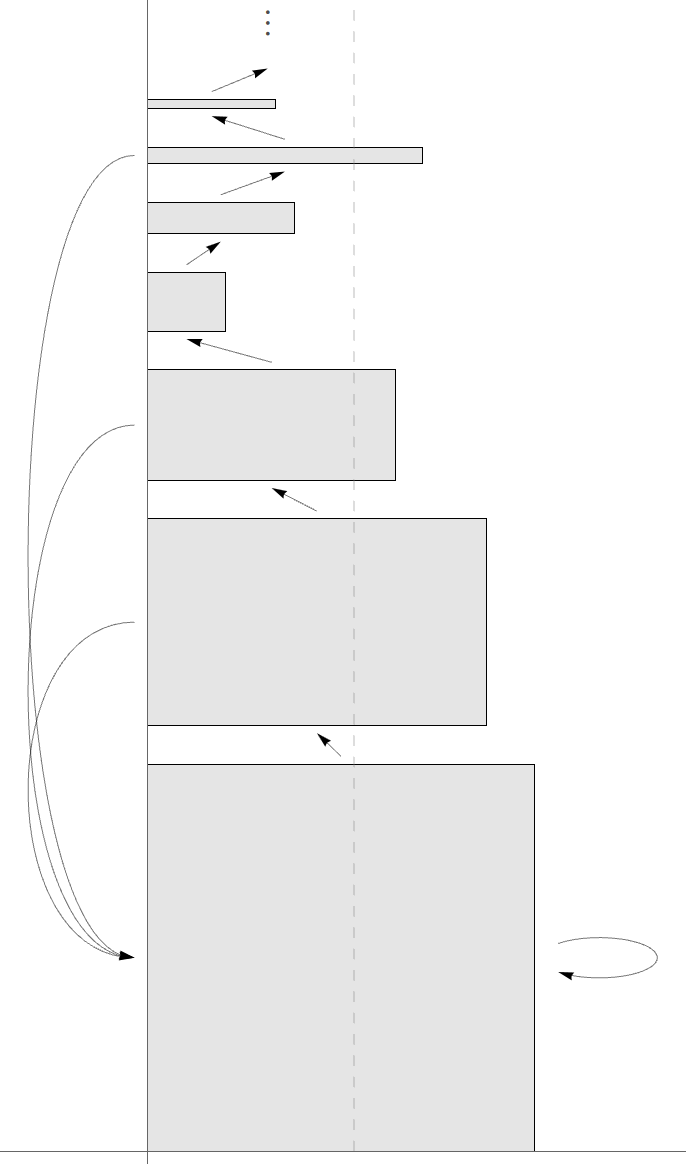
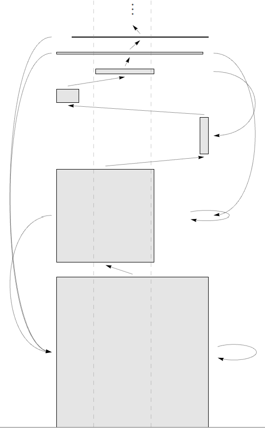
An example of this construction is depicted in 1. In this manner, the left sides of the rectangles are aligned, and the thicknesses of the rectangles are monotonically decreasing. Its absolutely continuous invariant density (not normalized) is given as a projection of the invariant measure (2-dimensional Lebesgue measure) of this natural extension: \[h_{\beta}(x)= \sum_{n\ge 0,~ x< T_{\beta}^n(1)}\frac{1}{\beta^n}.\]
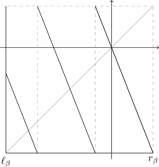
Ito-Sadahiro [6] denoted by \(I_\beta\) the half-open interval \([\ell_\beta, r_\beta)=[-\frac{\beta}{\beta+1}, \frac{1}{\beta+1})\) and defined \((-\beta)\)-transformation on \(I_\beta\) by \[T_{-\beta}:x \longmapsto-\beta x -\left\lfloor -\beta x-\ell_\beta\right\rfloor.\] Then, for each \(x\in I_\beta\), we have a \((-\beta)\)-expansion \(x=(d_1d_2\cdots)_{-\beta}\), where \[\begin{align} d_i=d_i(x):=\left\lfloor -\beta T_{-\beta}^{i-1}(x)-\ell_\beta \right\rfloor\in {\mathcal{A}}, \end{align}\] and \({\mathcal{A}}= \{0,1,\ldots, \lfloor \beta \rfloor \}\).
By applying the theorem of Li and Yorke [7], it is known that \(T_{-\beta}\) has a unique invariant measure absolutely continuous with respect to the Lebesgue measure and hence is ergodic. The following invariant density is due to [6]: \[\label{Density} h_{-\beta}(x)= \sum_{n\ge 0,~ T_{-\beta}^n(\ell_\beta)\le x}^{\infty}\frac{1}{(-\beta)^n}\tag{3}\] which is a solution of Kuzmin’s equation. However, its negative terms make it difficult to obtain a clear understanding of its dynamical system.
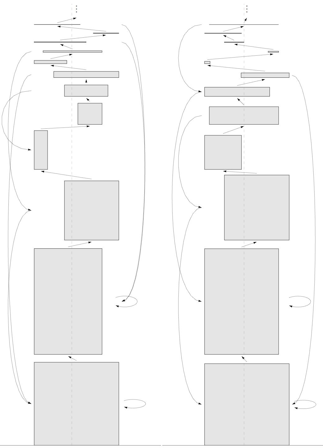
In this paper, we give a construction of the natural extension in this \((-\beta)\)-expansion only using positive terms, analogous to (2 ). Bruin-Kalle [1] gave a general approach to this type of piecewise linear maps, assuming several axioms. We revisit this in the setting of \((-\beta)\)-expansion and give a down-to-earth construction. The main technical difficulty is to show that the corresponding countable Markov shift is positive recurrent. We directly prove this in 2 by the path counting method using a particular property of the associated Markov diagram in Corollary 1. The reader will notice that the countable Markov shift gives a concrete way for construction, i.e., one can determine the measure rectangles explicitly as in 3, see 3. We observe that the natural extension is more involved than that of \(\beta\)-expansion: the thicknesses of the rectangles are not monotone decreasing, and the sides of the rectangles are not aligned, compare 1.
For \((x_i),(y_i)\in {\mathcal{A}}^{{\mathbb{N}}}\), we define \[(x_i)\prec (y_i)\] if \((-1)^i x_i < (-1)^i y_i\) at the smallest index \(i\) with \(x_i\neq y_i\), and \((x_i)\preceq (y_i)\) means \((x_i)=(y_i)\) or \((x_i)\prec (y_i)\). Let \(d(x,-\beta)=d_1d_2\dots\) by \(d_i=\lfloor -\beta T_{-\beta}^{i-1}(x)-\ell_{\beta} \rfloor\) for \(x\in [\ell_{\beta},r_{\beta})\). We set \(d^*(\ell_{\beta},-\beta)=\lim_{x\searrow \ell_{\beta}} d(x, -\beta)\) and \(d^*(r_{\beta},-\beta)=\lim_{x\nearrow r_{\beta}} d(x, -\beta)\). An infinite word \(x_1x_2\dots \in {\mathcal{A}}^{{\mathbb{N}}}\) is called admissible if it is in \(d([\ell_{\beta},r_{\beta}),-\beta)\). Then, Theorem 10 in [6] reads the sequence \((x_i)\in {\mathcal{A}}^{{\mathbb{N}}}\) is admissible if and only if \[\label{Adm} d(\ell_{\beta},-\beta)\preceq x_nx_{n+1}\dots \prec d^*(r_{\beta},-\beta)\tag{4}\] for all \(n\ge 1\). When \(\beta\) is fixed, this result characterizes infinite words in \({\mathcal{A}}^{{\mathbb{N}}}\) which appear as a \((-\beta)\)-expansion.
Let \[\eta:=\lim_{\beta\to 1+0} d(\ell_{\beta},-\beta)=100111001001001110011\cdots\] be the fixed point of the substitution \(\phi: 1\to 100,\;0\to 1\). As an analogy of (1 ), W. Steiner characterized the words in \({\mathcal{A}}^{{\mathbb{N}}}\) that appear as the expansion of \(\ell_{\beta}\), that is, the word of the form \(d(\ell_{\beta},-\beta)\) for some \(\beta>1\).
****Proposition** 1** (Steiner [8]). Let \((e_i)\in {\mathcal{A}}^{{\mathbb{N}}}\). There exists \(\beta>1\) that \(d(\ell_{\beta}, -\beta)=e_1e_2e_3\cdots\). if and only if it satisfies the following four conditions:
\(e_1e_2e_3\cdots \preceq e_{n}e_{n+1}e_{n+2}\cdots\) for \(n=1,2,3,\dots\),
\(\eta \succ e_1e_2\cdots\),
\(e_1e_2\cdots \not \in \{ e_1\cdots e_{k},e_1\cdots e_{k-1}(e_k-1)0\}^{\omega} \setminus \{(e_1\cdots e_k)^{\infty} \}\) for all \(k\ge 1\) that \(\eta\succ (e_1\cdots e_k)^{\infty}\),
\(e_1e_2\cdots \not \in \{ e_1\cdots e_{k}0, e_1\cdots e_{k-1}(e_{k}+1)\}^{\omega}\) for all \(k\ge 1\) that \(\eta\succ (e_1\cdots e_{k-1}(e_k+1))^{\infty}\).
Here, \(\{x,y\}^{\omega}\) denotes the set of infinite words generated by the concatenation of \(x\) and \(y\) in arbitrary order.
In section 2 and later, we have to use \(d^*(\ell_{\beta},-\beta)\) to construct the Markov diagram instead of \(d(\ell_{\beta},-\beta)\), because we use the corresponding symbolic dynamics on clopen sets. Fortunately, \[\label{OddPeriodcase} d^*(\ell_{\beta},-\beta)=d(\ell_{\beta},-\beta)\tag{5}\] holds for most values of \(\beta\), except when the orbit of \(\ell_{\beta}\) by \(T_{-\beta}\) forms an odd cycle. Indeed, if the orbit does not revisit \(\ell_{\beta}\), then the coding map is continuous at \(\ell_{\beta}\). Further, if it forms an even cycle, then it is right continuous at \(\ell_{\beta}\).
First, we discuss exceptional periodic expansions that cause some technical difficulty. We found such phenomena in 1 and 1. See also [6] and its remark afterward.
****Lemma** 1**. If the expansion is purely periodic: \(d(\ell_{\beta},-\beta)=(c_1c_2\dots c_{\ell})^{\infty}\), then \(c_{\ell}\ge 1\). Further, if \(\ell\) is odd, then we have \[d^*(\ell_{\beta},-\beta)=(c_1c_2\dots (c_{\ell}-1)0)^{\infty}\] and \[d^*(r_{\beta},-\beta)=(0c_1c_2\dots (c_{\ell}-1))^{\infty}\] and the set of sequence \((x_i)\in {\mathcal{A}}^{{\mathbb{N}}}\) which satisfies (4 ) but does not satisfy \[d^*(\ell_{\beta},-\beta)\preceq x_nx_{n+1}\dots \prec d^*(r_{\beta},-\beta)\] is countable. Such elements have the suffix \((c_1c_2\dots c_{\ell})^\infty\).
Proof. If \(d(\ell_{\beta},-\beta)=(c_1c_2\dots c_{\ell-1}0)^{\infty}\), then \(d(T_{-\beta}^{\ell-1}(\ell_{\beta}),-\beta)=(0c_1c_2\dots c_{\ell-1})^{\infty}\) which implies the contradiction \(T_{-\beta}^{\ell-1}(\ell_{\beta})=r_{\beta}\), since \(\ell_{\beta}=(-\beta)r_{\beta}\). If \(d(\ell_{\beta},-\beta)=(c_1c_2\dots c_{\ell})^{\infty}\), then \(T_{-\beta}^{\ell}(\ell_{\beta})=\ell_{\beta}\). If \(\ell\) is odd, then \(T_{-\beta}^{\ell}\) is right discontinuous at discontinuity points and we have \(d^*(\ell_{\beta},-\beta)= \lim_{\varepsilon\downarrow 0}d(\ell_{\beta}+\varepsilon,-\beta)= (c_1c_2\dots (c_{\ell}-1) 0)^{\infty}\) since \(\ell_{\beta}=(-\beta)r_{\beta}\) implies \(\lim_{\varepsilon\downarrow 0} T_{-\beta}(r_{\beta}-\varepsilon)=\ell_{\beta}\). We also have \(d^*(r_{\beta},-\beta)=\lim_{\varepsilon\downarrow 0}d(r_{\beta}-\varepsilon,-\beta)= (0c_1c_2\dots (c_{\ell}-1))^{\infty}\).
For the last statement, let \((x_i)\) be a sequence satisfying this condition. Then if \(x_nx_{n+1}\dots x_{n+\ell-1}= c_1\dots c_{\ell}\), then \(x_{n+\ell} \ge c_1\) implies \(x_{n+\ell}=c_1\). We also have \(c_2\le x_{n+\ell+1}\le c_2\) which implies \(x_{n+\ell+1}=c_2\). Repeating this, we see that \(x_nx_{n+1}\dots = (c_1c_2\dots c_{\ell})^{\infty}\). ◻
****Example** 1**. Let \((e_i)=\sum_{k=1}^{\infty} 1^k0^k=10110011100011110000\dots\). Since the prefix \(101\) appears only once, we can easily see that conditions of 1 are satisfied. There exists \(\beta\approx 1.80266\) and we see that \(d(\ell_{\beta},-\beta)=(e_i)_{i\ge0}\).
One can also show that \(\beta\) is transcendental. Indeed, \[\begin{align} -\frac{\beta}{1+\beta}&= \sum_{i=1}^{\infty} \frac{e_i}{(-\beta)^i}= \sum_{k=1}^{\infty} \frac{1}{(-\beta)^{k^2-k+1}}\frac{1-1/(-\beta)^{k}}{1-1/(-\beta)}\\ &=\frac{-1/\beta+(-1/\beta)^{3/4}\theta_{2}(-1/\beta)+ \theta_{3}(-1/\beta)/\beta}{2(1+1/\beta)} \end{align}\] where \(\theta_2,\theta_3\) are the elliptic theta null values: \[\theta_2(q)=\sum_{n\in {\mathbb{Z}}} q^{(n+1/2)^2}, \qquad \theta_3(q)=\sum_{n\in {\mathbb{Z}}} q^{n^2}\] with \(|q|<1\). By the algebraic independence result of theta null values, \(\beta\) cannot be algebraic, see Theorem 4 of [9] and [10]. For \(d\ge2\), \(\sum_{k=1}^{\infty}d^k(d-1)^k\cdots1^k0^k\) does not satisfy Condition 1.
****Example** 2**. Let \(\psi\) be a substitution defined by \(1\to 101\) and \(0\to 1\). We claim that the fixed point \[w:=(e_i)=\lim_{n\to \infty}\psi^n(1)=101 110110110111011011101\dots\] satisfies Conditions 1 and 2. We introduce a \({\mathbb{Z}}/2{\mathbb{Z}}\)-extension \(\overline{\psi}\): \[1\mapsto 101,\quad 0\mapsto \overline{1}, \quad \overline{1}\mapsto \overline{1}\overline{0}\overline{1}, \quad \overline{0}\mapsto 1.\] Here, the letter \(1\) is in the odd position, and \(\overline{1}\) is in the even position. Similarly \(0\) is in the even position and \(\overline{0}\) is in the odd position. \[\overline{w}:= \lim_{n\to \infty}\overline{\psi}^n(1)=101\overline{1}101\overline{1}\overline{0}\overline{1}101\overline{1}101\overline{1}\overline{0}\overline{1}1\overline{1}\overline{0}\overline{1}\dots\] In other words, the overline indicates that the letter \(\overline{1}\) (resp. \(\overline{0}\)) can not be replaced with \(0\) (resp. \(1\)) by Condition 1. Therefore \[\label{forbidden} 1010, 10111010, 101110111, 1011101100, 10111011011010, \dots\qquad{(1)}\] are forbidden by Condition 1. To prove the claim, we show that these words never appear as a factor of \(w\). By construction, \(00\), \(010\) are forbidden in \(w\) and \(0\overline{1}\), \(\overline{1}0\) are forbidden in \(\overline{w}\), in particular, the first \(1010\) does not appear. If a factor in (?? ) appears in \(w\), then it contains either one of the above forbidden words, or it must have a preimage of \(\phi\) which forms a shorter forbidden word in (?? ). This gives a contradiction, and we have established the claim.
Since \(00\) is a forbidden word and \(e_k=1\), Condition 3 of 1 is fulfilled. Similarly, Condition 4 is valid, since \(e_k=0\). Therefore, Proposition 1 guarantees that we have \(w=d(\ell_{\beta},-\beta)\) with a unique \(\beta \approx 1.875305172\).
2 Hofbauer’s Markov Diagram↩︎
In this section, we recall piecewise monotone maps on the unit interval \([0,1]\) (of course, it can also be \([\ell_{\beta}, r_{\beta}]\)) and their Markov diagrams.
****Definition** 1** (piecewise monotone map). We call \(T:[0,1]\to[0,1]\) a piecewise monotone map if there exist disjoint intervals \(I_0,\cdots, I_k\subset [0,1]\) with the partition points \(c_0=0<c_1< \ldots < c_{k+1}=1\) satisfying the following conditions:
\([0,1]=\displaystyle \bigcup_{j=0}^k I_j\),
\(T|_{I_j}\) is continuous and strictly monotone,
\(\displaystyle \bigcup_{n=1}^{\infty}T^{-n}\left([0,1]\setminus \bigcup_{j=0}^k Int(I_j)\right)\) is dense in \([0,1]\).
Let \[\label{clopenset} X_{T}:=\bigcap_{n=1}^{\infty}T^{-n}\left(\bigcup_{j=0}^k Int(I_j)\right),\tag{6}\] and define the coding map \(\Psi:X_T\to \Sigma_k^{+}=\{0,1,2,\dots,k\}^{\mathbb{N}}\) by \(\Psi(x)=j_1j_2\cdots\), where \(j_i\) is the index with \(T^{i-1}(x)\in I_{j_i}\). Set \[\Sigma_T^{+}=\{{\boldsymbol{x}}=x_1x_2\cdots\in \Sigma_k^{+}\mid a^{x_m}\preceq \sigma^{m-1}({\boldsymbol{x}})=x_{m}x_{m+1}\cdots\preceq b^{x_m} ~ for anym \in \mathbb{N} \},\] where \(\sigma\) is a shift transformation and \[\begin{align} a^{j}=\lim_{x\in I_j, ~x\searrow c_{j}}\Psi(x), \quad b^{j}=\lim_{x\in I_{j}, ~x\nearrow c_{j+1}}\Psi(x). \end{align}\]
Then, \(\Psi\) is injective, and the following diagram is commutative. It is surjective except for a countable set [11]: \[\begin{CD} {X_T} @>{T}>> {X_T} \\ @V{\Psi}VV @V{\Psi}VV \\ {\Sigma_{T}^{+}} @>{\sigma}>> {\Sigma_{T}^{+}} \end{CD}\]
Here, we denote \(\Psi(I_{w_1} \cap T^{-1}(I_{w_2}) \cap \cdots\cap T^{-n+1}(I_{w_n}) \cap X_T)\) by \([w_1w_2\cdots w_n]\) for \(n \in \mathbb{N}\) and \(w_1w_w \cdots w_n \in \{0,1,\ldots,k \}^\mathbb{N}\).
We now define the Markov diagram of Hofbauer, which is a countable directed graph whose vertex set is \(\Psi(X_{T})\).
****Definition** 2** (Hofbauer’s Markov Diagram). Let \(X\subset \{0,1,2,\dots, k\}^{\mathbb{N}}\) and \(C, D\subset X\). We denote \(C \rightarrow D\) if there exists \(i\in\{0,1,2,\dots, k\}\) such that \(D=\sigma(C)\cap [i]\not=\emptyset\). Define \(\mathcal{D}_i\) inductively as follows: \[\begin{align} \mathcal{D}_0:&=\{[0],[1],[2],\dots, [k]\}\\ \mathcal{D}_n:&=\{D \mid \exists C\in \mathcal{D}_{n-1}~ s.t.~ C\rightarrow D \} \quad \text{for~} n\in\mathbb{N}. \end{align}\] Set \(\mathcal{D}_X=\bigcup_{n=0}^{\infty}\mathcal{D}_n\). The pair \((\mathcal{D}_X,\rightarrow)\) is called Hofbauer’s Markov diagram.
When \(C \to D\), there exists unique \(i \in \{0,1,\ldots, k\}\) such that \(D \subset [i]\), and we label the arrow from \(C\) to \(D\) as \(i\) and write \(C \xrightarrow{i} D\). We consider the set of infinite paths on Hofbauer’s Markov diagram \((\mathcal{D}_X, \rightarrow)\): \[\Sigma_{\mathcal{D}_X}^+ := \{ (D_i)_{i \in \mathbb{N}} \in \mathcal{D}_X^{\mathbb{N}} \mid D_{i} \rightarrow D_{i+1}for anyn \in \mathbb{N}\},\] and define \(\Phi^+: \Sigma_{\mathcal{D}_X}^+ \to \{1,2,\ldots,k\}^\mathbb{N}\) by \(\Phi((D_i)_{i \in \mathbb{N}}) = (e_i)_{i \in \mathbb{N}}\) for \((D_i)_{i \in \mathbb{N}} \in \mathcal{D}_X^{\mathbb{N}}\) with \(D_i \xrightarrow{e_i} D_{i+1}\). Then \(\Sigma_T^+ = \Phi^+( \Sigma_{\mathcal{D}_X}^+)\) (See [12]).
For the original definition and study on Hofbauer’s Markov diagram, we can see [11], [13], and [14]. In particular, [12] includes the case of the decreasing map \(T\), and [1] provides several examples of towers for \(\beta\)-transformation and \((-\beta)\)-transformation.
Before starting the case of \((-\beta)\)-transformation \(T_{-\beta}\), let us recall the case of \(\beta\)-transformation \(T_\beta\). It is known that the Markov diagram is obtained in the following way by using the expansion \(d^*(1,\beta)= b_1 b_2 \cdots\) of 1.
The cylinders \([0],\dots,[b_1-1]\) work in the same way and merge into a single state \(0\). The cylinder \([b_1\dots b_{n-1}]\) corresponds to the state \(n\) for \(n\ge 1\).
The vertex set of the Markov diagram is \(\mathbb{N} \cup \{0\}\), and there exists an uparrow from the state \(n\) to the state \(n+1\) labeled by \(b_{n+1}\) and downarrows from the state \(n\) to the state \(0\) labeled by \(0,1,\ldots,b_{n+1}-1\) for \(n \in \mathbb{N} \cup \{0\}\) (See 4).

From now on, we study the case of (\(-\beta\))-transformation. Let \(d^{*}(\ell_{\beta}, -\beta)=b_1b_2\cdots\). Further, let the partition points \(c_0=r_\beta >c_1> \ldots >c_{b_1+1}=\ell_\beta\) be \(c_i=r_\beta-i/\beta\) for \(i \in \{0,1,\ldots,b_1\}\) and \(I_0 =(c_1,c_0], I_1=(c_2,c_1], I_2=(c_3,c_2],\ldots, I_{b_1}=[c_{b_1+1}, c_{b_1}]\).
The (\(-\beta)\)-transformation \(T_{-\beta}\) is a piecewise monotone map, and we can do the same as in the case of the map on \([0,1]\).
For brevity, we write \(T_{-\beta}^{n-1} (\ell_{\beta}^+) \in I_{b_n}\), to mean that \(T_{-\beta}^{n-1}(\ell_{\beta}+\varepsilon)\in I_{b_n}\) for all sufficiently small \(\varepsilon>0\).
By the definition of \(T_{-\beta}\), we have \(b_2<b_1\). Since \(\overline{\Psi^{-1}(\sigma([i]))}=[\ell_{\beta},r_{\beta}]=\cup_{j=0}^{b_1} \overline{I_j}\) for \(i\not=b_1\), \([i]\xrightarrow{j} [j]\) for \(i \in\{0,1,\dots,b_1-1\}\) and \(j \in\{0,1,\dots,b_1\}\). Since \(T_{-\beta}(\ell_{\beta}^+) \in I_{b_2}\) and \(\overline{\Psi^{-1}(\sigma([b_1]))}=[\ell_{\beta},T_{-\beta}(\ell_{\beta}^+)]=\cup_{j=b_2+1}^{b_1}\overline{I_j} \cup [c_{b_2+1},T_{-\beta}(\ell_{\beta}^+)]\), \[\begin{array}{l} [b_1]\xrightarrow{j} [j] \quad \quadforj\in\{b_2+1,\dots,b_1-1\},\\ [10pt] [b_1] \xrightarrow{b_1}[b_1],\\ [10pt] [b_1]\xrightarrow{b_2} \sigma([b_1])\cap[b_2]=\sigma([b_1b_2])=\Psi([c_{b_2+1}, T_{-\beta}(\ell_{\beta}^{+}))\cap X_T). \end{array}\] Similarly, since \(T_{-\beta}^2(\ell_{\beta}^+) \in I_{b_3}\) and \(\overline{\Psi^{-1}(\sigma^2([b_1b_2]))}=[T_{-\beta}^2(\ell_\beta^+),r_\beta]=\cup_{j=0}^{b_3-1}\overline{I_j} \cup [T_{-\beta}^2(\ell_\beta^+),c_{b_3}]\), \[\begin{array}{l} \sigma[b_1b_2] \xrightarrow{j} [j] \quad \quadforj \in\{0,1,\dots,b_3-1\},\\ [10pt] \sigma[b_1b_2] \xrightarrow{b_3} \sigma^2[b_1b_2b_3], \end{array},\] and we can see \[\begin{align} &\mathcal{D}_{1}\setminus \mathcal{D}_0=\{\sigma([b_1b_2])\},~ \mathcal{D}_{2}\setminus (\mathcal{D}_0\cup \mathcal{D}_1)=\{\sigma^2([b_1b_2b_3])\}, \cdots. \end{align}\] In the case of a \((-\beta)\)-transformation, there is only one non-full part such that \[\mathcal{D}_{n}\setminus \bigcup_{i=0}^{n-1}\mathcal{D}_i=\{\sigma^n([b_1b_2\cdots b_{n+1}])\}.\] 5 gives a figure of Hofbauer’s Markov diagram. In fact, by letting the state \(0\) of the diagram given by 5 denote the collection of \([0], [1], \ldots, [b_1-1]\) and the state \(n\) for \(n\in \mathbb{N}\) denote \(\sigma^{n-1}([b_1 b_2 \cdots b_{n}])\), this diagram becomes Hofbauer’s Markov diagram.

In the above discussion, the interval \(\overline{\Psi^{-1}(\sigma^n([b_1b_2\cdots b_n]))}\) and its endpoint \(T_{-\beta}^m(\ell_\beta^+)\) greatly help in finding edges from the state \(n\) in Hofbauer’s Markov diagram. We wish to continue this discussion using a realization as a tower. Let \(R_0=[\ell_\beta,r_\beta]\) and \(R_n=\overline{\Psi^{-1}(\sigma^n([b_1b_2\cdots b_n]))}\) for \(n \in \mathbb{N}\), and stack these intervals vertically to geometrically realize Hofbauer’s Markov diagram as in 6. Later, we will see in Theorem 3 that the exact locations and lengths of these intervals correspond to the shape of the right eigenvector of the incidence matrix of the Markov diagram. In what follows, we construct Hofbauer’s Markov diagram by using its tower realization depicted in 6.
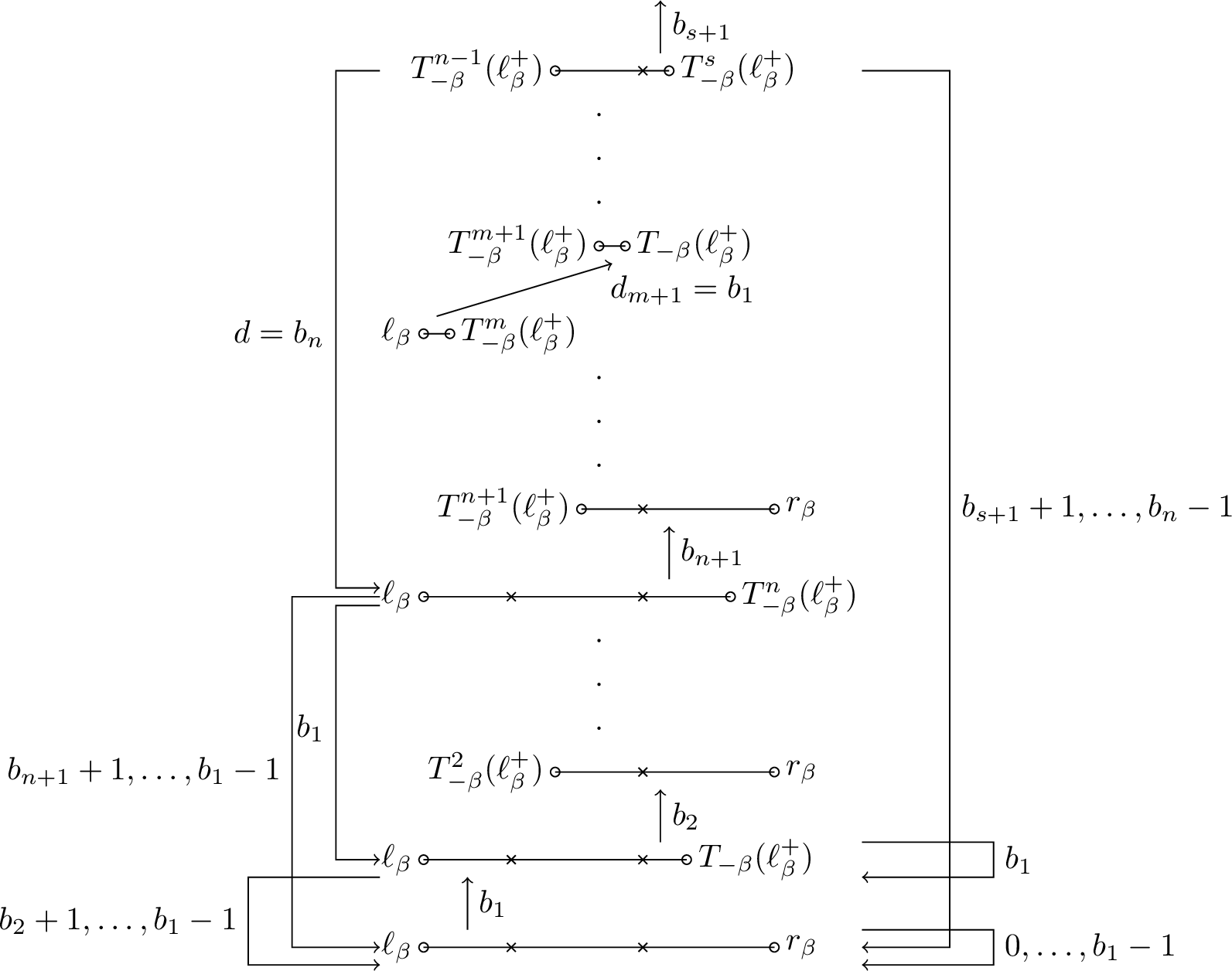
The Markov diagram is constructed level by level from the bottom for \(m=0,1,2,\ldots\). In this process, there are two cases, namely Case I and Case II, as described below. For each case, we examine how the edges from the \(m\)-th floor are drawn.
Case I: \(m\) is even, or \(m\) is odd and \(T_{-\beta}^{m}(\ell_{\beta}^+) \notin I_{b_1}\).
In this case, we have \[\begin{align}
\label{R95m} R_{m}=
\begin{aligned}
\left\{
\begin{array}{ll}
\displaystyle [\ell_\beta,T^{m}(\ell_{\beta}^{+})]
=\bigcup_{j=b_{m+1}+1}^{b_1}\overline{I_j}
\cup [c_{b_{m+1}+1},T^m_{-\beta}(\ell_{\beta}^+)],
\quad m: odd, \\
[10pt]
\displaystyle [T^{m}_{-\beta}(\ell_{\beta}^{+}),r_\beta]
=[T_{-\beta}^m(\ell_\beta^+),c_{b_{m+1}}] \cup \bigcup_{j=0}^{b_{m+1}-1}\overline{I_j},
\quad m: even
\end{array} \right.
\end{aligned}.
\end{align}\tag{7}\] Therefore, from the \(m\)-th floor there exists one uparrow to the \((m+1)\)-th floor labeled by \(b_{m+1}\). And there
exist downarrows to the \(0\)-th floor labeled by \(0,1,\ldots,b_{m+1}-1\) when \(m\) is even, or downarrows to the \(0\)-th
floor labeled by \(b_{m+1}+1, b_{m+1}+2,\ldots, b_1 -1\) and one downarrow to the 1st floor labeled by \(b_1\) when \(m\) is odd and \(T_{-\beta}^{m}(\ell_{\beta}^+) \notin I_{b_1}\).
Case II: \(m\) is odd and \(T_{-\beta}^{m}(\ell_{\beta}^+) \in I_{b_1}\).
In this case, \[\begin{align}
\label{R95m43a} R_{m+a}= \begin{aligned}
\left\{
\begin{array}{ll}
\displaystyle [T^{m+a}_{-\beta}(\ell_{\beta}^{+}),T^{a}(\ell_{\beta}^{+})], \quad a:odd, \\
[10pt]
\displaystyle [T^{a}(\ell_{\beta}^{+}), T^{m+a}_{-\beta}(\ell_{\beta}^{+})], \quad a:even,
\end{array} \right.
\end{aligned}
\end{align}\tag{8}\] and \(R_{m+a} \subset \overline{I_{b_a}}\) for some \(a=0,1,\cdots\). Since \(T_{-\beta}\) is expanding, there exists the
first index \(a\ge 1\) that \(R_{m+a}\) contains some of the partition points \(\{c_1, c_2, \ldots,c_{b_1} \}\). We denote this index \(a\) by \(n-1\). Then \(b_{m+1}=b_1, b_{m+2}=b_2, \ldots,b_{m+n-1}=b_{n-1}\) and \(b_{m+n} \ne b_{n}\) and
\[\begin{align} \label{R95m43n} R_{m+(n-1)}= \begin{aligned} \left\{ \begin{array}{ll} \displaystyle [T^{n-1}_{-\beta}(\ell_{\beta}^+),c_{b_{n}}] \cup \bigcup_{j=b_{m+n}+1}^{b_{n}-1} \overline{I_j} \cup [c_{b_{m+n}+1},T^{m+n-1}_{-\beta}(\ell_{\beta}^+)], \quad n: odd, \\ [13pt] \displaystyle [T^{m+n-1}_{-\beta}(\ell_{\beta}^+),c_{b_{m+n}}] \cup \bigcup_{j=b_{n}+1}^{b_{m+n}-1}\overline{I_j} \cup [c_{b_{n}+1},T^{n-1}_{-\beta}(\ell_{\beta}^+)], \quad n: even. \end{array} \right. \end{aligned} \end{align}\tag{9}\]
Therefore, for \(a \in \{0,1,\ldots, n-2\}\), there is no arrow from the \((m+a)\)-th floor to any lower floor, and there exists only one uparrow to the \((m+a+1)\)-th floor labeled by \(b_{m+a+1}\). From \((m+n-1)\)-th floor, there exists one uparrow to the \((m+n)\)-th floor labeled by \(b_{m+n}\), and there exists downarrows to the \(0\)-th floor labeled by \(b_{m+n}+1, b_{m+n}+2, \ldots, b_{n}-1\) when \(n\) is odd, or downarrows to the \(0\)-th floor labeled by \(b_{n}+1, b_{n}+2, \ldots, b_{m+n}-1\), when \(n\) is even. Note that \(R_m \subset \overline{I_{b_1}}\) and \(R_{m+a} \subset R_a\) for \(a \in \{1,2,\ldots,n-1\}\). Since \([T^{n-1}_{-\beta}(\ell_{\beta}^+), c_{b_{n}}]\subset R_{n-1}\) when \(n\) is odd or \([c_{b_{n}+1}, T^{n-1}_{-\beta}(\ell_{\beta}^+)] \subset R_{n-1}\) when \(n\) is even, there is one downarrow to the \(n\)-th floor labeled by \(b_{n}\) (In 5 and 6, we denote \(s:=m+n-1\)).
Moreover, we can see \(R_{n}=[\ell_\beta, T^{n}(\ell_\beta^+)]\) when \(n\) is odd or \(R_{n}=[T^{n}(\ell_\beta^+),r_\beta]\) when \(n\) is even. For \(a=1,2,\ldots,n-1\), \(R_n \ne R_{m+a}\), thus \(n \le m\).
Summarizing these discussions, Hofbauer’s Markov Diagram is given by the following rule:
****Theorem** 1** (How to construct the Markov diagram). Put \(d^*(\ell_{\beta},-\beta)=b_1b_2\dots .\) Let the collection of the cylinders \([0],[1],\ldots,[b_1-1]\) be the state
\(0\) and \(\sigma^{n-1}([b_1b_2\cdots b_n])\) the state \(n\) for \(n \in \mathbb{N}\). The edges of Hofbauer’s Markov
diagram are given by the following way:
There are self-loops and uparrows in the diagram as shown below. \[\begin{array}{l}
0 \xrightarrow{i} 0 \quad \quad \quadfori \in\{0,1,\dots,b_1-1\},\\
[10pt]
1 \xrightarrow{b_1} 1,\\
[10pt]
m \xrightarrow{b_{m+1}} m+1 \quad \quadform \in \mathbb{N} \cup \{0\}.
\end{array}\]
We draw downarrows by the following infinite algorithm starting from the state \(m\mapsto 1\).
\((*)\) Unless \(b_{m+1}=b_1\) with some odd number \(m\), draw downarrows as follows: \[\begin{array}{ll} m \xrightarrow{i} 0 \quad \quadfori \in \{0,1,\dots,b_{m+1}-1\} & m : even,\\ [10pt] \begin{align} &m \xrightarrow{i} 0 \quad \quadfori \in \{ b_{m+1}+1, b_{m+1}+2, \ldots,b_1-1\},\\ &m \xrightarrow{b_1} 1 \end{align} \qquad & m: odd. \end{array}\] Then we move to the next state \(m\mapsto m+1\) and return to \((*)\).
In the case where \(b_{m+1}=b_1, b_{m+2}=b_2, \ldots,b_{m+n-1}=b_{n-1}\) and \(b_{m+n} \ne b_{n}\) with some odd number \(m\) and \(n \le m\),
Draw downarrows from the state \(s:=m+n-1\) as follows: \[s \xrightarrow{b_{n}} n,\] and \[\begin{array}{ll} s \xrightarrow{i} 0 \quad \quadfori \in \{b_{n}+1, b_{n}+2, \ldots, b_{s+1}-1\} & n,s : even,\\ [10pt] s \xrightarrow{i} 0 \quad \quadfori \in \{b_{s+1}+1, b_{s+1}+2, \ldots, b_{n}-1\} & n,s: odd. \end{array}\] Then we move to the next state \(m\mapsto s+1\) and return to \((*)\).
****Remark** 1**. In the last part of the above proof of 1, we could directly see that the case where \(m\) is odd and \(n>m\) cannot occur, since the corresponding interval would be away from \(\ell_{\beta}\) and \(r_{\beta}\) and leads to a contradiction, if such a case exists. This can be shown in the following way as well. Since \(b_{m+a}=b_a\) for \(a=1,2,\dots,m\), by applying the same discussion as the last part of the proof of Lemma 1, the expansion is purely periodic of period \((b_1\dots b_m)^{\infty}\). But \(d^*(\ell_{\beta},-\beta)\) can not be in this form by Lemma 1. See 5 for the construction of the exceptional cases for (5 ).
We denote the countable incidence matrix of the Markov diagram by \(A_{-\beta}\).
In the Markov diagram in 1, we call \(i-j+1\) the defect of a downarrow \(i\rightarrow j\) with \(j\le i\).
****Corollary** 1**. The defects of the arrows \(i\rightarrow j\) with \(0<j\le i\) are distinct positive integers.
Proof. By 1, such a self-loop and downarrows have a form \(s \xrightarrow{b_{n}} n\) and \(s-n+1=m\), where \(m\) is the state of the Markov diagram that we visit by the above algorithm. ◻
This property will be used in the proof of 2, which is the clue to the construction of our natural extension.
3 Perron–Frobenius Theorem for Countable Markov Shifts↩︎
To prove the main theorem, we recall the Perron–Frobenius theorem described in [15] associated with the countable infinite matrix \({A}\) with non-negative entries.
We say such a matrix is irreducible if for every pair of indices \(i\) and \(j\), there is \(n\) with \(({A}^n)_{ij}>0\). Equivalently, the matrix is irreducible when its incidence graph is strongly connected.
Fix an index \(i\) and let \(p(i)=\gcd\{n\ge 1 \mid ({A}^n)_{ii} >0\}\). This is the period of the index \(i\). When \({A}\) is irreducible and the period of every index is the same, that is called the period of \({A}\). As before, a matrix with period one is said to be aperiodic. Note that \(({A})_{00}>0\) implies \({A}\) is aperiodic.
We will define three generating functions. For any pair of indices \(i\) and \(j\), we define \[\begin{align} a_{ij}(0)=\delta_{ij}, \quad a_{ij}(1)={A}_{ij}, \quad a_{ij}(n)=({A}^n)_{ij}. \end{align}\] The first generating function is defined by \[\begin{align} H_{ij}(z)=\sum_{n=0}^{\infty}a_{ij}(n)z^n. \end{align}\] For the next type of generating functions, we define coefficients inductively. Let \[\begin{align} \ell_{ij}(0)=0, \quad \ell_{ij}(1)=a_{ij}(1), \quad \ell_{ij}(n+1)=\sum_{r\not=i}\ell_{ir}(n)a_{rj}(1). \end{align}\] The coefficient \(\ell_{ij}(n)\) is the sum of the weights of the paths that go from \(i\) to \(j\) in \(n\) steps without returning to \(i\) at any time prior to \(n\). Define the functions \[\begin{align} L_{ij}(z)=\sum_{n=1}^{\infty}\ell_{ij}(n)z^n. \end{align}\]
Similarly, define coefficients \[\begin{align} r_{ij}(0)=0, \quad r_{ij}(1)=a_{ij}(1), \quad r_{ij}(n+1)=\sum_{r\not=j}a_{ir}(1)r_{rj}(n). \end{align}\] The coefficient \(r_{ij}(n)\) represents the sum of the weights of the paths that go from \(i\) to \(j\) in \(n\) steps without hitting \(j\) at any time prior to \(n\). Define the functions \[\begin{align} R_{ij}(z)=\sum_{n=1}^{\infty}r_{ij}(n)z^n. \end{align}\]
We define \(\lambda\) to be the Perron value of \({A}\). The irreducibility of \({A}\) implies \(\displaystyle \lambda=\lim_{n\rightarrow \infty}\sqrt[n]{({A}^n)_{ij}}\) (c.f. [15]). The matrix \({A}\) is recurrent if \(H_{ii}(1/\lambda)=\infty\). The recurrent matrix \({A}\) is said to be positive recurrent if \[\begin{align} \sum_{n=1}^{\infty}n\frac{\ell_{ii}(n)}{\lambda^n}<\infty, \end{align}\] and it is said to be null recurrent if \(\sum_{n=1}^{\infty}n\ell_{ii}(n)/\lambda^n=\infty\).
****Proposition** 2** (Generalized Perron-Frobenius Theorem, [15]). Suppose \({A}\) is a countable nonnegative
matrix. Further, suppose it is irreducible, aperiodic, and recurrent. Then there exists a finite Perron value \(\lambda>0\) such that:
\((a)\) \(\displaystyle \lambda=\lim_{n\rightarrow \infty}\sqrt[n]{({A}^n)_{ij}}\) for any pair of indices \(i\) and \(j\),
so that \(1/\lambda\) is the radius of convergence of the power series \(\displaystyle H_{ij}(z)=\sum_{n=0}^{\infty}a_{ij}(n)z^n\),
\((b)\) \(\lambda\) has strictly positive left and right eigenvectors,
\((c)\) the eigenvectors are unique up to constant multiples,
\((d)\) let \(\ell, r\) be the left and right eigenvectors for \(\lambda\) then \(\ell\cdot r<\infty\) if and only if
\({A}\) is positive recurrent,
\((e)\) if \(0\le S\le {A}\) and \(\beta\) is the Perron value for \(S\) then \(\beta\le\lambda\), if \(S\) is recurrent then there is equality if and only if \(S={A}\),
\((f)\) \(\displaystyle \lim_{n\rightarrow \infty}{A}^n/\lambda^n={\boldsymbol{0}}\) if \({A}\) is null recurrent, and \(\displaystyle \lim_{n\rightarrow \infty}{A}^n/\lambda^n=r \ell\), normalized so that \(\ell \cdot r=1\), if \({A}\) is positive recurrent.
From here, we list up the lemmas (including the lemmas of the Generalized Perron-Frobenius Theorem) necessary to prove the main theorem.
****Lemma** 2** ([15]). Suppose \({A}\) is a countable, nonnegative matrix. Further, suppose it is irreducible and aperiodic. Then \[\begin{align} H_{ii}(z)=\frac{1}{1-L_{ii}(z)}=\frac{1}{1-R_{ii}(z)}, \quad |z|<\frac{1}{\lambda}. \end{align}\]
****Lemma** 3** ([15]). Suppose \({A}\) is a countable, nonnegative, irreducible, and aperiodic matrix.
Then
\((i)\) either every \(H_{ij}(1/\lambda)\) is finite or every \(H_{ij}(1/\lambda)\) is infinite, and
\((ii)\) either every \(L_{ii}(1/\lambda)\) is less than one or every \(L_{ii}(1/\lambda)\) is equal to one.
We define the following vectors. For each \(i, j\), define a row and column vector \[\begin{align} \ell^{(i)}=(L_{i0}(1/\lambda), L_{i1}(1/\lambda), \dots, L_{ij}(1/\lambda), \dots), \quad r^{(j)}= \left( \begin{array}{c} R_{0j}(1/\lambda) \\ R_{1j}(1/\lambda) \\ \vdots \\ R_{ij}(1/\lambda) \\ \vdots \end{array} \right). \end{align}\]
By the following Lemma, these vectors are exactly the left and right eigenvectors, respectively.
****Lemma** 4** ([15]). Let \({A}\) be a countable, nonnegative, irreducible, aperiodic, and recurrent matrix. Then \[\begin{align} \ell^{(i)}{A}=\lambda\ell^{(i)}, ~ {A}r^{(i)}=\lambda r^{(i)} \quad\text{for all i}. \end{align}\]
****Proposition** 3** (Finite Approximation Theorem, [15]). Let \(A\) be a countable, infinite, non-negative matrix. Assume \(A\) is irreducible, aperiodic, and recurrent.
If \(\lambda\) is the Perron value for \(A\), \[\lambda = \sup\{\lambda(A'): A'is a finite, irreducible and aperiodic submatrix of A \},\] where \(\lambda (A') is the Perron value of the finite matrix A'\).
Let \(\ell\) and \(r\) be the left and right eigenvectors of \(A\) for the Perron value \(\lambda\), normalized so that for some index \(i\), \(\ell_i=r_i=1\). Let \(\{A_n\}\) be an increasing family of finite irreducible, aperiodic submatrices of \(A\) that converge to \(A\). Let \(\ell^{(n)}\), \(r^{(n)}\) be the left and right eigenvectors corresponding to their Perron values, normalized so that \(\ell_i^{(n)}=r_i^{(n)}=1\). Then \(\lim \ell_j^{(n)}=\ell_j\) and \(\lim r_j^{(n)}=r_j\) for all \(j\) in the index set.
In the \(\beta\)-expansion case, the countable incidence matrix of the Markov diagram given in 4 is \[\begin{align} {A}= \left( \begin{array}{ccccc} b_1 & 1 & & \\ b_2 & & 1 & \\ b_3 & & & \ddots\\ \vdots & & & \end{array} \right), \end{align}\] and the left and right eigenvectors corresponding to the eigenvalue \(\beta\) can be written explicitly as \[\begin{align} \ell^{(0)}=(1, 1/\beta, 1/\beta^2, \dots, 1/\beta^i, \dots), \quad r^{(0)}= \left( \begin{array}{c} 1 \\ T_{\beta}(1) \\ \vdots \\ T_{\beta}^i(1) \\ \vdots \end{array} \right). \end{align}\]
We see that the \(i\)-th entries of \(\ell^{(0)}\) and \(r^{(0)}\) give the width and height of the rectangle \(\mathcal{R}_{\beta,i}\).
****Lemma** 5** ([15]). Either \(L'_{ii}(1/\lambda)=\sum_{n=1}^{\infty}n\ell_{ii}(n)/\lambda^{n-1}\) is finite for all i and j, or it is infinite for all i and j.
We define the mean recurrence weight \(\mu(i)\) as \[\begin{align} \mu(i)=\frac{1}{\lambda}L'_{ii}(1/\lambda). \end{align}\]
****Lemma** 6** ([15]). If \({A}\) is positive recurrent, then \(\ell^{(i)}\cdot r^{(i)}=\mu(i)\).
We define a new quantity \(\varrho(i)\) as \[\begin{align} \varrho(i)=\limsup{\sqrt[n]{\ell_{ii}(n)}}. \end{align}\] Clearly, \(\varrho(i)\le \lambda\).
****Lemma** 7** ([15]). If \({A}\) is a matrix where \(\varrho(i)<\lambda\) for some state \(i\), then \({A}\) is positive recurrent.
4 The Natural Extension↩︎
By 2, the adjacency matrix \(A_{-\beta}\) of Hofbauer’s Markov Diagram in 5, 6 is given by \[\begin{align} \label{A95beta} {A}_{-\beta}= \bordermatrix{ & 0 & 1 & 2 & \cdots & n & n+1 & \cdots & m+a+1 & \cdots & s+1 & \cdots \cr 0 & b_1 & 1 & & & & & & & &\cr 1 & b_1-b_2-1 & 1 & 1 & & & & & & & &\cr \vdots & & & & \ddots & & & & & & \cr n & i & 0/1 & & & & 1 & & & & &\cr \vdots & & & & & & & \ddots & & & & \cr m+a & & & & & & & & 1 & & & \cr \vdots & & & & & & & & & \ddots & & \cr s & j & & & & 1 & & & & & 1 &\cr \vdots & & & & & & & & & & &\ddots \cr}, \end{align}\tag{10}\]
where the \((i, j)\) entry \(a_{ij}\) of the matrix \(A_{-\beta}\) is the number of the edges from the state \(i\) to the state \(j\) for \(i,j\ge 0\).
****Proposition** 4**. For \(\beta> (1+\sqrt{5})/2\), \({A}_{-\beta}\) is irreducible, aperiodic, and recurrent. Furthermore, the Perron value of \({A}_{-\beta}\) is \(\beta\).
The same assertion holds for \(1<\beta\le (1+\sqrt{5})/2\), if we properly restrict \(A_{-\beta}\) to its irreducible component, reflecting the support of the absolutely continuous invariant measure of \(T_{-\beta}\).
Proof. Since the map \(T_{-\beta}\) has a unique invariant measure that is equivalent to the Lebesgue measure, for any interval \(I, J \subset [\ell_\beta,r_\beta)\), there exists \(n\), \[\begin{align} \mu\left(T_{-\beta}^{-n}(I)\cap J\right)>0. \end{align}\] This implies that every state can be reached from every other state. Hence \({A}_{-\beta}\) is irreducible. Also, since \(({A}_{-\beta})_{00}>0\), \({A}_{-\beta}\) is aperiodic. By the definition of the map \(T_{-\beta}\), every interval is expanded by a factor of \(\beta\), and subdivided by the discontinuity points. When a subdivided interval becomes full, it is sent back to the unit interval. Counting such intervals yields \[\begin{align} L_{00}\left(\frac{1}{\beta}\right)=\sum_{n=1}^{\infty}\frac{\ell_{00}(n)}{\beta^n}=1. \end{align}\] Thus, by 2 and 3, \({A}_{-\beta}\) is recurrent, the radius of convergence of \(H_{ii}(z)\) is \(1/\beta\), and the Perron value of \({A}_{-\beta}\) is \(\beta\). ◻
For a finite set \({\mathcal{A}}\), we denote by \({\mathcal{A}}^*\) the monoid generated by concatenation over \({\mathcal{A}}\) which has the identity; namely the empty word.
****Lemma** 8**. Let \(W\) be a non-empty set of positive integers. Let \(s_W(k)\) be the cardinality of words in \(W^*\) whose arithmetic sum of letters is equal to \(k\). Then \[s_W(k)=\sum_{j\in W} s_W(k-j).\] holds for \(k\ge 1\). This does not hold at \(k=0\), since \(s_W(0)=1\) by the empty word.
Proof. Let \(M(k)\) be the set of words in \(W^*\) whose sum of letters is equal to \(k\). The statement is clear by classifying \(M(k)\) with respect to the last letter of \(x\in M(k)\). ◻
****Lemma** 9**. Let \(u, m\) be positive integers with \(u\le m\) and \(a_u,\ldots,a_m\) are non-negative integers. Set \[S_{u,m}(n)=\sum_{u a_u+\dots + m a_m<n} \binom{a_u+a_{u+1}+\dots+ a_m}{a_u,a_{u+1},\dots,a_m}.\] Then we have \[S_{u,m}(n) = 1+\sum_{j=u}^m S_{u,m}(n-j).\] for \(n\in {\mathbb{N}}\).
Proof. Set \(W=\{u,u+1,\dots,m\}\). Since the multinomial coefficient counts permutations of a multiset, the sum \(S_{u,m}(n)\) is the number of words in \(W^*\) whose arithmetic sum of letters is less than \(n\). Using Lemma 8, we have \[S_{u,m}(n)=\sum_{0\le k<n} s_W(k) =1+\sum_{1\le k<n} s_W(k) =1+\sum_{j\in W} \sum_{0\le k<n} s_W(k-j) =1+\sum_{j\in W} \sum_{0\le k<n-j} s_W(k).\] ◻
****Theorem** 2**. For \(\beta>(1+\sqrt{5})/2\), \({A}_{-\beta}\) is positive recurrent.
The idea is to estimate \(\varrho(i)\) for some \(i\) and use Lemma 7. The key to this proof is a subtle property of the Markov diagram in Corollary 1.
Proof. Recall that \(\ell_{00}(n)\) is the number of walks of length \(n\) in the Markov diagram which start from \(0\) and return to \(0\) without visiting \(0\) in the middle. Until \(n-1\) seconds, the walk will climb up one step in our diagram, or climb down by \(i-j\) steps by the arrow \(i\rightarrow j\) with \(i\ge j>0\). The defect \(i-j+1\) gives the difference from the expected increase by one second, that is, one. At \(n-1\) seconds, the walk is at the level \[\label{Pos} (n-1) -\sum \text{defects} \ge 0.\tag{11}\] Then finally, at \(n\) seconds, we get back to \(0\) by multiplicities at most \(b_1\). By the construction of the Markov diagram in 1, this is the only occasion when we may have plural edges. Putting \(W=\{1,2,\dots,n-1\}\), the walk of length \(n-1\) is encoded as a word of \(W^*\) by the order of occurrences of defects. This gives a map from the set of walks of length \(n-1\) starting from \(0\) which never return to \(0\) to the set of words over defects \(\{1,2,\dots,n-1\}\) whose arithmetic sum is less than \(n\) in view of (11 ). This map is injective by 1 since from such a word we can uniquely retrieve the walk so that the defects occur according to the order of the word. By this discussion, we have \[\ell_{00}(n)\le b_1 S_{1,n-1}(n).\] By using the recursive formula of 9, we have \[S_{1,m}(n)\le 2^{n-1}\] for \(n,m\in {\mathbb{N}}\). This implies \[\varrho(0)=\limsup_{n\to \infty} \ell_{00}(n)^{1/n}\le 2.\] Thus, if \(\beta>2\), \(A_{-\beta}\) is positive recurrent by 7. For \(\beta\le 2\), we have \(b_1=1\) and consider \(\ell_{11}(n)\) instead. The set of walks that start from state \(1\) and return to state \(1\) without visiting state \(1\) in between can be classified into two types. The first type of walk visits \(0\) in the meantime, and the second type of walk never visits \(0,1\) in the middle. The number of walks of the second type is bounded by \(S_{2,n-1}(n)\) in the same manner as above with the choice \(W=\{2,3,\dots,n-1\}\). Note that by 1, the defect \(1\) does not appear since we are interested in \(\ell_{11}(n)\) for \(n\ge 2\). For the first type, the walk must stay in \(0\) until \(n-1\) seconds after it reaches the state \(0\). Therefore, the number of the first type of walks is estimated by \(\sum_{j=3}^{n-2} S_{2,j-1}(j)\), by applying a similar estimate at the last level \(j\) before hitting the state \(0\). There is no choice of walks after landing the state \(0\), because \(b_1=1\). Therefore, we have \[\ell_{11}(n)\le S_{2,n-1}(n)+ \sum_{j=3}^{n-2} S_{2,j-1}(j).\] By using 9, we can show \[S_{2,m}(n)\le F_n\] for \(n, m\in {\mathbb{N}}\) by induction. Here, \(F_n\) is the Fibonacci number defined by \(F_{n+2}=F_{n+1}+F_n\) with \(F_0=0\) and \(F_1=1\) and we use an identity: \[F_n=1+\sum_{j=1}^{n-2} F_{j}.\] This implies \[\ell_{11}(n)\le 2F_n, \quad \varrho(1)=\limsup_{n\to \infty} \ell_{11}(n)^{1/n} \le \frac{1+\sqrt{5}}{2}\] and \(A_{-\beta}\) is positive recurrent when \((1+\sqrt{5})/2<\beta\le 2\) by 7. The proof is finished. ◻
****Remark** 2**. By choosing a proper irreducible component of the Markov Diagram, we can show positive recurrence for smaller \(\beta\)’s. For example, in the above proof, we may select \(\ell_{22}(n)\) for \(\beta\le 2\). Since two self-loops at \(0\) and \(1\) are joined by an arrow from state \(0\) to \(1\), the number of walks of the first type is bounded by \(n \sum_{j=4}^{n-2} S_{3,j-1}(j)\), while the one for the second type is bounded by \(S_{3,n-1}(n)\). This yields the bound \(\varrho(2)\le \alpha\), where \(\alpha\approx 1.46557\) is the root of \(x^3-x^2-1\) in view of Lemma 9. When \(\beta\le (1+\sqrt{5})/2\), the state \(0\) should be removed from the diagram to ensure irreducibility, and we see that the associated countable matrix is positive recurrent for \(\beta>\alpha\) (See 3). However, to finish the proof for all \(\beta>1\), it still remains a considerable combinatorial study of the system. We postpone this task to the next paper.
By 2, there exists exactly one positive left eigenvector and one positive right eigenvector of the matrix \(A_{-\beta}\) corresponding to the eigenvalue \(\beta\) up to constant multiples. Assume that \(\beta > (1+\sqrt{5})/2\), then \(A_{-\beta}\) is positively recurrent. By 3 (Finite Approximation Theorem), these eigenvectors can be approximated using a sufficiently large number of states of the Markov diagram. Therefore, we obtain the main theorem below, which gives a concrete construction of the natural extension, using the measure rectangles determined by these eigenvectors:
****Theorem** 3**. Assume that \(\beta > (1+\sqrt{5})/2\). The right eigenvector of \(A_{-\beta}\) corresponding to \(\beta\) is made explicit as \[\begin{align} \label{right32eigenvector} r=(|R_0|,|R_1|,\ldots,|R_n|,\ldots)^T, \end{align}\qquad{(2)}\] where \(|R_n|\) is the length of the \(n\)-th floor of the Markov diagram in 6 and the vector \(v^T\) is a transpose of a vector \(v\).
Let \(\ell:=\ell^{(0)}=(\ell_0,\ell_1, \ldots)\) be the left eigenvector of \(A_{-\beta}\) corresponding to \(\beta\) and \(L_n\) an interval with the length \(\ell_n\) for \(n \in \mathbb{N} \cup \{0\}\). We stack the rectangles \(\mathcal{R}_n=R_n\times L_n\) vertically and obtain the disjoint union of rectangles \(\mathcal{H}\) (See 3) whose \(2\)-dimensional Lebesgue measure is finite. Then we can construct the natural extension of \(T_{-\beta}\) on \(\mathcal{H}\) which preserves the \(2\)-dimensional Lebesgue measure. Consequently, the density function of the absolutely continuous invariant measure of \(T_{-\beta}\) is \[\label{Density2} h_{-\beta}(x)=\sum_{n\ge 0, ~x\in R_n} \ell_n .\qquad{(3)}\]
Proof. By the construction of Hofbauer’s Markov diagram and (7 ), (8 ), (9 ), \[a_{n0} \frac{|R_0|}{\beta}+ a_{n1} \frac{|R_1|}{\beta}+ \cdots+ a_{ni} \frac{|R_i|}{\beta}+\cdots=|R_n|\] for any positive integer \(n\), and we can show that the right eigenvector corresponding to \(\beta\) is given by (?? ). By 6 (or 2), \(\ell^{(0)}\cdot r^{(0)}\) is finite. By 4, ?? coincides with \[\begin{align} r^{(0)}=\left(R_{00}(1/\beta), R_{10}(1/\beta), \cdots ,R_{i0}(1/\beta), \cdots \right)^{T}, \end{align}\] up to constant multiples. So, \(\ell^{(0)} \cdot r<0\), that is, the total area of \(\mathcal{H}\) is finite.
Now we can construct a natural extension of \((-\beta)\)-transformation \(\mathcal{T}_{-\beta}\) on \(\mathcal{H}\). The first coordinate of the natural extension is given by \(T_{-\beta}\) itself. For each rectangle \(\mathcal{R}_n\), we expand it by a factor of \(-\beta\) in the \(x\)-direction and contract it by a factor of \(1/\beta\) in the \(y\)-direction. Hence, the area is preserved.
Next, we divide the resulting rectangle at \(x=(-\beta) \cdot c_i\) for \(i=1,2,\ldots,b_1\), and move each subrectangle according to the arrow of the Markov diagram, stacking them onto the corresponding floor. Since \(\ell=(\ell_0,\ell_1,\ldots)\) is a left eigenvector of \({A}_{-\beta}\) with eigenvector \(\beta\), \[a_{0n} \frac{\ell_0}{\beta}+ a_{1n}\frac{\ell_1}{\beta}+ \cdots+ a_{in}\frac{\ell_i}{\beta}+\cdots =\ell_n.\]
Therefore, the total height of the rectangles stacked on the \(n\)-th floor is exactly equal to the height of \(\mathcal{R}_n\). Consequently, the image of the construction coincides with \(\mathcal{H}\).
We now present the specific mapping \(\mathcal{T}_{-\beta}\) of the natural extension of the \((-\beta)\)-transformation, in the spirit of [5]. It is based on the Markov Diagram (See 5).
Let \(\ell_{\beta}=(b_1b_2\cdots)_{-\beta}\) with \((\ref{A95beta})\) and if \((x, y)\in \mathcal{R}_n=R_n\times L_n\) \[\begin{align} x=(d_1d_2\cdots)_{-\beta}, \quad y=[\underbrace{0\cdots0}_{n}c_{n+1}c_{n+2}\cdots]_{-\beta}. \end{align}\] Then, \(\mathcal{T}_{\beta} (x, ~y):= \left(T_{-\beta}x, ~y^*\right)\), where \[\begin{align} y^{*}= \begin{aligned} \left\{ \begin{array}{ll} \displaystyle [\underbrace{0\cdots0}_{n+1}c_{n+1}c_{n+2}\cdots]_{-\beta}\in L_{n+1}, \quad \text{if} ~ d_1=b_{n+1}, \\ [10pt] \displaystyle [0b_1\cdots b_{n-1}ac_{n+1}c_{n+2}\cdots]_{-\beta}\in L_1, \quad \text{if}~ d_1=\lfloor\beta\rfloor, \\ [10pt] \displaystyle [b_1\cdots b_nac_{n+1}c_{n+2}\cdots]_{-\beta}\in L_0, \quad \text{otherwise}, \end{array} \right. \end{aligned} \end{align}\] for \((x, y)\in \mathcal{R}_n\), \[\begin{align} y^{*}= \begin{aligned} \left\{ \begin{array}{ll} \displaystyle [\underbrace{0\cdots0}_{s+1}c_{s+1}c_{s+2}\cdots]_{-\beta}\in L_{s+1}, \quad \text{if} ~ d_1=b_{s+1}, \\ [10pt] \displaystyle [\underbrace{0\cdots0}_{n}b_{n+1}\cdots b_{s}d_{1}c_{s+1}c_{s+2}\cdots]_{-\beta}\in L_n, \quad \text{if} ~ n=\max\{n\ge1 \mid b_{s-n+2}\cdots b_{s}d_1=b_1\cdots b_{n}\}, \\ [10pt] \displaystyle [b_1\cdots b_{s}d_1c_{s+1}c_{s+2}\cdots]_{-\beta}\in L_0, \quad \text{otherwise}, \end{array} \right. \end{aligned} \end{align}\] for \((x, y)\in \mathcal{R}_s\), and \[\begin{align} y^{*}= \displaystyle [\underbrace{0\cdots0}_{k+a+1}c_{k+a+1}c_{k+a+2}\cdots]_{-\beta}\in L_{k+a+1}, \quad \text{if} ~ d_1=b_{k+a+1} \end{align}\] for \((x, y)\in \mathcal{R}_{k+a}\). ◻
After normalization to the probability measure, 3 gives the expected return time to a given cylinder (c.f. a special case of renewal theorem [15]), as the reciprocal of the area of the measure rectangle (c.f. [15]). Therefore, we find that renewal theory for countable Markov shift, and the Kac̆ formula (c.f. Theorem 1.2.2 in [16]) consistently work in this setting (c.f. [15]). From our natural extension, we obtain a comprehensive understanding of the return time structure of the dynamical system of \(T_{-\beta}\).
We tried to write the dual part \(y\) as \((-\beta)\)-expansion, following an analogy to (2 ) in [5]. However, regardless of the order of stacking, the dual map does not seem to be realized as an easy interval map except for the case \(\beta=(1+\sqrt{5})/2\).
Since \(T_{-\beta}\) is ergodic with respect to a unique absolutely continuous invariant measure, the density (3 ) and (?? ) must coincide up to a constant multiple. We do not have a direct combinatorial proof of this fact. In some cases, we can make the left eigenvector explicit using this coincidence.
****Proposition** 5**.
If \(\beta>(1+\sqrt{5})/2\) and \(T^{2m-1}(\ell_{\beta})\notin I_{b_1}\) for \(m\in {\mathbb{N}}\), then the left eigenvector is \[\left(\frac{\beta^2-\beta-1}{\beta^2-1},\frac{1}{\beta}, \frac{1}{\beta^2},\dots\right).\]
Proof. Under the assumption, we have \[\begin{align} R_n= \begin{aligned} \left\{ \begin{array}{ll} \displaystyle \left[\ell_{\beta},~ T_{-\beta}^n(\ell_{\beta})\right] \quad \text{n:odd}, \\ [10pt] \displaystyle \left[T_{-\beta}^n(\ell_{\beta}),~ r_{\beta}\right] \quad \text{n:even}. \end{array} \right. \end{aligned} \end{align}\] Therefore, we have \[\begin{align} \sum_{n\ge 0,~T^n(\ell_{\beta}^+)\le x}\frac{1}{(-\beta)^n} &=1+\sum_{T^n(\ell_{\beta}^+)\le x,~n:odd}\frac{1}{(-\beta)^n} +\sum_{T^n(\ell_{\beta}^+)\le x,~n:even}\frac{1}{(-\beta)^n}\\ &=1-\sum_{n:odd}\frac{1}{\beta^n}+\sum_{T^n(\ell_{\beta}^+)> x,~n:odd}\frac{1}{\beta^n}+\sum_{T^n(\ell_{\beta}^+)\le x,~n:even}\frac{1}{\beta^n}\\ &=1-\sum_{n:odd}\frac{1}{\beta^n}+\sum_{n\ge 1,~x\in R_n}\frac{1}{\beta^n}. \end{align}\] ◻
See Table 1 for examples of Proposition 5.
5 sec:Examples↩︎
When \(d(\ell_{\beta},-\beta)\) is periodic, the Markov diagram can be represented by a finite matrix, which we denote by \({A}^*_{-\beta}\).
****Example** 3** (\(\underline{x^2-x-1=0}\); \(\beta=(1+\sqrt{5})/2=1.618\dots\), \(d(\ell_\beta,-\beta)=1\overline{0}\)). \[\begin{align} {A}_{-\beta}= \left( \begin{array}{c|cccccc} 1 & 1 & & & & & \\ \hline & 1 & 1 & & & & \\ & 0 & & 1 & & & \\ & 1 & & & 1 & & \\ & 0 & & & & 1 & \\ & 1 & & & & & \ddots \\ & \vdots& & & & & \\ \end{array} \right), \quad {A}^*_{-\beta}= \left( \begin{array}{ccc} 1 & 1 & \\ & & 1 \\ 1 & 1 & \end{array} \right). \end{align}\]
In this Markov Diagram, once the orbit reaches state \(1\), it never returns to state \(0\). This corresponds to a region where the invariant density vanishes, and thus, this part can be removed. We can use the left eigenvector \(\ell^{(1)}=(1/\beta,1/\beta^2,\dots)\) instead of \(\ell^{(0)}\).
When \(\beta=(1+\sqrt{5})/2\), even if a dual part \(y=(c_1c_2\dots)_{-\beta}\) is represented by a \((-\beta)\)-expansion, no forbidden words occur, and hence no overlap appears. In this case, the natural extension takes the form \[\mathcal{T}_{-\beta}:(x,y) \mapsto \left(T_{-\beta}(x), -\frac{d_1(x)+y}{\beta}\right).\]
****Example** 4** (\(\underline{x^n-x^{n-1}\cdots-x-1=0}\)).
This example is discussed in [17]. In that paper, Kalle shows that, for the multinacci numbers \(\beta_n\), the transformations \(T_{\beta}\) and \(T_{-\beta}\) are measurably isomorphic, and for \(\beta_{n-1}<\beta<\beta_{n}\), they are not measurably isomorphic. The corresponding Markov diagrams and Hofbauer towers in this case are shown in Figures 7 and 8 in [17].
****Example** 5** (\(\underline{x^3-3x^2+x-1=0}\); \(\beta=2.77\dots\), \(d(\ell_\beta, -\beta)=\overline{201}\)). Because \(d(\ell_\beta, -\beta)\) is purely periodic with odd period, to get the correct Markov diagram from 1, we have to use \(d^*(\ell_\beta, -\beta)=\overline{2000}\) (using 1). \[\begin{align} {A}^{*}_{\overline{201}}= \left( \begin{array}{ccc|cccccc} 2 & 1 & &&&&&&\\ 1 & 1 & 1 &&&&&&\\ 1 & && 1 &&&&& \\ \hline &&&& 1 &&&& \\ &&&&& 1 &&& \\ &&&&&& 1 && \\ &&&&&&& 1 & \\ &&&&&&&& 1 \\ &&& 1&&&&&\\ \end{array} \right), \quad {A}^{*}_{\overline{2000}}= \left( \begin{array}{ccccccc} 2 & 1 & & & & & \\ 1 & 1 & 1 & & & & \\ & & & 1 & & & \\ 1 & 1 & & & 1 & & \\ 2 & & & & & 1 & \\ 1 & 1 & & & & & 1 \\ & & & 1 & & & \end{array} \right). \end{align}\]
The characteristic polynomials of \({A}^{*}_{\overline{201}}\) and \({A}^{*}_{\overline{2000}}\) are \[\begin{align} &(x-1)(x+1)(x^2-x+1)(x^2+x+1)(x^3-3x^2+x-1),\\ &-x^4(x^3-3x^2+x-1), \end{align}\] respectively.
They have the same Perron-Frobenius eigenvalue, but the eigenvector of \({A}^{*}_{\overline{201}}\) is not suitable our construction.
In the case where \(d(\ell_{\beta},-\beta)\) is periodic, we can obtain the left eigenvector explicitly by solving a system of linear equations, see 1.
| Example | equation | \(\ell=(\ell_0, \ell_1, \ell_2,\dots), c=\frac{\beta^2-\beta-1}{\beta^2-1}\) |
|---|---|---|
| [Example:x942-x-1] | \(x^2-x-1=0\) | \((0,1/\beta, 1/\beta^2,\dots)\) |
| \(x^2-kx-1=0\) | , \(c=(k-1)/k\) | |
| [Example:x94n-x94123n-1125464646-x-1] | \(x^n-x^{n-1}\cdots-x-1=0, (n:even)\) | |
| \(x^n-x^{n-1}\cdots-x-1=0, (n:odd)\) | \(\displaystyle (1,a,b,b/\beta,b/\beta^2,\dots)\), where \(a=L_{01}(1/\beta), b=L_{02}(1/\beta)\) | |
| [Example:x943-3x94243x-1] | \(x^3-3x^2+x-1=0\) |
Finally, we explain the non-periodic case using 1 and 2. In 3, the arrows are determined by the Markov diagram, whose incidence matrix is given below.
For 1 and 2, the corresponding incidence matrices are \[\begin{align} {A}_{-\beta}= \left( \begin{array}{ccccccccccccc} 1 & 1 & 0 & 0 & 0 & 0 & 0 & 0 & 0 & 0 & 0 & 0 \\ 0 & 1 & 1 & 0 & 0 & 0 & 0 & 0 & 0 & 0 & 0 & 0 \\ 1 & 0 & 0 & 1 & 0 & 0 & 0 & 0 & 0 & 0 & 0 & 0 \\ 0 & 0 & 0 & 0 & 1 & 0 & 0 & 0 & 0 & 0 & 0 & 0 \\ 0 & 0 & 0 & 0 & 0 & 1 & 0 & 0 & 0 & 0 & 0 & 0 \\ 0 & 0 & 0 & 1 & 0 & 0 & 1 & 0 & 0 & 0 & 0 & 0 \\ 1 & 0 & 0 & 0 & 0 & 0 & 0 & 1 & 0 & 0 & 0 & 0 \\ 0 & 0 & 0 & 0 & 0 & 0 & 0 & 0 & 1 & 0 & 0 & 0 \\ 0 & 0 & 1 & 0 & 0 & 0 & 0 & 0 & 0 & 1 & 0 & 0 \\ 0 & 1 & 0 & 0 & 0 & 0 & 0 & 0 & 0 & 0 & 1 & 0 \\ 0 & 0 & 0 & 0 & 0 & 0 & 0 & 0 & 0 & 0 & 0 & 1 \\ 0 & 1 & 0 & 0 & 0 & 0 & 0 & 0 & 0 & 0 & 0 & 0 \\ & & & & & & & & & & & & \ddots \end{array} \right) \end{align}\] and \[\begin{align} {A}_{-\beta}= \left( \begin{array}{ccccccccccccc} 1 & 1 & 0 & 0 & 0 & 0 & 0 & 0 & 0 & 0 & 0 & 0 \\ 0 & 1 & 1 & 0 & 0 & 0 & 0 & 0 & 0 & 0 & 0 & 0 \\ 1 & 0 & 0 & 1 & 0 & 0 & 0 & 0 & 0 & 0 & 0 & 0 \\ 0 & 0 & 0 & 0 & 1 & 0 & 0 & 0 & 0 & 0 & 0 & 0 \\ 0 & 0 & 1 & 0 & 0 & 1 & 0 & 0 & 0 & 0 & 0 & 0 \\ 0 & 1 & 0 & 0 & 0 & 0 & 1 & 0 & 0 & 0 & 0 & 0 \\ 1 & 0 & 0 & 0 & 0 & 0 & 0 & 1 & 0 & 0 & 0 & 0 \\ 0 & 0 & 0 & 0 & 0 & 0 & 0 & 0 & 1 & 0 & 0 & 0 \\ 0 & 0 & 0 & 0 & 0 & 0 & 0 & 0 & 0 & 1 & 0 & 0 \\ 0 & 0 & 0 & 0 & 0 & 0 & 0 & 0 & 0 & 0 & 1 & 0 \\ 0 & 0 & 0 & 0 & 0 & 0 & 0 & 0 & 0 & 0 & 0 & 1 \\ 0 & 0 & 0 & 0 & 0 & 1 & 0 & 0 & 0 & 0 & 0 & 0 \\ & & & & & & & & & & & & \ddots \end{array} \right). \end{align}\]
By 3, we know the exact horizontal lengths of the rectangles. In contrast, vertical thicknesses are approximately calculated; in the figures, they are calculated using a truncation to the first \(12\) states.
When an arrow lands on a floor, the corresponding floor becomes slightly thicker. This phenomenon can be observed in both figures.
In 1, there is an arrow from the \(5\)-th floor to the \(3\)-rd floor. As a result, the \(3\)-rd floor is slightly thicker than the corresponding floor in 2. Similarly, in 2, there is an arrow from the \(4\)-th floor to the \(2\)-nd floor, and then the \(2\)-nd floor is slightly thicker than the corresponding floor in 1.
To facilitate comparison of differences in thickness, the bases of the rectangles in each example are aligned in 3. As a consequence, the vertical gaps between the rectangles are not uniform. In 3, the \(9\)-th floor on the right appears to touch the dashed line, but it lies entirely to the left of the dashed line. One may wonder whether the \(1\)-st floor is always thicker than the \(0\)-th floor for non-periodic cases. However, this phenomenon does not occur when arrows from the first few floors land on the \(0\)-th floor, as in 7.
Acknowledgements.
For the description of the Markov diagram in our setting, we are indebted to a detailed note by Ken’ichiro Yamamoto.