A Variable-Metric Non-monotone Line Search Method for Mixed Variational Inequalities and Equilibrium Problems
June 22, 2026
Abstract
We propose a scaled gap-function method for variational inequalities, mixed variational inequalities, and equilibrium problems over a closed convex set. The method drives a gap function to zero by combining a variable-metric scaled projection step with a modified non-monotone Armijo line search. The construction rests on a structural identity: the scaled projection step is exactly the maximizer that defines the Fukushima regularized gap, so the search direction is simultaneously the algorithmic step and the gap-defining direction. For variational and mixed variational inequalities with a strongly monotone, Lipschitz operator we establish global convergence and an R-linear rate, under a fixed or a controlled-change variable metric. The rate follows from the strong-monotonicity contraction and the resulting explicit gap error bound. For equilibrium problems we obtain global convergence and a gap error bound (Mastroeni’s gap). Numerical experiments on controlled problems confirm the convergence guarantees and the predicted rate, and compare the method with standard extragradient and gap-descent methods. The combination of variable-metric scaling, a modified non-monotone line search, and gap-function descent appears to be new for these problem classes.
Keywords: mixed variational inequality; equilibrium problem; gap function; variable metric; non-monotone line search.
AMS Subject Classification: 47J20; 65K15; 90C33; 49J40; 65K10.
1 Introduction↩︎
Let \(K\subseteq\mathbb{R}^n\) be nonempty, closed, and convex, and let \(F\colon K\to\mathbb{R}^n\) be an operator. The variational inequality problem \(\mathrm{VI}(F,K)\) is to find \(x^*\in K\) such that \[(F,K)}\label{eq:vi} \langle F(x^*),\, y-x^*\rangle\ge 0 \qquad \forall\, y\in K .\tag{1}\] Adding a proper, convex, lower semicontinuous term \(\varphi\colon K\to\mathbb{R}\cup\{+\infty\}\) gives the mixed variational inequality \(\mathrm{MVI}(F,\varphi,K)\): find \(x^*\in K\) with \[(F,\varphi,K)}\label{eq:mvi} \langle F(x^*),\, y-x^*\rangle+\varphi(y)-\varphi(x^*)\ge 0 \qquad \forall\, y\in K .\tag{2}\] More generally, a bifunction \(G\colon K\times K\to\mathbb{R}\) with \(G(x,x)=0\) defines the equilibrium problem \(\mathrm{EP}(G,K)\) (in the sense of Blum–Oettli [1]): find \(x^*\in K\) with \[(G,K)}\label{eq:ep} G(x^*,y)\ge 0 \qquad \forall\, y\in K .\tag{3}\] Problem 3 subsumes the other two: taking \(G(x,y)=\langle F(x),\, y-x\rangle\) recovers 1 , and adding \(\varphi(y)-\varphi(x)\) recovers 2 . It also unifies convex optimization, saddle-point problems, Nash equilibria, and complementarity problems within a single format [2], [3].
A recurring difficulty in these problems is that the natural projection map \(x\mapsto P_K(x-\alpha F(x))\) is a contraction only when \(F\) is strongly monotone and Lipschitz continuous. For merely monotone or pseudomonotone \(F\) it is at best nonexpansive, so the plain projection iteration can cycle and fail to converge. Remedies include extragradient steps [4], [5], projection-and-contraction schemes [6], and reformulations through gap functions whose global minimizers are exactly the solutions [7], [8].
Ansari et al. [9] introduced the scaled gradient modified non-monotone line search method for the constrained optimization problem \(\min_{x\in K} f(x)\). Their method combines (i) a variable-metric scaled projection step \[\label{eq:sgm-step} y_k=P_{K,\mathcal{D}_k^{-1}}\!\big(x_k-\alpha_k\mathcal{D}_k\nabla f(x_k)\big),\qquad d_k=y_k-x_k,\tag{4}\] where \(\mathcal{D}_k\) is a symmetric positive definite scaling matrix and \(P_{K,\mathcal{D}_k^{-1}}\) is the projection in the metric induced by \(\mathcal{D}_k^{-1}\); and (ii) a modified non-monotone Armijo line search \[\label{eq:sgm-ls} f(x_k+\lambda_k d_k)\le \mathcal{T}_k+\delta_1\lambda_k\langle \nabla f(x_k),\, d_k\rangle -\delta_2\lambda_k^2\lVert d_k \rVert^2,\tag{5}\] Here the reference value \(\mathcal{T}_k\) is a moving average of past objective values [10], [11], and the term \(-\delta_2\lambda_k^2\lVert d_k \rVert^2\) is a quadratic correction in the spirit of [12], [13]. Under standard assumptions the method converges globally for pseudoconvex \(f\) and attains an R-linear rate when \(f\) is strongly quasiconvex. The matrix \(\mathcal{D}_k\) defines the variable metric of the step. Equation 4 premultiplies the gradient by \(\mathcal{D}_k\) and projects in the metric induced by \(\mathcal{D}_k^{-1}\). It reduces to the Euclidean projected-gradient step when \(\mathcal{D}_k=I\), and to a preconditioned (quasi-Newton or spectral) step when \(\mathcal{D}_k\) approximates \([\nabla^2 f(x_k)]^{-1}\). The non-monotone test enforces sufficient decrease against the moving-average reference \(\mathcal{T}_k\) rather than against \(f(x_k)\). This allows non-monotone iterates with \(f(x_{k+1})>f(x_k)\) [14].
The optimality condition for \(\min_{x\in K}f\) at a pseudoconvex \(f\) is precisely \(\mathrm{VI}(\nabla f,K)\), and the step 4 is the scaled fixed-point map of that variational inequality. Their scheme is therefore a variational-inequality method whose operator is the gradient \(\nabla f\).
We remove the gradient assumption. We replace \(\nabla f\) by a general operator \(F\) (or by a bifunction \(G\)) and replace the objective \(f\) by a gap function \(g_\alpha\). This yields a method for \(\mathrm{VI}\), \(\mathrm{MVI}\), and \(\mathrm{EP}\) that keeps the scaled projection and the modified non-monotone line search intact. The key is an identity, made precise in Section 3. The Fukushima regularized gap [7] in the scaled metric, \[g_\alpha(x)=\max_{y\in K}\Big\{\langle F(x),\, x-y\rangle-\tfrac{1}{2\alpha}\lVert y-x \rVert_{\mathcal{D}^{-1}}^2\Big\},\] is uniquely maximized at the scaled projection point \(y_\alpha(x)=P_{K,\mathcal{D}^{-1}}(x-\alpha\mathcal{D}F(x))\) of 4 [7]. Hence the scaled-projection direction \(d=y_\alpha(x)-x\) is simultaneously the algorithmic step and the gap-defining direction, and the iteration becomes a descent method for \(g_\alpha\). The gap function \(g_\alpha\) is nonnegative on \(K\) and vanishes exactly at the solutions, so driving \(g_\alpha\to 0\) solves the problem.
Our method draws on three lines of work—variable-metric scaling, the modified non-monotone line search, and gap-function descent. Each is mature on its own, but to our knowledge they have not been combined for \(\mathrm{VI}\), \(\mathrm{MVI}\), and \(\mathrm{EP}\).
Scaled gradient projection originated in imaging and constrained optimization [15] and underlies variable-metric operator splitting for monotone inclusions [16], [17]. Non-Euclidean metrics also appear in extragradient schemes for generalized-monotone variational inequalities [18]. These works use scaling, but they pair it with neither a modified non-monotone line search nor a gap function.
The non-monotone Armijo technique has been developed almost entirely within smooth optimization. In the variational-inequality and equilibrium literature the adjective “non-monotone” almost always refers to the operator or bifunction class, not to a step-size rule [19], [20]. Gap-descent methods for these problems use exact or standard monotone line searches [7], [8], [21]. The closest precedent is Crisci et al. [22], who join scaling with a non-monotone Armijo rule. Their method remains within optimization and uses no operator and no gap function.
Gap and D-gap functions reformulate variational inequalities and equilibrium problems as differentiable optimization problems [7], [8], [21], [23], [24], and an error bound of the form \(g_\alpha(x)\ge\tau\,\mathop{\mathrm{dist}}(x,S)^2\) converts gap decrease into a linear rate [2], [25]. Such gap-error-bound linear rates are currently established only for variational inequalities [26], [27]. For equilibrium problems a genuine geometric (q-linear) rate is available through the proximal method of Iusem et al. [28]. That rate comes from a proximal contraction rather than a gap error bound. The related extragradient method of Lara et al. [29] provides only a non-geometric “type of” rate under diminishing steps. The equilibrium D-gap error-bound method of [30] proves global convergence without a rate. An R-linear rate for equilibrium problems through a gap error bound is therefore open.
We work under strong monotonicity and make the following contributions:
A unified scaled fixed-point and gap-function characterization of \(\mathrm{VI}\), \(\mathrm{MVI}\), and \(\mathrm{EP}\) (Section 3), built on the identity that the scaled projection is the maximizer defining the regularized gap. The equilibrium case follows the gap framework of Mastroeni [8].
The algorithm (Section 4): a variable-metric scaled (generalized) projection step with a modified non-monotone Armijo line search on the gap function. For \(\mathrm{VI}\), and for \(\mathrm{EP}\) through the Mastroeni gap, the smooth gap drives the line search. For \(\mathrm{MVI}\), the scaled resolvent contraction handles the nonsmooth gap.
Global convergence (\(g_\alpha(x_k)\to0\), \(\lVert d_k \rVert\to0\), \(x_k\to x^*\)) for the strongly monotone variational inequality (Theorem 14), for mixed variational inequalities via the scaled resolvent (Theorem 21), and—through the Mastroeni gap and its error bound—for equilibrium problems (Theorem 23).
An R-linear rate for the strongly monotone variational inequality (Theorem 15), obtained through the strong-monotonicity contraction—equivalently a gap error bound—without assuming the gap inherits strong quasiconvexity, which in general it does not (Remark 8). The same rate holds, at the same ratio, under a controlled-change variable metric (Theorem 19). It also extends to mixed variational inequalities (Theorem 21), where the iterate/distance rate is unconditional and the gap-function rate requires \(\partial\varphi\) bounded along the iterates.
A numerical study (Section 6) on controlled problems with known constants, confirming the R-linear rate, global convergence from every start, the order-of-magnitude gain of the variable metric on an ill-conditioned operator, and the gap/D-gap merit equivalence. Against the extragradient method on variational inequalities and gap-descent schemes on equilibrium problems, the method is slower on variational inequalities and competitive on equilibrium and mixed problems. Its contribution is one method and one analysis across all three classes, not the fastest solver for any single class.
The paper is organized as follows. Section 2 fixes notation and collects the scaling, monotonicity, gap, and error-bound tools. Section 3 establishes the scaled fixed-point and gap-function characterizations that unify the three problems. Section 4 presents the algorithm and its standing assumptions. Section 5 proves global convergence and the R-linear rate and illustrates them on four worked examples. Section 6 reports the numerical experiments, and Section 7 concludes.
2 Preliminaries↩︎
Throughout, \(\langle \cdot,\, \cdot\rangle\) is the Euclidean inner product and \(\lVert \cdot \rVert\) the induced norm, and \(\mathfrak{D}^+\) the set of symmetric positive definite matrices. For \(\mathcal{D}\in\mathfrak{D}^+\) we write \(\lVert x \rVert_{\mathcal{D}}=\sqrt{\langle x,\, \mathcal{D}x\rangle}\). The solution set of the problem under consideration—1 , 2 , or 3 —is denoted \(S\), and \(\mathop{\mathrm{dist}}(x,S)=\inf_{z\in S}\lVert x-z \rVert\). For \(a,b\in\mathbb{R}^n\), \([a,b]=\{(1-t)a+tb:t\in[0,1]\}\) is the closed segment joining them, and \(\operatorname{conv}E\) the convex hull of a set \(E\subseteq\mathbb{R}^n\). A map \(F\colon K\to\mathbb{R}^n\) is of class \(C^1\) if it is continuously differentiable on \(K\), with Jacobian \(\nabla F\), and of class \(C^{1,1}\) if, in addition, \(\nabla F\) is locally Lipschitz on \(K\); the same terminology applies to a scalar function \(g\colon K\to\mathbb{R}\), whose derivative is the gradient \(\nabla g\). For sequences \(a_N\ge0\) and \(b_N>0\), we write \(a_N=O(b_N)\) if \(a_N\le C\,b_N\) for some constant \(C>0\) and all sufficiently large \(N\).
2.1 Scaling and scaled projection↩︎
The method works in a variable metric. We fix the family of scaling matrices and the scaled projection and proximal operators it induces.
Definition 1 ([16], [31]). For \(\mu\ge1\), let \(\mathfrak{D}_\mu\) be the set of \(\mathcal{D}\in\mathfrak{D}^+\) whose eigenvalues lie in \([1/\mu,\mu]\).
Remark 1. For \(\mathcal{D}\in\mathfrak{D}_\mu\) one has \(\lVert \mathcal{D} \rVert\le\mu\), \(\lVert \mathcal{D}^{-1} \rVert\le\mu\), and \[\tfrac1\mu\lVert x \rVert^2\;\le\;\lVert x \rVert_{\mathcal{D}}^2\;\le\;\mu\lVert x \rVert^2\qquad\text{for all }x .\]
Definition 2. For \(\mathcal{D}\in\mathfrak{D}^+\) and \(x\in\mathbb{R}^n\), \(P_{K,\mathcal{D}}(x)\) is the unique minimizer of \(\lVert y-x \rVert_{\mathcal{D}}\) over \(y\in K\).
Remark 2. The projection \(P_{K,\mathcal{D}}(x)\) is characterized by \[\label{eq:proj-vi} \langle P_{K,\mathcal{D}}(x)-x,\, \,\mathcal{D}\,(P_{K,\mathcal{D}}(x)-y)\rangle\le 0\qquad\forall\, y\in K,\qquad{(1)}\] and is Lipschitz with constant \(\mu\) on \(\mathfrak{D}_\mu\) [32].
Definition 3. For \(\mathcal{D}\in\mathfrak{D}^+\), a proper convex lower semicontinuous \(h\colon\mathbb{R}^n\to(-\infty,+\infty]\), and \(z\in\mathbb{R}^n\), the scaled proximal operator* in the \(\mathcal{D}\)-norm is \[\mathop{\mathrm{prox}}^{\mathcal{D}}_h(z)=\mathop{\mathrm{arg\,min}}_{y\in\mathbb{R}^n}\Big\{h(y)+\tfrac12\lVert y-z \rVert_{\mathcal{D}}^2\Big\}.\] The objective is strongly convex, so the minimizer exists and is unique. Choosing \(h=\iota_K\), the indicator of \(K\) (\(\iota_K(y)=0\) for \(y\in K\) and \(+\infty\) otherwise), recovers the metric projection \(P_{K,\mathcal{D}}=\mathop{\mathrm{prox}}^{\mathcal{D}}_{\iota_K}\).*
2.2 Generalized monotonicity↩︎
The convergence results assume monotonicity properties of the operator \(F\) and the bifunction \(G\), which we collect next.
Definition 4 ([2], [32]). Let \(F\colon K\to\mathbb{R}^n\). Then \(F\) is:
**monotone* if \(\langle F(x)-F(y),\, x-y\rangle\ge0\);*
**pseudomonotone* if \(\langle F(y),\, x-y\rangle\ge0\Rightarrow\langle F(x),\, x-y\rangle\ge0\);*
**strongly monotone* with modulus \(m>0\) if \(\langle F(x)-F(y),\, x-y\rangle\ge m\lVert x-y \rVert^2\);*
**strongly pseudomonotone* with modulus \(\gamma>0\) if \(\langle F(y),\, x-y\rangle\ge0\Rightarrow\langle F(x),\, x-y\rangle\ge\gamma\lVert x-y \rVert^2\);*
**\(L\)-Lipschitz* if \(\lVert F(x)-F(y) \rVert\le L\lVert x-y \rVert\),*
in each case for all \(x,y\in K\).
Definition 5 ([1], [8], [33]). Let \(G\colon K\times K\to\mathbb{R}\) with \(G(x,x)=0\). Then \(G\) is:
**monotone* if \(G(x,y)+G(y,x)\le0\);*
**strongly monotone* with modulus \(c>0\) if \(G(x,y)+G(y,x)\le-c\lVert x-y \rVert^2\);*
**pseudomonotone* if \(G(x,y)\ge0\Rightarrow G(y,x)\le0\);*
satisfies the Lipschitz-type condition [34] if there are \(c_1,c_2>0\) with \[G(x,y)+G(y,z)\;\ge\;G(x,z)-c_1\lVert x-y \rVert^2-c_2\lVert y-z \rVert^2 ;\]
**strongly quasiconvex* in its second argument with modulus \(\gamma>0\) if, for all \(y,z\in K\) and \(t\in[0,1]\), \[G\big(x,ty+(1-t)z\big)\;\le\;\max\{G(x,y),G(x,z)\}-\tfrac{\gamma}{2}\,t(1-t)\lVert y-z \rVert^2 .\]*
2.3 Gap functions↩︎
Since VI, MVI, and EP are not optimization problems, the modified non-monotone line search is driven by a gap function in place of an objective.
Definition 6 ([8]). A function \(p\colon K\to\mathbb{R}\) is a gap function for the problem under consideration if \(p(x)\ge0\) for all \(x\in K\) and \(p(x)=0\) if and only if \(x\in S\).
In the scaled metric we use the Fukushima regularized gap for 1 and its Mastroeni form for 3 (Proposition 6).
Proposition 3 (Fukushima regularized gap; cf. [7]). For \(\alpha>0\) and \(\mathcal{D}\in\mathfrak{D}^+\), the scaled Fukushima regularized gap \[\label{eq:gap} g_\alpha(x)=\max_{y\in K}\Big\{\langle F(x),\, x-y\rangle-\tfrac{1}{2\alpha}\lVert y-x \rVert_{\mathcal{D}^{-1}}^2\Big\}\qquad{(2)}\] has the following properties:
it is a gap function for 1 ;
the maximum is attained at the unique point \[\label{eq:gap-max} y_\alpha(x)=P_{K,\mathcal{D}^{-1}}\!\big(x-\alpha\mathcal{D}F(x)\big),\qquad{(3)}\] the scaled projection step 4 , and, with \(d=y_\alpha(x)-x\), \[\label{eq:gap-lb} g_\alpha(x)\;\ge\;\tfrac{1}{2\alpha}\lVert d \rVert_{\mathcal{D}^{-1}}^2 ;\qquad{(4)}\]
for fixed \(\mathcal{D}\) and \(F\in C^1\), we have \(g_\alpha\in C^1\) with \[\nabla g_\alpha(x)=F(x)-\big(\nabla F(x)^\top-\tfrac1\alpha\mathcal{D}^{-1}\big)\,d ,\] and the descent identity \[\label{eq:gap-descent} \langle \nabla g_\alpha(x),\, d\rangle\;\le\;-\,\langle d,\, \nabla F(x)\,d\rangle\qquad{(5)}\] holds, so \(d\) is a descent direction for \(g_\alpha\) whenever the symmetric part of \(\nabla F(x)\) is positive definite.
With \(G=\tfrac1\alpha\mathcal{D}^{-1}\), \(g_\alpha\) is the regularized gap of [7]. There, (i) is Theorem 3.1, the maximizer in (ii) is the projection step (eq. 3.2), and (iii) is Theorem 3.2 with Proposition 4.1. For the bound in (ii), the characterization ?? of the scaled projection \(y_\alpha\), with comparison point \(x\), gives \(\lVert d \rVert_{\mathcal{D}^{-1}}^2+\alpha\langle F(x),\, d\rangle\le0\). Substituting \(-\langle F(x),\, d\rangle\ge\tfrac1\alpha\lVert d \rVert_{\mathcal{D}^{-1}}^2\) into \(g_\alpha(x)=-\langle F(x),\, d\rangle-\tfrac{1}{2\alpha}\lVert d \rVert_{\mathcal{D}^{-1}}^2\) yields ?? .
Remark 4 (Stationarity measure). At a boundary solution \(x^*\) one has \(d=0\) but \(\nabla g_\alpha(x^*)=F(x^*)\neq0\) in general, so the natural stationarity measure is the gap value \(g_\alpha\) (equivalently the residual \(\lVert d \rVert\) via ?? ), not \(\lVert \nabla g_\alpha \rVert\). Our convergence statements are phrased accordingly.
Definition 7. For \(0<\alpha<\beta\), the D-gap function* is \(g_{\alpha\beta}=g_\beta-g_\alpha\).*
Remark 5. The D-gap is nonnegative and, for \(F\in C^1\), continuously differentiable, providing an unconstrained reformulation of 1 [23], [24].
Proposition 6 (Mastroeni regularized gap; cf. [8]). For \(\alpha>0\) and \(\mathcal{D}\in\mathfrak{D}^+\), suppose \(G(x,x)=0\) and \(G(x,\cdot)\) is convex for \(x\in K\). The scaled Mastroeni regularized gap \[\label{eq:epgap} g_\alpha^{\mathrm{EP}}(x)=-\min_{y\in K}\Big\{G(x,y)+\tfrac{1}{2\alpha}\lVert y-x \rVert_{\mathcal{D}^{-1}}^2\Big\}\qquad{(6)}\] has the following properties:
it is a gap function for 3 ;
if \(G\) is differentiable with \(\nabla_1 G,\nabla_2 G\) continuous on \(K\times K\) (\(\nabla_i\) the gradient in the \(i\)th argument), then \(g_\alpha^{\mathrm{EP}}\in C^1\).
Both properties follow from Theorem 2.1 of [8], applied to the auxiliary equilibrium problem with regularizer \(H(x,y)=\tfrac1{2\alpha}\lVert y-x \rVert_{\mathcal{D}^{-1}}^2\) (strongly convex in \(y\), with \(H(x,x)=0\) and \(\nabla_2 H(x,x)=0\)).
2.4 Error bounds↩︎
The R-linear rate comes from an error bound relating the gap to the distance to the solution set. We record the bound and its sufficient conditions.
Definition 8 ([2], [25]). The gap \(g_\alpha\) provides a (local) error bound on \(N\subseteq K\) if there is \(\tau>0\) with \[\label{eq:eb} g_\alpha(x)\;\ge\;\tau\,\mathop{\mathrm{dist}}(x,S)^2 \qquad\forall\, x\in N .\qquad{(7)}\]
Proposition 7 (Sufficient conditions; cf. [2], [25]). The error bound ?? holds globally if \(F\) is strongly monotone, and locally if \(F\) is strongly pseudomonotone and \(L\)-Lipschitz. For 3 the analogue holds under strong monotonicity of \(G\) and a sufficiently large regularization parameter (Theorem 23).
Definition 9 (cf. [35]). A sequence \(\{z_k\}\) converges to \(z^*\) R-linearly* with ratio \(\theta\in(0,1)\) if there is \(C>0\) such that \(\lVert z_k-z^* \rVert\le C\,\theta^k\) for all \(k\).*
Remark 8 (On strong quasiconvexity). Strong quasiconvexity of \(G(x,\cdot)\) does not, in general, make \(g_\alpha^{\mathrm{EP}}\) strongly quasiconvex. The quadratic-growth property of strongly quasiconvex functions pertains to the function itself, not to a derived gap [33], [36]. The rate in Theorem 15 is therefore obtained through the error bound ?? and not by transferring strong quasiconvexity to the gap.
3 Problem formulations and scaled fixed-point characterizations↩︎
The following unified characterizations are the basis of the algorithm. They specialize the scaled fixed-point identity ?? to each problem class. Let \(\mathcal{D}\in\mathfrak{D}_\mu\) and \(\alpha>0\).
Proposition 9 (Scaled fixed points). Let \(\mathcal{D}\in\mathfrak{D}^+\) and \(\alpha>0\).
\(x^*\) solves 1 if and only if \(x^*=P_{K,\mathcal{D}^{-1}}(x^*-\alpha\mathcal{D}F(x^*))\), equivalently \(g_\alpha(x^*)=0\).
If \(G(x^*,\cdot)\) is convex with \(G(x^*,x^*)=0\), then \(x^*\) solves 3 if and only if \[x^*\in\mathop{\mathrm{arg\,min}}_{y\in K}\Big\{G(x^*,y)+\tfrac{1}{2\alpha}\lVert y-x^* \rVert_{\mathcal{D}^{-1}}^2\Big\},\] equivalently \(g_\alpha^{\mathrm{EP}}(x^*)=0\).
By ?? , \[x^*=P_{K,\mathcal{D}^{-1}}(z) \quad \text{iff}\quad \langle x^*-z,\, \mathcal{D}^{-1}(x^*-w)\rangle\le0 \quad \text{for all }w\in K.\] With \(z=x^*-\alpha\mathcal{D}F(x^*)\) one has \(x^*-z=\alpha\mathcal{D}F(x^*)\), so the condition becomes \[\alpha\langle F(x^*),\, x^*-w\rangle\le0, \quad \text{i.e.} \quad \langle F(x^*),\, w-x^*\rangle\ge0\quad \text{for all } w\in K,\] which means that \(x^*\) solves 1 and therefore, by Proposition 3, \(g_\alpha(x^*)=0\).
The map \(\psi(y)=G(x^*,y)+\tfrac1{2\alpha}\lVert y-x^* \rVert_{\mathcal{D}^{-1}}^2\) is convex with \(\psi(x^*)=0\), so \(x^*\) minimizes \(\psi\) over \(K\) if and only if \(x^*\) solves 3 . Indeed, if \(G(x^*,y)\ge G(x^*,x^*)=0\) for all \(y\in K\), then \(\psi(y)\ge0=\psi(x^*)\) for all \(y\in K\). Conversely, if \(x^*\) minimizes \(\psi\) over \(K\), fix \(y\in K\) and set \(y_t=x^*+t(y-x^*)\in K\) for \(t\in(0,1]\). Convexity of \(G(x^*,\cdot)\) together with \(G(x^*,x^*)=0\) gives \[0\le\psi(y_t)-\psi(x^*)=G(x^*,y_t)+\tfrac{t^2}{2\alpha}\lVert y-x^* \rVert_{\mathcal{D}^{-1}}^2 \le t\,G(x^*,y)+\tfrac{t^2}{2\alpha}\lVert y-x^* \rVert_{\mathcal{D}^{-1}}^2,\] and dividing by \(t\) and letting \(t\downarrow0\) yields \(G(x^*,y)\ge0\). Hence \(x^*\) solves 3 ; equivalently \(g_\alpha^{\mathrm{EP}}(x^*)=0\) by Proposition 6.
Each inner subproblem has a strictly convex (resp.concave) objective, so its minimizer (resp. maximizer)—the algorithm’s step \(y_k\)—is the unique point of the associated \(\mathop{\mathrm{arg\,min}}\) (resp. \(\mathop{\mathrm{arg\,max}}\)). Here \(d_k=y_k-x_k\) is the gap-defining direction, which lets a single algorithmic template serve all three classes.
4 The scaled gap-function algorithm for VI/MVI/EP↩︎
We write \(g_\alpha\) for the active gap function—\(g_\alpha\) itself for VI, \(g_\alpha^{\mathrm{MVI}}\) for MVI, \(g_\alpha^{\mathrm{EP}}\) for EP. Algorithm 1 states the scaled gap-function method (SGFM). Two certificates \(v_k\) drive the line search—a certificate being a vector whose pairing \(\langle v_k,\, d_k\rangle\) verifies that \(d_k\) decreases the merit:
Smooth-gap descent. For \(F\in C^1\), take \(v_k=\nabla g_\alpha(x_k)\). By Proposition 3, \(d_k\) is a descent direction for \(g_\alpha\) when the symmetric part of \(\nabla F(x_k)\) is positive definite. The test 6 is then the base rule 5 with \(f:=g_\alpha\).
Residual / separating-hyperplane. For merely pseudomonotone or nonsmooth data, replace “decrease the merit” by a Solodov–Svaiter separating-hyperplane test on the scaled natural residual \[r(x)=\lVert x-P_{K,\mathcal{D}^{-1}}(x-\alpha\mathcal{D}F(x)) \rVert_{\mathcal{D}^{-1}},\] measured against the moving average \(\mathcal{T}_k\) [6]. Only (V1) is analysed in this paper. For (V2), see Remark 26.
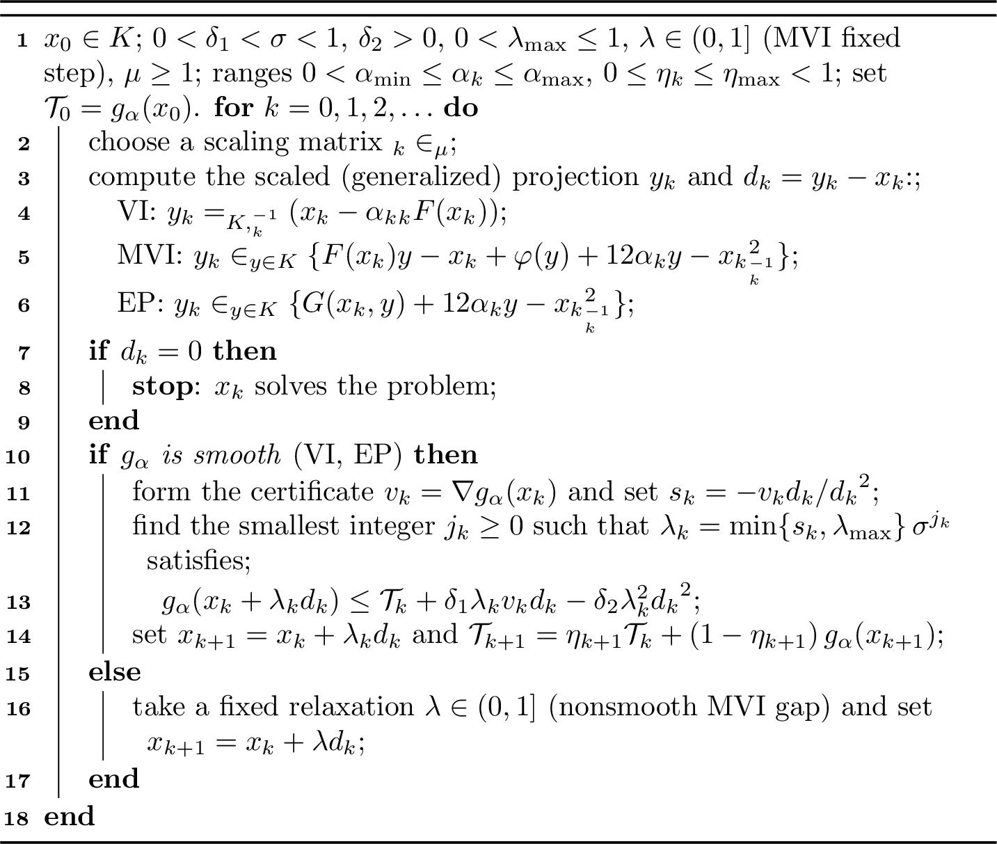
In an implementation the exact test \(d_k=0\) is replaced by \(\lVert d_k \rVert\le\varepsilon\) for a tolerance \(\varepsilon>0\), with an iteration cap as a safeguard (Section ¿sec:ss:setup-stop?).
The line-search test in Algorithm 1 reads \[\label{eq:sgm-ls-gap} g_\alpha(x_k+\lambda_k d_k)\le \mathcal{T}_k+\delta_1\lambda_k\langle v_k,\, d_k\rangle-\delta_2\lambda_k^2\lVert d_k \rVert^2 .\tag{6}\]
Assumption 10.
\(K\subseteq\mathbb{R}^n\) is nonempty, closed, and convex, and \(S\neq\emptyset\).
The relevant gap function (\(g_\alpha\) for VI/MVI, \(g_\alpha^{\mathrm{EP}}\) for EP) is coercive, so its sublevel sets are bounded. Under strong monotonicity this is automatic, since the error bound makes the gap coercive.
\(F\) is continuous (resp.\(G\) is continuous).
The scaling matrices satisfy \(\mathcal{D}_k\in\mathfrak{D}_\mu\) for all \(k\).
Assumption 11 (Direction/sufficient-decrease condition). There is \(\kappa>0\) such that the certificate \(v_k\) and direction \(d_k\) satisfy \(\langle v_k,\, d_k\rangle\le -\kappa\,\lVert d_k \rVert^2\) for all \(k\).
5 Convergence analysis↩︎
Throughout this section we analyse the smooth-gap certificate (V1) for the variational inequality 1 and fix the scaling matrix and regularization parameter: \(\mathcal{D}_k\equiv\mathcal{D}\in\mathfrak{D}_\mu\) and \(\alpha>0\) constant, so that the gap function \(g_\alpha\) of ?? is a fixed \(C^1\) function. We add the following standing hypotheses to Assumption 10.
Assumption 12 (V1 setting). \(F\in C^{1,1}\) is strongly monotone with modulus \(m>0\) and \(L\)-Lipschitz. We take \(v_k=\nabla g_\alpha(x_k)\).
The following example exhibits an operator satisfying Assumptions 10–12.
Example 1 (A genuine VI satisfying Assumptions 10–12). Let \(n=2\), \(K=[-1,1]^2\), and \(F(x)=Mx+q\) with \[M=mI+J,\qquad m=1,\qquad J=\begin{pmatrix}0&2\\-2&0\end{pmatrix},\qquad q=\begin{pmatrix}-1\\\tfrac12\end{pmatrix},\] so that \(J^\top=-J\), and take the scaling \(\mathcal{D}=I\in\mathfrak{D}_\mu\) with \(\mu=1\).
**Strong monotonicity, modulus \(m=1\): \(\langle F(x)-F(y),\, x-y\rangle=\langle M(x-y),\, x-y\rangle=m\lVert x-y \rVert^2\), since \(\langle Jd,\, d\rangle=0\) for skew-symmetric \(J\).
**Lipschitz, \(L=\lVert M \rVert_2=\sqrt5\),* because \(M^\top M=5I\).*
**A genuine VI:* \(F\) is affine with constant Jacobian \(\nabla F=M\), whose symmetric part \(\tfrac12(M+M^\top)=mI\succ0\) makes the scaled-projection step \(d=y_\alpha(x)-x\) a descent direction for \(g_\alpha\) (Proposition 3). Here \(y_\alpha(x)=P_{K,\mathcal{D}^{-1}}\!\big(x-\alpha\mathcal{D}F(x)\big)\), which for \(\mathcal{D}=I\) is the componentwise clipping of \(x-\alpha F(x)\) onto \([-1,1]^2\). The skew part \(J\neq0\) makes \(\nabla F\) asymmetric, so \(F\) is not a gradient and the problem is not an optimization.*
Since \(K\) is compact convex and \(F\) is continuous and strongly monotone, \(\mathrm{VI}(F,K)\) has a unique solution, and Assumptions 10 and 12 hold.
By Definition 4 the symmetric part of \(\nabla F\) satisfies \(\langle d,\, \nabla F(x)\,d\rangle\ge m\lVert d \rVert^2\), so the descent identity ?? gives \[\label{eq:dir-m} \langle \nabla g_\alpha(x_k),\, d_k\rangle\;\le\;-\,m\,\lVert d_k \rVert^2 ,\tag{7}\] i.e. Assumption 11 holds with \(\kappa=m\), and \(s_k=-\langle v_k,\, d_k\rangle/\lVert d_k \rVert^2\ge\kappa\). Problem 1 has a unique solution, \(x^*\), because \(F\) is strongly monotone. By Proposition 7 the error bound ?? holds globally: \[g_\alpha(x)\;\ge\;\tau\,\lVert x-x^* \rVert^2 \qquad\forall\, x\in K .\] Here \(\tau>0\) exists for every \(\alpha>0\). The explicit value \(\tau=(1-q)^2/(2\alpha\mu)\) (Proposition 18) requires the additional rate restriction \(\alpha<2m/(\mu^3L^2)\). This makes \(g_\alpha\) coercive, so the sublevel set \(\mathcal{L}_0=\{x\in K: g_\alpha(x)\le \mathcal{T}_0\}\) is bounded.
The analysis below uses the following set and estimates. Set \[\mathcal{C}_0=\operatorname{conv}\big(\mathcal{L}_0\cup y_\alpha(\mathcal{L}_0)\big)\subseteq K ,\] where \(y_\alpha\) is the scaled projection step ?? . It is a bounded convex set containing the segment \([x,y_\alpha(x)]\) for every \(x\in\mathcal{L}_0\). Because \(F\in C^{1,1}\) and \(\mathcal{C}_0\) is bounded, \(\nabla g_\alpha\) is Lipschitz on \(\mathcal{C}_0\) with a constant \(L_g\).
By Lemma 1(ii) the iterates satisfy \(x_k\in\mathcal{L}_0\), so \(\{x_k\}\) is bounded. Since \(F\) is \(L\)-Lipschitz, this gives \(M_F:=\sup_k\lVert F(x_k) \rVert<\infty\). Finally, at the maximizer \(y_\alpha(x)\) the gap equals \[g_\alpha(x)=-\langle F(x),\, d\rangle-\tfrac1{2\alpha}\lVert d \rVert_{\mathcal{D}^{-1}}^2 ,\qquad d=y_\alpha(x)-x ,\] so \[\label{eq:gap-ub} 0\;\le\;g_\alpha(x)\;\le\;-\langle F(x),\, d\rangle\;\le\;\lVert F(x) \rVert\,\lVert d \rVert .\tag{8}\]
Lemma 1 (Line search and sufficient decrease). Under Assumptions 10 and 12:
the line search terminates and \(\lambda_k\ge\lambda_{\min}:=\min\{\kappa,\lambda_{\max},\sigma\bar\lambda\}>0\), where \(\kappa\) is the direction constant of Assumption 11 (here \(\kappa=m\) by 7 ) and \[\bar\lambda=(1-\delta_1)\kappa/(L_g/2+\delta_2).\]
\(g_\alpha(x_k)\le\mathcal{T}_k\) for all \(k\), and \(\{\mathcal{T}_k\}\) is nonincreasing.
\(\mathcal{T}_k-\mathcal{T}_{k+1}\ge (1-\eta_{\max})\,\rho\,\lVert d_k \rVert^2\) with \(\rho=\delta_1\kappa\lambda_{\min}>0\).
We argue by induction that \(g_\alpha(x_k)\le\mathcal{T}_k\) for all \(k\). This holds at \(k=0\) because \(\mathcal{T}_0=g_\alpha(x_0)\). Assume it at index \(k\), so \(x_k\in\mathcal{L}_0\).
For \(0<\lambda\le\lambda_{\max}\le1\) the trial point \(x_k+\lambda d_k\) lies on \([x_k,y_\alpha(x_k)]\subseteq\mathcal{C}_0\), so the descent lemma for the \(L_g\)-Lipschitz gradient on \(\mathcal{C}_0\) gives \[g_\alpha(x_k+\lambda d_k)\;\le\;g_\alpha(x_k)+\lambda\langle \nabla g_\alpha(x_k),\, d_k\rangle +\tfrac{L_g}{2}\lambda^2\lVert d_k \rVert^2 .\] With \(g_\alpha(x_k)\le\mathcal{T}_k\) and \(v_k=\nabla g_\alpha(x_k)\), the test 6 holds whenever \[\big(\tfrac{L_g}{2}+\delta_2\big)\lambda\lVert d_k \rVert^2\;\le\;(1-\delta_1)\big(-\langle \nabla g_\alpha(x_k),\, d_k\rangle\big) ,\] which by 7 is true for all \(0<\lambda\le\bar\lambda\). Hence the backtracking terminates. Its first trial is \(\min\{s_k,\lambda_{\max}\}\ge\min\{\kappa,\lambda_{\max}\}\) and the trials shrink by \(\sigma\in(0,1)\). A trial fails only when it exceeds \(\bar\lambda\), so the accepted step satisfies \(\lambda_k\ge\min\{\kappa,\lambda_{\max},\sigma\bar\lambda\}=\lambda_{\min}\).
The accepted step obeys 6 , hence \[g_\alpha(x_{k+1})\;\le\;\mathcal{T}_k+\delta_1\lambda_k\langle \nabla g_\alpha(x_k),\, d_k\rangle -\delta_2\lambda_k^2\lVert d_k \rVert^2\;\le\;\mathcal{T}_k .\] Therefore \(\mathcal{T}_{k+1}=\eta_{k+1}\mathcal{T}_k+(1-\eta_{k+1})g_\alpha(x_{k+1})\le\mathcal{T}_k\), and \[\mathcal{T}_{k+1}-g_\alpha(x_{k+1})=\eta_{k+1}\big(\mathcal{T}_k-g_\alpha(x_{k+1})\big)\ge0.\] This closes the induction and shows \(\{\mathcal{T}_k\}\) is nonincreasing.
Using 7 , \(\lambda_k\ge\lambda_{\min}\), and \(\eta_{k+1}\le\eta_{\max}\), \[\begin{array}{lcl} \mathcal{T}_k-\mathcal{T}_{k+1}&=&(1-\eta_{k+1})\big(\mathcal{T}_k-g_\alpha(x_{k+1})\big) \\ \;&\ge& \;(1-\eta_{\max})\big(-\delta_1\lambda_k\langle \nabla g_\alpha(x_k),\, d_k\rangle\big) \\ \;&\ge&\;(1-\eta_{\max})\,\delta_1\kappa\lambda_{\min}\lVert d_k \rVert^2=(1-\eta_{\max})\,\rho\,\lVert d_k \rVert^2 . \end{array}\]
Remark 13 (Reusability of Lemma 1). The proof of Lemma 1 uses only that \(g_\alpha\) is nonnegative and \(C^1\) with \(L_g\)-Lipschitz gradient on \(\mathcal{C}_0\), and the direction bound \(\langle v_k,\, d_k\rangle\le-\kappa\lVert d_k \rVert^2\) of Assumption 11. The lemma therefore holds with \(g_\alpha\) replaced by any function with these properties. Theorem 23 applies it to the equilibrium gap \(g_\alpha^{\mathrm{EP}}\).
Theorem 14 (Global convergence, V1). Under Assumptions 10 and 12, the series \(\sum_{k}\lVert d_k \rVert^2\) is convergent and the iterates \(x_k\) converge to the unique solution \(x^*\) of 1 , with \(g_\alpha(x_k)\to0\).
By Lemma 1(iii), summed over \(k=0,\dots,N\) and telescoped, \[(1-\eta_{\max})\,\rho\sum_{k=0}^{N}\lVert d_k \rVert^2\;\le\;\mathcal{T}_0-\mathcal{T}_{N+1}\;\le\;\mathcal{T}_0 ,\] because \(\mathcal{T}_{N+1}\ge g_\alpha(x_{N+1})\ge0\). Letting \(N\to\infty\) gives \(\sum_{k}\lVert d_k \rVert^2<\infty\), hence \(\lVert d_k \rVert\to0\). By 8 , \[g_\alpha(x_k)\le\lVert F(x_k) \rVert\lVert d_k \rVert\le M_F\lVert d_k \rVert\to0.\] Finally, the error bound \(g_\alpha(x_k)\ge\tau\lVert x_k-x^* \rVert^2\) gives \(\lVert x_k-x^* \rVert^2\le g_\alpha(x_k)/\tau\to0\), so \(x_k\to x^*\).
Corollary 1 (Best-iterate sublinear rate). Under Assumptions 10 and 12, for every \(N\), \[\min_{0\le k\le N}\lVert d_k \rVert^2\;\le\;\frac{\mathcal{T}_0}{(1-\eta_{\max})\,\rho\,(N+1)} ,\] so \(\displaystyle \min_{0\le k\le N}\lVert d_k \rVert=O(1/\sqrt{N})\) and, by 8 , \(\displaystyle\min_{0\le k\le N}g_\alpha(x_k)=O(1/\sqrt{N})\). The bound is informative only when the direction constant is positive (here \(\kappa=m>0\), so \(\rho=\delta_1\kappa\lambda_{\min}>0\)). By Remark 13 it holds for any merit satisfying the direction condition, so a merely monotone operator, for which the direction condition holds only with \(\kappa=0\), is not covered.
The proof of Theorem 14 gives \(\displaystyle (1-\eta_{\max})\,\rho\sum_{k=0}^{N}\lVert d_k \rVert^2\le\mathcal{T}_0,\) and \(\displaystyle\min_{0\le k\le N}\lVert d_k \rVert^2\le\tfrac{1}{N+1}\sum_{k=0}^{N}\lVert d_k \rVert^2\) yields the bound \[\min_{0\le k\le N}\lVert d_k \rVert^2\;\le\;\frac{\mathcal{T}_0}{(1-\eta_{\max})\,\rho\,(N+1)}.\] The gap estimate follows from \(g_\alpha(x_k)\le M_F\lVert d_k \rVert\) in 8 .
Theorem 15 (R-linear convergence, V1). Under Assumptions 10 and 12, suppose moreover that \(\alpha\in\big(0,\,2m/(\mu^3L^2)\big)\), and set \[q=\sqrt{1-\tfrac{2\alpha m}{\mu}+\alpha^2\mu^2L^2}\in[0,1),\qquad \theta=1-\lambda_{\min}(1-q)\in(0,1).\] Then the iterates \(x_k\) converge to \(x^*\) R-linearly with ratio \(\theta\), that is, \[\label{eq:rate} \lVert x_k-x^* \rVert\;\le\;\mu\,\theta^{k}\,\lVert x_0-x^* \rVert\qquad\text{for all }k,\qquad{(8)}\] and the gap converges R-linearly with the same ratio, \(g_\alpha(x_k)\le C_g\,\theta^{k}\) for some \(C_g>0\).
Set \(e_k=x_k-x^*\) and write \(\lVert \cdot \rVert_*=\lVert \cdot \rVert_{\mathcal{D}^{-1}}\). The step map \(T(x)=P_{K,\mathcal{D}^{-1}}(x-\alpha\mathcal{D}F(x))=y_\alpha(x)\) has \(x^*\) as a fixed point by Proposition 9, and \(y_k=T(x_k)\). By Remark 1, \(\lVert x \rVert_{\mathcal{D}}\) and \(\lVert x \rVert_*\) lie in \([\tfrac{1}{\sqrt\mu}\lVert x \rVert,\,\sqrt\mu\,\lVert x \rVert]\) for every \(x\).
We first show that \(T\) contracts in \(\lVert \cdot \rVert_*\). As \(P_{K,\mathcal{D}^{-1}}\) is nonexpansive in \(\lVert \cdot \rVert_*\), \[\label{eq:rate-exp} \lVert y_k-x^* \rVert_*^2\le\lVert e_k-\alpha\mathcal{D}\big(F(x_k)-F(x^*)\big) \rVert_*^2 =\lVert e_k \rVert_*^2-2\alpha\langle e_k,\, F(x_k)-F(x^*)\rangle+\alpha^2\lVert F(x_k)-F(x^*) \rVert_{\mathcal{D}}^2 .\tag{9}\] Strong monotonicity and \(L\)-Lipschitz continuity, together with the norm bounds above, give \[\label{eq:rate-bd} \langle e_k,\, F(x_k)-F(x^*)\rangle\ge\tfrac{m}{\mu}\lVert e_k \rVert_*^2 ,\qquad \lVert F(x_k)-F(x^*) \rVert_{\mathcal{D}}^2\le\mu^2L^2\lVert e_k \rVert_*^2 .\tag{10}\] Substituting 10 into 9 yields \[\label{eq:rate-q} \lVert y_k-x^* \rVert_*\;\le\;q\,\lVert e_k \rVert_* ,\qquad q^2=1-\tfrac{2\alpha m}{\mu}+\alpha^2\mu^2L^2 ,\tag{11}\] and \(q<1\) because \(\alpha<2m/(\mu^3L^2)\). Since \(x_{k+1}=(1-\lambda_k)x_k+\lambda_k y_k\) with \(\lambda_k\in[\lambda_{\min},1]\), the relaxed step inherits the contraction 11 : \[\label{eq:rate-relax} \lVert e_{k+1} \rVert_*\le(1-\lambda_k)\lVert e_k \rVert_*+\lambda_k\lVert y_k-x^* \rVert_* \le\big(1-\lambda_k(1-q)\big)\lVert e_k \rVert_*\le\theta\,\lVert e_k \rVert_* .\tag{12}\] Iterating 12 gives \(\lVert e_k \rVert_*\le\theta^k\lVert e_0 \rVert_*\). Converting back to the Euclidean norm, \[\lVert x_k-x^* \rVert\le\sqrt\mu\,\lVert e_k \rVert_*\le\sqrt\mu\,\theta^k\lVert e_0 \rVert_*\le\mu\,\theta^k\lVert x_0-x^* \rVert ,\] which is ?? . Finally, \(\lVert d_k \rVert\le\big(1+\mu(1+\alpha\mu L)\big)\lVert e_k \rVert\) by Lipschitz continuity of \(y_\alpha\) together with \(y_\alpha(x^*)=x^*\), so 8 gives \(g_\alpha(x_k)\le M_F\lVert d_k \rVert\le C_g\,\theta^k\).
Remark 16. The R-linear rate does not come from the sufficient decrease of Lemma 1 alone. Its per-step estimate \(\mathcal{T}_k-\mathcal{T}_{k+1}\ge(1-\eta_{\max})\rho\,\lVert d_k \rVert^2\) is quadratic in the residual, so it controls only \(\sum_k\lVert d_k \rVert^2\) and gives the sublinear rate of Corollary 1. An R-linear rate from this estimate alone would need the per-step decrease to be proportional to \(g_\alpha(x_k)\), that is, a bound \(g_\alpha(x)\le C\lVert d \rVert^2\). No such bound holds: by ?? and 8 , \[\tfrac{1}{2\alpha}\lVert d \rVert_{\mathcal{D}^{-1}}^2\;\le\;g_\alpha(x)\;\le\;\lVert F(x) \rVert\,\lVert d \rVert ,\] and the linear upper bound is sharp at a solution \(x^*\) on the boundary of \(K\), where \(d=0\) but \(\nabla g_\alpha(x^*)=F(x^*)\ne0\) (Remark 4).
The R-linear rate of Theorem 15 comes instead from the contraction 11 , which strong monotonicity provides. With the error bound ?? and the bounds ?? and 8 , it makes the distance \(\lVert x_k-x^* \rVert\), the residual \(\lVert d_k \rVert\), and the gap \(g_\alpha(x_k)\) converge to \(0\) R-linearly with the same ratio \(\theta\) (Corollary 2). For the same reason, convergence is measured by \(g_\alpha(x_k)\) or \(\lVert d_k \rVert\) rather than by \(\lVert \nabla g_\alpha(x_k) \rVert\), which need not tend to \(0\).
Remark 17 (Rate on Example 1). The rate window of Theorem 15 is nonempty. With \(\mathcal{D}=I\) (\(\mu=1\)), \(m=1\), and \(L=\sqrt5\), it is \(2m/(\mu^3L^2)=0.4\), and \(\alpha=0.2\) gives \[q=\sqrt{1-\tfrac{2\alpha m}{\mu}+\alpha^2\mu^2L^2}=\sqrt{0.8}\approx0.894\in[0,1) ,\] so the iterates converge R-linearly.
The next example shows that \(F\) need not be affine.
Example 2 (A nonlinear VI satisfying Assumptions 10–12). Let \(n=2\), \(K=[0,1]^2\), and \(F(x)=\nabla\psi(x)+Jx+q\) with \[\psi(x)=\tfrac12\lVert x \rVert^2+\tfrac16\big(x_1^3+x_2^3\big),\qquad J=\begin{pmatrix}0&2\\-2&0\end{pmatrix},\qquad q=\begin{pmatrix}-\tfrac32\\\tfrac12\end{pmatrix},\] so that \(F(x)=\big(x_1+\tfrac12x_1^2+2x_2-\tfrac32,\;-2x_1+x_2+\tfrac12x_2^2+\tfrac12\big)^\top\) is quadratic, and take the scaling \(\mathcal{D}=I\in\mathfrak{D}_\mu\) with \(\mu=1\). Its Jacobian is \[\nabla F(x)=\begin{pmatrix}1+x_1&2\\-2&1+x_2\end{pmatrix}.\]
**Strong monotonicity, modulus \(m=1\):* the symmetric part of \(\nabla F(x)\) is \(\operatorname{diag}(1+x_1,1+x_2)\succeq I\) on \(K\), so integrating \(\nabla F\) along the segment \([y,x]\subseteq K\) gives \(\langle F(x)-F(y),\, x-y\rangle\ge\lVert x-y \rVert^2\), the skew part contributing nothing to the quadratic form.*
**Lipschitz, \(L=3\):* \(L=\max_{x\in K}\lVert \nabla F(x) \rVert_2=3\), attained at \(x=(1,0)\), where \(\nabla F^\top\nabla F\) has largest eigenvalue \(9\).*
**A genuine nonlinear VI:* \(F\) is quadratic, and \(\nabla F\) carries the nonzero constant skew part \(J\), so \(F\) is not a gradient. The problem is neither affine nor an optimization.*
Since \(K\) is compact convex and \(F\) is continuous, strongly monotone, and \(C^{1,1}\) on \(K\), \(\mathrm{VI}(F,K)\) has a unique solution, and Assumptions 10 and 12 hold. The rate window of Theorem 15 is nonempty, \(2m/(\mu^3L^2)=\tfrac29\), and \(\alpha=\tfrac19\) gives \(q=\sqrt{1-\tfrac{2\alpha m}{\mu}+\alpha^2\mu^2L^2}=\sqrt{\tfrac89}=\tfrac{2\sqrt2}{3}\approx0.943\in[0,1)\), so the iterates converge R-linearly.
5.1 Error bound and merit equivalence↩︎
Theorem 15 measures convergence through the regularized gap \(g_\alpha\). We now relate this gap to the other quantities that measure progress toward the solution, chiefly the distance and the residual. The next proposition answers this, and the same relations are reused for equilibrium problems (Section 5.4).
Proposition 18 (Error bound and merit equivalence, V1). Under Assumptions 10 and 12, suppose moreover that \(\alpha\in\big(0,2m/(\mu^3L^2)\big)\), and set \(q=\sqrt{1-\tfrac{2\alpha m}{\mu}+\alpha^2\mu^2L^2}\in[0,1)\). Write \(\lVert \cdot \rVert_*=\lVert \cdot \rVert_{\mathcal{D}^{-1}}\). For \(x\in K\) and \(t>0\), the scaled residual at step size \(t\) is \[d_t(x)=y_t(x)-x ,\qquad y_t(x)=P_{K,\mathcal{D}^{-1}}\!\big(x-t\mathcal{D}F(x)\big).\] In particular, \(d_\alpha(x)=y_\alpha(x)-x\) is the residual \(d\) of ?? , with \(d_k=d_\alpha(x_k)\). Then the following hold for all \(x\in K\).
The scaled residual satisfies, \[\label{eq:res-eb} (1-q)\,\lVert x-x^* \rVert_*\;\le\;\lVert d_\alpha(x) \rVert_* ,\qquad \lVert d_t(x) \rVert\;\le\;\big(1+\mu(1+t\mu L)\big)\,\lVert x-x^* \rVert\quad(t>0).\qquad{(9)}\]
The regularized gap is an explicit error bound for the distance to \(S=\{x^*\}\), \[\label{eq:eb-explicit} g_\alpha(x)\;\ge\;\tau\,\mathop{\mathrm{dist}}(x,S)^2 ,\qquad \tau=\frac{(1-q)^2}{2\alpha\mu} .\qquad{(10)}\]
For \(0<\alpha<\beta\) the D-gap satisfies, \[\label{eq:dgap-twosided} \tfrac12\big(\tfrac1\alpha-\tfrac1\beta\big)\lVert d_\alpha(x) \rVert_*^2 \;\le\;g_{\alpha\beta}(x)\;\le\; \tfrac12\big(\tfrac1\alpha-\tfrac1\beta\big)\lVert d_\beta(x) \rVert_*^2 .\qquad{(11)}\]
If moreover \(\beta<2m/(\mu^3L^2)\), then \(\mathop{\mathrm{dist}}(x,S)^2\), \(\lVert d_\alpha(x) \rVert^2\), \(\lVert d_\beta(x) \rVert^2\), and \(g_{\alpha\beta}(x)\) are mutually equivalent on \(K\), i.e.there are constants \(0<\underline{c}\le\overline{c}\) such that \[\underline{c}\,\mathop{\mathrm{dist}}(x,S)^2\;\le\;\lVert d_\alpha(x) \rVert^2,\;\;\lVert d_\beta(x) \rVert^2,\;\;g_{\alpha\beta}(x) \;\le\;\overline{c}\,\mathop{\mathrm{dist}}(x,S)^2 \qquad(x\in K).\]
The proof of Theorem 15 shows that \[\lVert y_\alpha(x)-x^* \rVert_*\le q\lVert x-x^* \rVert_*, \quad \text{where}\quad y_\alpha(x^*)=x^*.\] Therefore \[\lVert x-x^* \rVert_*\;\le\;\lVert d_\alpha(x) \rVert_*+\lVert y_\alpha(x)-x^* \rVert_* \;\le\;\lVert d_\alpha(x) \rVert_*+q\,\lVert x-x^* \rVert_* ,\] which rearranges to the first inequality of ?? . For the second, fix \(t>0\). Since \(x^*\) solves 1 , it is a fixed point of the scaled projection step at every step size, so \(y_t(x^*)=x^*\) (Proposition 9). The projection \(P_{K,\mathcal{D}^{-1}}\) is Lipschitz with constant \(\mu\) in the Euclidean norm (Remark 2, since \(\mathcal{D}^{-1}\in\mathfrak{D}_\mu\)). Writing \(u=x-t\mathcal{D}F(x)\) and \(u^*=x^*-t\mathcal{D}F(x^*)\), so that \(y_t(x)=P_{K,\mathcal{D}^{-1}}(u)\) and \(y_t(x^*)=P_{K,\mathcal{D}^{-1}}(u^*)=x^*\), \[\lVert y_t(x)-x^* \rVert\;\le\;\mu\,\lVert u-u^* \rVert \;=\;\mu\,\lVert (x-x^*)-t\mathcal{D}\big(F(x)-F(x^*)\big) \rVert .\] By the triangle inequality, \(\lVert \mathcal{D} \rVert\le\mu\) (Remark 1), and the \(L\)-Lipschitz continuity of \(F\), \[\lVert u-u^* \rVert\;\le\;\lVert x-x^* \rVert+t\,\lVert \mathcal{D} \rVert\,\lVert F(x)-F(x^*) \rVert\;\le\;(1+t\mu L)\,\lVert x-x^* \rVert ,\] so that \(\lVert y_t(x)-x^* \rVert\le\mu(1+t\mu L)\lVert x-x^* \rVert\). Finally \(d_t(x)=\big(y_t(x)-x^*\big)-\big(x-x^*\big)\), and the triangle inequality gives \[\lVert d_t(x) \rVert\;\le\;\lVert y_t(x)-x^* \rVert+\lVert x-x^* \rVert\;\le\;\big(1+\mu(1+t\mu L)\big)\lVert x-x^* \rVert ,\] which is the second inequality of ?? .
By the lower bound ?? , the first inequality of ?? , and \(\lVert \cdot \rVert_*^2\ge\tfrac1\mu\lVert \cdot \rVert^2\), \[g_\alpha(x)\;\ge\;\tfrac1{2\alpha}\lVert d_\alpha(x) \rVert_*^2 \;\ge\;\tfrac{(1-q)^2}{2\alpha}\lVert x-x^* \rVert_*^2 \;\ge\;\tfrac{(1-q)^2}{2\alpha\mu}\lVert x-x^* \rVert^2 ,\] which is ?? .
Write \(\Phi_t(y)=\langle F(x),\, x-y\rangle-\tfrac1{2t}\lVert y-x \rVert_{\mathcal{D}^{-1}}^2\) for the \(t\)-objective of ?? , so that \(g_t(x)=\max_{y\in K}\Phi_t(y)=\Phi_t(y_t(x))\). Since \(y_t(x)\) is the maximizer and \(\lVert y_t(x)-x \rVert_{\mathcal{D}^{-1}}=\lVert d_t(x) \rVert_*\), \[g_\alpha(x)=\langle F(x),\, x-y_\alpha(x)\rangle-\tfrac1{2\alpha}\lVert d_\alpha(x) \rVert_*^2 ,\qquad g_\beta(x)=\langle F(x),\, x-y_\beta(x)\rangle-\tfrac1{2\beta}\lVert d_\beta(x) \rVert_*^2 .\] For the lower bound, \(y_\alpha(x)\in K\) is feasible for the \(\beta\)-maximization, so \[g_\beta(x)\;\ge\;\Phi_\beta(y_\alpha(x))\;=\;\langle F(x),\, x-y_\alpha(x)\rangle-\tfrac1{2\beta}\lVert d_\alpha(x) \rVert_*^2 .\] Subtracting the identity for \(g_\alpha(x)\), the inner-product terms cancel and \[g_{\alpha\beta}(x)=g_\beta(x)-g_\alpha(x)\;\ge\;\Big(\tfrac1{2\alpha}-\tfrac1{2\beta}\Big)\lVert d_\alpha(x) \rVert_*^2 =\tfrac12\Big(\tfrac1\alpha-\tfrac1\beta\Big)\lVert d_\alpha(x) \rVert_*^2 ,\] the lower bound of ?? . Symmetrically, \(y_\beta(x)\in K\) is feasible for the \(\alpha\)-maximization, so \(g_\alpha(x)\ge\Phi_\alpha(y_\beta(x))=\langle F(x),\, x-y_\beta(x)\rangle-\tfrac1{2\alpha}\lVert d_\beta(x) \rVert_*^2\). Subtracting this from the identity for \(g_\beta(x)\) gives \[g_{\alpha\beta}(x)\;\le\;\Big(\tfrac1{2\alpha}-\tfrac1{2\beta}\Big)\lVert d_\beta(x) \rVert_*^2 =\tfrac12\Big(\tfrac1\alpha-\tfrac1\beta\Big)\lVert d_\beta(x) \rVert_*^2 ,\] the upper bound.
Recall \(\mathop{\mathrm{dist}}(x,S)=\lVert x-x^* \rVert\). By the contraction estimate in the proof of Theorem 15, applied at step size \(t\), \[\lVert y_t(x)-x^* \rVert_*\;\le\;q_t\,\lVert x-x^* \rVert_* ,\qquad q_t=\sqrt{1-\tfrac{2tm}{\mu}+t^2\mu^2L^2} ,\] and \(q_t<1\) precisely when \(t<2m/(\mu^3L^2)\), which holds for both \(t=\alpha\) and \(t=\beta\). As in (i), the triangle inequality gives the residual lower bound \((1-q_t)\lVert x-x^* \rVert_*\le\lVert d_t(x) \rVert_*\). Combining it with the upper bound of (i) and the norm equivalence (Remark 1) gives, for \(t\in\{\alpha,\beta\}\), \[\label{eq:res-bounds} \frac{(1-q_t)^2}{\mu^2}\,\mathop{\mathrm{dist}}(x,S)^2\;\le\;\lVert d_t(x) \rVert^2 \;\le\;\big(1+\mu(1+t\mu L)\big)^2\,\mathop{\mathrm{dist}}(x,S)^2 ,\tag{13}\] so \(\lVert d_\alpha(x) \rVert^2\) and \(\lVert d_\beta(x) \rVert^2\) are each equivalent to \(\mathop{\mathrm{dist}}(x,S)^2\). Combining ?? with the residual bounds yields \[\label{eq:dgap-bounds} \frac{(1-q_\alpha)^2}{2\mu}\Big(\tfrac1\alpha-\tfrac1\beta\Big)\mathop{\mathrm{dist}}(x,S)^2 \;\le\;g_{\alpha\beta}(x)\;\le\; \frac{\mu}{2}\Big(\tfrac1\alpha-\tfrac1\beta\Big)\big(1+\mu(1+\beta\mu L)\big)^2\mathop{\mathrm{dist}}(x,S)^2 ,\tag{14}\] so \(g_{\alpha\beta}(x)\) is equivalent to \(\mathop{\mathrm{dist}}(x,S)^2\) too. Taking \(\underline{c}\) to be the least and \(\overline{c}\) the greatest of the positive constants in 13 and 14 gives \[\underline{c}\,\mathop{\mathrm{dist}}(x,S)^2\le\lVert d_\alpha(x) \rVert^2,\lVert d_\beta(x) \rVert^2,g_{\alpha\beta}(x)\le\overline{c}\,\mathop{\mathrm{dist}}(x,S)^2.\]
Corollary 2 (R-linear in every natural measure). Under the hypotheses of Theorem 15, the distance \(\mathop{\mathrm{dist}}(x_k,S)\), the residual \(\lVert d_\alpha(x_k) \rVert\), and the regularized gap \(g_\alpha(x_k)\) converge to \(0\) R-linearly with ratio \(\theta\), while the squared residual and the D-gap \(g_{\alpha\beta}(x_k)\) (for \(\alpha<\beta<2m/(\mu^3L^2)\)) converge with ratio \(\theta^2\).
Theorem 15 gives \(\mathop{\mathrm{dist}}(x_k,S)=\lVert x_k-x^* \rVert\le\mu\theta^k\lVert x_0-x^* \rVert=O(\theta^k)\), so the distance converges R-linearly with ratio \(\theta\). The residual and the gap inherit this rate: the upper bound in ?? gives \(\lVert d_\alpha(x_k) \rVert\le\big(1+\mu(1+\alpha\mu L)\big)\lVert x_k-x^* \rVert= O(\theta^k)\), and 8 gives \(g_\alpha(x_k)\le M_F\lVert d_\alpha(x_k) \rVert=O(\theta^k)\).
Squaring, \(\lVert d_\alpha(x_k) \rVert^2=O(\theta^{2k})\). For the D-gap, the upper bound in ?? , the norm equivalence \(\lVert \cdot \rVert_*^2\le\mu\lVert \cdot \rVert^2\), and the residual bound at \(t=\beta\) give \(g_{\alpha\beta}(x_k)\le\tfrac{\mu}{2}\big(\tfrac1\alpha-\tfrac1\beta\big)\lVert d_\beta(x_k) \rVert^2=O(\theta^{2k})\). Hence the squared residual and the D-gap converge with ratio \(\theta^2\).
5.2 Variable metric↩︎
Theorems 14–15 fix the scaling matrix. We now let it vary with \(k\), taking \(\mathcal{D}_k\in\mathfrak{D}_\mu\), and write \(g_{\alpha,\mathcal{D}_k}\) for the gap ?? with \(\mathcal{D}=\mathcal{D}_k\). The contraction behind Theorem 15 uses only the spectral bounds of \(\mathfrak{D}_\mu\), so it holds with the same \(q\) in each \(\mathcal{D}_k^{-1}\)-norm. The moving-average reference of the line search compares values of the changing merit \(g_{\alpha,\mathcal{D}_k}\), so here we drive the iteration with a fixed relaxation step \(\lambda\in(0,1]\) instead. The next theorem shows that a summable change in the scaling matrices then preserves the R-linear rate, inflating only its constant.
Theorem 19 (Variable metric, V1). Under Assumptions 10 and 12, suppose moreover that \(\alpha\in(0,2m/(\mu^3L^2))\) and \(\sum_{k\ge0}\lVert \mathcal{D}_{k+1}^{-1}-\mathcal{D}_k^{-1} \rVert<\infty\) in the spectral norm. Run the relaxed iteration \(x_{k+1}=(1-\lambda)x_k+\lambda\,y_{\alpha,\mathcal{D}_k}(x_k)\) with a fixed step \(\lambda\in(0,1]\), and set \[q=\sqrt{1-\tfrac{2\alpha m}{\mu}+\alpha^2\mu^2L^2}\in[0,1),\qquad \theta=1-\lambda(1-q)\in(0,1),\] and \(M=\exp\!\big(\mu\sum_{k\ge0}\lVert \mathcal{D}_{k+1}^{-1}-\mathcal{D}_k^{-1} \rVert\big)\). Then \(x_k\) converges to \(x^*\) R-linearly with ratio \(\theta\), that is, \[\lVert x_k-x^* \rVert\;\le\;\mu\sqrt M\,\theta^{k}\,\lVert x_0-x^* \rVert\qquad\text{for all }k.\] When \(\mathcal{D}_k\equiv\mathcal{D}\), \(M=1\) and the bound reduces to Theorem 15.
Let \(V_k=\lVert x_k-x^* \rVert_{\mathcal{D}_k^{-1}}^2\). We bound \(V_{k+1}\) in two steps: the step map contracts in the current \(\mathcal{D}_k^{-1}\)-norm, and changing the scaling matrix perturbs \(V\) by a summable factor.
In the \(\mathcal{D}_k^{-1}\)-norm, the contraction in the proof of Theorem 15 applies with \(\mathcal{D}=\mathcal{D}_k\). Its constant \(q\) uses only the spectral bounds \([1/\mu,\mu]\), not the particular \(\mathcal{D}_k\), so \[\lVert y_k-x^* \rVert_{\mathcal{D}_k^{-1}}\;\le\;q\,\lVert x_k-x^* \rVert_{\mathcal{D}_k^{-1}}\] holds for every \(k\). With the fixed step \(x_{k+1}=(1-\lambda)x_k+\lambda y_k\), \(\lambda\in(0,1]\), convexity of \(\lVert \cdot \rVert_{\mathcal{D}_k^{-1}}\) gives \[\label{eq:vm-contract} \lVert x_{k+1}-x^* \rVert_{\mathcal{D}_k^{-1}}\;\le\;\big(1-\lambda(1-q)\big)\lVert x_k-x^* \rVert_{\mathcal{D}_k^{-1}} \;=\;\theta\,\lVert x_k-x^* \rVert_{\mathcal{D}_k^{-1}} .\tag{15}\] Writing \(\epsilon_k=\lVert \mathcal{D}_{k+1}^{-1}-\mathcal{D}_k^{-1} \rVert\) and using \(\lVert v \rVert^2\le\mu\lVert v \rVert_{\mathcal{D}_k^{-1}}^2\) (Remark 1) together with 15 , \[V_{k+1}=\lVert x_{k+1}-x^* \rVert_{\mathcal{D}_{k+1}^{-1}}^2 \;\le\;\lVert x_{k+1}-x^* \rVert_{\mathcal{D}_k^{-1}}^2+\epsilon_k\lVert x_{k+1}-x^* \rVert^2 \;\le\;(1+\mu\epsilon_k)\,\theta^2 V_k .\] Iterating this recursion from \(V_0\) gives \[V_k\;\le\;\Big(\prod_{j=0}^{k-1}(1+\mu\epsilon_j)\Big)\theta^{2k}V_0 .\] Since \(\sum_j\epsilon_j<\infty\) and \(1+t\le e^t\), the product is bounded uniformly in \(k\), \[\prod_{j=0}^{k-1}(1+\mu\epsilon_j)\;\le\;\prod_{j\ge0}(1+\mu\epsilon_j) \;\le\;\exp\!\Big(\mu\sum_{j\ge0}\epsilon_j\Big)\;=\;M ,\] so \(V_k\le M\theta^{2k}V_0\). Converting back to the Euclidean norm by Remark 1, we have \[\begin{array}{lcl} \lVert x_k-x^* \rVert^2\;\le\;\mu V_k\;&\le&\;\mu M\theta^{2k}V_0\\[2mm] &=& \mu M\theta^{2k}\lVert x_0-x^* \rVert_{\mathcal{D}_0^{-1}}^2 \\[2mm] &\le& \mu^2 M\theta^{2k}\lVert x_0-x^* \rVert^2 \\[2mm] \end{array}\] and taking square roots gives \(\lVert x_k-x^* \rVert\le\mu\sqrt M\,\theta^k\lVert x_0-x^* \rVert\).
Remark 20. The hypothesis \(\sum_k\lVert \mathcal{D}_{k+1}^{-1}-\mathcal{D}_k^{-1} \rVert<\infty\) makes the consecutive changes summable, so the inverse scaling matrices converge, \(\mathcal{D}_k^{-1}\to\bar\mathcal{D}^{-1}\) for some \(\bar\mathcal{D}\in\mathfrak{D}_\mu\). It implies the variable-metric condition \[(1+\eta_k)\mathcal{D}_k^{-1}\succeq\mathcal{D}_{k+1}^{-1}, \quad \sum_k\eta_k<\infty,\] of Combettes–Vũ [16], where \(A\succeq B\) means \(A-B\) is positive semidefinite and \[\eta_k=\mu\lVert \mathcal{D}_{k+1}^{-1}-\mathcal{D}_k^{-1} \rVert.\] Under it the variation of the scaling matrix costs nothing in the rate: the bound of Theorem 19 keeps the fixed-metric ratio \(\theta\) and inflates only the constant, by \(\sqrt M=\exp\!\big(\tfrac\mu2\sum_k\lVert \mathcal{D}_{k+1}^{-1}-\mathcal{D}_k^{-1} \rVert\big)\).
5.3 Mixed variational inequalities↩︎
The smooth-gap route (V1) used \(g_\alpha\in C^1\), which fails when the nonsmooth term \(\varphi\) is present. The strong-monotone rate, however, rests on the contraction of the step map, and this carries over once the projection is replaced by the scaled resolvent. For 2 the inner subproblem is solved by the scaled forward–backward step \[y_\alpha(x)=\mathop{\mathrm{prox}}^{\mathcal{D}^{-1}}_{\alpha(\varphi+\iota_K)}\!\big(x-\alpha\mathcal{D}F(x)\big) \in\mathop{\mathrm{arg\,min}}_{y\in K}\Big\{\langle F(x),\, y-x\rangle+\varphi(y)+\tfrac1{2\alpha}\lVert y-x \rVert_{\mathcal{D}^{-1}}^2\Big\},\] with \(\iota_K\) the indicator of \(K\) and \(\mathop{\mathrm{prox}}^{\mathcal{D}^{-1}}\) the scaled proximal operator (Definition 3). The MVI gap is \[g_\alpha^{\mathrm{MVI}}(x)=-\min_{y\in K}\Big\{\langle F(x),\, y-x\rangle+\varphi(y)-\varphi(x)+\tfrac1{2\alpha}\lVert y-x \rVert_{\mathcal{D}^{-1}}^2\Big\}\;\ge\;0,\] vanishing iff \(x\) solves 2 (Proposition 9(ii) with \(G(x,y)=\langle F(x),\, y-x\rangle+\varphi(y)-\varphi(x)\), convex in \(y\)). The optimality of \(y_\alpha(x)\) for the subproblem gives (cf.the VI bound ?? ) \(g_\alpha^{\mathrm{MVI}}(x)\ge\tfrac1{2\alpha}\lVert d \rVert_{\mathcal{D}^{-1}}^2\) with \(d=y_\alpha(x)-x\).
Theorem 21 (Mixed VI, strongly monotone). Under Assumption 10, suppose moreover that \(F\) is strongly monotone with modulus \(m\) and \(L\)-Lipschitz, \(\varphi\) is proper, convex, and lower semicontinuous, and \(\alpha\in(0,2m/(\mu^3L^2))\). Let the scaling matrices be fixed (\(\mathcal{D}_k\equiv\mathcal{D}\)) or vary with \(\sum_k\lVert \mathcal{D}_{k+1}^{-1}-\mathcal{D}_k^{-1} \rVert<\infty\), take a fixed relaxation step \(\lambda\in(0,1]\), and set \[q=\sqrt{1-\tfrac{2\alpha m}{\mu}+\alpha^2\mu^2L^2}\in[0,1),\qquad \theta=1-\lambda(1-q)\in(0,1).\] Then 2 has a unique solution \(x^*\), and the relaxed iteration \(x_{k+1}=(1-\lambda)x_k+\lambda\,y_{\alpha,\mathcal{D}_k}(x_k)\) has the following properties.
The iterates converge to \(x^*\) R-linearly with ratio \(\theta\), \[\lVert x_k-x^* \rVert\;\le\;C\,\theta^{k}\,\lVert x_0-x^* \rVert\qquad\text{for all }k,\] where \(C=\mu\) when \(\mathcal{D}_k\equiv\mathcal{D}\) and \(C=\mu\sqrt M\) under the controlled-change condition, with \(M\) as in Theorem 19. In particular \(\lVert d_k \rVert\) and \(\mathop{\mathrm{dist}}(x_k,S)\) converge to \(0\) R-linearly with ratio \(\theta\).
If moreover \(\partial\varphi\) is bounded on the iterate set, for instance \(\varphi\) is Lipschitz near \(S\), then \(g_\alpha^{\mathrm{MVI}}(x_k)\to0\) R-linearly with ratio \(\theta\).
Write \(\lVert \cdot \rVert_*=\lVert \cdot \rVert_{\mathcal{D}^{-1}}\) and let \(T(x)=y_{\alpha,\mathcal{D}}(x)=\mathop{\mathrm{prox}}^{\mathcal{D}^{-1}}_{\alpha(\varphi+\iota_K)}(x-\alpha\mathcal{D}F(x))\) be the step map.
The scaled proximal map \(\mathop{\mathrm{prox}}^{\mathcal{D}^{-1}}_{\alpha(\varphi+\iota_K)}\) is the resolvent of \(\alpha\mathcal{D}\,\partial(\varphi+\iota_K)\), hence nonexpansive in \(\lVert \cdot \rVert_*\) [16]. By strong monotonicity and \(L\)-Lipschitz continuity of \(F\) together with the spectral bounds (the estimates 10 ), the forward map \(I-\alpha\mathcal{D}F\) satisfies \[\lVert (x-\alpha\mathcal{D}F(x))-(x'-\alpha\mathcal{D}F(x')) \rVert_*\;\le\;q\,\lVert x-x' \rVert_*\qquad\text{for all }x,x'\in K .\] Composing the two maps gives \(\lVert T(x)-T(x') \rVert_*\le q\lVert x-x' \rVert_*\), and \(q<1\) because \(\alpha<2m/(\mu^3L^2)\).
As \(K\) is closed it is complete in \(\lVert \cdot \rVert_*\), so by Banach’s theorem \(T\) has a unique fixed point, which by Proposition 9(ii) is the unique solution \(x^*\) of 2 . Taking \(x'=x^*\) in the contraction gives \(\lVert y_{\alpha,\mathcal{D}_k}(x_k)-x^* \rVert_*\le q\lVert x_k-x^* \rVert_*\), and the fixed relaxation step inherits it, \[\lVert x_{k+1}-x^* \rVert_*\;\le\;\big(1-\lambda(1-q)\big)\lVert x_k-x^* \rVert_*\;=\;\theta\,\lVert x_k-x^* \rVert_* ,\] as in 12 . Iterating and converting to the Euclidean norm gives part (i) with \(C=\mu\). Under the controlled-change condition the argument of Theorem 19 replaces \(\mu\) by \(\mu\sqrt M\).
For the residual, write \(d(x)=T(x)-x\) and \(d_k=d(x_k)\). Using \(T(x^*)=x^*\), the triangle inequality and the contraction give \[\lVert x-x^* \rVert_*\;\le\;\lVert d(x) \rVert_*+\lVert T(x)-x^* \rVert_*\;\le\;\lVert d(x) \rVert_*+q\,\lVert x-x^* \rVert_* ,\] so \(\lVert d(x) \rVert_*\ge(1-q)\lVert x-x^* \rVert_*\) for all \(x\in K\) (as in Proposition 18). At the iterates this makes \(\lVert d_k \rVert\) and \(\mathop{\mathrm{dist}}(x_k,S)\) R-linear, and with the subproblem lower bound \(g_\alpha^{\mathrm{MVI}}(x)\ge\tfrac1{2\alpha}\lVert d(x) \rVert_*^2\) it yields the error bound \[g_\alpha^{\mathrm{MVI}}(x)\;\ge\;\tfrac1{2\alpha}\lVert d(x) \rVert_*^2\;\ge\;\tfrac{(1-q)^2}{2\alpha\mu}\,\mathop{\mathrm{dist}}(x,S)^2\qquad\forall\,x\in K .\]
For part (ii), at the minimizer \(y_\alpha(x)\) drop the nonnegative regularizer and apply the subgradient inequality for \(\varphi\) at \(x\) (any \(\xi\in\partial\varphi(x)\)), \[g_\alpha^{\mathrm{MVI}}(x)\;\le\;\langle F(x),\, x-y_\alpha(x)\rangle+\varphi(x)-\varphi(y_\alpha(x)) \;\le\;\langle F(x)+\xi,\, x-y_\alpha(x)\rangle\;\le\;\lVert F(x)+\xi \rVert\,\lVert d(x) \rVert .\] If \(\partial\varphi\) is bounded along the iterates, the right side at \(x=x_k\) is \(O(\theta^k)\), so \(g_\alpha^{\mathrm{MVI}}(x_k)\to0\) R-linearly.
Remark 22. When \(\varphi\) is nonsmooth, \(g_\alpha^{\mathrm{MVI}}\) is not \(C^1\), so the smooth-gap certificate (V1) does not apply. The rate instead comes from the resolvent contraction with a fixed relaxation step \(\lambda\in(0,1]\), or a sufficient-decrease test on the computable gap value \(g_\alpha^{\mathrm{MVI}}\). A smooth merit enabling a gradient-based line search is available through the forward–backward envelope, which we do not pursue here.
We illustrate Theorem 21 in the next example with a nonsmooth \(\ell_1\) penalty.
Example 3 (A mixed VI satisfying Theorem 21). Keep \(F(x)=Mx+q\), \(M=mI+J\), \(m=1\), on \(K=[-1,1]^2\) from Example 1, and add \(\varphi(x)=t\lVert x \rVert_1\) with \(t=\tfrac12\). Then \(\varphi\) is proper, convex, and continuous (in particular lower semicontinuous), so with the strong monotonicity (\(m=1\)) and Lipschitz continuity (\(L=\sqrt5\)) of \(F\) the hypotheses of Theorem 21 hold. Its subdifferential is uniformly bounded, \[\xi\in\partial\varphi(x)\;\Longrightarrow\;\lVert \xi \rVert\le t\sqrt n=\tfrac{\sqrt2}{2},\] since \(\partial\lVert \cdot \rVert_1(x)\subseteq[-1,1]^n\), so the bounded-subgradient clause of Theorem 21(ii) holds and \(g_\alpha^{\mathrm{MVI}}(x_k)\to0\) R-linearly. With \(\mathcal{D}=I\) (\(\mu=1\)) the rate window and ratio match Remark 17 (\(q=\sqrt{0.8}\) at \(\alpha=0.2\)). For the fixed step \(\lambda\in(0,1]\) the contraction factor is \(\theta=1-\lambda(1-q)\in(0,1)\). The \(\ell_1\) term is active at the solution. The unique solution is the interior point \(x^*=(\tfrac12,0)\), at which the optimality condition \(-F(x^*)\in\partial\varphi(x^*)\) holds, \[\partial\varphi(x^*)=\{\tfrac12\}\times[-\tfrac12,\tfrac12],\qquad -F(x^*)=\big(\tfrac12,\tfrac12\big)\in\partial\varphi(x^*).\] The penalty sparsifies the second coordinate, driving it from the value \(0.3\) at the \(\varphi\equiv0\) solution \((0.4,0.3)\) (Example 1) to zero, so the problem is genuinely mixed.
5.4 Equilibrium problems↩︎
Throughout this subsection \(G\colon K\times K\to\mathbb{R}\) satisfies \(G(x,x)=0\) with \(G(x,\cdot)\) convex for \(x\in K\), and \(G\) is differentiable with \(\nabla_1 G,\nabla_2 G\) continuous on \(K\times K\). By Proposition 6, \(g_\alpha^{\mathrm{EP}}\) is then a continuously differentiable gap function for 3 .
The inner minimization defining \(g_\alpha^{\mathrm{EP}}\) has the unique minimizer \[y_\alpha(x)\in\mathop{\mathrm{arg\,min}}_{y\in K}\Big\{G(x,y)+\tfrac1{2\alpha}\lVert y-x \rVert_{\mathcal{D}^{-1}}^2\Big\},\qquad d=y_\alpha(x)-x.\] By convexity of \(G(x,\cdot)\), \[\label{eq:ep-ub} g_\alpha^{\mathrm{EP}}(x)\le-G(x,y_\alpha(x))\le\langle -\nabla_2 G(x,x),\, d\rangle\le\lVert \nabla_2 G(x,x) \rVert\,\lVert d \rVert,\tag{16}\] the EP analogue of 8 .
Theorem 23 (Equilibrium problems: global convergence and error bound). Suppose Assumption 10 holds with the EP gap \(g_\alpha^{\mathrm{EP}}\) as merit, that \(\nabla g_\alpha^{\mathrm{EP}}\) is Lipschitz on a bounded convex set \(\mathcal{C}_0\) containing every segment \([x_k,y_\alpha(x_k)]\) (automatic when \(\nabla_1 G,\nabla_2 G\) are locally Lipschitz, the iterates being bounded), and that the direction condition (Assumption 11) holds with constant \(\kappa\). Then the SGFM iteration with certificate \(v_k=\nabla g_\alpha^{\mathrm{EP}}(x_k)\) has the following properties.
\(\sum_k\lVert d_k \rVert^2<\infty\), hence \(\lVert d_k \rVert\to0\) and \(g_\alpha^{\mathrm{EP}}(x_k)\to0\), and every accumulation point of \(\{x_k\}\) solves 3 .
If moreover \(G\) is strongly monotone with modulus \(c\) (Definition 5) and \(\alpha>\mu/(2c)\), then \[g_\alpha^{\mathrm{EP}}(x)\;\ge\;\big(c-\tfrac{\mu}{2\alpha}\big)\mathop{\mathrm{dist}}(x,S)^2\qquad\forall\,x\in K,\] so \(x_k\to x^*\), the unique solution of 3 .
By Proposition 6, \(g_\alpha^{\mathrm{EP}}\in C^1\), and by hypothesis \(\nabla g_\alpha^{\mathrm{EP}}\) is Lipschitz on \(\mathcal{C}_0\) and the direction condition holds, \(\langle \nabla g_\alpha^{\mathrm{EP}}(x_k),\, d_k\rangle\le-\kappa\lVert d_k \rVert^2\). Lemma 1 therefore applies with merit \(g_\alpha^{\mathrm{EP}}\) and direction constant \(\kappa\) (Remark 13): the line search returns \(\lambda_k\ge\lambda_{\min}\), the reference \(\{\mathcal{T}_k\}\) is nonincreasing, and \[\mathcal{T}_k-\mathcal{T}_{k+1}\;\ge\;(1-\eta_{\max})\,\delta_1\kappa\lambda_{\min}\,\lVert d_k \rVert^2 .\] Summing over \(k=0,\dots,N\) and using \(\mathcal{T}_{N+1}\ge0\), \[(1-\eta_{\max})\,\delta_1\kappa\lambda_{\min}\sum_{k=0}^{N}\lVert d_k \rVert^2\;\le\;\mathcal{T}_0-\mathcal{T}_{N+1}\;\le\;\mathcal{T}_0 ,\] so \(\sum_k\lVert d_k \rVert^2<\infty\) and \(\lVert d_k \rVert\to0\).
By coercivity (Assumption 10) the sublevel set \(\{g_\alpha^{\mathrm{EP}}\le\mathcal{T}_0\}\) is bounded, and \(g_\alpha^{\mathrm{EP}}(x_k)\le\mathcal{T}_k\le\mathcal{T}_0\) keeps the iterates in it, so \(\{x_k\}\) is bounded. Continuity of \(\nabla_2 G\) then bounds \(\lVert \nabla_2 G(x_k,x_k) \rVert\), and 16 gives \[g_\alpha^{\mathrm{EP}}(x_k)\;\le\;\lVert \nabla_2 G(x_k,x_k) \rVert\,\lVert d_k \rVert\;\longrightarrow\;0 .\] Since \(y_\alpha\) is continuous (Berge’s maximum theorem: the inner objective is jointly continuous by the standing hypotheses of this subsection and strongly convex in \(y\)) and \(y_\alpha(x)=x\) iff \(x\) solves 3 , any accumulation point \(\bar x=\lim_j x_{k_j}\) of the bounded sequence satisfies \(y_\alpha(\bar x)-\bar x=\lim_j d_{k_j}=0\), hence solves 3 . This proves part (i).
For part (ii), apply Mastroeni’s error bound [8] to the regularizer \(H(x,y)=\tfrac1{2\alpha}\lVert x-y \rVert_{\mathcal{D}^{-1}}^2\). It is symmetric, and \(\nabla H\) is Lipschitz in each argument with modulus \(\mu/\alpha\), which is below \(2c\) exactly when \(\alpha>\mu/(2c)\). Under strong monotonicity of \(G\) with modulus \(c\) it yields \[g_\alpha^{\mathrm{EP}}(x)\;\ge\;\big(c-\tfrac{\mu}{2\alpha}\big)\mathop{\mathrm{dist}}(x,S)^2\qquad\forall\,x\in K .\] With \(g_\alpha^{\mathrm{EP}}(x_k)\to0\) from part (i) and \(c-\tfrac{\mu}{2\alpha}>0\), \[\mathop{\mathrm{dist}}(x_k,S)^2\;\le\;\frac{g_\alpha^{\mathrm{EP}}(x_k)}{\,c-\tfrac{\mu}{2\alpha}\,}\;\longrightarrow\;0 ,\] so \(x_k\to x^*\), the unique solution (uniqueness by strong monotonicity).
Remark 24. The direction condition (Assumption 11) holds for any differentiable, strongly monotone \(G\), the equilibrium bifunctions that encode VI and MVI under strong monotonicity of \(F\) being the special case [8]. The scaled regularizer \(H(x,y)=\tfrac1{2\alpha}\lVert y-x \rVert_{\mathcal{D}^{-1}}^2\) satisfies \(\nabla_1 H+\nabla_2 H=0\), which reduces the regularized direction condition to the unregularized one. The latter is supplied by strong monotonicity of \(G\) (Prop. 5.2), and Prop. 3.2 then transfers the descent property to \(g_\alpha^{\mathrm{EP}}\).
The following example illustrates Theorem 23 with two equilibrium problems.
Example 4 (Equilibrium instances for Theorem 23). **(a) Encoding the \(\mathrm{VI}\) of Example 1.* With the same \(F\), set \(G(x,y)=\langle F(x),\, y-x\rangle\). Then \(G(x,x)=0\) and \(G(x,\cdot)\) is affine, hence convex, and \(G\) is differentiable with \(\nabla_1 G,\nabla_2 G\) continuous, so \(g_\alpha^{\mathrm{EP}}\in C^1\) (Proposition 6). It is strongly monotone with modulus \(c=m=1\), \[G(x,y)+G(y,x)=-\langle F(x)-F(y),\, x-y\rangle=-m\lVert x-y \rVert^2 .\] The inner minimization reduces to the negative Fukushima maximization, so \(g_\alpha^{\mathrm{EP}}=g_\alpha\) and the direction condition (Assumption 11) holds with \(\kappa=m\) by 7 , as anticipated in Remark 24. For Theorem 23(ii), \(\mu=1\) and any \(\alpha>\mu/(2c)=\tfrac12\) (e.g.\(\alpha=1\)) give \(c-\tfrac{\mu}{2\alpha}=\tfrac12>0\), hence \(g_\alpha^{\mathrm{EP}}(x)\ge\tfrac12\mathop{\mathrm{dist}}(x,S)^2\). Since \(g_\alpha^{\mathrm{EP}}=g_\alpha\), Proposition 7 already gives a VI error bound for every \(\alpha>0\), so the EP threshold \(\alpha>\tfrac12\) is only the conservative general-EP estimate. It is disjoint from the rate window \((0,0.4)\) of Remark 17, the small \(\alpha\) certifying the R-linear rate and the large one the EP error bound (Remark 25).*
**(b) A genuinely coupled equilibrium problem.* Let \(G(x,y)=\langle Bx+Ay-a,\, y-x\rangle\) on \(K=[-1,1]^2\) with \(A=\tfrac12 I\), \(B=\tfrac32 I+J_0\), \(J_0=\begin{pmatrix}0&\tfrac32\\-\tfrac32&0\end{pmatrix}\), \(a=(0.3,-0.2)^\top\), and \(m=1\). Then \(G(x,x)=0\), the Hessian of \(G(x,\cdot)\) is \(A+A^\top=I\succ0\) (so \(G(x,\cdot)\) is convex, and \(g_\alpha^{\mathrm{EP}}\in C^1\) since \(G\) is a polynomial), and since \(A\neq0\) couples \(y\) the problem is a genuine equilibrium problem. A direct expansion gives \(G(x,y)+G(y,x)=(y-x)^\top(A-B)(y-x)=-m\lVert x-y \rVert^2\), so \(c=m=1\). The direction condition (Assumption 11) then holds by Remark 24, and with \(\mathcal{D}=I\) (\(\mu=1\)) and \(\alpha>\tfrac12\) Theorem 23 yields global convergence and the error bound.*
Remark 25 (Toward an EP rate). The error bound is the EP analogue of ?? . With the sufficient decrease it controls the distance, but as for the regularized VI gap (Remark 16) the EP gap is first order in the residual by 16 , so an R-linear rate is not automatic. Such a rate would follow once the auxiliary-EP map is a contraction, available under strong monotonicity of \(G\) with a Lipschitz-type condition [34]. There is a tension: the error bound needs \(\alpha\) large (\(\alpha>\mu/(2c)\)) whereas a contraction typically needs \(\alpha\) small. The strongly-quasiconvex case, deriving a gap error bound from strong quasiconvexity of \(G(x,\cdot)\), is open beyond the proximal setting [28], [29]. Both are left to future work.
Remark 26 (Scope and extensions). Beyond Section 5.4, the remaining extension is the pseudomonotone (residual) route: for merely pseudomonotone \(F\) or \(G\) (or nonsmooth data) the descent identity ?? fails and the smooth-gap certificate (V1) is replaced by the residual/separating-hyperplane certificate (V2) [6]. A gap-PL route via the globally differentiable D-gap \(g_{\alpha\beta}\) (Definition 7) contracts the merit directly [26], [27]. The equilibrium rate is discussed in Remark 25. A further direction is the strongly-quasiconvex case—deriving a gap error bound from strong quasiconvexity of \(G(x,\cdot)\) (cf.the negative observation of Remark 8)—which would carry the R-linear rate to that class.
6 Numerical experiments↩︎
This section has two aims. The first is to test the theory on controlled problems, where the constants \(m\), \(L\), \(\mu\) and a solution \(x^*\) are known, so the predictions can be read off directly. The second is to compare SGFM with standard methods for variational inequalities and equilibrium problems. Every experiment confirms a proved statement.
6.1 Methods↩︎
The proposed method is SGFM. The external baseline is the extragradient method [4] for variational inequalities, and Mastroeni’s gap-descent scheme [8] and the D-gap descent of Bigi and Passacantando [21] for equilibrium problems. Two internal ablations each disable a single component of SGFM: SGFM-Eucl turns off the scaling (\(\mathcal{D}_k=I\)), and SGFM-mono replaces the modified non-monotone line search by a monotone one (\(\eta=0\)). Table 1 collects them.
| Method | Class | Update rule | Source |
|---|---|---|---|
| SGFM (proposed) | VI/MVI/EP | scaled projection/resolvent with a modified non-monotone line search on \(g_\alpha\) | this paper |
| Extragradient | VI | two projections per step, fixed step \(\alpha\in(0,1/L)\) | [4] |
| Gap descent | EP | Armijo descent on the regularized gap | [8] |
| D-gap descent | EP | descent on a family of D-gap functions | [21] |
| SGFM-Eucl | VI/MVI/EP | SGFM with \(\Dm_k=I\) (scaling disabled) | this paper |
| SGFM-mono | VI/MVI/EP | SGFM with a monotone Armijo line search (\(\eta=0\)) | this paper |
6.2 Experiments↩︎
Table 2 lists the experiments. Each one targets a single proved statement, on the problem where its constants are known. Experiments 1–6 test the theory; Experiment 7 is the comparison, reported in two summary tables (one for variational inequalities, one for equilibrium problems) of iterations, operator evaluations, and running time.
| # | Experiment (what it checks) | Confirms |
|---|---|---|
| 1 | Convergence from several starting points (from anywhere in \(K\)) | Thms [thm:global], [thm:mvi], [thm:ep] |
| 2 | Residual decays in a straight line on a log scale, at rate \(\theta\) | Thm [thm:rate] |
| 3 | Best-iterate residual tracks the \(O(1/\sqrt N)\) floor as \(m\downarrow0\) | Cor. [cor:sublinear] |
| 4 | Diagonal vs.identity scaling on an ill-conditioned operator | Thm [thm:varmetric] |
| 5 | Modified vs.monotone line search (rate unchanged) | Thms [thm:global], [thm:rate] |
| 6 | Gap and D-gap vanish together and track each other | Prop. [prop:merit-equiv] |
| 7 | Comparison with the external baselines | — |
The strongly monotone problems (Problems 1 and 6, and the ill-conditioned variant of Problem 1) carry the rate and variable-metric results, where \(m\), \(L\), \(\mu\) and \(x^*\) are all known. The merely monotone problems (Problem 5 and Problem 3 at \(\rho\to0\)) lie outside the strongly monotone theory and are used only for the weaker statements (Experiments 3 and 6) and for the comparison. Because SGFM is a projection method, the comparison spans both the strongly monotone regime it is built for and rotation-dominated operators, with the outcome reported in Section 6.9.
6.3 Test problems↩︎
The testbed has six problems: four controlled synthetic instances, on which \(m\), \(L\), \(\mu\) and a known \(x^*\) make the predictions checkable, and two standard problems from the literature. Each is stated in full, so it can be reproduced from the data given here.
Problem 1 (Affine, strongly monotone, asymmetric variational inequality). On the box \(K=[-1,1]^n\), solve \(\mathrm{VI}(F,K)\) for \(F(x)=Mx+q\) with \[M=D+\rho I+J ,\qquad D=\operatorname{diag}(d_1,\dots,d_n) ,\qquad \rho>0 ,\qquad J^\top=-J ,\] where \(d_1,\dots,d_n\) are log-spaced between \(1\) and a value that sets the conditioning of the symmetric part (\(10\) by default; \(1000\) in the ill-conditioned variant of Experiment 4), and \(J\) is bidiagonal with \(J_{i,i+1}=s=-J_{i+1,i}\), so \(s\) sets the asymmetry. The symmetric part \(\tfrac12(M+M^\top)=D+\rho I\succ0\) gives strong monotonicity with modulus \(m=1+\rho\) and Lipschitz constant \(L=\lVert M \rVert_2\), while \(J\neq0\) makes \(F\) a genuine non-gradient operator. The vector \(q=-Mx^*\) is fixed from an interior point \(x^*\in(-1,1)^n\), which is then the unique solution. Defaults: \(n=100\), \(\rho=1\), \(s=2\). This is the \(n\)-dimensional form of Example 1, and it drives the rate, scaling, variable-metric, and merit-equivalence experiments.
Problem 2 (Kojima–Shindo nonlinear complementarity problem [37]). Find \(x\in\mathbb{R}^4\) with \(x\geq0\), \(F(x)\geq0\), and \(\langle x,\, F(x)\rangle=0\), where \[F(x)=\begin{pmatrix} 3x_1^2+2x_1x_2+2x_2^2+x_3+3x_4-6\\ 2x_1^2+x_1+x_2^2+10x_3+2x_4-2\\ 3x_1^2+x_1x_2+2x_2^2+2x_3+9x_4-9\\ x_1^2+3x_2^2+2x_3+3x_4-3 \end{pmatrix}.\] The solution \(x^*=\big(\sqrt6/2,\,0,\,0,\,1/2\big)\) is degenerate, with \(F(x^*)=\big(0,\,2+\sqrt6/2,\,0,\,0\big)\), so that \(x_3^*=0\) and \(F_3(x^*)=0\). This standard nonlinear benchmark extends the testbed beyond the affine setting.
Problem 3 (Weakly monotone family). On \(K=[-1,1]^n\), solve \(\mathrm{VI}(F,K)\) for the one-parameter family \(F(x)=(\rho I+J)x+q\), with \(J\) the bidiagonal skew matrix of Problem 1 and small off-diagonal \(s=0.5\). As \(\rho\downarrow0\) the operator passes from strongly monotone (\(m=\rho>0\)) to merely monotone (\(\rho=0\), \(F(x)=Jx+q\)). The asymmetry is kept modest: a large \(s\) relative to \(\rho\) makes \(F\) rotation-dominated, which projection and gap methods handle poorly (the extragradient method does not) and which would confound the \(m\to0\) study. An interior \(x^*\) with \(F(x^*)=0\) is fixed for every \(\rho\), with \(q=-(\rho I+J)x^*\). For small \(\rho>0\) the direction constant \(\kappa=m>0\), so Corollary 1 applies and the best-iterate residual tracks the \(O(1/\sqrt N)\) floor as \(\rho\downarrow0\).
Problem 4 (Mixed, \(\ell_1\)-regularized variational inequality). On \(K=[-1,1]^n\), solve the mixed problem for the affine operator \(F(x)=Mx+q\) of Problem 1 (defaults \(n=100\), conditioning \(10\), \(s=2\)) together with \(\varphi(x)=\tau\lVert x \rVert_1\), \(\tau=0.5\), using the scaled forward–backward step of Section 5.3 with the fixed relaxation step. The \(\ell_1\) term is Lipschitz, so \(\partial\varphi\) is bounded and the gap \(g_\alpha^{\mathrm{MVI}}\) converges R-linearly (Theorem 21); it shifts the solution off \(-M^{-1}q\) and sparsifies it as in Example 3, so no closed-form \(x^*\) is used.
Problem 5 (Nash–Cournot electricity-market equilibrium [38]). A Nash–Cournot oligopoly of \(n^c\) companies owning \(n^g\) generating units in total (here \(n^c=3\), \(n^g=6\)) chooses unit outputs \(x\in C^g=\{x\in\mathbb{R}^{n^g}:x_{\min}\le x\le x_{\max}\}\). With inverse demand \(p=378.4-2\sum_l x_l\) and smooth quadratic generation costs \(c_j(x_j)=\tfrac{\hat{\alpha}_j}{2}x_j^2+\hat{\beta}_j x_j+\hat{\gamma}_j\) (data in [38]), the Nikaido–Isoda reformulation is the equilibrium problem for \[G(x,y)=\langle A_1 x+B_1 y+a,\, y-x\rangle+c(y)-c(x),\qquad A_1=A+\tfrac32 B,\quad B_1=\tfrac12 B,\] with \(c(x)=\sum_j c_j(x_j)\) and, writing \(q^i\in\{0,1\}^{n^g}\) for the incidence vector of company \(i\)’s units and \(\tilde{q}^i=\mathbf{1}-q^i\), \[A=2\sum_{i=1}^{n^c}\tilde{q}^i(q^i)^\top,\qquad B=2\sum_{i=1}^{n^c}q^i(q^i)^\top,\qquad a=-378.4\sum_{i=1}^{n^c}q^i .\] The three companies own units \(\{1\}\), \(\{2,3\}\), \(\{4,5,6\}\); the bounds are \(x_{\min}=0\) and \(x_{\max}=(80,80,50,55,30,40)\); and the cost coefficients are \(\hat{\alpha}=(0.04,0.035,0.125,0.0116,0.05,0.05)\) and \(\hat{\beta}=(2,1.75,1,3.25,3,3)\) (the constants \(\hat{\gamma}_j\) do not affect the equilibrium) [38]. Because the units partition among the companies, \(A+B=2\,\mathbf{1}\mathbf{1}^\top\succeq0\), so \(G\) is monotone but not strongly, and the quadratic \(c\) keeps \(G(x,\cdot)\in C^1\); the equilibrium \(x^*\) has no closed form. This economic instance carries the EP global-convergence and comparison experiments, complementing the strongly monotone Problem 6.
Problem 6 (Synthetic strongly monotone equilibrium). On \(K=[-1,1]^n\), solve the equilibrium problem for \[G(x,y)=\langle Bx+Ay-a,\, y-x\rangle ,\qquad A=\tfrac12 I ,\qquad B=\tfrac32 I+J_0 ,\qquad J_0^\top=-J_0 ,\] where \(J_0\) is the bidiagonal skew matrix of Problem 1 with off-diagonal \(s=1.5\) and \(a=(A+B)x^*\) is fixed from an interior \(x^*\) (default \(n=50\)). Then \(G(x,x)=0\), the Hessian \(\nabla^2_{yy}G=A+A^\top=I\succ0\), and \(G(x,y)+G(y,x)=-\lVert x-y \rVert^2\), so the bifunction modulus is \(c=1\) (Definition 5). The solution \(x^*=(A+B)^{-1}a\) and the modulus \(c\) are known, so the error bound \(g_\alpha^{\mathrm{EP}}(x)\geq(c-\tfrac{\mu}{2\alpha})\mathop{\mathrm{dist}}(x,S)^2\) and the threshold \(\alpha>\mu/(2c)\) are directly checkable. This is the \(n\)-dimensional form of Example 4(b).
6.4 Setup↩︎
Implementation↩︎
The methods are implemented in Julia 1.12.6. Each run uses a single thread on an Intel Core i9-9900K (3.6 GHz) with 32 GB of memory, under Windows 11.
Performance measures↩︎
For each run we record whether it converged, the number of iterations, the number of operator evaluations, and the running time. The operator-evaluation count is the common measure of work: for SGFM it counts the operator and inner-solve calls, and for the competitors the inner-subproblem solves, which dominate their cost, so all methods are compared on the same axis. Along the run we record the residual \(r\) defined below, the gap \(g_\alpha\), and the distance \(\lVert x_k-x^* \rVert\) when \(x^*\) is known. Each problem uses a fixed random seed, and all methods start from the same points, so the runs are reproducible.
Stopping rule↩︎
All methods stop at the same accuracy. For a variational inequality we use the natural residual \[r(x)=\lVert x-P_K\!\bigl(x-F(x)\bigr) \rVert ,\] which is zero exactly at a solution. For an equilibrium problem we use the same residual with \(F(x)\) replaced by \(\nabla_2 G(x,x)\), the gradient of \(G\) in its second argument at \(y=x\); this matches \(r\) when the bifunction encodes a variational inequality. A run stops when \(r(x_k)\le\varepsilon\) with \(\varepsilon=10^{-6}\), or at the iteration cap. Each method has its own internal residual, but reporting the common \(r\) makes “converged” mean the same accuracy for every method. The residual \(r\) is zero only at a solution and is, up to constants, equivalent to the gap \(g_\alpha\) and to \(\mathop{\mathrm{dist}}(x_k,S)\) under the standing assumptions (cf.Section 5.1); stopping on it is therefore consistent with the gap- and distance-based rate of Theorem 15.
Iteration cap↩︎
The cap follows from the rate. An R-linear residual \(r_k\le Cq^k\) reaches \(\varepsilon\) in about \(\log(C/\varepsilon)/\log(1/q)\) steps. We take a fixed multiple of this estimate with a conservative \(q\), so the cap does not cut off a method that would otherwise converge. The value used in each experiment is stated with that experiment.
Parameters↩︎
The free parameters of each method (Table 3) are fixed once and reused in every experiment. They come from a search on the test problems, run the same way for every method: a one-at-a-time sweep first shows how sensitive each parameter is, then a Latin-hypercube search over the joint ranges selects the setting. The score is the same for all methods — first the fraction of runs that converge, then the number of operator evaluations — and the best setting is kept. Table 3 reports that setting. For SGFM the line-search constants \(\delta_1=10^{-3}\), \(\delta_2=10^{-4}\) and the step cap \(\lambda_{\max}=1\) are kept at standard values, not searched.
Starting points↩︎
Each problem is run from five fixed feasible starting points, the same five for every method: the lower and upper corners of the box, its centre, a further corner alternating between the lower and upper bounds, and one seeded interior point. The corners are the points farthest from the interior solution, so convergence from them is the direct test of the global statements (Experiment 1).
| Method | Values |
|---|---|
| SGFM (VI, EP) | \(\alpha=0.195\),\(\eta=0.063\),\(\sigma=0.421\),\(\mu=5.88\),diagonal \(\Dm_k\) |
| SGFM (MVI) | \(\alpha=0.131\),fixed step \(\lambda=0.946\) |
| Extragradient | \(\alpha=0.916/L\) |
| Gap descent (Mastroeni) | \(\rho=5.90\),Armijo constant \(3.9\times10^{-4}\) |
| D-gap descent (Bigi–Passacantando) | \(\gamma=0.3\),\(\delta=0.4\),\(\eta=0.9\) |
6.5 Convergence and rate↩︎
The starting point changes neither whether the method converges nor how fast. Figure 2 runs SGFM on the affine variational inequality (Problem 1) from the five points of Section 6.4, which include the box corners farthest from the interior solution. All five reach a residual of \(10^{-6}\) in about \(120\) iterations, and after a short initial phase the five curves run parallel. Parallel lines on a logarithmic scale mean a common contraction factor, so the rate is set by the operator through \(m\), \(L\), \(\mu\), and \(\alpha\), while the start only raises or lowers the curve. This is the global convergence of Theorem 14, and it matches the rate being independent of \(x_0\) in Theorem 15.
The contraction is geometric and holds throughout the run, not only near the solution. On a logarithmic scale the residual of a single run is a straight line from \(10^{1}\) to \(10^{-7}\) (Figure 3), so the residual drops by a fixed factor at every step across seven orders of magnitude. The one departure is a short bend in the first few iterations, where the line search settles on its step, after which the slope is constant. This is the R-linear rate of Theorem 15.
How fast the method runs depends sharply on how strongly monotone the operator is. Figure 4 runs SGFM on the weakly monotone family (Problem 3), whose modulus is \(m=\rho\), at \(\rho=10^{-1}\), \(10^{-2}\), and \(10^{-3}\). At \(\rho=10^{-1}\) the operator is strongly monotone and the best residual reaches \(10^{-6}\) within the iteration budget. At \(\rho=10^{-2}\) and \(10^{-3}\) the method makes little headway over the same budget and stays on the slow \(O(1/\sqrt N)\) floor of Corollary 1. The transition is gradual, not abrupt, which is what the rate predicts: as \(m\to0\) the contraction factor \(q\) tends to one and the R-linear rate passes continuously into the sublinear floor. The method is fast when the operator is genuinely strongly monotone and slow when it is close to merely monotone.
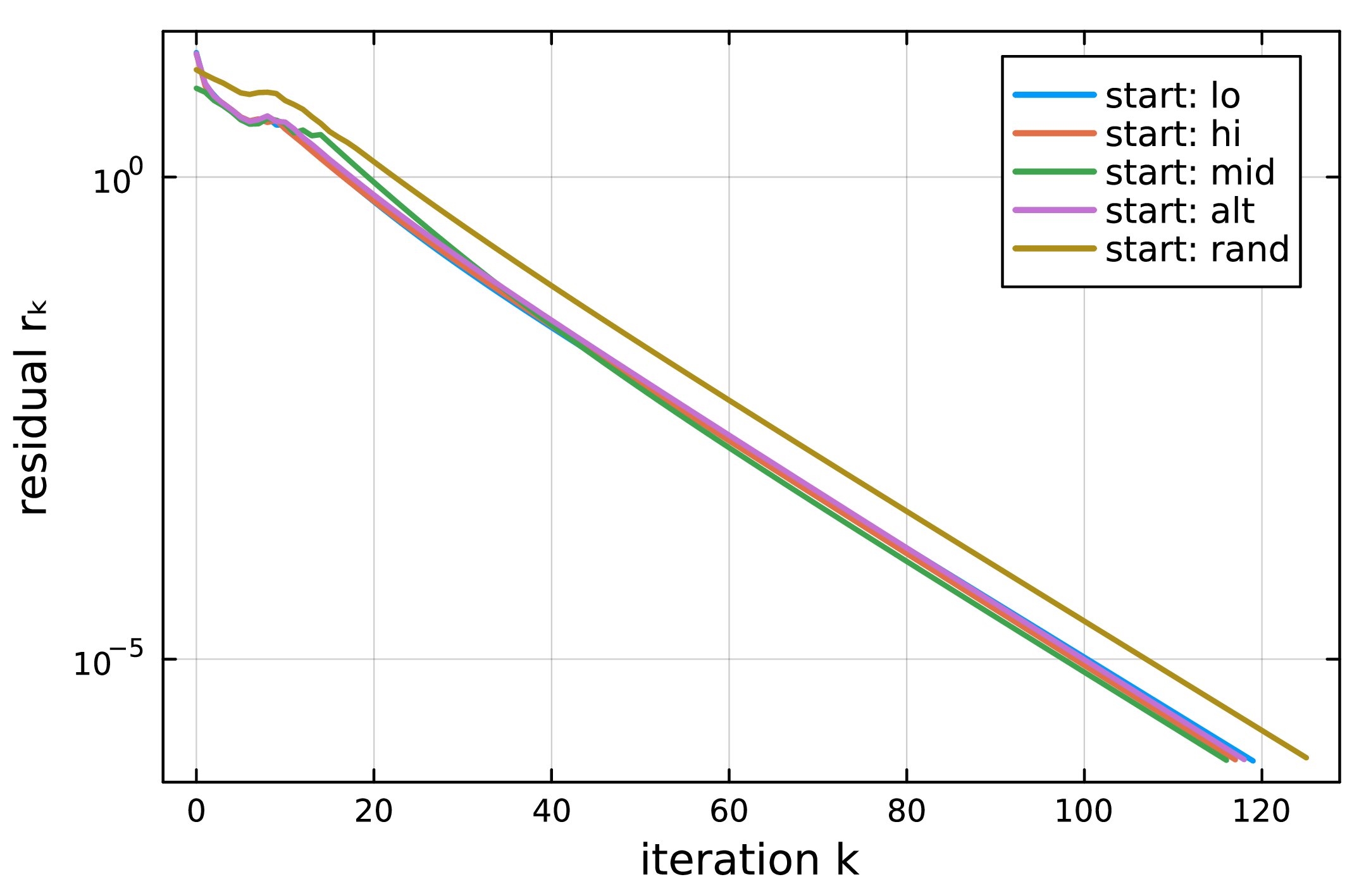
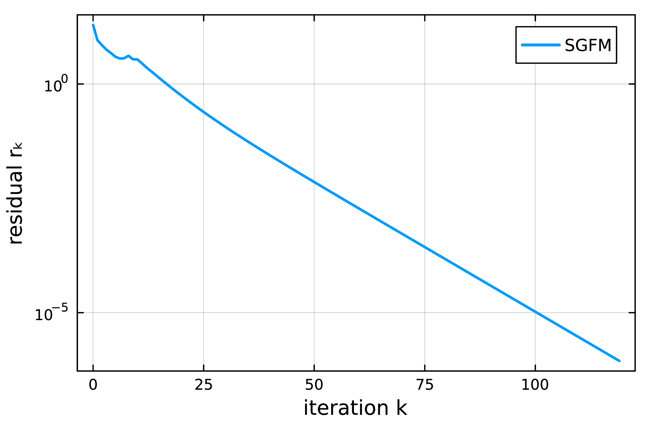
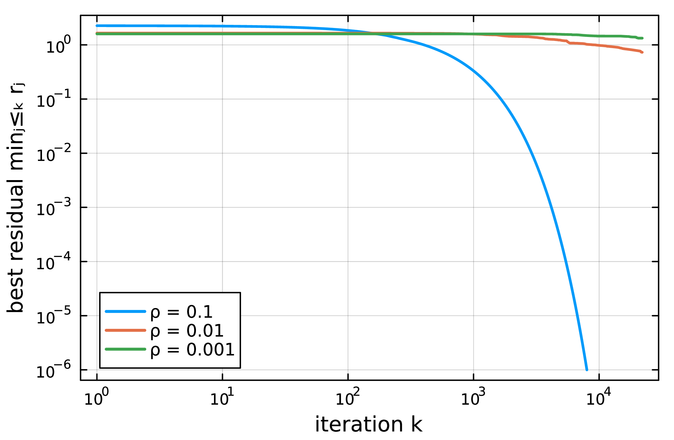
6.6 The variable metric↩︎
On a badly conditioned operator the metric decides the speed, and the diagonal metric wins when the conditioning lies on the diagonal. Figure 5 runs SGFM with the diagonal \(\mathcal{D}_k\) and with \(\mathcal{D}_k=I\) on the affine operator conditioned at \(10^3\). Both residuals are straight lines, so both converge R-linearly as Theorem 19 guarantees, but the diagonal metric reaches \(10^{-6}\) in about \(150\) iterations against about \(1300\) for the Euclidean step, almost ten times fewer. The diagonal metric rescales each coordinate by its own curvature, so the method sees a much smaller effective conditioning. The size of the gain therefore depends on where the ill-conditioning sits. A diagonal metric removes conditioning carried on the diagonal of the operator and cannot touch conditioning carried by the off-diagonal coupling. This is why it helps so much here, where the conditioning is diagonal by construction, and why a projection method slows on problems whose difficulty is rotational instead.
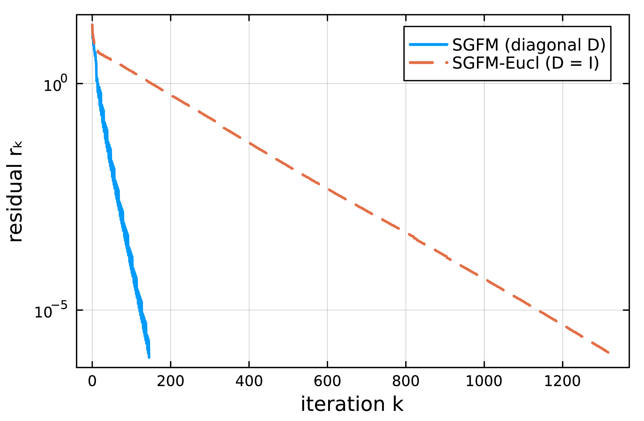
6.7 The modified non-monotone line search↩︎
On these smooth strongly monotone problems the non-monotone line search neither speeds the method up nor slows it down, as the construction predicts. Figure 6 runs SGFM and its monotone version (\(\eta=0\)) on the affine operator, and the two residual curves lie on top of each other. Figure 7 shows the reason. The reference value \(T_k\) stays equal to the gap \(g_\alpha(x_k)\) because the gap already falls at every step, so the relaxation in the Armijo test is never triggered. The non-monotone terms come into play only when a step would raise the gap, and a smooth strongly monotone operator never forces that. The experiment thus measures the cost of the modification and finds it negligible, leaving the relaxation available for the non-monotone problems it is designed for.
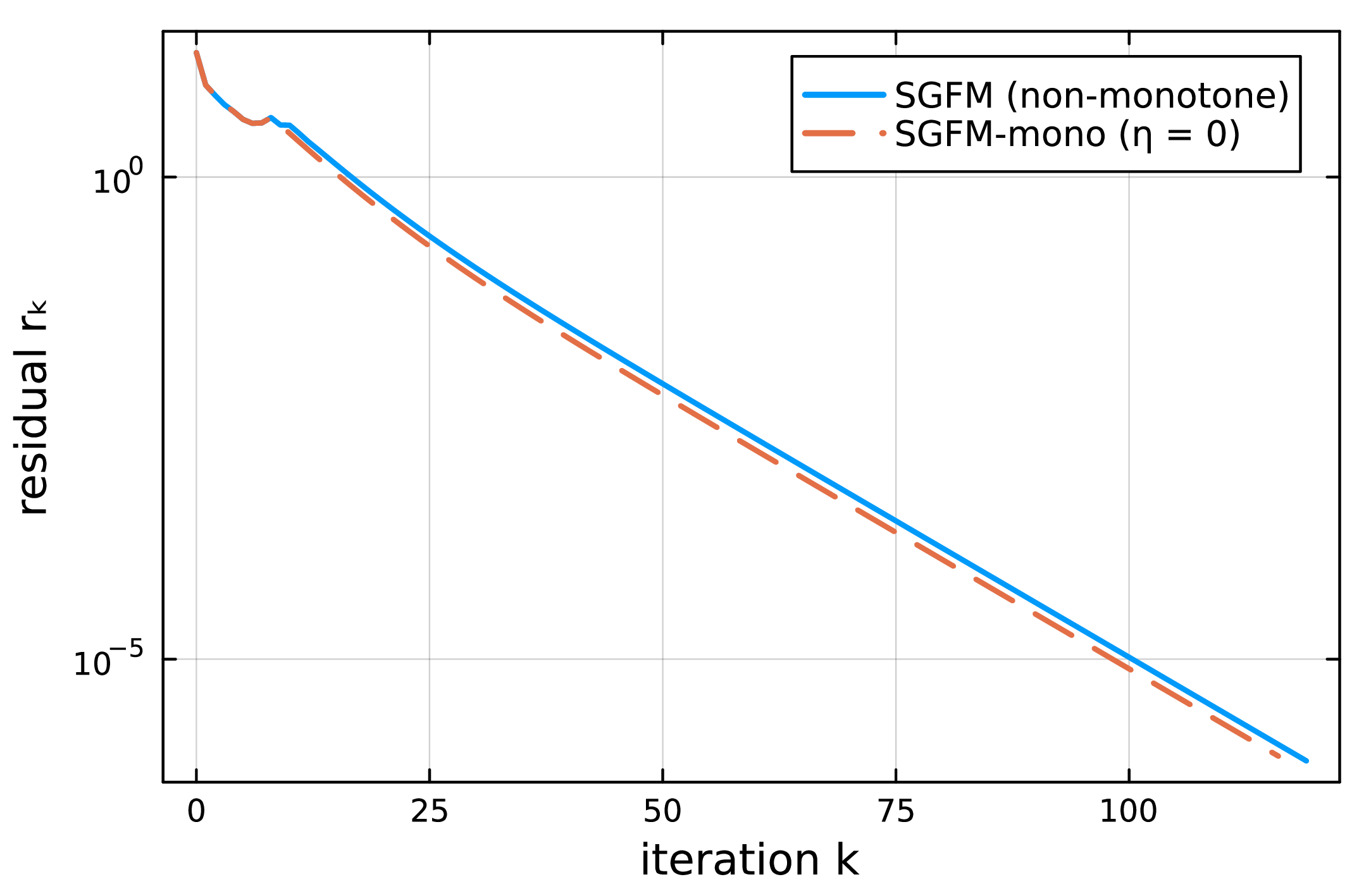
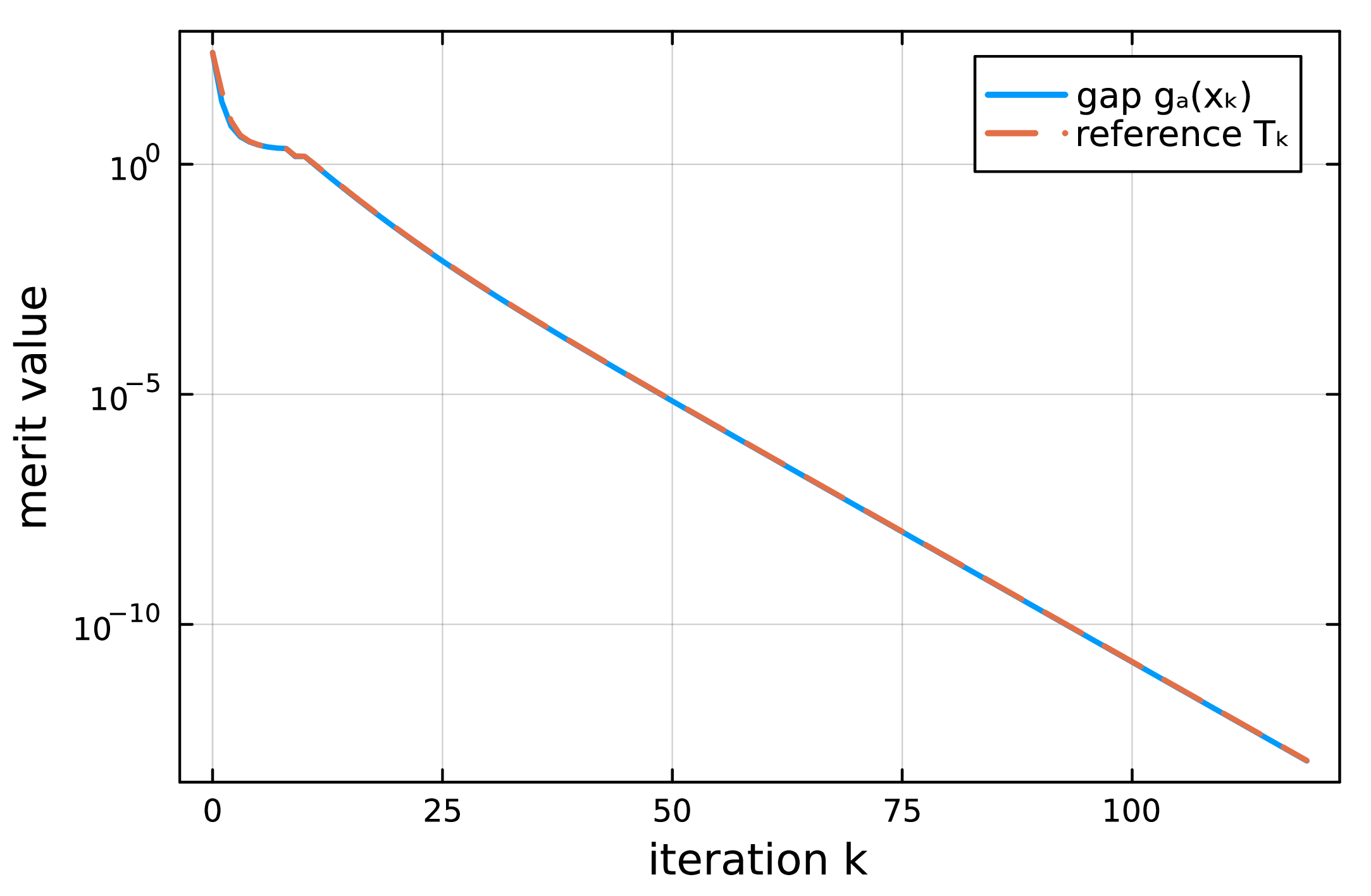
6.8 Merit equivalence↩︎
The gap and the D-gap measure progress in the same way. Figure 8 runs SGFM, which reduces the gap \(g_\alpha\), and the method of Bigi and Passacantando, which reduces the D-gap, on the strongly monotone equilibrium problem (Problem 6). Both merit values fall to zero as straight lines, so both vanish R-linearly. The two slopes differ because the gap and the D-gap agree only up to constant factors (Proposition 18), not because one method is faster than the other. The consequence for the comparison is that the gap we stop on and the D-gap the competitor stops on track the same quantity, so the two methods are measured on common ground.
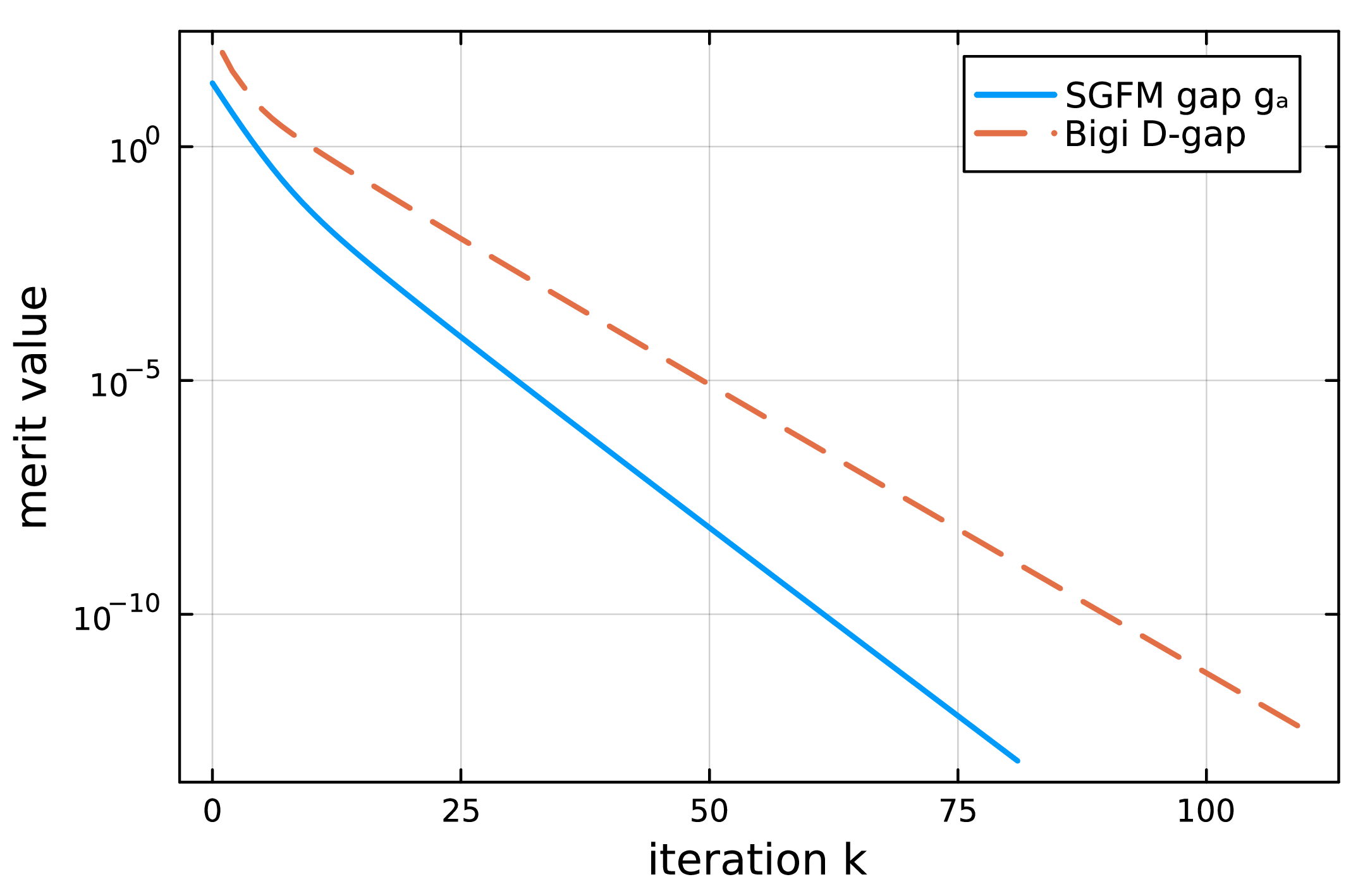
6.9 Comparison with standard methods↩︎
SGFM is on par with the specialized methods on the equilibrium and mixed problems and is slower than the extragradient method on the variational ones. Tables 4 and 5 give the median over the five starts.
On the variational problems (Table 4) the extragradient method is the faster solver, and the gap between the two grows as the operator weakens. On the well-conditioned strongly monotone instance the counts are close, \(94\) iterations for the extragradient method against \(118\) for SGFM. On the weakly monotone instance the extragradient method needs \(157\) iterations and SGFM needs about \(8000\), because the extragradient step stays effective as the modulus \(m\) shrinks while the SGFM rate falls off with \(m\), as Figure 4 already showed. On the non-monotone Kojima–Shindo problem SGFM does not reach the tolerance, while the extragradient method reaches one of the problem’s several solutions. Both results follow the theory. SGFM rests on a strong-monotonicity contraction, and the extragradient method is built for plain monotone and some non-monotone operators.
On the equilibrium problems (Table 5) SGFM is even with the specialized methods where its theory applies. On the strongly monotone instance SGFM and Mastroeni’s gap descent both converge in \(81\) iterations and the D-gap method in \(110\). Mastroeni’s method uses fewer operator evaluations, \(163\) against \(326\), because SGFM does more work per step in its inner solve and line search, so equal iteration counts do not mean equal cost. On the merely monotone Nash–Cournot instance only the D-gap method converges, the regime it was designed for. On the mixed problem SGFM solves the \(\ell_1\)-regularized instance in \(73\) iterations using the fixed relaxation step in place of the line search.
SGFM is not the fastest method on any single class, and the comparison does not aim to make it one. Each competitor is specialized to a single class and tuned for it. What the experiments show is that one method, carrying one analysis, gives the proved guarantees across all three classes: global convergence and the R-linear rate under strong monotonicity, the same rate under the variable metric, and the gap error bound. The price of that reach is the per-iteration work of the gap-based step, and on the variational problems a higher iteration count than a method built for them alone.
| 4-6 Problem | Method | Conv. | Iter. | Op.evals | \(\norm{x-x^*}\) | ||||||||
| Problem [prob:affine] | SGFM | /5 | \(2.0\!\times\!10^{-7}\) | ||||||||||
| EG | /5 | \(2.8\!\times\!10^{-7}\) | |||||||||||
| SGFM | /5 | — | — | — | |||||||||
| EG | /5 | ||||||||||||
| SGFM | /5 | \(1.6\!\times\!10^{-6}\) | |||||||||||
| EG | /5 | \(9.3\!\times\!10^{-6}\) | |||||||||||
| SGFM-MVI | /5 | — |
| 4-6 Problem | Method | Conv. | Iter. | Op.evals | \(\norm{x-x^*}\) | ||||||||
| Problem [prob:cournot] | SGFM | /5 | — | — | — | ||||||||
| MAS | /5 | — | — | — | |||||||||
| Bigi | /5 | — | |||||||||||
| SGFM | /5 | \(2.6\!\times\!10^{-7}\) | |||||||||||
| MAS | /5 | \(2.7\!\times\!10^{-7}\) | |||||||||||
| Bigi | /5 | \(2.6\!\times\!10^{-7}\) |
7 Conclusion↩︎
We extended the scaled gradient modified non-monotone line search method of Ansari et al. [9] from optimization to variational inequalities, mixed variational inequalities, and equilibrium problems, through a gap-function formulation in which the scaled projection coincides with the gap-defining maximizer. For variational and mixed variational inequalities with a strongly monotone Lipschitz operator the analysis yields global convergence and an R-linear rate via a gap error bound, under a fixed or a controlled-change variable metric. For equilibrium problems it yields global convergence and an error bound, with the R-linear rate reduced to such a bound and left open. The numerical experiments confirm these guarantees on controlled problems. The residual contracts R-linearly under strong monotonicity, the diagonal metric is about an order of magnitude faster on ill-conditioned operators, and the method converges from every start across all three classes. Against specialized methods SGFM is competitive on the equilibrium and mixed problems and slower than the extragradient method on the variational ones, the price of a single framework that covers all three.
Several questions are left open, each flagged in the analysis. The first is the equilibrium rate. The Mastroeni-gap error bound of Theorem 23 controls the distance to the solution but is only first order in the residual, so a geometric rate is not automatic. It would follow from a contraction of the auxiliary-equilibrium map under a Lipschitz-type condition on \(G\), once the conflicting requirements on \(\alpha\) are reconciled—the error bound needs \(\alpha\) large, a contraction typically small (Remark 25). The second is the pseudomonotone and nonsmooth range. When the operator is merely pseudomonotone or the data nonsmooth, the smooth-gap descent identity fails, and the line search moves from the gap certificate (V1) to a separating-hyperplane test on the natural residual (V2), carrying the non-monotone reference onto the residual rather than the gap (Remark 26). The third is the strongly quasiconvex class of the base method: because the gap does not inherit strong quasiconvexity (Remark 8), an R-linear rate there must come from a gap error bound derived directly from strong quasiconvexity of \(G(x,\cdot)\). Extensions to quasi-variational inequalities and to a Hilbert-space setting, where the contraction and error-bound arguments use no compactness, are longer-term.
Declarations↩︎
Conflict of interest: The author declares that he has no conflict of interest.
Data Availability↩︎
The Julia code implementing the method, the competitor solvers, the test problems of Section 6.3, and the scripts that generate the tables and figures of Section 6, together with the generated benchmark data, are available from the author on reasonable request and will be released in a public repository upon acceptance. Because every test problem is specified in full in the manuscript, all experiments are reproducible from the stated data.
Funding↩︎
This research did not receive any specific grant from funding agencies in the public, commercial, or not-for-profit sectors. (Funding not applicable).
AI Use Declaration↩︎
During the preparation of this work the author used Claude (Anthropic) to assist with manuscript editing, including tightening prose, verifying LaTeX formatting, and checking internal consistency of cross-references and notation. After using this tool, the author reviewed and edited the content as needed and takes full responsibility for the content of the publication.
Acknowledgment↩︎
The author gratefully acknowledges the support provided by King Fahd University of Petroleum & Minerals (KFUPM) and its Interdisciplinary Research Center (IRC) for Smart Mobility and Logistics.