Hierarchical Logical Processor on the Rotated Surface Code with Shuttle Buses
June 21, 2026
Abstract
Quantum platforms with beyond-planar connectivity provide new opportunities for fault-tolerant quantum computation (FTQC). While quantum low-density parity-check (qLDPC) codes offer high encoding efficiency, their direct implementation requires non-local couplings in every round of syndrome extraction, incurring additional physical error and implementation complexity. To reduce the frequency of such couplings, we propose the Hierarchical Logical Processor (HLP), which concatenates a high-rate quantum CSS code with the rotated surface code (RSC). HLPs can achieve beyond-RSC encoding efficiency while requiring long-range connectivity only once every \(\Theta(d_0)\) rounds of level-0 error correction, where \(d_0\) denotes the base-code distance, substantially reducing the frequency of non-local couplings relative to direct implementations of qLDPC codes. HLPs introduce elongated RSC patches called shuttle buses. Using transversal hybrid-unit CNOT gates, a single shuttle bus can simultaneously couple to multiple standard RSC patches. This capability enables efficient level-1 syndrome extraction with suppressed level-1 error correlations and supports highly parallel logical Pauli measurements. We perform circuit-level simulations of several concrete HLP constructions and benchmark both logical memory and logical Pauli measurement performance. At a physical error rate of \(10^{-3}\), an HLP based on the [[256,194,4]] code achieves \(3\) \(4\) times higher qubit efficiency than the standard RSC. Compared with the yoked surface code [1] on the same level-1 code, this HLP reduces the space overhead per logical qubit by 100200 physical qubits and shortens the logical error-correction cycle time by a factor of 2030.
Utility-scale quantum algorithms require quantum operations at extremely low error rates that are orders of magnitude lower than state-of-the-art error rates on physical qubits [2]–[4]. Fault-tolerant quantum computation (FTQC) aims to bridge this gap between the desired error rate and physical error rates by encoding logical quantum information into quantum error correction (QEC) codes. The rotated surface code (RSC) is a leading QEC code candidate for experimental implementation, since the RSC has simple stabilizer patterns and a high threshold [5], [6]. However, a marked shortcoming of the RSC is its low qubit efficiencya single patch of distance-\(d\) RSC encodes only one logical qubit with \(d^2\) physical qubits. Recent constructions of quantum low-density parity-check (qLDPC) codes [7], [8], such as bivariate bicycle codes [9]–[11], tile codes [12]–[14], hypergraph product codes [15], [16], and lifted product codes [17], [18], offer significantly higher encoding efficiency than the RSC. Direct implementations of qLDPC codes generally require non-local couplings in each round of syndrome extraction (SE), with the required coupling range depending on the specific code construction.
Reconfigurable neutral atom arrays, a rapidly evolving quantum platform supporting long-range connectivity [19]–[21], are promising for realizing these qLDPC codes. Nevertheless, long-range gates, implemented via atom shuttling, can introduce additional physical errors and implementation complexity [19], [20]. Thus, an important consideration is to reduce qubit overhead while limiting the use of long-range gates. For instance, measuring only a fraction of stabilizer generators in each SE round is an effective approach to mitigate the cost of long-range connectivity for implementing qLDPC codes [22]–[24]. A few recent protocols propose using native \(\mathrm{iSWAP}\) gates on superconducting platforms [25]–[27] to extract syndromes and perform routing simultaneously, thereby compiling the code-specific non-local dataancilla connectivity of certain qLDPC codes into SE circuits with only nearest-neighbor coupling [28]–[30]. Alternatively, code concatenationconcatenating a level-1 QEC code on top of a level-0 RSC [1], [31]allows a long time window for measuring non-local level-1 stabilizers, thereby amortizing the demand on non-local connectivity. In particular, a recently proposed quantum memory architecture, yoked surface codes [1], implements specific high-rate level-1 codes on the RSC with only nearest-neighbor connectivity and achieves a three-times higher qubit efficiency compared to the RSC. These recent developments demonstrate promising routes toward high-rate quantum memories under restricted connectivity, while motivating the exploration of logical operations under similar hardware constraints.
In this work, we propose a new FTQC architecture, the hierarchical logical processor (HLP), which implements a high-rate quantum CSS code concatenated with the RSC. HLPs, based on light-weight ancilla patches and transversal CNOT gates, can combine high encoding efficiency with infrequent use of long-range gates and support parallel logical measurements. The key mechanism underlying HLPs is a type of transversal CNOT gate, called the hybrid-unit CNOT gate, that couples an elongated RSC patch (a shuttle bus) to multiple RSC patches (cores) simultaneously. In HLPs, cores and shuttle buses function as level-1 data and ancilla qubits, respectively. We design transversal-CNOT-based readout gadgets, capable of measuring long level-1 Pauli \(\mathsf{X}\) or \(\mathsf{Z}\) operators using only a single shuttle bus. By concurrently using multiple readout gadgets, we can perform level-1 SE substantially faster and with smaller qubit overhead compared with yoked surface codes [1]. We validate our constructions by both theoretical analysis and circuit-level simulations.
Extending beyond logical memory, we propose logical measurement sequences, each composed of a series of readout gadgets, to reliably measure logical Pauli \(X\) or \(Z\) operators. Readout gadgets from different logical measurement sequences can be densely packed to allow parallel measurements of multiple logical operators at the cost of increased use of shuttle buses and non-local transversal CNOT gates. We prove that this protocol achieves full level-1 distance and benchmark it with circuit-level simulations. Additionally, we propose two extension modules that can further enhance the logical functionality of HLPs. First, we propose \(H\)-transformed and \(HS\)-transformed readout gadgets for general logical Pauli measurements. Second, we extend the hybrid-unit CNOT gates to enable joint measurements of logical operators on an HLP and external RSC patches. With relaxed requirements on long-range connectivity, beyond-RSC encoding efficiency, and parallel logical measurement capability, the HLP provides a promising building block for large-scale FTQC architectures.
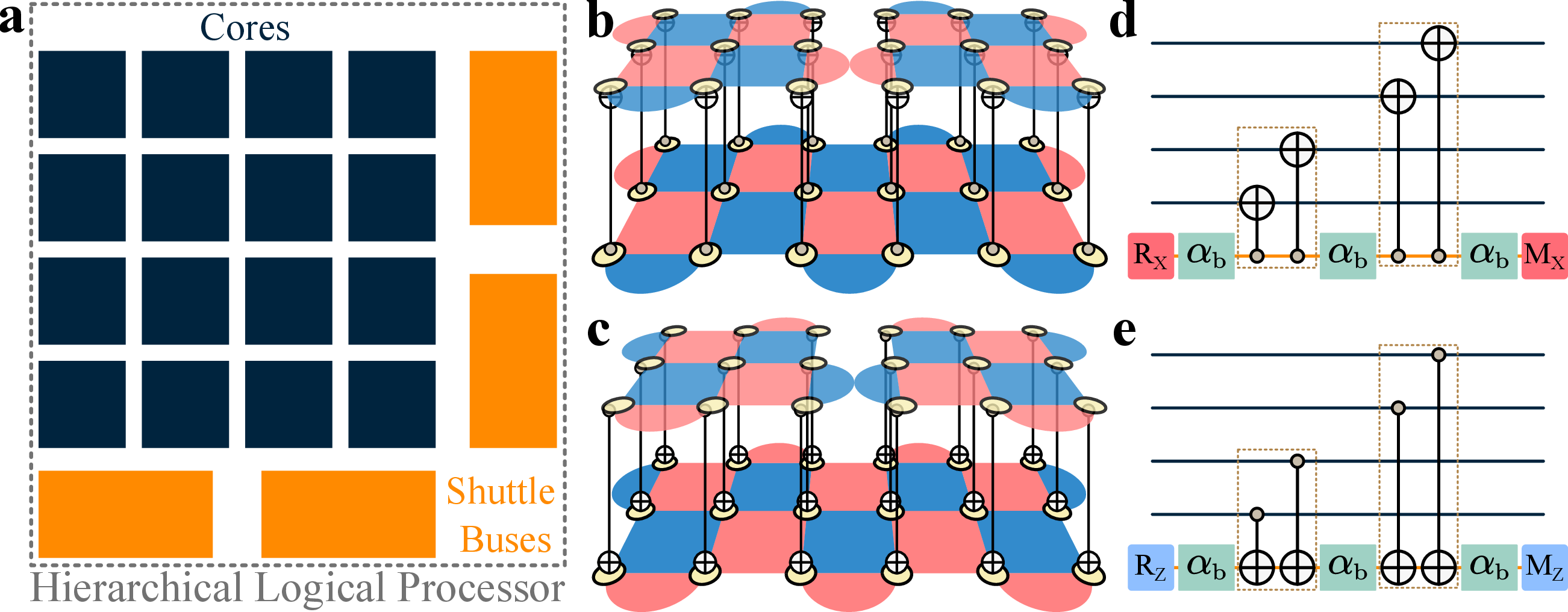
Consider an HLP implementing a distance-\(d_{1}\) level-1 CSS code \(\mathcal{C}_1\) concatenated with the distance-\(d_{0}\) RSC (the level-0 code). The HLP is supported on two types of working units: cores and shuttle buses (Fig. 1 (a)). Each core is a distance-\(d_{0}\) RSC patch, serving as a level-1 data qubit for \(\mathcal{C}_1\); each shuttle bus is an elongated RSC patch of width \(d_{0}\) and length \(d_{0}d_{1}\). A shuttle bus whose logical \(X\) (or \(Z\)) operator runs along the long edge is called an \(X\) (or \(Z\)) bus. We can perform a transversal CNOT gate with a single \(X\) bus on the control side and up to \(d_{1}\) cores on the target side (Fig. 1 (b)). Similarly, we can perform a transversal CNOT gate with up to \(d_{1}\) cores on the control side and a single \(Z\) bus on the target side (Fig. 1 (c)). We refer to the first and the second types of transversal CNOT gates as bus-core and core-bus CNOT gates, respectively. We refer to them collectively as hybrid-unit CNOT gates. With an \(X\) (or \(Z\)) bus as a level-1 ancilla qubit, an \(X\)-basis (or Z-basis) readout gadget can measure a level-1 Pauli \(X\) (or \(Z\)) operator using core-bus (or bus-core) CNOT gates as shown in Fig. 1 (de). We perform level-1 SE on an HLP by extracting level-1 stabilizers with these readout gadgets.
We first consider basic requirements on readout gadgets and their arrangements for running level-1 SE. For every \(X\)-basis readout gadget, \(X\) errors on the \(X\) bus can propagate to multiple cores through bus-core CNOT gates, thereby inducing correlated errors on cores, which would deteriorate the performance of level-1 SE. We note that an \(X\) bus with an \(X\)-basis distance of \(d_{0}d_1\) already strongly suppresses logical \(X\) errors on the bus, which directly induce level-1 hook errors on cores. We insert at least \(\alpha_{\mathsf{b}}d_{0}\) level-0 SE rounds on the \(X\) bus between its initialization (or measurement) and the first (or last) core-bus CNOT gate, and at least \(\alpha_{\mathsf{b}}d_{0}\) level-0 SE rounds between every two adjacent core-bus CNOT gates to limit the propagation speed of \(X\) errors on the bus (Fig. 1). Here, the parameter \(\alpha_{\mathsf{b}}\) depends on \(d_{1}\). Similarly, \(Z\) errors on cores can propagate to multiple \(X\) buses through bus-core CNOT gates, thereby inducing correlated readout errors on these \(X\)-basis readout gadgets. Define the separation between two bus-core CNOT gates as the minimum number of padded level-0 SE rounds between them on every working unit acted on by both of them. Define the separation between two \(X\)-basis readout gadgets as the minimum separation between every pair of bus-core CNOT gates from each gadget. We require every two \(X\)-basis readout gadgets to be separated by at least \(\alpha_{\mathsf{c}}d_{0}\) SE rounds. The same argument applies to \(Z\)-basis gadgets, for which we set the same constraints as above. We refer to \(\alpha_{\mathsf{b}}\) and \(\alpha_{\mathsf{c}}\) as compilation parameters. For simplicity, we restrict to HLPs with perfect time boundaries: all level-0 and level-1 stabilizers are measured perfectly at initialization and final measurement. Thus, cores have perfect time boundaries, whereas shuttle buses are still initialized and measured transversally. We prove (under a phenomenological noise model) that by setting \(\alpha_{\mathsf{b}}=d_{1}\) and \(\alpha_{\mathsf{c}}=1\), we can effectively suppress level-1 error correlations. See the Supplementary Information for the formal theorem statement and proof.
Theorem 1 (Approximate error reduction; informal version of Theorem 2). Consider a circuit composed of level-0 SE rounds on cores and shuttle buses and X- and \(Z\)-basis readout gadgets. Set compilation parameters to \(\alpha_{\mathsf{b}}=d_1\) and \(\alpha_{\mathsf{c}}=1\), and assume perfect time boundaries for cores. Then, under the phenomenological depolarizing noise model with a sufficiently small error rate \(p\), except for a rare event of probability \(\sim p^{d_{0}d_{1}/2}\), the induced level-1 \(X\) (or \(Z\)) errors are local stochastic with an effective level-1 error rate \(p_1\sim p^{d_{0}/2}\); that is, for every level-1 \(X\) (or \(Z\)) error configuration \(\mathsf{f}\), the probability of inducing \(\mathsf{f}\) is upper bounded by \(\sim p_1^{|\mathsf{f}|}\).
The compilation parameter \(\alpha_{\mathsf{b}}\) characterizes the sparsity of hybrid-unit CNOT gates on every shuttle bus. In other words, a layer of long-range physical CNOT gates is required at most once per \(\alpha_{\mathsf{b}} d_{0}\) level-0 SE rounds for every shuttle bus. Similarly, the compilation parameter \(\alpha_{\mathsf{c}}\) characterizes the sparsity of core-bus (or bus-core) CNOT gates on a core. We can also make a stronger requirement that every two readout gadgets (regardless of their basis) should be separated by at least \(\alpha_{\mathsf{c}}d_{0}\) level-0 SE rounds. (All level-1 SE circuits for our concrete HLP constructions in the following satisfy this constraint.) In this way, long-range CNOT gates are required only once per \(\Theta(d_{0})\) level-0 SE rounds for every working unit. We note that larger compilation parameters relax the demand on long-range connectivity at the cost of longer level-1 SE round time, which serves as the fundamental timescale for logical operations. Thus, we would like to minimize compilation parameters as long as (i) the level-1 \(X\) (or \(Z\)) errors are still effectively uncorrelated, and (ii) the hardware can keep up with the required long-range connectivity.
![Figure 2: Benchmarking the memory performance of various hierarchical logical processors (HLP). (a) Level-1 layout of an HLP based on the [[64,34,4]] Square Berg code [1]. Cores (level-1 data qubits) and shuttle buses (level-1 ancilla qubits) are represented by dark squares and orange rectangles, respectively. Each Level-1 X (or Z) stabilizer is shown as a red (or blue) circle and is connected to all level-1 data qubits on its support by red (or blue) lines. (b) Circuit-level simulations of two HLPs based on the [[4,2,2]] Iceberg code and the [[64,34,4]] Square Berg code, respectively. We fix \alpha_{\mathsf{c}}=1. The first HLP is operated under either \alpha_{\mathsf{b}}=0.5 or \alpha_{\mathsf{b}}=1. The second HLP is operated under \alpha_{\mathsf{b}}=1. We also perform soft-output simulations of both HLPs with \alpha_{\mathsf{b}}=1. (cd) Extrapolated qubit overhead and level-1 SE round time for the RSC, HLPs, and a yoked surface code [1]. The HLP based on the [[10,8,2]] Iceberg code uses a single shuttle bus at a time as in (b); the HLP based on the [[16,14,2]] Iceberg code uses two shuttle buses to extract both level-1 X and Z stabilizers in parallel. The HLP based on the [[256,194,4]] Square Berg code uses 16 shuttle buses in a similar way to (a). The yoked surface code is based on the same Square Berg code. The level-1 time for the RSC baseline in (d) is set as d level-0 SE rounds for a distance-d RSC. All numerical results are obtained assuming (i) the circuit-level uniform depolarizing noise model with a physical error rate of 10^{-3} and (ii) perfect time boundaries for HLPs.](/article/2606.22594/figs/hlp_performance_main.png "fig:")
A Level-1 memory circuit on an HLP is implemented by a level-0 circuit, consisting of level-0 SE on all working units, transversal initialization and measurement on shuttle buses, and hybrid-unit CNOT gates. The level-0 circuit generates level-0 detectors (composed of level-0 stabilizer measurements from at most two adjacent level-0 SE rounds); the level-1 memory circuit generates level-1 detectors corresponding to measurement results of level-1 stabilizers in two adjacent level-1 SE rounds. To decode the level-1 memory circuit, we first perform a matching-based level-0 decoding on level-0 detectors, which amounts to decoding circuits on the RSC (and the elongated RSC) with level-0 SE rounds interleaved by structured transversal CNOT gates [32]–[38]; we then extract soft outputs [39] from segments of the level-0 decoding graphs on cores and shuttle buses, such that each soft output estimates the error probability at the corresponding level-1 error location; finally, we perform level-1 decoding on level-1 detectors, with level-1 error probabilities informed by soft outputs.
We benchmark the memory performance of our HLP design with two types of matchable level-1 codes, the Iceberg code and the 2D parity check code, following Ref. [1]. We refer to the latter as the Square Berg code in the following to avoid confusion with qLDPC codes. We fix \(\alpha_{\mathsf{c}}=1\) in our numerical simulations. We perform circuit-level simulation of (i) an HLP with the \([[4,2,2]]\) Iceberg code as its level-1 code and (ii) an HLP with the \([[64,34,4]]\) Square Berg code (Fig. 2 (a)) as its level-1 code under the circuit-level uniform depolarizing noise model with a physical error rate of \(10^{-3}\). The first HLP extracts the level-1 \(X\) and \(Z\) stabilizers sequentially in a level-1 SE round. We observe that, under both compilation-parameter settings \(\alpha_{\mathsf{b}}=0.5\) and \(\alpha_{\mathsf{b}}=1\), the logical error rate (LER) decays with increasing core distance at nearly twice the rate observed for the RSC. The second HLP on the \([[64,34,4]]\) Square Berg code uses eight concurrent shuttle buses to extract level-1 stabilizers in parallel (Fig. 2 (a)). Its LER decays with increasing core distance at approximately twice the rate observed for the first HLP. These circuit-level simulations indicate that both HLPs operate close to their full distance \(d_{0}d_{1}\). We develop a high-speed heuristic simulator, the soft-output simulator (similar to the gap simulator in Ref. [1]), that directly samples errors and performs decoding at level 1, thereby enabling fast benchmarking of large-scale HLPs. We find close agreement between the soft-output and circuit-level simulation results (Fig. 2 (b)). With the soft-output simulator, we perform level-1 simulation on HLPs with even larger level-1 code sizes and extrapolate their memory performance. We see that with the \([[256,194,4]]\) Square Berg code as the level-1 code, our HLP (now with sixteen concurrent shuttle buses) has a three to four times higher qubit efficiency compared to the RSC over a wide range of target logical error rates, from \(10^{-10}\) to \(10^{-15}\). Compared to the yoked surface code [1] with the same level-1 code and circuit-level noise model, our HLP offers a reduction of 100200 physical qubits in space overhead per logical qubit and a \(20\) \(30\)-fold reduction in level-1 SE round time at similar target logical error rates. See the Supplementary Information for details on circuit-level and soft-out simulations. We note that our HLP on the \([[256,194,4]]\) Square Berg code still has roughly ten times larger level-1 SE round time compared to the RSC baseline set as \(d\) level-0 SE rounds for a distance-\(d\) RSC. This round time sets a lower bound on the latency for logical feedforward operations. However, the logical processing speed also depends on the logical circuit at hand and the parallelism of logical operations. We now show how logical Pauli measurements can be performed in parallel on an HLP.
![Figure 3: Logical Pauli measurements on a hierarchical logical processor (HLP). (a) A Z-basis logical measurement sequence of d_{1} logical readout gadgets, in d_1 consecutive level-1 syndrome extraction (SE) rounds; each logical readout gadget is embedded in a distinct level-1 SE round. (b) Dense packing of logical readout gadgets from different logical measurement sequences targeting logical Pauli Z operators \mathsf{P}_{1}, \mathsf{P}_2, and \mathsf{P}_3, respectively. Each teal strip on the core represents a single level-0 SE round. (c) Performance of logical Z measurements on an HLP whose level-1 code is the [[8,6,2]] Iceberg code. The memory baseline is composed of five level-1 SE rounds with perfect time boundaries. Logical error rates (LERs) accounting for both logical measurement errors and memory errors are shown as squares; LERs for logical measurement errors alone are shown as hexagons. (d) H-transformed readout gadget for measuring a logical Pauli operator \mathsf{P}_{xz} with x\cdot z=0. (e) HS-transformed readout gadget for measuring a logical Pauli operator \mathsf{P}_{xz} with x\cdot z=1. (f) Extended core-bus CNOT gate between an external core and a Z bus.](/article/2606.22594/figs/hlp_logical_measurements_main.png "fig:")
We use a sequence of \(X\)-basis (or \(Z\)-basis) readout gadgets to reliably measure a logical Pauli \(X\) (or \(Z\)) operator. We call such a sequence a logical measurement sequence (LMS), and call the readout gadgets in an LMS logical readout gadgets. More specifically, an LMS consists of \(d_{1}\) logical readout gadgets embedded in \(d_{1}\) consecutive level-1 SE rounds, such that each level-1 SE round contains exactly one logical readout gadget (Fig. 3 (a)). Every pair of adjacent logical readout gadgets in an LMS generates an additional level-1 detector to check for readout errors on either gadget. We refer to an LMS based on \(X\)-basis (or \(Z\)-basis) logical readout gadgets as an \(X\)-basis (or \(Z\)-basis) LMS. We require each \(X\)-basis (or \(Z\)-basis) logical readout gadget in an \(X\)-basis (or \(Z\)-basis) LMS to be separated by at least \(\alpha_{\mathsf{c}} d_{0}\) level-0 SE rounds from both the other logical readout gadgets in the same LMS and \(X\)-basis (or \(Z\)-basis) readout gadgets for level-1 SE, so as to suppress correlations among readout errors on these gadgets. When it comes to measuring multiple logical Pauli \(X\) or \(Z\) operators, we can perform level-1 decoding for each LMS independently, based on the level-1 detectors from level-1 SE and the level-1 detectors generated by this LMS. Moreover, we do not need to suppress error correlation between readout errors on logical readout gadgets in different LMSs. Therefore, the separation between each pair of logical readout gadgets from two different LMSs can be as small as one level-0 SE round (Fig. 3 (b)). This allows dense packing of logical readout gadgets from different LMSs inside a level-1 SE round, thereby enabling high parallelism in logical operations at the cost of increased use of ancillary shuttle buses and long-range CNOT gates.
We benchmark logical Pauli measurements on an HLP using the \([[8,6,2]]\) Iceberg code as the level-1 code. We label level-1 data qubits of the code by \(\{1,\cdots,8\}\) and logical qubits by \(\{1,\cdots,6\}\). We choose the logical \(Z\) operator for the \(i\)th logical qubit according to \(\overline{\mathsf{Z}}_{i}:=\mathsf{Z}_{i+1}\otimes\mathsf{Z}_{8}\). Consider the following three logical \(Z\) operators \(\mathsf{Z}_2\otimes\mathsf{Z}_{3}\otimes\cdots\otimes\mathsf{Z}_{7}\), equivalently \(\overline{\mathsf{Z}}_{1}\cdot\overline{\mathsf{Z}}_{2}\cdots\overline{\mathsf{Z}}_{6}\); \(\mathsf{Z}_{2}\otimes\mathsf{Z}_{3}\otimes\mathsf{Z}_{4}\otimes\mathsf{Z}_{8}\), equivalently \(\overline{\mathsf{Z}}_1\cdot\overline{\mathsf{Z}}_2\cdot\overline{\mathsf{Z}}_3\); and \(\mathsf{Z}_{5}\otimes\mathsf{Z}_{6}\otimes\mathsf{Z}_7\otimes\mathsf{Z}_8\), equivalently \(\overline{\mathsf{Z}}_4\cdot\overline{\mathsf{Z}}_5\cdot\overline{\mathsf{Z}}_6\). We examine two circuits, both with five level-1 SE rounds and perfect time boundaries. The first circuit uses a single LMS to measure the first logical \(Z\) operator, whereas the second circuit uses three LMSs to measure the three logical \(Z\) operators listed above. Time boundary conditions for logical operators in both circuits guarantee predetermined LMS outcomes and allow logical errors on unmeasured logical degrees of freedom to be detected; see the Supplementary Information for a detailed description. Moreover, for the second circuit, the separation between logical readout gadgets belonging to different LMSs can be as small as one level-0 SE round. We observe that the presence of LMSs does not appreciably increase the total logical error rate, and that the error rates for LMSs are significantly lower than logical memory error rates. These results demonstrate both (i) the feasibility of using an LMS to measure long logical Pauli operators and (ii) the parallelizability of LMSs.
Now consider measuring a general logical operator \(\mathsf{P}_{xz}:=i^{x\cdot z}\mathsf{X}_{1}^{x_1}\mathsf{Z}_1^{z_1}\otimes \cdots\otimes \mathsf{X}_{n_1}^{x_{n_1}}\mathsf{Z}_{n_1}^{z_{n_1}}\), where \(n_1\) is the number of level-1 data qubits; \(x=(x_1,\cdots,x_{n_1})\) and \(z=(z_{1},\cdots,z_{n_1})\) are both elements in \(\mathbb{Z}_2^{n_1}\). If \(x\cdot z=0\), we propose the \(H\)-transformed gadget (Fig. 3 (d)) to measure \(\mathsf{P}_{xz}\). This gadget starts with a \(Z\) bus and performs core-bus CNOT gates according to the \(Z\) component in \(\mathsf{P}_{xz}\), then switches to an \(X\) bus via a transversal \(H\) gate and performs bus-core CNOT gates according to the \(X\) component in \(\mathsf{P}_{xz}\), and finally measures the bus in \(X\) basis. Due to the close resemblance between the first (or second) half of the \(H\) gadget and a \(Z\)-basis (or \(X\)-basis) readout gadget, we can similarly construct LMSs from \(H\)-transformed gadgets, thereby achieving full level-1 distance for measuring \(\mathsf{P}_{xz}\) and parallelizability comparable to that of LMSs based on \(X\)-basis or \(Z\)-basis readout gadgets. For the \(x\cdot z=1\) case, we can also use the \(H\)-transformed gadget to measure \(\mathsf{P}_{xz}\) given an ancillary logical \(Y\) state (which would remain invariant under the measurement) [40]. To remove the need for this catalytic logical \(Y\) state, we propose the \(HS\)-transformed readout gadget in Fig. 3 (e), where the logical \(S\) gate in the gadget can be performed by a mid-cycle fold transversal gate [25], [41]. Finally, the hybrid-unit CNOT gates between shuttle buses and cores with the same width can be straightforwardly extended to act between shuttle buses and external cores (RSC patches) with distance \(d_{ext}\) satisfying \(d_{0}\leq d_{ext}\leq d_{0}d_{1}\) (see Fig. 3 (f)). This allows a shuttle bus to perform joint logical Pauli measurements involving logical qubits hosted on both an HLP and external cores. We leave numerical benchmarking of these protocols for future work.
To summarize, we design the HLP, a concatenation-based FTQC architecture that can offer beyond-RSC encoding efficiency while using long-range CNOT gates as infrequently as once every \(\Theta(d_0)\) level-0 SE rounds for
each working unit, where \(d_{0}\) is the base RSC distance. The HLP architecture crucially relies on transversal hybrid-unit CNOT gates between cores (RSC patches) and shuttle buses (elongated RSC patches). Leveraging
these hybrid-unit CNOT gates, we design readout gadgets to perform level-1 SE and LMSs to perform logical measurements in parallel. These protocols and our numerical benchmarking serve as a starting point for using HLPs in large-scale FTQC. There is a
broad range of directions for future investigation. First, we expect that the memory overhead can be further lowered by using level-1 codes with higher rates and slightly larger level-1 distances compared to the Square Berg code used here. One may also
consider changing the level-0 code from the RSC to a small qLDPC code and redesigning shuttle buses for it. Recent works on logical operations [42]–[52] and soft-information decoding [53]–[56] for qLDPC codes can help in this new
design. In this way, we may obtain a logical memory architecture achieving utility-scale logical error rates at an encoding rate close to a small qLDPC code with moderate use of long-range connectivitylong-range connectivity for a level-0 SE round should
be at the same scale as the small qLDPC code, and long-range connectivity for level-1 SE should be amortized in time. Secondly, as for logical operations, since a hierarchical structure necessarily leads to longer logical operation timescales, leveraging
the parallelizability of logical measurements and the capability of measuring long logical operators will be important for achieving higher logical processing throughput. Alternative ways to perform logical operations on an HLPsuch as transversal logical
gates at level 1 assisted by level-1 flag qubits [57]–[60]are also worth investigation. Moreover, a careful study is needed to understand how HLPs and external cores can cooperate to solve quantum tasks with high efficiency. Finally,
it is important to consider the hardware implementation of an HLP. For instance, one promising candidate is the local-CZ-based architecture [61]–[63] for neutral atoms, which allows in-place implementation of entangling gates in the level-0 SE without atom
shuttling. It would be interesting to explore whether this architecture offers a significant speedup for our HLP compared to the zone-based architecture [20], [64].
NoteSee the public repository [65] for circuits and source codes used in our numerical experiments.
Related worksAfter completing this manuscript, we became aware of two recent related works [66],
[67]. Ref. [66] studies a hierarchical logical memory
architecture based on concatenating an algebraic code with a qLDPC code, using a bivariate bicycle code as the level-0 code and logical cat states for level-1 syndrome extraction. Ref. [67] introduces ‘dense-packing’, a variant of the surface code with densely packed twist defects, achieving \(2\times\) encoding rate of the rotated surface code.
Ref. [67] further studies the concatenation of Iceberg codes with dense-packing in a similar manner to yoked surface codes [1]. In contrast, our work develops a transversal-gate-based hierarchical logical processor (HLP) architecture built on the rotated surface
code, featuring short level-1 syndrome extraction time (measured in level-0 syndrome extraction rounds) and highly parallel logical measurements. We additionally perform full circuit-level simulations of several concrete HLP constructions. Overall, these
works [66], [67] and ours are largely
complementary: together they explore different hardware assumptions, level-0 code choices, and hierarchical structures toward the common goal of reducing the resource overhead of FTQC with moderate demands on hardware platforms.
Supplemental Material for
“Hierarchical Logical Processor on the Rotated Surface Code with Shuttle Buses”
Zi-Han Chen,\(^{1,2,3,}\) \(\;\)Ming-Cheng Chen,\(^{1,2,3}\) Chao-Yang Lu,\(^{1,2,3}\) and Jian-Wei Pan\(^{1,2,3}\)
\(^{1}\)Hefei National Research Center for Physical Sciences at the Microscale and School of Physical Sciences, University of Science and Technology of China, Hefei 230026, China
\(^{2}\)Shanghai Research Center for Quantum Science and CAS Center for Excellence in Quantum Information and Quantum Physics, University of Science and Technology of China, Shanghai 201315, China
\(^{3}\)Hefei National Laboratory, University of Science and Technology of China, Hefei 230088, China
We present a detailed description of the hierarchical logical processor (HLP) architecture in the supplementary material. In Sec. 1 , we describe basic modules for an HLP and its decoding procedure. In Sec. 2, we analyze the induced level-1 error model from level-0 errors. We prove that the correlation between level-1 \(X\) (or \(Z\)) errors can be effectively suppressed. In Sec. 3, we prove that our logical \(X\) (or \(Z\)) measurement protocol (with an LMS) achieves full level-1 distance. We then upper bound the probability of logical measurement errors for LMSs using the induced level-1 error model analyzed in Sec. 2. We describe the construction of two additional readout gadgets, the \(H\)-transformed readout gadget and the \(HS\)-transformed readout gadget. For LMSs based on \(H\)-transformed readout gadgets, we prove similar results to \(X\)-basis (or \(Z\)-basis) LMSs. We describe the extension of hybrid-unit CNOT gates to enable interfacing an HLP with external cores. In Sec. 4, we describe details on numerical simulations, including circuit-level simulations, soft-output simulations, and logical error rate extrapolation. See the public repository [65] for circuits and source codes used in our numerical experiments.
1 Hierarchical Logical Processor: Basic Modules↩︎
Our HLP essentially implements fault-tolerant logical operations (preserving logical information and measuring logical Pauli operators) on a concatenated codelogical information is encoded in a level-1 high-rate CSS code \(\mathcal{C}_1\) with a distance of \(d_1\), which is run on top of the level-0 distance-\(d_0\) RSC. In this section, we describe key components for our HLP and how to perform level-1 SE and logical Pauli \(X\) or \(Z\) measurements. We describe extensions to these modules, including performing general logical Pauli measurements and interfacing with logical information directly encoded in external RSC patches (external cores), in later sections.
1.1 Cores, shuttle buses, and hybrid-unit CNOT gates↩︎
An HLP consists of two working units: cores and shuttle buses, both of which are code patches whose logical qubits serve as level-1 qubits. Every level-1 data qubit of \(\mathcal{C}_1\) is the logical qubit of a distance-\(d_{0}\) RSC patch, referred to as a core. Every level-1 ancilla qubit for level-1 SE and logical Pauli measurements in our HLP is the logical qubit of an elongated RSC patch, referred to as a shuttle bus. We require each shuttle bus to have a width of \(d_0\) and a length of \(d_0d_1\). We note that our specific choice here is for a clean presentation of results, and that it is possible to use shuttle buses of different widths and lengths. A shuttle bus whose logical \(X\) (or \(Z\)) operator is supported on the long edge is called an \(X\) (or \(Z\)) bus. See Fig. 4 for an illustration of cores, \(X\) buses, and \(Z\) buses. We can perform (with a depth-1 layer of physical CNOT gates) transversal logical CNOT gates with an \(X\) (or \(Z\)) bus on the control side (or target side) and up to \(d_1\) cores on the target side (or control side). We refer to a depth-1 layer of physical CNOT gates implementing logical CNOT gates between (up to \(d_1\)) cores and a shuttle bus as a hybrid-unit CNOT gate. More specifically, a hybrid-unit CNOT gate between an \(X\) (or \(Z\)) bus and up to \(d_1\) cores is called a bus-core (or core-bus) CNOT gate.

1.2 Circuit structure and error model↩︎
Level-0 circuit structureFor conceptual simplicity and hardware friendliness, we implement level-0 SE rounds on cores and shuttle buses synchronously and require that there is at most a depth-1 layer of hybrid-unit CNOT gates between every two consecutive level-0 SE rounds. We refer to each level-0 SE round with its preceding depth-1 layer of hybrid-unit CNOT gates (if any) as a level-0 time step. We now define the (time-like) separation between two hybrid-unit CNOT gates.
Definition 1 (Separation between two hybrid-unit CNOT gates). If the supports of two hybrid-unit CNOT gates are not disjoint, their separation is defined as the absolute difference between their corresponding level-0 time steps. Otherwise, their separation is defined to be infinity.
We merge transversal initialization (or measurement) on a shuttle bus into the following (or preceding) level-0 SE round on the working unit. A shuttle bus is activated by the transversal initialization and deactivated by the transversal measurement. A deactivated shuttle bus will no longer be activated again. Instead, we reallocate all qubits of a deactivated shuttle bus to activate new shuttle buses later. We define the lifetime of a shuttle bus as the period between the level-0 time step at which the shuttle bus is initialized and the level-0 time step at which the shuttle bus is measured.
Level-1 circuit structureEvery level-0 circuit on cores and shuttle buses induces a corresponding level-1 circuit that represents operations on logical qubits of these working units. More specifically, level-0 SE rounds correspond to idling operations at level 1; transversal initialization and measurement on shuttle buses correspond to reset and measurement operations on their corresponding logical qubits at level 1; hybrid-unit CNOT gates correspond to level-1 CNOT gates. In every layer of a level-1 circuit, each level-1 qubit (corresponding to the logical qubit of a working unit) participates in one type of level-1 operation. Since each hybrid-unit CNOT gate can simultaneously couple a level-1 ancilla with up to \(d_1\) level-1 data qubits, we require that in every level-1 layer, (i) every level-1 data qubit participates in at most one CNOT gate with a level-1 ancilla and (ii) every level-1 ancilla qubit on an \(X\) (or \(Z\)) bus participates in at most \(d_1\) CNOT gates on the control side (or target side).
Perfect time boundariesThroughout this work, we consider HLPs with perfect initialization and measurement. More specifically, an HLP is initialized by (i) measuring all level-0 and level-1 stabilizers perfectly and (ii) measuring a collection of logical Pauli operators perfectly according to the logical initialization basis. Similarly, the final measurement on an HLP applies the same perfect measurement procedure used during perfect initialization.
Uniform depolarizing circuit noise modelThis model is a standard circuit-level noise model used for benchmarking fault-tolerant protocols. We perform all numerical simulations on level-0 circuits using this circuit noise model, with error locations listed as follows.
Each single-qubit initialization in \(X\) (or \(Z\)) basis is followed by a single-qubit \(Z\) (or \(X\)) error with probability \(p\).
Each single-qubit measurement in \(X\) (or \(Z\)) basis is preceded by a single-qubit \(Z\) or (\(X\)) error with probability \(p\).
Each single-qubit gate (including idling) is followed by a single-qubit depolarizing channel with noise strength \(p\), consisting of three independent Pauli errors \(\{X,Y,Z\}\), each with probability \(p/3\).
Each two-qubit gate is followed by a two-qubit depolarizing channel with noise strength \(p\), consisting of 15 independent Pauli errors \(\{I,X,Y,Z\}^{\otimes2}\backslash\{II\}\), each with probability \(p/15\).
Each single-qubit measurement result is flipped with probability \(p\).
Phenomenological depolarizing noise modelIn this noise model, errors may only occur on level-0 data qubits at the beginning of each level-0 time step and on level-0 measurement results. We regard an \(X\)-basis (or \(Z\)-basis) measurement error as a \(Z\) (or \(X\)) error. The error locations are listed as follows.
For each working unit \(\sigma\) at the beginning of every level-0 time step, if \(\sigma\) is transversally initialized in the \(X\) (or \(Z\)) basis, then every data qubit of \(\sigma\) experiences a Pauli \(Z\) (or \(X\)) error with probability \(p\) following the transversal initialization. Otherwise, every data qubit experiences a single-qubit depolarizing channel with noise strength \(p\).
Every measurement result is flipped with probability \(p\).
1.3 Level-1 readout gadget↩︎
An \(X\)-basis (or \(Z\)-basis) readout gadget performs a projective measurement on a level-1 Pauli \(X\) (or \(Z\)) operator on level-1 data qubits with a level-1 ancilla implemented by an \(X\) bus (or \(Z\) bus). More specifically, for a level-1 Pauli \(X\) operator \(\mathsf{P}_{x}:=\mathsf{X}_1^{x_1}\otimes\cdots\otimes\mathsf{X}_{n_1}^{x_{n_1}}\) where \(x:=(x_1,\cdots,x_{n_1})\) is a vector in \(\mathbb{Z}_2^{n_1}\), the level-1 circuit of an \(X\)-basis readout gadget to measure \(\mathsf{P}_{x}\) proceeds as follows:
Initialize the level-1 ancilla in the \(X\) basis.
Perform a sequence of CNOT gates between the level-1 ancilla (control) and level-1 data qubits (target), such that for every level-1 data qubit \(i\) with \(x_i=1\), there is exactly one CNOT gate between this level-1 data qubit and the level-1 ancilla. Every level-1 layer of CNOT gates has at most \(d_1\) level-1 data qubits on the target side.
Measure the level-1 ancilla in the \(X\) basis.
Similarly, the level-1 circuit of a \(Z\)-basis readout gadget to measure a level-1 Pauli \(Z\) operator \(\mathsf{P}_z:=\mathsf{Z}_1^{z_1}\otimes\cdots\otimes\mathsf{Z}_{n_1}^{z_{n_1}}\) with \(z:=(z_1,\cdots,z_n)\in\mathbb{Z}_2^{n_1}\) proceeds as follows:
Initialize the level-1 ancilla in the \(Z\) basis.
Perform a sequence of CNOT gates between level-1 data qubits (control) and the level-1 ancilla qubit (target), such that for every level-1 data qubit \(i\) with \(z_i=1\), there is exactly one CNOT gate between this level-1 data qubit and the level-1 ancilla. Every level-1 layer of CNOT gates has at most \(d_1\) level-1 data qubits on the control side.
Measure the level-1 ancilla in the \(Z\) basis.
We now describe the level-0 implementation of an \(X\)-basis (or \(Z\)-basis) readout gadget. The level-1 ancilla of the readout gadget is the logical qubit of the shuttle bus associated with the gadget. Initialization and measurement on the level-1 ancilla in the \(X\) or \(Z\) basis are implemented by transversal initialization and measurement on the corresponding shuttle bus, respectively. Every level-1 layer of CNOT gates in the readout gadget is implemented by a hybrid-unit CNOT gate. We insert padding level-0 SE rounds on the shuttle bus so that (i) every two adjacent hybrid-unit CNOT gates in the readout gadget are separated by at least \(\alpha_{\mathsf{b}}d_{0}\) level-0 SE rounds and (ii) transversal reset (or measurement) of the shuttle bus is separated from the following (or preceding) hybrid-unit CNOT gate by at least \(\alpha_{\mathsf{b}}d_{0}\) rounds. Note that level-0 \(X\) (or \(Z\)) errors on \(X\) (or \(Z\)) buses may propagate to cores via hybrid-unit CNOT gates, thereby inducing correlated errors at level 1. The parameter \(\alpha_{\mathsf{b}}\) should therefore be chosen to suppress such error correlations. Moreover, the level-1 measurement result, referred to as the readout value, of a readout gadget may not be reliable, since a logical \(X\) (or \(Z\)) error on the \(Z\) (or \(X\)) bus of a \(Z\)-basis (or \(X\)-basis) readout gadget would flip the readout value, causing a readout error.
Readout gadgets (each with its own shuttle bus) can be juxtaposed, interleaved, or sequentially performed to implement an HLP. As mentioned in Sec. 1.2, hybrid-unit CNOT gates in readout gadgets should not overlap at any level-0 time step to guarantee that the level-0 implementation has at most a depth-1 layer of physical CNOT gates at the beginning of each level-0 time step. We define the separation between two readout gadgets as follows.
Definition 2 (Separation between two readout gadgets). Given two readout gadgets, the separation between them is defined as the minimum separation between a hybrid-unit CNOT gate in one gadget and a hybrid-unit CNOT gate in the other.
1.4 Basic Modules I: logical memory↩︎
The most fundamental functionality of an HLP is to protect quantum information by performing SE on the level-1 code \(\mathcal{C}_1\). We perform each level-1 SE round by measuring the same set of level-1 stabilizers, with each stabilizer measured using a readout gadget. Note that once a readout gadget is completed, the qubits used for its shuttle bus are now available again for a new readout gadget. Thus, we can trade off between the qubit overhead for readout gadgets and time overhead for a level-1 SE round by limiting the number of level-1 stabilizers measured in parallel. We require that every two \(X\)-basis (or \(Z\)-basis) readout gadgets for level-1 SE should be separated by at least \(\alpha_{\mathsf{c}}d_0\) level-0 time steps, where \(\alpha_{\mathsf{c}}\) is a positive parameter. As discussed in the main text, level-0 \(X\) (or \(Z\)) errors on cores may induce correlated \(X\) (or \(Z\)) errors on \(Z\) (or \(X\)) buses via hybrid-unit CNOT gates, thereby inducing correlated readout errors on \(Z\)-basis (or \(X\)-basis) readout gadgets. The parameter \(\alpha_{\mathsf{c}}\) is chosen to suppress correlations among readout errors.
We refer to the parameters \(\alpha_{\mathsf{b}}\) and \(\alpha_{\mathsf{c}}\) as compilation parameters. We later prove (under the phenomenological depolarizing noise model) that we can effectively suppress correlations among level-1 errors by setting \(\alpha_{\mathsf{c}}=1\) and \(\alpha_{\mathsf{b}}=d_1\). Larger compilation parameters imply sparser hybrid-unit CNOT gates and lower requirements on long-range connectivity, while also resulting in longer level-1 SE round time. Choosing these parametersbalancing level-1 round time, level-1 error correlation, and demand on long-range connectivityis subtle and requires extensive numerical study.
1.5 Basic Modules II: logical \(X\) or \(Z\) measurements↩︎
We use a sequence of \(X\)-basis (or \(Z\)-basis) readout gadgets, called a logical measurement sequence (LMS), to reliably measure a single logical \(X\) (or \(Z\)) operator. We refer to readout gadgets in an LMS as logical readout gadgets. More specifically, to measure an \(X\)-basis (or \(Z\)-basis) logical operator \(\mathsf{P}\), an LMS consists of \(d_1\) \(X\)-basis (or \(Z\)-basis) logical readout gadgets \(\mathsf{R}_1,\cdots,\mathsf{R}_{d_1}\), sequentially placed in \(d_1\) contiguous level-1 SE rounds from \(\mathsf{t}\) to \(\mathsf{t}+d_{1}-1\), such that each logical readout gadget \(\mathsf{R}_{j}\) (\(j\in\{1,\cdots,d_1\}\)) measures \(\mathsf{P}\) and is embedded in the level-1 SE round \(\mathsf{t}+j-1\). Moreover, we require that every \(X\)-basis logical readout gadget is separated from \(X\)-basis readout gadgets for level-1 SE and other logical readout gadgets in the same LMS by at least \(\alpha_{\mathsf{c}}d_{0}\) level-0 SE rounds. When measuring multiple (mutually commuting) logical operators in parallel, \(X\)-basis (or \(Z\)-basis) logical readout gadgets from different LMSs are allowed to be separated by as little as one level-0 time step. This enables parallel logical measurements at the cost of additional shuttle buses and increased use of long-range connectivity for hybrid-unit CNOT gates.
1.6 Detectors and decoding↩︎
There are two levels of detectors for an HLP: level-0 detectors directly generated from level-0 SE rounds in the level-0 circuit and level-1 detectors induced by the level-1 circuit. Note that since an HLP is implemented physically by the level-0 circuit, level-1 detectors are also compiled into sums over level-0 measurement results. In the following, we describe how to set up detectors and perform decoding for an HLP with basic modules described in the previous two subsections.
Level-0 detectorsThe construction of level-0 detectors is essentially the same as constructing detectors on circuits composed of SE and transversal CNOT gates on the RSC. Every level-0 detector is supported on measurement results in up to two adjacent level-0 time steps. Consider two adjacent level-0 time steps \(t-1\) and \(t\). If there are no hybrid-unit CNOT gates at time step \(t\), for each level-0 X or Z stabilizer \(\mathrm{S}\) measured in both time steps \(t-1\) and \(t\), there is a level-0 detector \(\mathrm{D}(\mathrm{S},t):=m_{\mathrm{S},t-1}\oplus m_{\mathrm{S},t}\), where \(\oplus\) is the XOR operator; \(m_{\mathrm{S},t-1}\) and \(m_{\mathrm{S},t}\) denote measurement results of \(\mathrm{S}\) at time steps \(t-1\) and \(t\), respectively; and \(t\) also denotes the time coordinate of the detector. On the other hand, suppose there is a layer of hybrid-unit CNOT gates \(\Lambda_t\) at time step \(t\). Through the gate \(\Lambda_{t}\), a stabilizer \(\mathrm{S}\) on a working unit propagates to \(\Lambda_t\mathrm{S}\Lambda_t^{\dagger}\), which we denote as \(\Lambda_t(\mathrm{S})\). Since \(\Lambda_t(\mathrm{S})\) is a product of stabilizer generators, we will also use it to denote the set of these stabilizer generators. Then, in this case, the level-0 detector corresponding to \(\mathrm{S}\) generated at time step \(t\) is \(\mathrm{D}(\mathrm{S},t):=m_{\mathrm{S},t-1}\oplus\left(\oplus_{\mathrm{S'}\in\Lambda_t(\mathrm{S})}m_{\mathrm{S}',t}\right)\).
Level-1 detectorsLevel-1 detectors are induced by readout gadgets for level-1 SE and level-1 logical measurements. For every two adjacent level-1 SE rounds \(\mathsf{t}\) and \(\mathsf{t}+1\), the two readout gadgets for each level-1 stabilizer \(\mathsf{S}\) induce a level-1 detector. Every two adjacent logical readout gadgets in an LMS induce a level-1 detector.
Level-0 decoding hypergraphLet \(\mathcal{E}\) be the set of all level-0 single-qubit \(X\) and \(Z\) error locations; let \(\mathcal{D}_{0}\) be the set of all level-0 detectors; let \(\mathcal{D}_1\) be the set of all level-1 detectors. Configurations of errors (subsets of \(\mathcal{E}\)), configurations of level-0 syndromes (subsets of \(\mathcal{D}_0\)), and configurations of level-1 syndromes (subsets of \(\mathcal{D}_1\)) are naturally identified with vectors in \(\mathbb{Z}_2^{|\mathcal{E}|}\), \(\mathbb{Z}_2^{|\mathcal{D}_{0}|}\), and \(\mathbb{Z}_2^{|\mathcal{D}_1|}\), respectively. Define syndrome maps \(\partial_{0}:\mathbb{Z}_2^{|\mathcal{E}|}\to\mathbb{Z}_2^{|\mathcal{D}_{0}|}\) and \(\partial_{1}:\mathbb{Z}_2^{|\mathcal{E}|}\to\mathbb{Z}_2^{|\mathcal{D}_{1}|}\), representing level-0 and level-1 syndromes of errors, respectively. There are three types of errors in \(\mathcal{E}\).
Canonical graphlike errors. A canonical graphlike error refers to an error that (i) has at most two endpoints and (ii) all its endpoints are on the same core or shuttle bus.
Decomposable hyperedge errors. A decomposable hyperedge error refers to an error that (i) can be decomposed into canonical graphlike errors and (ii) has endpoints over exactly two units, a core and a shuttle bus.
Primitive hyperedge errors. A primitive hyperedge error refers to an error that cannot be decomposed into canonical graphlike errors.
A primitive hyperedge error is always associated with a hybrid-unit CNOT gate. Consider a primitive hyperedge \(X\) error \(e\) in level-0 time step \(t\), then there is a hybrid-unit CNOT gate \(\Lambda_t\) at time step \(t\) such that the error \(e\) occurs on a working unit \(\sigma\) on the control side of \(\Lambda_t\). Moreover, this error triggers three \(Z\) detectors \(\mathrm{D}_{1}\), \(\mathrm{D}_2\), and \(\mathrm{D}_{3}\), such that the first two detectors are on the unit \(\sigma\) with time coordinates \(t\) and \(t+1\), respectively, and the third one is on a different working unit \(\sigma'\) on the target side of \(\Lambda_t\) with a time coordinate \(t\). We say the detector \(\mathrm{D}_{3}\) is on the pointy end of \(e\). Similar statements hold for primitive hyperedge \(Z\) errors.
Let \(\mathcal{E}_{0}\) be the collection of all canonical graphlike errors and primitive hyperedge errors in \(\mathcal{E}\). We construct the level-0 decoding hypergraph \(\mathcal{G}_0\) with the vertex set \(\mathcal{D}_{0}\) and the hyperedge set \(\mathcal{E}_{0}\). Every hyperedge \(e\in\mathcal{E}_{0}\) is connected exactly to all vertices in \(\partial_{0}e\). Note that our analysis of single-qubit \(X\) and \(Z\) errors above already encapsulates all two-qubit \(X\) and \(Z\) errors, since a two-qubit \(X\) (or \(Z\)) error following a CNOT gate is equivalent to a single-qubit \(X\) (or \(Z\)) error preceding the CNOT gate.
Level-0 decoding graphsLet \(\mathcal{D}_{\mathsf{B}_{\lozenge}}\) be the collection of all level-0 \(Z\) detectors on \(X\) buses and \(X\) detectors on \(Z\) buses; let \(\mathcal{D}_{\mathsf{C}}\) be the collection of all level-0 detectors on cores; let \(\mathcal{D}_{\mathsf{B}_{\blacklozenge}}\) be the collection of all level-0 \(X\) detectors on \(X\) buses and \(Z\) detectors on \(Z\) buses. Similarly, for errors in \(\mathcal{E}_{0}\), let \(\mathcal{E}_{\mathsf{B}_{\lozenge}}\) be the collection of all \(X\) errors on \(X\) buses and \(Z\) errors on \(Z\) buses; let \(\mathcal{E}_{\mathsf{C}}\) be the collection of all \(X\) and \(Z\) errors on cores; let \(\mathcal{E}_{\mathsf{B}_{\blacklozenge}}\) be the collection of all \(Z\) errors on \(X\) buses and \(X\) errors on \(Z\) buses. For a level-0 syndrome configuration \(\eta\in\mathbb{Z}_2^{|\mathcal{D}_{0}|}\), denote its restriction to \(\mathcal{D}_{\mathsf{B}_{\lozenge}}\), \(\mathcal{D}_{\mathsf{C}}\), and \(\mathcal{D}_{\mathsf{B}_{\blacklozenge}}\) as \(\eta|_{\mathsf{B}_{\lozenge}}\), \(\eta|_{\mathsf{C}}\), and \(\eta|_{\mathsf{B}_{\blacklozenge}}\), respectively. Similarly, for a level-0 error configuration \(\epsilon\in\mathbb{Z}_2^{|\mathcal{E}_{0}|}\), denote its restriction to \(\mathcal{E}_{\mathsf{B}_{\lozenge}}\), \(\mathcal{E}_{\mathsf{C}}\), and \(\mathcal{E}_{\mathsf{B}_{\blacklozenge}}\) as \(\epsilon|_{\mathsf{B}_{\lozenge}}\), \(\epsilon|_{\mathsf{C}}\), and \(\epsilon|_{\mathsf{B}_{\blacklozenge}}\), respectively.
From a level-0 decoding hypergraph \(\mathcal{G}_{0}\) for a level-0 circuit, we now construct three level-0 decoding graphs \(\mathcal{G}_{\mathsf{B}_{\lozenge}}\), \(\mathcal{G}_{\mathsf{C}}\), and \(\mathcal{G}_{\mathsf{B}_{\blacklozenge}}\) with vertex sets \(\mathcal{D}_{\mathsf{B}_\lozenge}\), \(\mathcal{D}_{\mathsf{C}}\), and \(\mathcal{D}_{\mathsf{B}_{\blacklozenge}}\), respectively. Edges for the decoding graphs \(\mathcal{G}_{\mathsf{B}_{\lozenge}}\), \(\mathcal{G}_{\mathsf{C}}\), and \(\mathcal{G}_{\mathsf{B}_{\blacklozenge}}\) have one-to-one correspondence to level-0 errors in \(\mathcal{E}_{\mathsf{B}_{\lozenge}}\), \(\mathcal{E}_{\mathsf{C}}\), and \(\mathcal{E}_{\mathsf{B}_{\blacklozenge}}\), respectively, such that every error \(e\) in \(\mathcal{E}_{\mathsf{B}_{\lozenge}}\) (or \(\mathcal{E}_{\mathsf{C}}\) or \(\mathcal{E}_{\mathsf{B}_{\blacklozenge}}\)) corresponds to an edge in \(\mathcal{G}_{\mathsf{B}_{\lozenge}}\) (or \(\mathcal{G}_{\mathsf{C}}\) or \(\mathcal{G}_{\mathsf{B}_{\blacklozenge}}\)) with endpoints \((\partial_{0}e)|_{\mathsf{B}_\lozenge}\) (or \((\partial_0e)|_{\mathsf{C}}\) or \((\partial_{0}e)|_{\mathsf{B}_{\blacklozenge}}\)). By construction, every canonical graphlike error in \(\mathcal{E}_{\mathsf{B}_{\lozenge}}\) (or \(\mathcal{E}_{\mathrm{C}}\) or \(\mathcal{E}_{\mathsf{B}_{\blacklozenge}}\)) has a level-0 syndrome contained in \(\mathcal{D}_{\mathsf{B}_{\lozenge}}\) (or \(\mathcal{D}_{\mathsf{C}}\) or \(\mathcal{D}_{\mathsf{B}_{\blacklozenge}}\)); every primitive hyperedge error in \(\mathcal{E}_{\mathsf{B}_{\lozenge}}\) (or \(\mathcal{E}_{\mathrm{C}}\) or \(\mathcal{E}_{\mathsf{B}_{\blacklozenge}}\)) triggers two detectors in \(\mathcal{D}_{\mathsf{B}_{\lozenge}}\) (or \(\mathcal{D}_{\mathsf{C}}\) or \(\mathcal{D}_{\mathsf{B}_{\blacklozenge}}\)).
Consider a working unit \(\sigma\). If \(\sigma\) is a core, define the \(X\)-basis (or \(Z\)-basis) decoding subgraph on \(\sigma\) as the subgraph of \(\mathcal{G}_{\mathsf{C}}\) induced by the vertex set of all level-0 \(X\) (or \(Z\)) detectors on \(\sigma\). If \(\sigma\) is an \(X\) bus, define the \(X\)-basis (or \(Z\)-basis) decoding subgraph on \(\sigma\) as the subgraph of \(\mathcal{G}_{\mathsf{B}_{\blacklozenge}}\) (or \(\mathcal{G}_{\mathsf{B}_{\lozenge}}\)) induced by the vertex set of all level-0 \(X\) (or \(Z\)) detectors on \(\sigma\). We similarly make these definitions for \(Z\) buses. Define the \(X\)-basis (or \(Z\)-basis) segment on \(\sigma\) between level-0 time steps \(t_{0}\) and \(t_{1}\) (including both \(t_{0}\) and \(t_{1}\)) as the subgraph of the \(X\)-basis (or \(Z\)-basis) decoding subgraph on \(\sigma\) induced by the vertex set of all level-0 \(X\) (or \(Z\)) detectors with time coordinates between \(t_{0}\) and \(t_{1}\). For every \(t_{0}\leq t\leq t_{1}\), we say the level-0 time step \(t\) is contained in this segment. We refer to a segment on a core (or a shuttle bus) as a core (or bus) segment.
Level-0 decoding subroutineSince \(X\) (or \(Z\)) buses are always on the control (or target) side of hybrid-unit \(\mathrm{CNOT}\) gates, we can see that (i) errors in \(\mathcal{E}_{\mathsf{B}_{\lozenge}}\) are the only errors in \(\mathcal{E}_{0}\) that trigger level-0 detectors in \(\mathcal{D}_{\mathsf{B}_\lozenge}\), (ii) primitive hyperedge errors in \(\mathcal{E}_{\mathsf{B}_{\lozenge}}\) may only have a pointy end in \(\mathcal{D}_{\mathsf{C}}\), (iii) primitive hyperedge errors in \(\mathcal{E}_{\mathsf{C}}\) may only have a pointy end in \(\mathcal{D}_{\mathsf{B}_\blacklozenge}\), and (iv) errors in \(\mathcal{E}_{\mathsf{B}_\blacklozenge}\) should always be canonical graphlike errors. Based on these structural properties of the three level-0 decoding graphs, we develop our level-0 decoding subroutine, Algorithm 5, that takes a level-0 syndrome configuration \(\eta\in\mathbb{Z}_2^{|\mathcal{D}_{0}|}\) induced by some level-0 error configuration \(\epsilon\in\mathbb{Z}_2^{|\mathcal{E}_{0}|}\) and infers a level-0 error event \(\kappa\in\mathbb{Z}_2^{|\mathcal{E}_{0}|}\) with \(\partial_0\kappa=\partial_0\epsilon=\eta\). While the error configuration \(\epsilon+\kappa\) triggers no level-0 syndrome, it may still trigger level-1 detectors and logical observables. We refer to the configuration \(\epsilon+\kappa\) as the residual error configuration after level-0 decoding; we then need to perform level-1 decoding, which will be described later.
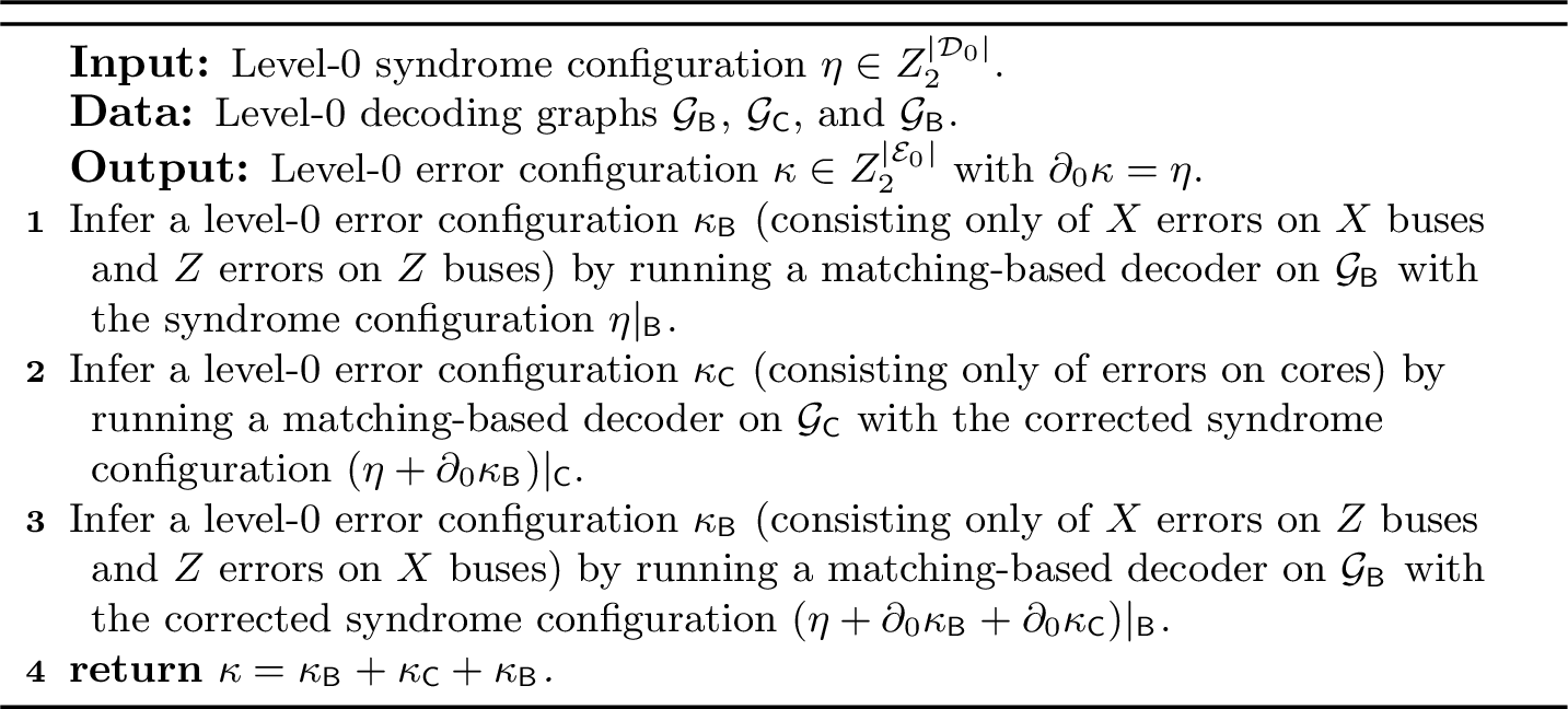
Note that we can combine Algorithm 5 with correlated matching [68] to enhance the decoding performance by taking correlations between \(X\) and \(Z\) errors into account. More specifically, given a level-0 syndrome configuration induced by physical errors, we can first run Algorithm 5, then change the weights of all decoding graphs based on the output following the approach in Ref. [68], and finally run Algorithm 5 again on reweighted decoding graphs. The output of the second run of Algorithm 5 is taken as the level-0 decoding result. We call this procedure above the correlated level-0 decoding. We use the original level-0 decoding routine in Algorithm 5 for theoretical analysis and the correlated level-0 decoding for numerical benchmarking.
Level-1 errorsConsider a collection \(\mathcal{M}\) of readout gadgets, such that the separation between every two \(X\)-basis (or \(Z\)-basis) readout gadgets in \(\mathcal{M}\) is lower bounded by \(\alpha_{\mathsf{c}} d_{0}\) level-0 time steps. We now define level-1 error locations and assign each a corresponding segment. For every core \(\sigma\), readout gadgets in \(\mathcal{M}\) assign a sequence of core-bus CNOT gates \(\Lambda_{t_1},\cdots,\Lambda_{t_{i}}\) (at level-0 time steps \(t_{1}<\cdots<t_{i}\)) and a sequence of bus-core CNOT gates \(\Lambda_{t_{1}'},\cdots,\Lambda_{t'_{j}}\) acting on \(\sigma\) (at level-0 time steps \(t_{1}'<\cdots<t_{j}'\)). Between every two adjacent level-1 CNOT gates with \(\sigma\) on the control side (corresponding to core-bus CNOT gates \(\Lambda_{t_{c}}\) and \(\Lambda_{t_{c+1}}\) with \(c\in\{1,\cdots,i-1\}\)), we assign a level-1 \(X\) error location on the core and define the \(Z\)-basis segment on \(\sigma\) between level-0 time steps \(t_{c}+1\) and \(t_{c+1}\) as the associated segment for the level-1 error location. We assign another two level-1 \(X\) error locations on \(\sigma\), one before the first level-1 CNOT gate corresponding to the core-bus CNOT gate \(\Lambda_{t_1}\) and the other after the last level-1 CNOT gate corresponding to the core-bus CNOT gate \(\Lambda_{t_{i}}\). We define \(Z\)-basis segments on \(\sigma\) before level-0 time step \(t_{1}\) and after level-0 time step \(t_{i}+1\) as the associated segments for the first and the last level-1 \(X\) error locations on \(\sigma\), respectively. See Fig. 6 for an illustration of all level-1 \(X\) error locations set above. Similarly, for the sequence of bus-core CNOT gates, we assign level-1 \(Z\) error locations on the core and define an associated segment for each level-1 \(Z\) error location. For every \(X\) bus \(\sigma'\) of an \(X\)-basis readout gadget in \(\mathcal{M}\), we assign a level-1 \(Z\) error location on \(\sigma'\), which does not propagate out of \(\sigma'\) and only triggers a readout error on the readout gadget. We define the \(X\)-basis segment on \(\sigma'\) spanning over the lifetime of \(\sigma'\) as the associated segment for this level-1 \(Z\) error location. We similarly assign a level-1 \(X\) error location for the \(Z\) bus in every \(Z\)-basis readout gadget in \(\mathcal{M}\) and define the associated bus segment for the level-1 \(X\) error location. These level-1 error locations defined above allow us to perform level-1 decoding. Every level-1 \(X\) (or \(Z\)) error on a level-1 \(X\) (or \(Z\)) error location is called a primitive level-1 error. Every segment associated with a level-1 error location is called a canonical segment.

Every primitive level-1 \(X\) (or \(Z\)) error with an associated canonical segment on a working unit \(\sigma\) between level-0 time steps \(t_1\) and \(t_2\) is equivalent to a logical \(X\) (or \(Z\)) error (as a level-0 error configuration) on \(\sigma\) at the beginning of a level-0 time step \(t\) with \(t_1\leq t\leq t_2\). Let \(\mathsf{E}\) be the collection of all primitive level-1 errors. A level-1 error configuration (as a subset of \(\mathsf{E}\)) is naturally identified with a vector in \(\mathbb{Z}_2^{|\mathsf{E}|}\). Let \(\overline{\partial}_{1}:\mathbb{Z}_2^{|\mathsf{E}|}\to \mathbb{Z}_2^{|\mathcal{D}_1|}\) be the level-1 syndrome map. We construct a level-1 decoding hypergraph \(\mathsf{G}\) with the vertex set \(\mathcal{D}_1\) and the hyperedge set \(\mathsf{E}\), such that each hyperedge \(\mathsf{e}\in\mathsf{E}\) is exactly connected to vertices in \(\overline{\partial}_{1}\mathsf{e}\).
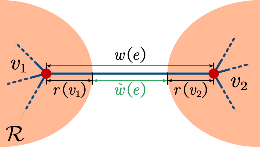
Soft outputs and level-1 error probabilityFor every level-1 error location, we can extract a soft output on the associated canonical segment during the level-0 decoding process to estimate the probability of this level-1 error. This error probability is then converted to the weight of the corresponding hyperedge in the level-1 decoding hypergraph. In the following, we briefly review how to extract the soft output [39] from a segment during a level-0 decoding shot with a sparse-blossom decoder [69]. Consider a non-negatively weighted decoding graph \(\mathcal{G}(w)\) (\(\mathcal{G}\) for short), with \(w\) the assignment of edge weights that maps each edge to a non-negative number. At the end of each decoding shot with a sparse-blossom decoder, a region \(\mathcal{R}\) (combined graph fill region [69]) with an associated radius map \(r\) is constructed on \(\mathcal{G}\), where \(\mathcal{R}\) is a collection of vertices in \(\mathcal{G}\) and \(r\) assigns each vertex in \(\mathcal{G}\) a non-negative radius. Based on the region, we define the postdecoding weight for each edge \(e\in\mathcal{E}\) as \(\tilde{w}(e):=\max(0,w(e)-\sum_{v\in\partial e}r(v))\), where \(\partial e\) denotes the endpoints of \(e\) (Fig. 7). Define a new graph \(\tilde{\mathcal{G}}(\tilde{w})\) with the same vertex and edge structure as \(\mathcal{G}\), and postdecoding weights for all edges.
We are now ready to describe the extraction of the soft output from a segment during a level-0 decoding routine. Consider an \(X\)-basis core segment on the core \(\mathsf{c}\) containing time steps between \(t_1\) and \(t_2\) as shown in Fig. 8.
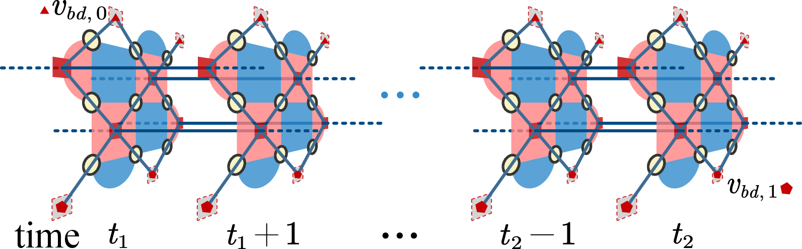
There are two types of boundary edges (weight-1 edges) in the core segment, each corresponding to one of two opposing \(Z\) boundaries. We attach a virtual boundary vertex \(v_{bd,0}\) or \(v_{bd,1}\) to boundary edges corresponding to either boundary. After decoding on \(\mathcal{G}_{\mathsf{C}}\), we obtain a reweighted graph \(\tilde{\mathcal{G}}_{\mathsf{C}}\) by applying the postdecoding reweight procedure described above. The soft output corresponding to the segment is defined as the minimum path length from \(v_{bd,0}\) to \(v_{bd,1}\) on \(\tilde{\mathcal{G}}_{\mathsf{C}}\), and can be efficiently computed by Dijkstra’s algorithm [39]. Soft outputs for other canonical segments are extracted similarly.
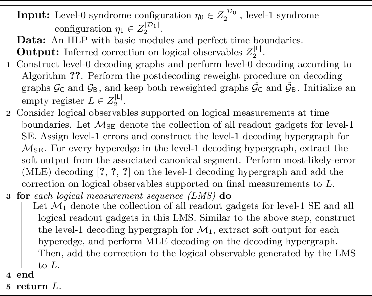
Full decoding procedure Consider an HLP with \(X\)-basis and \(Z\)-basis LMSs under perfect time boundaries. Each LMS generates a logical observable representing the measurement result of the corresponding logical Pauli operator. Moreover, logical measurements at perfect time boundaries may generate additional logical observables. Let \(\mathsf{L}\) be the collection of all logical observables. See Algorithm 9 for the full decoding procedure. Intuitively, we first perform a round of level-0 decoding. Then, at level 1, we decode logical observables supported on logical measurements at time boundaries independently from the other logical observables generated by LMSs. We then decode the logical observable induced by each LMS independently.
2 Induced Level-1 Error Model↩︎
In this section, we theoretically study how physical errors under the phenomenological depolarizing noise model, together with the level-0 decoding result, induce level-1 errors. We first set up the necessary notation for later discussion.
Let \(\mathcal{E}_{\mathrm{dep}}\) be the collection of all primitive level-0 errors in the phenomenological depolarizing noise model. We refer to an element of \(\mathbb{Z}_2^{|\mathcal{E}_{\mathrm{dep}}|}\), which specifies a subset of \(\mathcal{E}_{\mathrm{dep}}\), as a general level-0 error configuration to distinguish it from vectors in \(\mathbb{Z}_2^{|\mathcal{E}_{0}|}\), which are called level-0 error configurations. Since \(\mathcal{E}_{0}\), containing only \(X\) and \(Z\) errors, is a subset of \(\mathcal{E}_{\mathrm{dep}}\), there is a natural injection from \(\mathbb{Z}_{2}^{|\mathcal{E}_{0}|}\) to \(\mathbb{Z}_2^{|\mathcal{E}_{\mathrm{dep}}|}\). Therefore, every level-0 error configuration is also a general level-0 error configuration. We use the same notation \(\partial_{0}\) and \(\partial_{1}\) for the syndrome maps extended from level-0 error configurations to general level-0 error configurations. Define a linear map \(\mathbb{P}_{\mathrm{X}}:\mathbb{Z}_2^{|\mathcal{E}_{\mathrm{dep}}|}\to\mathbb{Z}_2^{|\mathcal{E}_{0}|}\) that maps every primitive level-0 error in \(\mathcal{E}_{\mathrm{dep}}\) to its \(X\)-basis component in \(\mathcal{E}_{0}\). We similarly define \(\mathbb{P}_{\mathrm{Z}}:\mathbb{Z}_2^{|\mathcal{E}_{\mathrm{dep}}|}\to\mathbb{Z}_2^{|\mathcal{E}_{0}|}\). For a general level-0 error configuration \(g\), we define its \(X\)-basis (or \(Z\)-basis) component as \(g_{X}:=\mathbb{P}_{\mathrm{X}}(g)\) (or \(g_Z:=\mathbb{P}_{\mathrm{Z}}(g)\)).
Consider a configuration \(\epsilon\in\mathbb{Z}_2^{|\mathcal{E}_{\mathrm{dep}}|}\) of level-0 physical errors triggering level-0 detectors \(\eta=\partial_{0}\epsilon\). We use Algorithm 5 to obtain an inferred error configuration \(\kappa\in\mathbb{Z}_2^{|\mathcal{E}_{0}|}\) with \(\partial_{0}\kappa=\eta\). Let \(f:=\epsilon+\kappa\), which we call the general residual error configuration. Let \(\mathcal{M}\) be the collection of readout gadgets whose measurement results are of interest. We construct level-1 error locations for \(\mathcal{M}\) and let \(\mathsf{E}\) be the collection of primitive level-1 errors. Let \(\mathcal{D}_{\mathsf{B}_{\blacktriangledown}}\subset\mathcal{D}_{\mathsf{B}_{\blacklozenge}}\) be the subset of detectors in \(\mathcal{D}_{\mathsf{B}_{\blacklozenge}}\) on buses in \(\mathcal{M}\); let \(\mathcal{E}_{\mathsf{B}_{\blacktriangledown}}\) be the subset of errors in \(\mathcal{E}_{\mathsf{B}_{\blacklozenge}}\) on buses in \(\mathcal{M}\). Let \(\partial_{\blacktriangledown}\) be the restricted level-0 syndrome map, which restricts level-0 syndromes to \(\mathcal{D}_{\mathsf{B}_{\lozenge}}\cup \mathcal{D}_{\mathsf{C}}\cup \mathcal{D}_{\mathsf{B}_{\blacktriangledown}}\). We note that level-0 errors in \(\mathcal{E}_{\mathsf{B}_{\blacklozenge}}\backslash\mathcal{E}_{\mathsf{B}_{\blacktriangledown}}\) do not affect readout gadgets in \(\mathcal{M}\). We say two level-0 error configurations \(g_{1}\) and \(g_{2}\) are \(\mathcal{M}\)-equivalentdenoted as \(g_{1}\simeq_{\mathcal{M}}g_{2}\)if they differ by at most a space-time stabilizer (described later) and an error configuration in \(\mathcal{E}_{\mathsf{B}_{\blacklozenge}}\backslash\mathcal{E}_{\mathsf{B}_{\blacktriangledown}}\).
In Sec. 2.1, we prove that \(f\) induces a level-1 error configuration in \(\mathbb{Z}_2^{|\mathsf{E}|}\). This observation guarantees the existence of a solution for our level-1 decoding procedurethe residual error after the level-0 decoding procedure indeed corresponds to a level-1 error configuration. Without loss of generality, we assume \(f\in\mathbb{Z}_2^{|\mathcal{E}_{0}|}\) by decomposing every \(Y\) error in \(\epsilon\) into its \(X\)- and \(Z\)-basis components. We will show that \(f|_{\mathsf{B}_{\lozenge}}\), the residual error restricted to \(\mathcal{E}_{\mathsf{B}_{\lozenge}}\), is equivalent to a level-0 error configuration \(f^{\scriptscriptstyle\square}\) on cores. We say \(f^{\scriptscriptstyle\square}\) is the propagated error from \(f|_{\mathsf{B}_{\lozenge}}\). Then, the combination of the propagated error \(f^{\scriptscriptstyle\square}\) and \(f|_{\mathsf{C}}\) is shown to be \(\mathcal{M}\)-equivalent to the combination of a level-1 error configuration \(\mathsf{f}_{\mathsf{C}}\) on cores and a level-0 error configuration \(f^{\scriptscriptstyle\blacksquare}\) on shuttle buses in \(\mathcal{M}\). Similarly, we say \(f^{\scriptscriptstyle\blacksquare}\) is the propagated errors from \(f^{\scriptscriptstyle\square}+f|_{\mathsf{C}}\), restricted to shuttle buses in \(\mathcal{M}\). We will show that \(f^{\scriptscriptstyle\blacksquare}+f|_{\mathsf{B}_{\blacktriangledown}}\) induces a level-1 error configuration \(\mathsf{f}_{\mathsf{B}}\) on shuttle buses in \(\mathcal{M}\). Finally, we see that \(f\) induces the level-1 error configuration \(\mathsf{f}_{\mathsf{C}}+\mathsf{f}_{\mathsf{B}}\) (or equivalently, \(f\simeq_{\mathcal{M}}\mathsf{f}_{\mathsf{C}}+\mathsf{f}_{\mathsf{B}}\)).
In Sec. 2.2, we show the induced level-1 \(X\) (or \(Z\)) errors almost satisfy a local stochastic noise model.
2.1 Error propagation through hybrid-unit CNOT gates↩︎
We start with a general study of the error propagation phenomena and then analyze \(f\) in detail.
Space-time stabilizers and CNOT membranesA level-0 error configuration that triggers no (level-0 or level-1) detector or logical observable is called a space-time stabilizer [36], [44], [70]. We say two level-0 error configurations \(g_1\) and \(g_2\) are equivalent if they differ by a space-time stabilizer (this is stronger than \(\mathcal{M}\)-equivalence described above). We denote this equivalence relation as \(g_1\simeq g_2\). Thus, we can deform a level-0 error configuration into another equivalent configuration by multiplying the original configuration by space-time stabilizers. For a data qubit \(i\) on a working unit \(\sigma\), denote the collection of \(X\) (or \(Z\)) stabilizer generators of the working unit supported on qubit \(i\) as \(\delta_{X,i}\) (or \(\delta_{Z,i}\)). At a level-0 time step \(t\), let \(\Lambda_{t}\) denote the depth-1 layer of hybrid CNOT gates; let \(e_{A,i,t}\) denote the \(A\)-basis (\(A\in\{X,Z\}\)) data qubit error on qubit \(i\); let \(e_{\mathrm{S},t}\) denote the measurement error on stabilizer \(\mathrm{S}\). If qubit \(i\) is not acted on by \(\Lambda_{t}\), then \(X\) errors \(e_{X,i,t}\), \(e_{X,i,t+1}\) on this qubit at the level-0 time steps \(t\) and \(t+1\), together with stabilizer measurement errors \(\{e_{\mathrm{S},t}|\mathrm{S}\in\delta_{Z,i}\}\) at level-0 time step \(t\), form a spacetime stabilizer. Similarly, \(e_{Z,i,t}+e_{Z,i,t+1}+\sum_{\mathrm{S}\in \delta_{X,i}}e_{\mathrm{S},t}\) is also a spacetime stabilizer. Now consider the case where qubit \(i\) is acted on by \(\Lambda_{t}\). Denote the qubit that participated in the same physical CNOT gate as \(i\) in \(\Lambda_{t}\) as \(j\). If qubit \(i\) is on the target side of \(\Lambda_t\), then \(e_{Z,i,t}+e_{Z,i,t+1}+e_{Z,j,t}+\sum_{\mathrm{S}\in\delta_{X,i}}e_{\mathrm{S},t}\) is a spacetime stabilizer. Notice that the level-0 error configuration \(e_{Z,i,t}+e_{Z,i,t+1}+\sum_{\mathrm{S}\in\delta_{X,i}}e_{\mathrm{S},t}\) on the working unit \(\sigma\) is now equivalent to the qubit error \(e_{Z,j,t}\) on a different working unit. This gives rise to the error propagation phenomenon that we mentioned at the beginning of Sec. 2. We define a CNOT membrane associated with \(\Lambda_{t}\) for the \(X\)-basis decoding subgraph on the working unit \(\sigma\) as a plane with a time coordinate \(t+\frac{1}{2}\) (only in the coordinate system of the subgraph). We say every \(X\) stabilizer measurement error on \(\sigma\) at level-0 time step \(t\) is on the CNOT membrane. Moreover, we say a level-0 error configuration intersects with this CNOT membrane if the configuration contains at least one primitive level-0 error on the CNOT membrane. See Fig. 10 for an illustration of space-time stabilizers and a CNOT membrane.
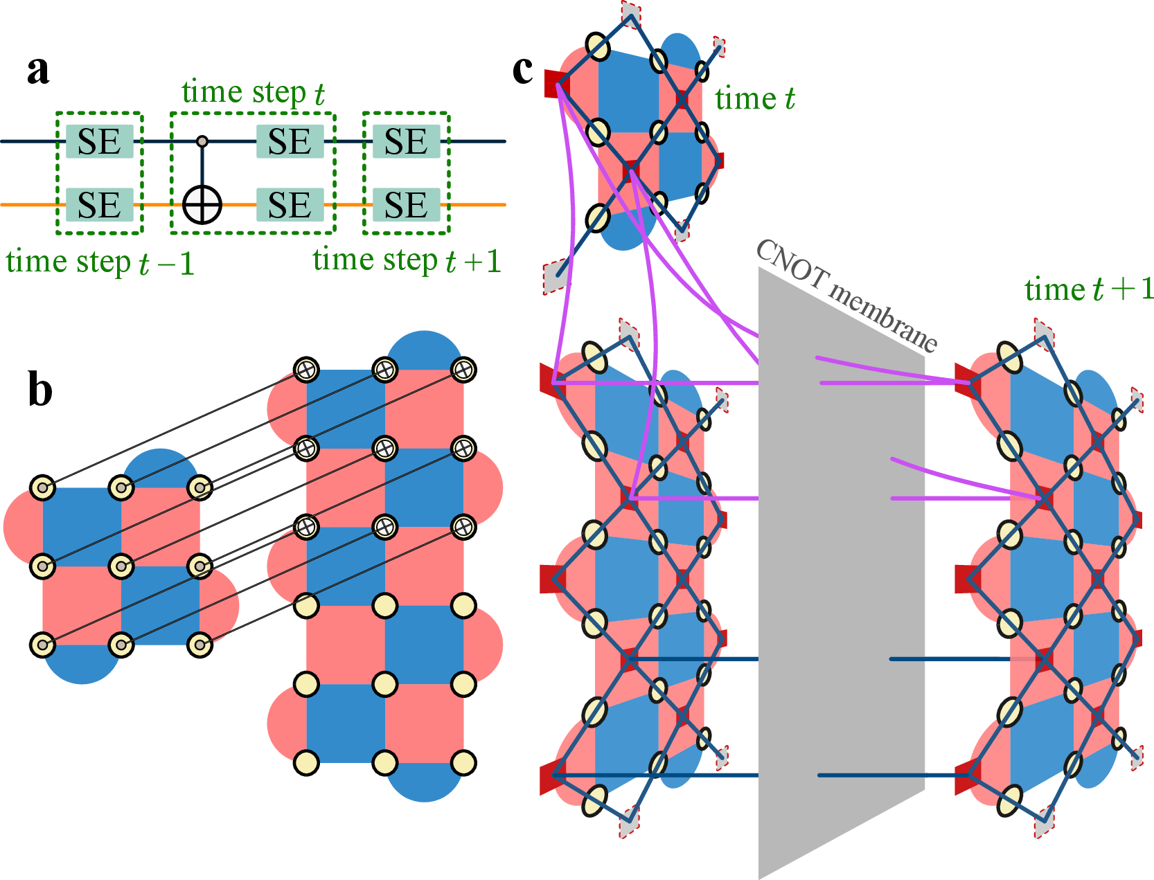
Similarly, if qubit \(i\) is on the control side, then \(e_{X,i,t}+e_{X,i,t+1}+e_{X,j,t}+\sum_{\mathrm{S}\in\delta_{Z,i}}e_{\mathrm{S},t}\) is a spacetime stabilizer. In this case, we define a CNOT membrane associated with \(\Lambda_t\) on \(\sigma\) as a plane with a time coordinate \(t+\frac{1}{2}\) in the coordinate system of the \(Z\)-basis decoding subgraph for \(\sigma\).
Walks, paths, and cyclesBorrowing from standard terminologies of walks, paths, and cycles on a graph in graph theory [71], we define these terms as sequences of primitive level-0 errors on a decoding subgraph in the following. Consider an \(X\)- or \(Z\)-basis decoding subgraph for a working unit \(\sigma\). We introduce an additional virtual vertex \(v_{\varnothing}\) (representing the lack of a vertex), which is considered an endpoint for every boundary edge in the decoding subgraph. A walk \(\omega\) on the decoding subgraph is a sequence of primitive level-0 errors \(e_1,\cdots,e_{r}\) (each corresponds to an edge in the decoding subgraph), such that there is a sequence of vertices \(v_{0},\cdots,v_{r}\) on the decoding graph satisfying the following conditions: (i) only vertices \(v_{0}\) and \(v_{r}\) are allowed to be \(v_{\varnothing}\) (in other words, only \(e_{1}\) and \(e_{r}\) are allowed to be boundary edges), and (ii) for every \(i\in\{1,\cdots,r\}\), both \(v_{i-1}\) and \(v_{i}\) are endpoints of \(e_{i}\). The vertex sequence \(v_{0},\cdots,v_{r}\) is referred to as the vertex trail of \(\omega\). A subwalk of \(\omega\) is a subsequence of \(\omega\). Each walk \(\omega\) is associated with a level-0 error configuration, \([\omega]\), as the sum of all primitive level-0 errors in \(\omega\) as vectors over \(\mathbb{Z}_2\). This level-0 error configuration \([\omega]\) is called the error value of \(\omega\). If \(\omega\) contains no repeated primitive level-0 errors, then we can safely identify \(\omega\) with \([\omega]\). We let \(|\omega|\) denote the length of the sequence \(\omega\) and \(|[\omega]|\) denote the weight of \([\omega]\). Similarly, consider a collection of walks \(\overline{\omega}\), we define its error value \([\overline{\omega}]\) as the sum of all primitive level-0 errors in \(\overline{\omega}\) as vectors over \(\mathbb{Z}_2\). We also identify \(\overline{\omega}\) with \([\overline{\omega}]\) if \(\overline{\omega}\) contains no repeated level-0 primitive errors; we let \(|\overline{\omega}|\) denote the sum of lengths of all walks in \(\overline{\omega}\) and \(|[\overline{\omega}]|\) denote the weight of \([\overline{\omega}]\). We introduce two subscripts \(||\) and \(\perp\), representing the qubit-error component and the stabilizer-measurement-error component, respectively. In this way, \(|\overline{\omega}_{||}|\) and \(|\overline{\omega}_{\perp}|\) denote the number of occurrences of qubit errors and stabilizer measurement errors in \(\overline{\omega}\) (rather than in its error value \([\overline{\omega}]\)), respectively. Similarly, this definition also applies to individual walks and error configurations. We say a walk \(\omega\) is closed if the starting vertex coincides with the ending vertex in the vertex trail of \(\omega\). A simple walk is a walk with no repeated primitive level-0 errors. A walk \(\omega\) with its vertex trail \(v_{0},\cdots,v_{r}\) is a path if all these vertices are disjoint; the walk \(\omega\) is a cycle if the only repeated vertices in the vertex trail are \(v_{0}\) and \(v_{r}\). A closed walk can be decomposed as a collection of cycles; a walk that is not closed can be decomposed as a path and a collection of cycles. We note that every walk that we analyze in the following has no repeated primitive level-0 errors on any CNOT membrane.
Classification of closed walks on decoding graphsWe classify closed walks in an \(X\)-basis or \(Z\)-basis decoding subgraph on a working unit into the following categories.
Lightning walk. A lightning walk is a closed walk terminating at two opposite spatial boundaries. A canonical lightning walk is a lightning walk that does not intersect with any CNOT membrane.
Sprout walk. A sprout walk is a closed walk terminating at a time boundary. A benign sprout walk is a sprout walk that does not intersect with any CNOT membrane. A benign sprout walk does not propagate errors.
Cross-membrane walk. A cross-membrane walk is a closed walk that does not belong to the above two categories and intersects with at least one CNOT membrane.
Benign walk. A benign walk is a closed walk that does not belong to the above three categories. The error value of a benign walk is a level-0 space-time stabilizer.
We establish the following two lemmas. The first allows us to equivalently deform a lightning walk into a canonical lightning walk and a collection of benign and cross-membrane walks. The second shows that the error value of a sprout walk is equivalent to the combination of benign sprout cycles and cross-membrane cycles.
Lemma 1. If a lightning walk \(\ell\) on a working unit \(\sigma\) intersects with at least one CNOT membrane and has no repeated edges on it, we can find a sequence \(g\) of error paths on \(\sigma\) such that (i) \(g\) also forms a canonical lightning walk, (ii) each path in \(g\) is immediately after the earliest CNOT membrane intersected by \(\ell\), and (iii) we can rearrange edges in \(\ell\) and paths in \(g\) into a collection of cross-membrane walks and benign walks. We regard \(g\) also as a canonical lightning walk and refer to it as the canonical retraction of \(\ell\).
Proof. Denote the earliest CNOT membrane intersected by \(\ell\) as \(\mathfrak{m}\). As \(\ell\) terminates at two opposing space boundaries, we introduce two virtual boundary vertices \(v_{bd,0}\) and \(v_{bd,1}\) for these two space boundaries, respectively. We connect each virtual boundary vertex to the boundary edges terminating on the corresponding space boundary. Without loss of generality, we suppose \(\ell\) starts with a boundary edge connected to \(v_{bd,0}\) and ends with a boundary edge connected to \(v_{bd,1}\). By traversing \(\ell\), we obtain an ordered sequence of time-like edges \(e_1, e_2, \cdots, e_r\) on \(\mathfrak{m}\), corresponding to stabilizer measurement errors. For each edge \(e_i\), denote its endpoints before and after \(\mathfrak{m}\) on \(\sigma\) as \(\partial_{<}e_i\) and \(\partial_{>}e_i\), respectively. Let \(l_i\) (\(0<i<r\)) be the subwalk in \(\ell\) between \(e_{i}\) and \(e_{i+1}\) (excluding both \(e_{i}\) and \(e_{i+1}\)); let \(l_{0}\) be the subwalk in \(\ell\) from \(v_{bd,0}\) to \(e_1\) (excluding \(e_{1}\)); let \(l_{r}\) be the subwalk in \(\ell\) from \(e_{r}\) to \(v_{bd,1}\) (excluding \(e_{r}\)). In this way, \(\ell\) is exactly the sequence \((l_0,e_{1},l_1,e_2,l_2,\cdots,e_r,l_r)\). Moreover, subwalks \(l_0,\cdots,l_r\) alternate between the two sides of \(\mathfrak{m}\). We introduce \(g_0\) (or \(g_r\)) as the minimum-weight path connecting the vertex \(\partial_{>}e_1\) (or \(\partial_{>}e_{r}\)) to the spatial boundary resided by \(v_{bd,0}\) (or \(v_{bd,1}\)). For \(i\in\{1,2,\cdots,r-1\}\), we introduce \(g_{i}\) as the minimum-weight path connecting \(\partial_{>}e_{i}\) and \(\partial_{>}e_{i+1}\). Define the sequence \(g:=(g_{0},\cdots,g_{r})\), which is immediately after \(\mathfrak{m}\) by construction. Then, the sequence \(g\) also forms a canonical lighting walk.
We now show that we can rearrange subwalks in the sequence representing \(\ell\) \[\label{eq:32subwalk32sequence} (l_0,e_1,l_1,\cdots,e_r,l_r)\tag{1}\] and paths in \(g=(g_{0},\cdots,g_{r})\) into a collection of cross-membrane walks and benign walks. For every subwalk \(l_a\) before \(\mathfrak{m}\), we can pair it with its neighboring on-membrane edge(s) and a corresponding path in \(g\) to form a cross-membrane walk; for every subwalk \(l_b\) after \(\mathfrak{m}\), we can pair it with a corresponding path in \(g\) to form a benign walk. We describe the detailed construction as follows. If \(l_0\) lies before \(\mathfrak{m}\), we can see that \((l_0,e_{1},g_{0})\) forms a cross-membrane walk. Then in this case, for any non-negative even (or odd) integer \(a\leq r\), \(l_{a}\) is before (or after) \(\mathfrak{m}\). Thus, for a non-negative odd index \(a\leq r\), \((l_a,g_a)\) forms a benign walk; for a positive even index \(a<r\), \((e_{a},l_a,e_{a+1},g_{a})\) forms a cross-membrane walk. Finally, if \(r\) is even, then \((l_r,e_r,g_r)\) forms a cross-membrane walk. In this way, we rearrange subwalks in \(\ell\) and paths in \((g_{0},\cdots,g_{r})\) into the collection of cross-membrane walks and benign walks above. We note that each subwalk of the sequence in Eq. 1 and each path in \(g\) is contained exactly once in these walks. A similar argument also holds if \(l_0\) is after \(\mathfrak{m}\). Therefore, we have successfully obtained \(g\) that satisfies all three conditions in the lemma. See Fig. 11 for two examples illustrating the above procedure. ◻
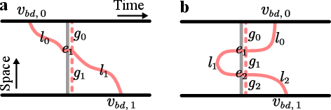
Lemma 2. For a sprout walk \(\ell\) that intersects with at least one CNOT membrane, we can find a level-0 error configuration \(g\) on the same working unit as \(\ell\), such that (i) \(g\) is the combination of benign sprout cycles and (ii) \(g+[\ell]\) is equivalent to a collection of cross-membrane cycles.
Proof. Denote the two boundary edges of \(\ell\) as \(e_1\) (a time-boundary edge) and \(e_{-1}\), respectively. If \(\ell\) only terminates at time boundaries, then define \(g_1\) as the minimum-weight error path connecting the (non-virtual) endpoint of \(e_1\) to a space boundary, and \(g_{-1}\) as the minimum-weight path connecting the endpoint of \(e_{-1}\) to the same space boundary. Define a level-0 error configuration \(g:=(g_1+e_1)+(g_{-1}+e_{-1})\), which is composed of two benign sprout cycles \((g_{1}+e_{1})\) and \((g_{-1}+e_{-1})\). We can see that \(g+[\ell]\) does not terminate at time boundaries and should be equivalent to a combination of cross-membrane cycles. On the other hand, if \(\ell\) also terminates at a space boundary, then \(e_{-1}\) is a space-boundary edge. Define a level-0 error configuration \(g_1\) as the minimum-weight path connecting the vertex of \(e_{1}\) to the same space boundary as \(e_{-1}\). Then, we can find a benign sprout cycle \(g:=g_1+e_1\) satisfying the requirements in the lemma. ◻
Error propagationIn the following, we show (i) how canonical \(X\)-basis (or \(Z\)-basis) lightning cycles on an \(X\) (or \(Z\)) bus propagate errors to cores through CNOT membranes, and (ii) how cross-membrane walks propagate errors through CNOT membranes. The latter is a recurrently used technique in Sec. 2.2.

Lemma 3. Consider a \(Z\)-basis (or \(X\)-basis) canonical lighting cycle \(\ell\) on a \(Z\) (or \(X\)) bus \(\sigma\). Suppose CNOT membranes on this bus after \(\ell\) correspond to hybrid-unit CNOT gates \(\Lambda_{t_1},\cdots,\Lambda_{t_{o}}\) at level-0 time steps \(t_{1}<\cdots<t_{o}\), respectively. Then, the lightning cycle \(\ell\) propagates to canonical lightning cycles at level-0 time step \(t_i\) on every core on the control side (or target side) of the core-bus (or bus-core) CNOT gate \(\Lambda_{t_i}\) for all \(i\in\{1,\cdots,o\}\).
Proof. Without loss of generality, we assume \(\sigma\) is a \(Z\) bus. Let \(\ell_\sigma\) be the logical operator along a long edge of \(\sigma\); let \(\ell_{\sigma,t}\) be the level-0 error configuration corresponding to \(\ell_{\sigma}\) at level-0 time step \(t\). Then, the cycle \(\ell\) is equivalent to the level-0 error configuration \(\ell_{\sigma,t_1}\). We can see that \(\ell_{\sigma,t_1}\) is equivalent to \(\left(\Lambda_{t_1}(\ell_{\sigma,t_1})+\ell_{\sigma,t_1}\right)+\ell_{\sigma,t_1+1}\), where the first term is the product of logical \(Z\) operators on every core at the control side of \(\Lambda_{t_1}\) at level-0 time step \(t_1\) and the second term (at level-0 time step \(t_1+1\)) is equivalent to \(\ell_{\sigma,t_2}\). The lemma is proven by recursively applying the argument above. ◻
Lemma 4 (Error propagation of a cross-membrane walk). Consider a cross-membrane walk \(\ell\) on a working unit \(\sigma\) that intersects the CNOT membranes associated with hybrid-unit CNOT gates \(\Lambda_{t_1},\cdots,\Lambda_{t_o}\) at level-0 time steps \(t_{1}<\cdots<t_{o}\), respectively. Then, the level-0 error configuration \([\ell]\) is equivalent to a level-0 error configuration \(u:=u_{t_1}+\cdots+u_{t_o}\), where each \(u_{t_i}\) (\(i\in\{1,\cdots,o\}\)) as a level-0 error configuration is a collection of simple walks at level-0 time step \(t_{i}\) on working units on the opposite side of \(\Lambda_{t_i}\) to \(\sigma\). (We also say \(\ell\) propagates to \(u\).) Moreover, for each \(u_{t_i}\), (i) every simple walk in \(u_{t_i}\) either terminates at a spatial boundary or at the pointy end of an error in \(\ell\) on the CNOT membrane at \(t_i+\frac{1}{2}\), and (ii) its weight, \(|u_{t_i}|\), is upper bounded by \(|\ell_{||}|/2\), with \(|\ell_{||}|\) the number of occurrences of qubit errors in \(\ell\).
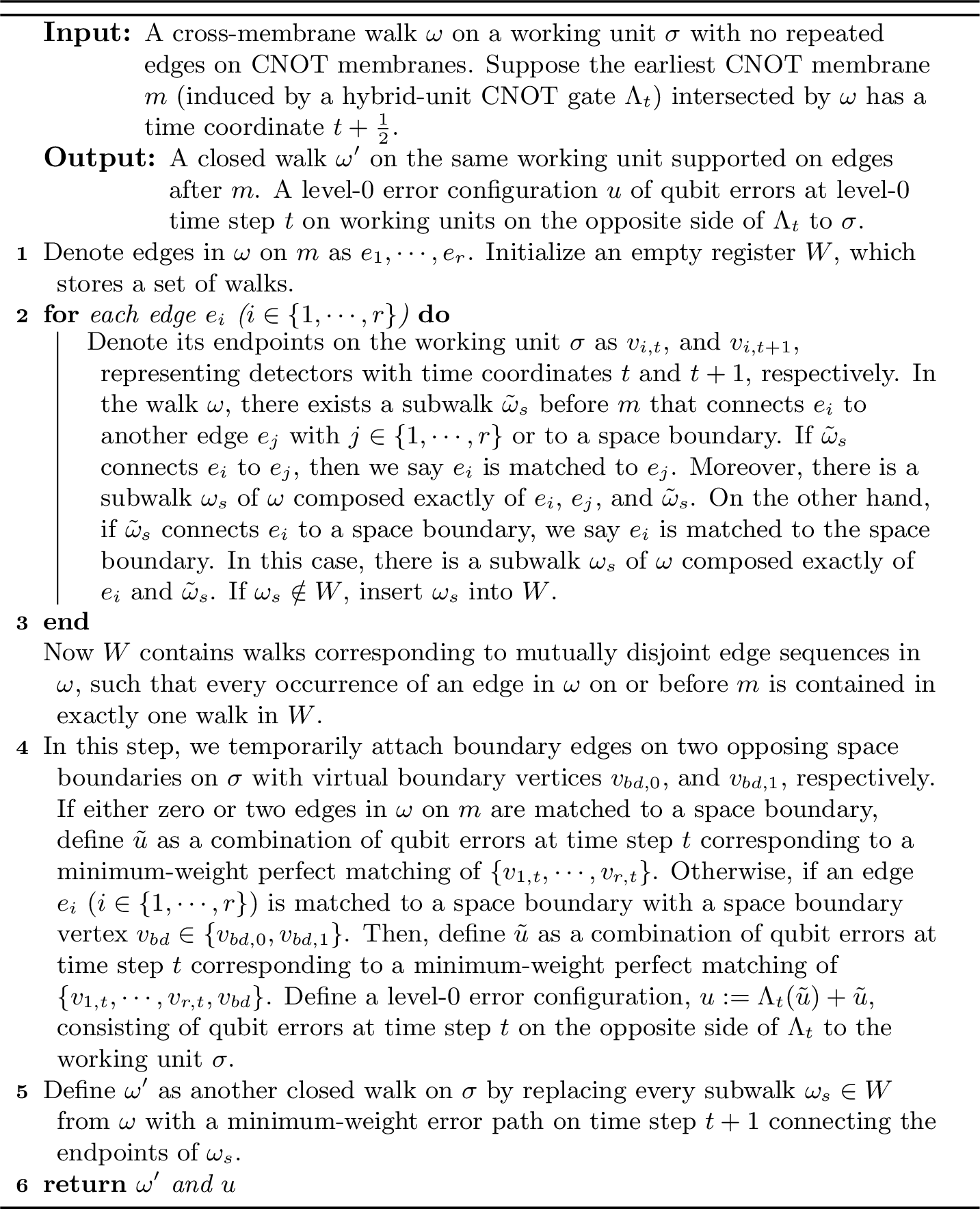
Proof. The proof proceeds by recursively deforming \(\ell\) across the earliest CNOT membrane intersected by it and recording the corresponding propagated error. The deformation is implemented by multiplying \(\ell\) with space-time stabilizers. More specifically, in Algorithm 13, we show how to obtain a closed walk \(\ell_1\) and a level-0 error configuration \(u_{t_1}\) with \([\ell]\simeq [\ell_1]+u_{t_1}\) such that (i) the closed walk \(\ell_1\) lies after the CNOT membrane at \(t_{1}+\frac{1}{2}\) and only intersects with \(o-1\) CNOT membranes (corresponding to hybrid-unit CNOT gates \(\Lambda_{t_2},\cdots,\Lambda_{t_{o}}\)), and (ii) the error configuration \(u_{t_1}\) consists of qubit-error simple walks on the opposite side of \(\Lambda_{t_1}\) and satisfies condition (i) in the lemma. Denote the weight of qubit errors in \([\ell]\) before (or after) the CNOT membrane \(\mathfrak{m}\) as \(|[\ell]_{||,<}|\) (or \(|[\ell]_{||,>}|\)). According to the minimum-weight constraint in the third step of Algorithm 13, we can see that \(|u_{t_1}|\leq |[\ell]_{||,<}|\) and \(|u_{t_1}|\leq|[\ell]_{||,>}|\). Thus, the weight of \(u_{t_1}\) is upper bounded by \(\max(|[\ell]_{||,<}|,|[\ell]_{||,>}|)\leq|[\ell]_{||}|/2\leq |\ell_{||}|/2\). See Fig. 12 for an example illustrating the procedure in Algorithm 13.
We can then apply Algorithm 13 again on \(\ell_1\) to obtain another closed walk \(\ell_2\) (intersecting with \(o-2\) CNOT membranes) and a level-0 error configuration \(u_{t_2}\) with \([\ell_1]\simeq [\ell_{2}]+u_{t_2}\). Thus, by recursively applying Algorithm 13, we can obtain a series of closed walks \(\ell_{1},\cdots,\ell_{o}\) and a series of level-0 error configurations \(u_{t_1},\cdots,u_{t_{o}}\), such that (i) \(\ell_{i}\) intersects with \(o-i\) CNOT membranes corresponding to hybrid-unit CNOT gates \(\Lambda_{t_{i+1}},\cdots,\Lambda_{t_{o}}\) for every \(i\in\{1,\cdots,o-1\}\), (ii) \([\ell_{o}]\) is a space-time stabilizer, (iii) every \(u_{t_i}\) satisfies the first requirement in the lemma, and (iv) \([\ell_{i}]\simeq[\ell_{i+1}]+u_{t_{i+1}}\) for every \(i\in\{1,\cdots,o-1\}\). Thus, we can see that \([\ell]\simeq [\ell_{1}]+u_{t_1}\simeq\cdots\simeq u_{t_1}+\cdots+u_{t_{o}}\). Notice that each \(u_{t_i}\) can also be obtained by erasing all CNOT membranes before the \(i\)th CNOT membrane and then running the Algorithm 13 on \(\ell\). Thus, the weight of \(u_{t_i}\) is also upper bounded by \(|\ell_{||}|/2\). ◻
We now return to the analysis of the level-0 residual error configuration \(f\in\mathbb{Z}_2^{|\mathcal{E}_{0}|}\) introduced at the beginning of this section.
Lemma 5. The level-0 residual error configuration \(f\) is \(\mathcal{M}\)-equivalent to a level-1 error configuration.
Proof. On a high level, this proof successively cleans closed walks in \(\mathcal{E}_{\mathsf{B}_\lozenge}\), cores, and finally in \(\mathcal{E}_{\mathsf{B}_{\blacktriangledown}}\). At each stage, closed walks either propagate to the next stage or are absorbed as level-1 errors. As \((\partial_{0}f|_{\mathsf{B}_{\lozenge}})|_{\mathsf{B}_{\lozenge}}=(\partial_{0}f)|_{\mathsf{B}_\lozenge}=0\), \(f|_{\mathsf{B}_{\lozenge}}\) is a collection of cycles, each of which is either an \(X\)-basis cycle on an \(X\) bus or a \(Z\)-basis cycle on a \(Z\) bus. According to Lemma 1 and Lemma 2, \(f|_{\mathsf{B}_{\lozenge}}\) can be equivalently deformed into a collection of benign sprout cycles, benign cycles, canonical lightning cycles, and cross-membrane cycles. The first two types of cycles are equivalent to no error. The last two types of cycles are equivalent to a level-0 error configuration \(f^{\scriptscriptstyle \square}\) on cores according to Lemma 3 and Lemma 4. Thus, we see that \(f|_{\mathsf{B}_{\lozenge}}\simeq f^{\scriptscriptstyle\square}\). Similarly, as \((\partial_{0}f^{\scriptscriptstyle\square}+\partial_{0}f|_{\mathsf{C}})|_{\mathsf{C}}=(\partial_{0}f|_{\mathsf{B}_{\lozenge}}+\partial_{0}f|_{\mathsf{C}})|_{\mathsf{C}}=(\partial_0f)|_{\mathsf{C}}=0\), we can see that \(f^{\scriptscriptstyle\square}+f|_{\mathsf{C}}\) is equivalent to a collection of canonical lightning cycles and cross-membrane cycles on cores. Each canonical lightning cycle on a core is equivalent to the level-1 primitive core error, whose associated canonical segment contains this lightning cycle. Let \(\mathsf{f}_{\mathsf{C}}\) be the level-1 error configuration on cores induced by the canonical lightning cycles in \(f^{\scriptscriptstyle\square}+f|_{\mathsf{C}}\). The cross-membrane cycles on cores introduced by \(f^{\scriptscriptstyle\square}+f|_{\mathsf{C}}\) propagate to a level-0 error configuration \(f^{\scriptscriptstyle\blacksquare}\) of \(Z\) errors on \(X\) buses and \(X\) errors on \(Z\) buses in \(\mathcal{M}\) according to Lemma 4. Finally, as \((\partial_{0}f^{\scriptscriptstyle\blacksquare}+\partial_{0}f|_{\mathsf{B}_{\blacktriangledown}})|_{\mathsf{B}_{\blacktriangledown}}=(\partial_{0}f)|_{\mathsf{B}_{\blacktriangledown}}=0\), the error configuration \(f^{\scriptscriptstyle\blacksquare}+f|_{\mathsf{B}_{\blacktriangledown}}\) is equivalent to a collection of canonical lightning cycles on shuttle buses in \(\mathcal{M}\), which incurs a level-1 error configuration \(\mathsf{f}_{\mathsf{B}}\) on them. Thus, according to the following equation, \(f\) is \(\mathcal{M}\)-equivalent to the level-1 error configuration \(\mathsf{f}_{\mathsf{C}}+\mathsf{f}_{\mathsf{B}}\). \[\begin{align} \large f=&f|_{\mathsf{B}_{\lozenge}} + f|_{\mathsf{C}} + f|_{\mathsf{B}_{\blacklozenge}} \simeq f^{\scriptscriptstyle\square} + f|_{\mathsf{C}}+f|_{\mathsf{B}_{\blacklozenge}}\nonumber\\ \simeq&_{\mathcal{M}}\;\mathsf{f}_{\mathsf{C}} + f^{\scriptscriptstyle\blacksquare}+f|_{\mathsf{B}_{\blacktriangledown}} \simeq \mathsf{f}_{\mathsf{C}}+\mathsf{f}_{\mathsf{B}} \end{align}\] ◻
2.2 Error Reduction Theorem↩︎
Throughout this subsection, we fix the compilation parameter \(\alpha_{\mathsf{b}}=d_{1}\) and ensure that every pair of \(X\)-basis or \(Z\)-basis readout gadgets in \(\mathcal{M}\) is separated by at least \(d_{0}\) level-0 time steps. In this case, we will show that the probability distribution of induced level-1 \(X\) (or \(Z\)) errors satisfies a local stochastic noise model except for a rare event whose probability is exponentially suppressed in \(d_{0}d_1\).
Without loss of generality, we consider level-1 \(X\) errors. For now, we assume that \(f\) consists only of level-0 \(X\) errors. We now perform a more fine-grained analysis on \(f\). According to the proof of Lemma 5, we know that there are two types of errors on cores: one is the propagated errors (each is a simple walk according to Lemma 4) from \(X\)-basis closed walks on \(X\) buses; the other is the native errors in \(f|_{\mathsf{C}}\). Similarly, there are two types of \(X\)-basis errors on \(Z\) buses: one propagated from cores and the other in \(f|_{\mathsf{B}_{\blacktriangledown}}\). We often need to consider propagated errors and native errors in \(f\) as distinct objects to track their respective weights. In this section, we regard \(f\) as a set of length-1 walks, referred to as native walks, each of which corresponds to a unique primitive level-0 error in \(f\). Then, every level-0 error configuration contained in \(f\) is regarded as a subset of \(f\). Propagated simple walks are treated as distinct objects and are not identified with native walks, even when they have overlapping supports.
We know that \(f|_{\mathsf{B}_{\lozenge}}\) is a collection of error cycles \(\{\tilde{\ell}_{1},\cdots,\tilde{\ell}_{r}\}\) on \(X\) buses. We restrict to the case where each cycle in \(f|_{\mathsf{B}_{\lozenge}}\) has a weight smaller than \(d_{0}d_{1}\). (The probability for a cycle of weight at least \(d_0d_1\) is so heavily suppressed that we can regard such an event as failure without analyzing it.) In this case, every cycle in \(f|_{\mathsf{B}_{\lozenge}}\) is either a benign sprout cycle, a benign cycle, or a cross-membrane cycle that only intersects with a single CNOT membrane. For each \(\tilde{\ell}_{i}\) (\(i\in\{1,\cdots,r\}\)), let \(\tilde{\ell}_{i}^{\circ}\) be a set of propagated simple walks, representing the propagated errors from \(\tilde{\ell}_i\). If \(\tilde{\ell}_i\) is a benign cycle or a benign sprout cycle, then \(\tilde{\ell}_i^{\circ}\) is an empty set. Otherwise, we obtain \(\tilde{\ell}_{i}^{\circ}\) as a set of propagated simple walks on cores, following Lemma 4. We say \(\tilde{\ell}_i\) is the source for every propagated simple walk in \(\tilde{\ell}_{i}^{\circ}\). Define \(f^{\circ}:=\bigcup \tilde{\ell}_i^{\circ}\), the collection of propagated simple walks on cores from \(\{\tilde{\ell}_1,\cdots,\tilde{\ell}_r\}\). We note that \(f^{\circ}\) may contain repeated level-0 primitive errors; thus, we need to differentiate the set from its error value \([f^{\circ}]\). Moreover, as \(\tilde{\ell}_i\simeq \tilde{\ell}_i^{\circ}\), we know that the error configuration \([f^{\circ}]\) is equivalent to \(f|_{\mathsf{B}_{\lozenge}}\). The propagated simple walks in \(f^{\circ}\), together with the native walks in \(f|_{\mathsf{C}}\), can be partitioned into a set of closed walks \(\{\ell_{1},\cdots,\ell_{o}\}\) on cores, such that (i) each closed walk \(\ell_{j}\) is composed of propagated simple walks in \(f^{\circ}\) and native walks in \(f|_{\mathsf{C}}\) and (ii) every simple walk in \(f^{\circ}\), as well as every native walk in \(f|_{\mathsf{C}}\), is contained in exactly one closed walk in \(\{\ell_{1},\cdots,\ell_{o}\}\). We also view each closed walk \(\ell_{j}\) as a set of the constituent propagated simple walks in \(f^{\circ}\) and native walks in \(f|_{\mathsf{C}}\). In this way, the disjoint union of two sets of walks \(f^{\circ}\cup f|_{\mathsf{C}}\) is also the disjoint union of \(\ell_{1},\cdots,\ell_{o}\).
For each \(\ell_j\), we will define its propagation \(\ell_j^{\bullet}\) as a set of simple walks on \(Z\) buses in \(\mathcal{M}\); and we also say \(\ell_j\) is the source for every simple walk in \(\ell_j^{\bullet}\). If \(\ell_j\) is a benign walk, then \(\ell_j^{\bullet}\) is an empty set. If \(\ell_j\) is a cross-membrane walk, define \(\ell_j^{\bullet}\) as the set of simple walks propagated from \(\ell_j\) according to Lemma 4. If \(\ell_i\) is a lightning walk, according to Lemma 1, we can find the canonical retraction \(g_j\) of \(\ell_j\), such that we can arrange \(\ell\) and paths in \(g_{i}\) into a collection of cross-membrane walks and benign walks. Define \(\ell_j^{\bullet}\) as the set of all simple walks propagated from these cross-membrane walks. Define \(f^{\bullet}:=\bigcup \ell_j^{\bullet}\) as the set of all simple walks on buses in \(\mathcal{M}\) propagated from \(\{\ell_1,\cdots,\ell_o\}\). Similarly, the set of walks \(f^{\bullet}\cup f|_{\mathsf{B}_{\blacktriangledown}}\) can be decomposed as a disjoint union of closed walks on \(Z\) buses. We refer to each such closed walk as a closed walk in \(f^{\bullet}\cup f|_{\mathsf{B}_{\blacktriangledown}}\). We say a closed walk in \(f^{\bullet}\cup f|_{\mathsf{B}_{\blacktriangledown}}\) is native if the closed walk only consists of native walks in \(f|_{\mathsf{B}_{\blacktriangledown}}\). We say two closed walks \(\ell_{a}\) and \(\ell_{b}\) on cores are linked if a simple walk in \(\ell_a^{\bullet}\) and a simple walk in \(\ell_{b}^{\bullet}\) belong to the same closed walk in \(f^{\bullet}\cup f|_{\mathsf{B}_{\blacktriangledown}}\) on a \(Z\) bus. We can then construct a graph \(\mathcal{W}_{\mathsf{C}}\) with closed walks in \(\{\ell_{1},\cdots,\ell_o\}\) as vertices, such that two vertices are connected by an edge if and only if the corresponding closed walks are linked.
Definition 3 (Downstream web). Consider a collection \(w\) of \(X\)-basis walks on cores and native walks on \(Z\) buses, such that (i) the subcollection of walks on cores, \(w|_\mathsf{C}\), is the union of a subcollection of closed walks (each as a set of walks) in \(\{\ell_1,\cdots,\ell_{o}\}\), (ii) the subcollection of native walks on \(Z\) buses, \(w|_{\mathsf{B}_{\blacktriangledown}}\subset f|_{\mathsf{B}_{\blacktriangledown}}\) contains no native closed walks, and (iii) \(\partial_{\blacktriangledown}[w]=0\). We say \(w\) is a downstream web if \(w|_{\mathsf{C}}\) corresponds to a connected component in the graph \(\mathcal{W}_{\mathsf{C}}\). We say a closed walk \(\ell_{i}\in\{\ell_{1},\cdots,\ell_{o}\}\) is in \(w\) if \(\ell_i\) is a subset of \(w\). Moreover, we say a downstream web \(w\) is a native downstream web if every closed walk in \(w|_{\mathsf{C}}\) contains no simple walks in \(f^{\circ}\). (Notice that every native downstream web \(w\) is composed of native walks and is contained in \(f\).)
In this way, we can see that \(f^{\circ}\cup( f|_{\mathsf{C}}\cup f|_{\mathsf{B}_{\blacktriangledown}})\) is a disjoint union of downstream webs and native closed walks on \(Z\) buses.
We now set bounds on native downstream webs and then set bounds on \(f\). We start with two definitions. First, we define a level-0 adjacency graph \(\mathcal{A}\) [7], whose vertices are identified with level-0 error locations, such that every two vertices are connected by an edge if and only if their corresponding primitive level-0 errors overlap in their level-0 syndromes. This construction [7] is a standard technique in fault-tolerance proofs to help with combinatorial analysis of errors. Secondly, we define sets of primitive level-0 \(X\) errors in \(\mathcal{E}_{0}\) that may contribute to primitive level-1 \(X\) errors on cores and \(Z\) buses, respectively.
Definition 4 (Receptive zone for a primitive level-1 error). Consider a primitive level-1 \(X\) error \(\mathsf{e}\) associated with a canonical segment \(\mathrm{G}\) on a working unit \(\sigma\). The receptive zone for \(\mathsf{e}\) is defined in the following as a set of level-0 \(X\) error locations. If \(\sigma\) is a core, the receptive zone is the collection of all level-0 \(X\) error locations satisfying at least one of the following conditions.
The level-0 error location is on \(\sigma\) and triggers at least one level-0 detector contained in the canonical segment immediately before \(\mathrm{G}\) or the canonical segment \(\mathrm{G}\).
The error location is on an \(X\) bus \(\sigma'\), which is on the control side of a bus-core CNOT gate \(\Lambda_t\). The gate \(\Lambda_{t}\) acts on \(\sigma\) at level-0 time step \(t\) contained in the segment immediately before \(\mathrm{G}\) or the segment \(\mathrm{G}\). This error location is on a data qubit and occurs at a level-0 time step no later than \(t\) and later than \(t-d_{0}d_1\).
On the other hand, if \(\sigma\) is a \(Z\) bus, the receptive zone is the collection of all level-0 \(X\) error locations satisfying at least one of the following conditions.
The error location is on \(\sigma\) and triggers at least one level-0 \(\mathrm{Z}\) detector.
The error location is on a CNOT membrane of a core induced by a core-bus CNOT gate \(\Lambda_{t}\) at level-0 time step \(t\), such that \(\Lambda_{t}\) acts on \(\sigma\).
Lemma 6 (Bounds on a native downstream web). Consider a native downstream web \(w\). Denote the collection of physical errors in \(w\) as \(w_{\epsilon}\) and the collection of inferred errors in \(w\) as \(w_{\kappa}\). We can explicitly construct a level-1 error \(\mathsf{w}=\mathsf{e}_1+\mathsf{e}_2+\cdots+\mathsf{e}_{|\mathsf{w}|}\), where each \(\mathsf{e}_{i}\) is a distinct primitive level-1 error, such that \(w\) induces the level-1 error \(\mathsf{w}\). Moreover, we can find two sets of native walks (level-0 error configurations) \(\lambda\subset\mu\subset w\) such that (i) \(\lambda=\{e_1,\cdots,e_{|\mathsf{w}|}\}\) with each \(e_{i}\) a distinct primitive level-0 error in the receptive zone of \(\mathsf{e}_{i}\), (ii) each connected component of \(\mu\) (on the level-0 adjacency graph) contains at least one element in \(\lambda\), and (iii) the number of physical errors in \(\mu\), \(|\mu\cap w_{\epsilon}|\), is lower bounded by \(\max(|\mu|/4,d_0|\mathsf{w}|/2)\).
Proof. We explicitly construct the level-1 error \(\mathsf{w}\), and the sets \(\mu\) and \(\lambda\) following Algorithm 14. (As \(w\) is a native downstream web, the register \(\mu\) in Algorithm 14 is a set of native walks.) By construction, conditions (i) and (ii) in the lemma are satisfied.
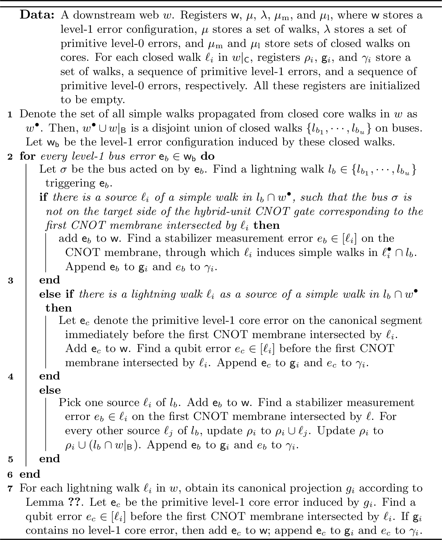
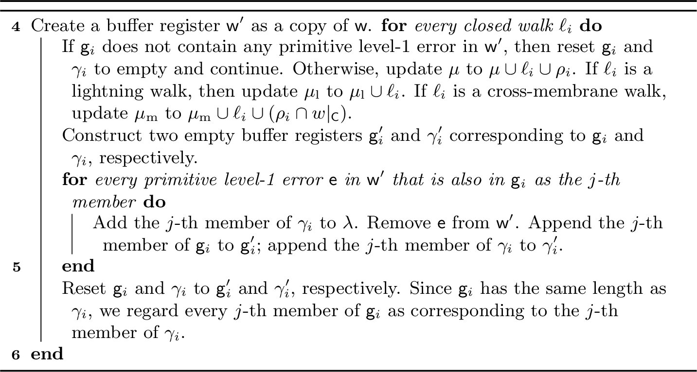
We now bound the weight of physical errors in \(\mu\) to prove condition (iii). We first note that every closed walk \(\ell_{i}\) (on a core) in \(w\) is a simple walk; the corresponding register \(\mathsf{g}_i\) is non-empty if and only if \(\ell_i\) is added to \(\mu\) during the fourth step of Algorithm 14. For each lightning walk \(\ell_i\) in \(w\) on a core with a non-empty register \(\mathsf{g}_{i}\), the number of primitive bus errors in \(\mathsf{g}_i\), if non-zero, is strictly smaller than the number of membranes intersected by \(\ell_i\). Moreover, \(\mathsf{g}_i\) contains at most one primitive core error. Thus, the weight of stabilizer measurement errors in \(\ell_i\), \(|\ell_{i,\perp}|\), is lower bounded by \(d_0(|\mathsf{g}_i|-1)\); and the weight of qubit errors in \(\ell_i\), \(|\ell_{i,||}|\), is lower bounded by \(d_0\). Thus, the weight of \(\ell_{i}\), \(|\ell_{i}|\), is lower bounded by \(d_0|\mathsf{g}_i|\). Let \(\mathsf{w}_{\mathrm{lc}}\) be the sum of the register \(\mathsf{g}_i\) for every lightning core walk \(\ell_i\) in \(w\). Thus, we can bound the weight of \(\mu_{\mathrm{l}}\) (contributed by lightning walks on cores in step 4 of Algorithm 14) as follows: \[\label{eq:32bound32on32lightning32walk32error} d_{0}|\mathsf{w}_{\mathrm{lc}}|\leq |\mu_{\mathrm{l}}|.\tag{2}\]
Consider a primitive level-1 error \(\mathsf{e}_{b}\) in \(\mathsf{w}\backslash\mathsf{w}_{\mathrm{lc}}\). We know that \(\mathsf{e}_{b}\) is a bus error contained in the level-1 error register \(\mathsf{g}_{j}\) of some cross-membrane walk \(\ell_j\) in \(w\). We say \(\mathsf{e}_{b}\) is a leading bus error if the \(Z\) bus acted on by \(\mathsf{e}_{b}\) is on the target side of the core-bus CNOT gate corresponding to the first CNOT membrane intersected by \(\ell_{j}\). Otherwise, we say \(\mathsf{e}_b\) is a trailing bus error. If the level-1 error register \(\mathsf{g}_{j}\) of \(\ell_j\) contains no leading bus error, then the weight of stabilizer measurement errors in \(\ell_j\), \(|\ell_{j,\perp}|\), is lower bounded by \(d_0|\mathsf{g}_j|\). On the other hand, if \(\mathsf{g}_i\) contains a leading bus error \(\mathsf{e}_{b}\), then \(|\ell_{j,\perp}|\) is lower bounded by \(d_0(|\mathsf{g}_{j}|-1)\). According to Algorithm 14, we have picked a lightning walk \(l_{b}\) on a \(Z\) bus that induces \(\mathsf{e}_{b}\). Let \(\xi_{b}\subset\{\ell_1,\cdots,\ell_{r}\}\) be the collection of all sources of simple walks in \(l_{b}\cap w^{\bullet}\). We say \(\xi_b\) is the source set corresponding to \(\mathsf{e}_{b}\). Then, Algorithm 14 guarantees that \(\mu\) contains \(\xi_{b}\) and \(l_{b}\cap w|_{\mathsf{B}_{\blacktriangledown}}\). According to Lemma 4, the weight of simple walks, \(|\ell_{b}\cap w^{\bullet}|\), is upper bounded by \(|\xi_{b,||}|\)/2. MWPM decoding ensures that \(|l_{b}\cap w_{\kappa}|\leq |l_{b}\cap w_{\epsilon}|+|l_{b}\cap w^{\bullet}|\). From these two inequalities, we obtain the following bounds: \[\begin{align} \label{eq:32single32error32bound32on32qubit32errors32in32cm32core32walks} |(l_{b}\cap w|_{\mathsf{B}_{\blacktriangledown}})|\leq& 2|l_b\cap w_{\epsilon}| + |\xi_{b,||}|/2, \nonumber\\ d_0\leq |l_{b}|\leq& 2|l_b\cap w_{\epsilon}| + |\xi_{b,||}|. \end{align}\tag{3}\] Let \(\mathsf{w}_{\mathrm{tb}}\) and \(\mathsf{w}_{\mathrm{lb}}\) be the collection of trailing bus errors and the collection of leading bus errors in \(\mathsf{w}\backslash\mathsf{w}_{\mathrm{lc}}\), respectively. Then, the total weight of stabilizer measurement errors in \(\mu_{\mathrm{m}}\), \(|\mu_{\mathrm{m},\perp}|\) has a lower bound: \[\label{eq:32lower32bound32stab32error32in32cm32walks} d_{0}|\mathsf{w}_{\mathrm{tb}}|\leq |\mu_{\mathrm{m},\perp}|.\tag{4}\] As the source sets corresponding to primitive errors in \(\mathsf{w}_{\mathrm{lb}}\) are mutually disjoint, we can extend Eq. 3 to obtain the following inequalities. \[\begin{align} \label{eq:32bound32on32qubit32errors32in32all32cm32core32walks} |\mu\cap w|_{\mathsf{B}_{\blacktriangledown}}| \leq& 2|(\mu\cap w_{\epsilon}|_{\mathsf{B}_{\blacktriangledown}})| + |\mu_{\mathrm{m},||}|/2 ,\nonumber\\ d_0|\mathsf{w}_{\mathrm{lb}}|\leq& 2|(\mu\cap w_{\epsilon}|_{\mathsf{B}_{\blacktriangledown}})| + |\mu_{\mathrm{m},||}|. \end{align}\tag{5}\] We now bound the weight of physical errors in \(\mu\) in terms of the weight of level-1 errors \(|\mathsf{w}|\). \[\begin{align} |\mu\cap w_{\epsilon}|=&|\mu_{\mathrm{l}}\cap w_{\epsilon}|+ |\mu_{\mathrm{m}}\cap w_{\epsilon}| + |(\mu|_{\mathsf{B}_{\blacktriangledown}}\cap w_{\epsilon})|\nonumber\\ \geq& \frac{1}{2}(|\mu_{\mathrm{l}}|+|\mu_{\mathrm{m},\perp}|+|\mu_{\mathrm{m},||}|+2|(\mu|_{\mathsf{B}_{\blacktriangledown}}\cap w_{\epsilon})|)\nonumber\\ \geq& \frac{d_0}{2}(|\mathsf{w}_{\mathrm{lc}}|+|\mathsf{w}_{\mathrm{tb}}|+|\mathsf{w}_{\mathrm{lb}}|)=d_{0}|\mathsf{w}|/2, \end{align}\] where the first inequality is implied by MWPM decoding; the second inequality is derived from Eq 2 , Eq. 4 , and Eq. 5 . Similarly, we can bound \(|\mu\cap w_{\epsilon}|\) by \(|\mu|\) as follows. \[|\mu\cap w_{\epsilon}| \geq \frac{1}{2}(|\mu_{\mathrm{l}}|+|\mu_{\mathrm{m},\perp}|+|\mu_{\mathrm{m},||}|/2+|(\mu|_{\mathsf{B}_{\blacktriangledown}})|\geq \frac{1}{4}|\mu|.\] ◻
Building on Lemma 6, we can now bound \(f\).
Lemma 7 (Bounds on a residual level-0 error configuration). Consider the level-0 residual error configuration \(f\) (consisting only of \(X\) errors). Denote the collection of physical errors in \(f\) as \(f_{\epsilon}\) and the collection of inferred errors in \(f\) as \(f_{\kappa}\). We can explicitly construct a level-1 error \(\mathsf{f}=\mathsf{e}_1+\mathsf{e}_2+\cdots+\mathsf{e}_{|\mathsf{f}|}\), where each \(\mathsf{e}_{i}\) is a distinct primitive level-1 error, such that \(f\) induces the level-1 error \(\mathsf{f}\). Moreover, we can find two level-0 error configurations \(\lambda_f\subset\mu_f\subset f\) such that (i) \(\lambda_f=e_1+\cdots+e_{|\mathsf{f}|}\) with each \(e_{i}\) a distinct primitive level-0 error in the receptive zone of \(\mathsf{e}_{i}\), (ii) each connected component of \(\mu_f\) (on the level-0 adjacency graph) contains at least one element in \(\lambda_f\), and (iii) the weight of physical errors in \(\mu_f\), \(|\mu_f\cap f_{\epsilon}|\), is lower bounded by \(\max(|\mu_f|/4,d_0|\mathsf{f}|/2)\).
Proof.
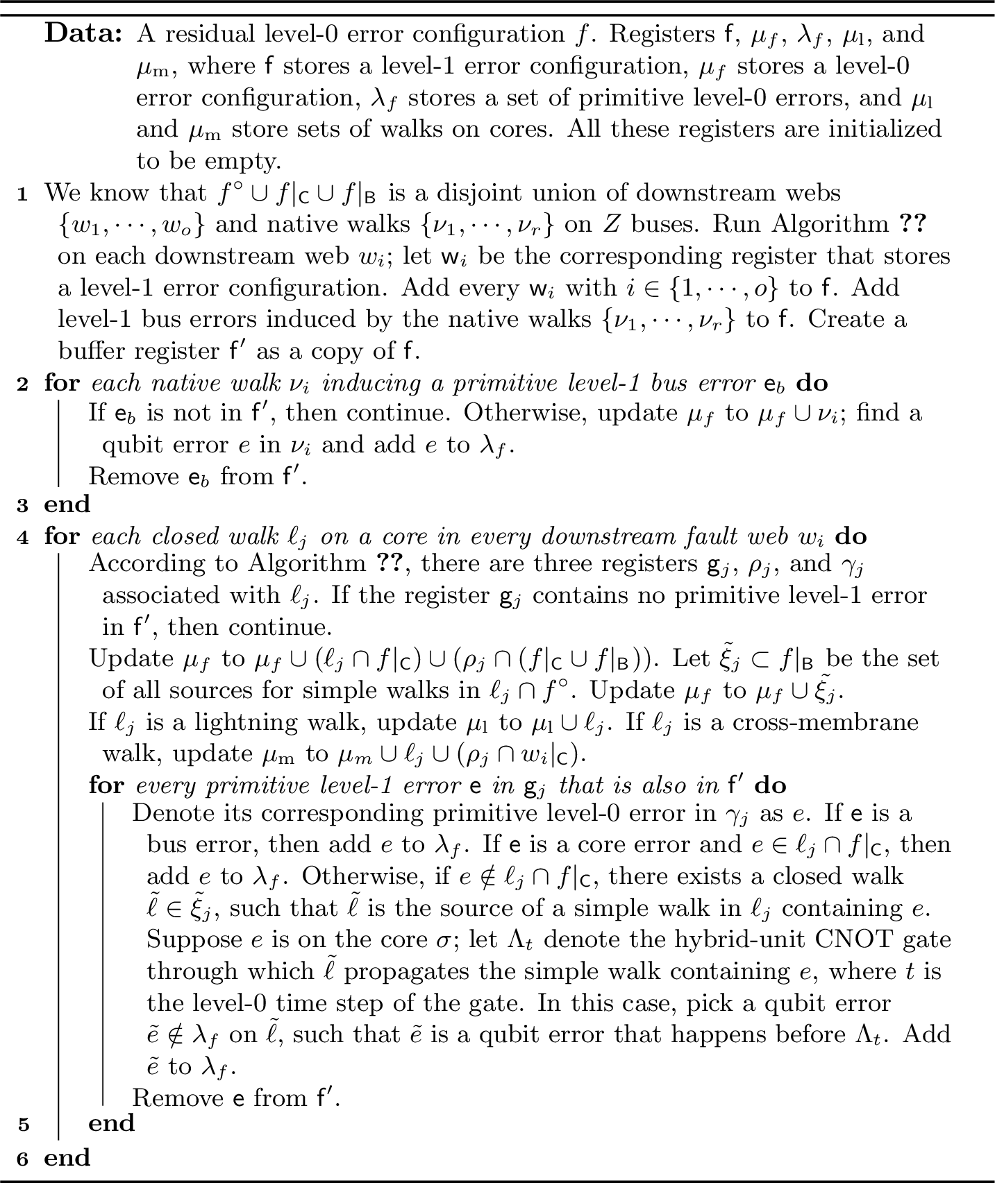
We construct \(\mathsf{f}\), \(\mu_{f}\), and \(\lambda_{f}\) explicitly by running Algorithm 16. We now bound the weight of physical errors in \(f\). Following the definitions introduced in the proof of Lemma 6, we let \(\mathsf{f}_{\mathrm{lc}}\) denote the collection of level-1 errors in \(\mathsf{f}\) contributed by lightning walks in \(\mu_{\mathrm{l}}\); let \(\mathsf{f}_{\mathrm{lb}}\) and \(\mathsf{f}_{\mathrm{tb}}\) denote the collections of leading bus errors and trailing bus errors in \(\mathsf{f}\), respectively; let \(\mathsf{f}_{\mathrm{nb}}\) denote the collection of level-1 bus errors in \(\mathsf{f}\) induced by native walks on \(Z\) buses. According to Algorithm 16, \(\mu_{\mathrm{l}}\) is a disjoint union of lightning walks on cores; \(\mu_{\mathrm{m}}\) is a disjoint union of cross-membrane walks on cores. For errors in \(\mu_{f}|_{\mathsf{B}_{\blacktriangledown}}\), we have the following two bounds following the same argument for Eq. 5 . \[\begin{align} \label{eq:32bound32f32cm32and32downstream32walks} |(\mu_{f}|_{\mathsf{B}_{\blacktriangledown}})|\leq& 2|(\mu_{f}|_{\mathsf{B}_{\blacktriangledown}}\cap f_{\epsilon})| + |\mu_{\mathrm{m},||}|/2, \nonumber \\ d_0(|\mathsf{f}_{\mathrm{lb}}|+|\mathsf{f}_{\mathrm{nb}}|)\leq& 2|(\mu_{f}|_{\mathsf{B}_{\blacktriangledown}}\cap f_{\epsilon})| + |\mu_{\mathrm{m},||}|. \end{align}\tag{6}\] Following Eq. 2 and Eq. 4 , we have similar bounds on \(|\mu_{\mathrm{m},\perp}|\) and \(|\mu_{\mathrm{l}}|\): \[\begin{align} \label{eq:32bound32f32cm32walks32with32lv132errors} d_0|\mathsf{f}_{\mathrm{tb}}|\leq& |\mu_{\mathrm{m},\perp}| \nonumber\\ d_0|\mathsf{f}_{\mathsf{lc}}|\leq& |\mu_{\mathrm{l}}| \end{align}\tag{7}\] As we are eventually interested in bounding error weights for \(\mu_{f}\), we would like to relate bounds on \(\mu_{\mathrm{l}}\) and \(\mu_{\mathrm{m}}\) to bounds on \(\mu_{f}\). Since the total weight of propagated simple walks on cores from \(\mu_{f}\) is upper bounded by \(|(\mu_f|_{\mathsf{B}_{\lozenge}})|/2\), we have the following two inequalities: \[\begin{align} |\mu_{\mathrm{l}}|+|\mu_{\mathrm{m}}|\leq& |(\mu_f|_{\mathsf{C}})| + |(\mu_f|_{\mathsf{B}_{\lozenge}})|/2,\nonumber \\ |(\mu_{f}|_{\mathsf{C}}\cap f_{\kappa})| \leq& |(\mu_{f}|_{\mathsf{C}}\cap f_{\epsilon})| + |(\mu_f|_{\mathsf{B}_{\lozenge}})|/2, \end{align}\] which can be reorganized into the following bounds: \[\begin{align} \label{eq:32bound32f32cm32walks} |(\mu_{f}|_{\mathsf{C}})|\leq& 2|(\mu_{f}|_{\mathsf{C}}\cap f_{\epsilon})|+|(\mu_{f}|_{\mathsf{B}_{\lozenge}})|/2,\nonumber\\ |\mu_{\mathrm{l}}|+|\mu_{\mathrm{m}}|\leq& 2|(\mu_{f}|_{\mathsf{C}}\cap f_{\epsilon})|+|(\mu_{f}|_{\mathsf{B}_{\lozenge}})|. \end{align}\tag{8}\] Also, MWPM decoding on \(\mathcal{G}_{\mathsf{B}_{\lozenge}}\) implies \(|(\mu_{f}|_{\mathsf{B}_{\lozenge}})|\leq 2|(\mu_{f}|_{\mathsf{B}_{\lozenge}}\cap f_{\epsilon})|\). Thus, we can bound the weight of physical errors in \(\mu_f\) by the weight of the level-1 error configuration \(\mathsf{f}\) as follows. \[\begin{align} |\mu_f\cap f_{\epsilon}|=& |(\mu_{f}|_{\mathsf{B}_{\lozenge}}\cap f_{\epsilon})| + |(\mu_{f}|_{\mathsf{C}}\cap f_{\epsilon})| + |(\mu_{f}|_{\mathsf{B}_{\blacktriangledown}}\cap f_{\epsilon})|\nonumber\\ \geq& |(\mu_{f}|_{\mathsf{B}_{\lozenge}})|/2 + |(\mu_{f}|_{\mathsf{C}}\cap f_{\epsilon})| + |(\mu_{f}|_{\mathsf{B}_{\blacktriangledown}}\cap f_{\epsilon})|\nonumber\\ \geq& (|\mu_{\mathrm{l}}|+|\mu_{\mathrm{m}}|)/2+ |(\mu_{f}|_{\mathsf{B}_{\blacktriangledown}}\cap f_{\epsilon})|\nonumber\\ \geq&\frac{d_0}{2}(|\mathsf{f}_{\mathrm{lc}}|+|\mathsf{f}_{\mathrm{lb}}|+|\mathsf{f}_{\mathrm{tb}}|+|\mathsf{f}_{\mathrm{nb}}|) = d_0|\mathsf{f}|/2, \end{align}\] where we use Eq. 8 for the second inequality, and Eq. 6 and Eq. 7 for the last inequality. Similarly, we now bound \(|\mu_{f}\cap f_{\epsilon}|\) in terms of the weight of \(\mu_{f}\). \[\begin{align} |\mu_{f}\cap f_{\epsilon}|\geq& \big(|(\mu_{f}|_{\mathsf{B}_{\lozenge}})|/4 + |(\mu_{f}|_{\mathsf{C}})|/4+|\mu_{\mathrm{m}}|/8 \nonumber\\ & + |(\mu_{f}|_{\mathsf{B}_{\blacktriangledown}}\cap f_{\epsilon})|\nonumber\big) \\ \geq& (|(\mu_{f}|_{\mathsf{B}_{\lozenge}})|+|(\mu_{f}|_{\mathsf{C}})|+|(\mu_{f}|_{\mathsf{B}_{\blacktriangledown}})|)/4=|\mu_{f}|/4. \end{align}\] ◻
We previously considered only level-0 \(X\) error configurations in this subsection. Now, we allow \(f\) to be a general level-0 residual error configuration with \(f=\epsilon+\kappa\), where \(\epsilon\in\mathbb{Z}_2^{|\mathcal{E}_{\mathrm{dep}}|}\) is the physical error term and \(\kappa\in\mathbb{Z}_2^{|\mathcal{E}_{0}|}\) is the inferred error configuration. Let \(f_{\epsilon}:=f\cap \epsilon\) and \(f_{\kappa}:=f\cap\kappa\), representing physical errors and inferred errors in \(f\), respectively. Consider the \(X\)-basis projection \(f_{X}=\epsilon_{X}+\kappa_{X}\). In previous arguments, \(f_{X,\epsilon}:=f_{X}\cap\epsilon_{X}\) and \(f_{X,\kappa}:=f_{X}\cap\kappa_{X}\) represent physical errors and inferred errors in \(f_{X}\), respectively. We define similar notations for \(f_Z\). To relate subconfigurations in \(f_X\cup f_{Z}\) to subconfigurations in \(f\), we construct a section map \(\mathbb{S}_{f}\) that maps every subset (subconfiguration) in \(f_{X}\cup f_{Z}\) to a subset (subconfiguration) in \(f\) with the following four properties.
For each subconfiguration \(g\subset f_{X}\cup f_{Z}\), \(\mathbb{S}_{f}(g)=\bigcup_{e\in g} \mathbb{S}_{f}(e)\) with each \(e\) a primitive level-0 error in \(g\).
For each primitive error \(e_{X}\in f_{X}\), \(\mathbb{P}_{X}\circ \mathbb{S}_f(e_X)=e_X\). Similarly, for each primitive error \(e_{Z}\in f_{Z}\), \(\mathbb{P}_{Z}\circ \mathbb{S}_f(e_Z)=e_Z\).
For every \(g_X\subset f_{X,\epsilon}\), \(\mathbb{S}_{f}(g_X)\subset f_{\epsilon}\). For every \(g_X\subset f_{X,\kappa}\), \(\mathbb{S}_f(g_X)\subset f_{\kappa}\).
For every \(g_{Z}\subset f_{Z,\epsilon}\), \(\mathbb{S}_{f}(g_Z)\subset f_{\epsilon}\). For every \(g_Z\subset f_{Z,\kappa}\), \(\mathbb{S}_f(g_Z)\subset f_{\kappa}\).
By construction, we know that given a subconfiguration \(g\subset f_{X}\cup f_{Z}\), \(|\mathbb{S}_f(g)\cap \epsilon|\geq \max(|g_X\cap \epsilon_X|,|g_{Z}\cap\epsilon_{Z}|)\). Additionally, if \(g\) forms a connected cluster on the level-0 adjacency graph, then \(\mathbb{S}_{f}(g)\) also forms a connected cluster. Building on Lemma 7, we can bound a general level-0 residual error configuration.
Lemma 8 (Bounds on a general level-0 residual error configuration). Consider the general level-0 residual error configuration \(f\). We can explicitly construct a level-1 \(X\) error \(\mathsf{f_X}=\mathsf{e}_1+\mathsf{e}_2+\cdots+\mathsf{e}_{|\mathsf{f}|}\), where each \(\mathsf{e}_{i}\) is a distinct primitive level-1 \(X\) error, such that \(f_X\) induces the level-1 error \(\mathsf{f_X}\). Moreover, we can find two general level-0 error configurations \(\lambda_f\subset\mu_f\subset f\) such that (i) \(\lambda_f=e_1+\cdots+e_{|\mathsf{f_X}|}\) with each \(e_{i}\) a distinct primitive level-0 error whose \(X\)-basis projection is in the receptive zone of \(\mathsf{e}_{i}\), (ii) each connected component of \(\mu_f\) (on the level-0 adjacency graph) contains at least one element in \(\lambda_f\), and (iii) the weight of physical errors in \(\mu_f\), \(|\mu_f\cap \epsilon|\), is lower bounded by \(\max(|\mu_f|/4,d_0|\mathsf{f_X}|/2)\).
Proof. According to Lemma 7, we construct \(\mathsf{f}_{\mathsf{X}}\) from \(f_X\) and find \(\lambda_{f_X}\subset\mu_{f_X}\subset f_{X}\) satisfying all three conditions in Lemma 7. Let \(\lambda_f:=\mathbb{S}_{f}(\lambda_{f_X})\) and \(\mu_{f}:=\mathbb{S}_{f}(\mu_{f_X})\). Then, these two general error configurations satisfy all requirements in this lemma. ◻
We follow previous fault-tolerance proofs [7], [72], [73] (in particular, the ‘bad set’ formalism in Ref. [73]) to provide a sufficient condition for upper bounding level-1 error probabilities.
Lemma 9 (Sufficient condition for upper bounding a level-1 error probability). Consider a level-1 error \(\mathsf{g}\). Suppose there exists a collection of general level-0 error configurations \(\mathcal{F}_{\mathsf{g}}\), referred to as the key collection of \(\mathsf{g}\), that satisfies the following conditions
For each general residual level-0 error configuration \(f\) (composed of two components, physical errors \(f_{\epsilon}\) and decoded errors \(f_{\kappa}\), respectively) that induces a level-1 error configuration containing \(\mathsf{g}\), there exists \(\mu\in\mathcal{F}_{\mathsf{g}}\) with \(\mu\subset f\) such that the weight of the intersection of \(\mu\) and the physical errors in \(f\) is lower bounded by both \(d_{0}|\mathsf{g}|/2\) and \(|\mu|/C_1\), where \(C_1>1\) is a constant independent of \(f\).
The number of error configurations in \(\mathcal{F}_{\mathsf{g}}\) with a weight \(\mathrm{w}\) is upper bounded by \(C_{2}\cdot C_{3}^{\mathrm{w}}\), where both \(C_2>0\) and \(C_{3}>1\) are constants. Every error configuration in \(\mathcal{F}_{\mathsf{g}}\) has a weight at least \(d_{0}|\mathsf{g}|/2\).
Moreover, suppose physical level-0 errors are local stochastic, such that the event of physical errors containing a general level-0 error configuration \(\epsilon\) may occur with a probability upper bounded by \(p^{|\epsilon|}\), with \(p\leq 1/(4C_3)^{C_1}\). Then, the level-1 error \(\mathsf{g}\) occurs with probability upper bounded by \(C_A(p/p_{th})^{d_{0}|\mathsf{g}|/2}\), where \(C_{A}:=3C_2C_3/(C_3-1)\) and \(p_{th}:=(1/(2C_3)^{C_1})\).
Proof. Define event \(\Upsilon_{\mathsf{g}}\) as the set of all general level-0 physical-error configurations for which the physical-error configuration and the corresponding inferred level-0 error configuration jointly induce a level-1 error configuration containing \(\mathsf{g}\). Therefore, the probability that \(\mathsf{g}\) occurs at level 1 is equal to the level-0 probability of \(\Upsilon_{\mathsf{g}}\).
From the key collection \(\mathcal{F}_{\mathsf{g}}\), we define the set of key errors \(\Xi:=\{\xi|\xi\subset \mu\;\text{for some}\; \mu\in\mathcal{F}_{\mathsf{g}}\;\text{with}\;|\xi|\geq d_0|\mathsf{g}|\;\text{and}\;|\xi|\geq |\mu|/C_1\}\). For a general level-0 error configuration \(\xi\), define \(\hat{\xi}:=\{f|\xi\subset f\}\) as the collection of all general level-0 error configurations containing \(\xi\). For any \(\epsilon\in\Upsilon_{\mathsf{g}}\), let \(\kappa\) be the inferred level-0 error configuration from level-0 decoding with an input level-0 syndrome configuration \(\partial_{0}\epsilon\). According to the first condition in the lemma, there exists \(\xi\in\Xi\) such that \(\xi\subset\epsilon\) (or equivalently, \(\epsilon\in\hat{\xi}\)). Thus, the event \(\Upsilon_{\mathsf{g}}\) is contained in the event \(\hat{\Xi}:=\bigcup_{\xi\in\Xi}\hat{\xi}=\bigcup_{\mu\in\mathcal{F}_{\mathsf{g}}}\left(\bigcup_{\xi\in\Xi,\;\xi\subset\mu}\hat{\xi}\right)\). Notice that for every \(\mu\in\mathcal{F}_{\mathsf{g}}\), the probability \[\begin{align} P\left(\bigcup_{\xi\in\Xi,\;\xi\subset\mu}\hat{\xi}\right)\leq& \sum_{\xi\in\Xi,\;\xi\subset\mu}p^{\max(d_0|\mathsf{g}|/2,|\mu|/C_1)} \nonumber\\ \leq& (2^{C_1}p)^{\max(d_0|\mathsf{g}|/2,|\mu|/C_1)}, \end{align}\] where the second inequality is based on the observation that the number of summations is upper bounded by \(2^{|\mu|}\). Therefore, we can bound the level-1 error probability \(P(\Upsilon_{\mathsf{g}})\) as follows: \[\begin{align} P(\Upsilon_{\mathsf{g}})\leq& P(\hat{\Xi})\leq \sum_{\mu\in\mathcal{F}_{\mathsf{g}}} (2^{C_1}p)^{\max(d_0|\mathsf{g}|/2,|\mu|/C_1)}\nonumber\\ \leq& \sum_{\mathrm{w}=\lceil d_0|\mathsf{g}|/2\rceil}^{\infty} (2^{C_1}p)^{\max(d_0|\mathsf{g}|/2,\mathrm{w}/C_1)}\cdot C_2C_3^{\mathrm{w}}\nonumber\\ \leq& \frac{3C_2C_3}{C_3-1}\left(\frac{p}{1/(2C_3)^{C_1}}\right)^{d_{0}|\mathsf{g}|/2}. \end{align}\] Here, the third inequality follows from the second condition in the lemma, and the last inequality uses \(p\leq1/(4C_3)^{C_1}\). ◻
We will need the following lemma from Ref. [72] (widely used in fault-tolerance proofs to count the number of errors) to upper bound the number of elements of a certain weight in a set of error configurations.
Lemma 10 (Counting lemma [72]). Consider a graph \(G\) in which every vertex has a degree of at most \(r\). Given a non-empty set \(\lambda\) of vertices in \(G\), let \(\Sigma_{m}(\lambda)\) be the collection of all sets of vertices satisfying the following conditions.
The set contains exactly \(m\) vertices.
The set contains \(\lambda\) as a subset.
Every connected cluster of the set (on \(G\)) contains at least one element in \(\lambda\).
Then, the number of sets in \(\Sigma_{m}(\lambda)\) is upper bounded by \(\mathfrak{e}^{|\lambda|-1}(r\mathfrak{e})^{m-|\lambda|}\), where \(\mathfrak{e}\) is Euler’s number.
We note that for our level-0 adjacency graph \(\mathcal{A}\), the degree of any vertex is upper bounded by \(48\), since each primitive level-0 error triggers up to \(4\) level-0 detectors, and each level-0 detector can be triggered by up to \(12\) distinct level-0 error locations.
Theorem 2 (Approximate error reduction theorem). Consider a level-0 circuit composed of level-0 SE rounds on cores and shuttle buses and X- and \(Z\)-basis readout gadgets. Every core has a distance of \(d_{0}\); every shuttle bus has a width of \(d_{0}\) and a length of \(d_{0}d_{1}\). Compilation parameter \(\alpha_{\mathsf{b}}\) is set as \(d_1\). We further assume perfect time boundaries for cores for simplicity. Suppose we are only interested in the results of a subset \(\mathcal{M}_1\) of readout gadgets, such that the separation between every two \(X\)-basis (or \(Z\)-basis) readout gadgets in \(\mathcal{M}_1\) is at least \(d_{0}\). We construct level-1 error locations for \(\mathcal{M}_1\) according to the procedure in Sec. 1.6. Let \(\tau_{\mathsf{c}}\) denote the maximum length for a canonical segment on cores; let \(\tau_{\mathsf{b}}\) denote the maximum lifetime for a shuttle bus. Let \(|\mathsf{b}|\) be the number of shuttle buses used in the circuit. Then, under the phenomenological depolarizing noise model with an error rate \(p<1/(4r\mathfrak{e})^{4}\) at level 0, except for a rare event with a probability upper bounded by \(\mathrm{v}_{\mathsf{b}}(p/\sqrt{p_{th}})^{d_0d_2/2}\), the induced level-1 \(X\) (or \(Z\)) errors are local stochastic with a level-1 error rate upper bounded by \(z_{\mathrm{max}}(p/p_{th})^{d_{0}/2}\). Here, \(\mathrm{v}_{\mathsf{b}}:=\tau_{\mathsf{b}}d_{0}^2d_{1}|\mathsf{b}|\), \(p_{th}:=1/(2r\mathfrak{e})^4\), \(z_{\mathrm{max}}:=16\max(\tau_{\mathsf{c}},\tau_{\mathsf{b}}) d_{0}^3d_{1}^2\), and \(r=48\), which upper bounds the vertex degrees of the level-0 adjacency graph.
Proof. Without loss of generality, we focus on level-1 \(X\) errors in the proof. First, consider the event \(\mathcal{B}_{d_1}\) that a general level-0 residual error configuration induces an \(X\)-basis cycle on an \(X\) bus of weight at least \(d_{0}d_{1}\). Let \(\mathcal{H}_{\mathrm{w}}\) be the set of all weight-\(\mathrm{w}\) general level-0 error configurations whose \(X\)-basis restriction is a weight-\(\mathrm{w}\) cycle on an \(X\) bus. Then, according to Lemma 10, \(|\mathcal{H}_{\mathrm{w}}|\) is upper bounded by \((4d_{0}^2d_{1}\cdot\tau_{\mathsf{b}}\cdot|\mathsf{b}|)\cdot (r\mathfrak{e})^{\mathrm{w}-1}\), where the first factor upper bounds the number of level-0 error locations on \(X\) buses and the second factor upper bounds the number of weight-\(\mathrm{w}\) clusters on the level-0 adjacency graph \(\mathcal{A}\) containing a fixed level-0 error location on an \(X\) bus. The probability of inducing any given general level-0 error configuration in \(\mathcal{H}_{\mathrm{w}}\) is upper bounded by \(p^{\mathrm{w}/2}2^{\mathrm{w}}\). Thus, the probability of the event \(\mathcal{B}_{d_1}\) is upper bounded as \[\begin{align} P(\mathcal{B}_{d_1})\leq& \frac{4d_0^2d_1\cdot\tau_{\mathsf{b}}\cdot|\mathsf{b}|}{r\mathfrak{e}} \sum_{\mathrm{w=d_{0}d_{1}}}^{\infty}(2r\mathfrak{e} \sqrt{p})^{\mathrm{w}} \nonumber \\ =& \frac{4d_0^2d_1\cdot \tau_{\mathsf{b}}\cdot|\mathsf{b}|}{r\mathfrak{e}(1-2r\mathfrak{e}\sqrt{p})}\left((2r\mathfrak{e})^2p\right)^{d_{0}d_{1}/2}\nonumber\\ \leq& \mathrm{v}_{\mathsf{b}}\left(p/\sqrt{p_{th}}\right)^{d_{0}d_{1}/2}. \end{align}\] We exclude this event in the following.
For a level-1 \(X\) error configuration \(\mathsf{g}\), define \(\mathcal{F}_{\mathsf{g}}\) as a collection of all general level-0 error configurations satisfying the following conditions:
The general level-0 error configuration has a weight of at least \(d_0|\mathsf{g}|\)/2.
The general level-0 error configuration contains a weight-\(|\mathsf{g}|\) subconfiguration \(\lambda\), such that each primitive level-1 error \(\mathsf{e}\) in \(\mathsf{g}\) corresponds to a distinct primitive level-0 error in \(\lambda_X\) in the receptive zone of \(\mathsf{e}\).
Each connected component (on the level-0 adjacency graph) of the general level-0 error configuration contains at least one element in \(\lambda\).
The size of the receptive zone (the number of level-0 error locations whose \(X\)-basis restriction is contained in the zone) of a primitive level-1 core error is upper bounded by \(2\tau_{c}\cdot 4d_{0}^2(1+d_{0}d_{1}^2)\leq 16\tau_{c}d_{0}^3 d_{1}^{2}\). The size of the receptive zone of a primitive level-1 bus error is upper bounded by \(4\tau_{\mathsf{b}}d_{0}^{2}d_{1}+\tau_{\mathsf{b}}d_{0}^2\leq 8\tau_{\mathsf{b}}d_{0}^2d_{1}\). Then, we can simply upper bound the size of any receptive zone by \(z_{\mathrm{max}}\). Denote the number of weight-\(\mathrm{w}\) configurations in \(\mathcal{F}_{\mathsf{g}}\) as \(C_{\mathsf{g}}(\mathrm{w})\). According to Lemma 10, \(C_{\mathsf{g}}(\mathrm{w})\leq (z_{\mathrm{max}}/r)^{|\mathsf{g}|}(r\mathfrak{e})^{\mathrm{w}}\). Combining this bound with Lemma 8, we can see that \(\mathcal{F}_{\mathsf{g}}\) is a key collection of \(\mathsf{g}\) in Lemma 9. Then, the probability of inducing \(\mathsf{g}\), \(P(\mathsf{g})\), is upper bounded as follows. \[P(\mathsf{g})\leq z_{\mathrm{max}}^{|\mathsf{g}|} \cdot \left(p/p_{th}\right)^{d_{0}|\mathsf{g}|/2}\] Thus, the distribution of induced level-1 errors is local stochastic with a level-1 error probability upper bounded by \(z_{\mathrm{max}} \left(p/p_{th}\right)^{d_{0}/2}\). ◻
3 Logical Pauli measurements↩︎
In this section, we analyze the performance of the LMSs constructed for measuring logical \(X\) and \(Z\) operators on an HLP. We then describe how to measure general logical Pauli operators with \(H\)-transformed and \(HS\)-transformed readout gadgets. We extend our analysis on the induced level-1 error model as well as LMSs to incorporate \(H\)-transformed gadgets. Finally, we extend hybrid-unit CNOT gates to enable transversal CNOT gates between shuttle buses and external cores. We tentatively propose a hybrid architecture where an HLP or possibly multiple HLPs work closely with external cores to run logical computation.
3.1 Performance analysis of LMSs for measuring logical \(X\) and \(Z\) operators↩︎
We first consider a single LMS consisting of \(d_{1}\) \(X\)-basis (or \(Z\)-basis) readout gadgets. Let \(\mathcal{M}\) be the collection of all logical readout gadgets in the LMS and all readout gadgets for level-1 SE. We construct a level-1 error model for \(\mathcal{M}\). We can lower bound the number of primitive level-1 errors required to trigger a logical measurement error in this LMS.
Lemma 11 (Lower bound on the level-1 distance for an LMS). Given the level-1 error model for \(\mathcal{M}\), for a level-1 error configuration \(\mathsf{f}\) with \(\partial_{1}\mathsf{f}=0\), if \(|\mathsf{f}|\) is smaller than \(d_1\), then \(\mathsf{f}\) does not induce a logical measurement error on the LMS.
Proof. Define an adjacency graph \(\mathcal{A}_{1}\), with a vertex set of all primitive level-1 errors, such that two vertices are connected by an edge if and only if the corresponding level-1 errors have overlapping level-1 syndromes. Without loss of generality, we assume \(\mathsf{f}\) is a connected cluster on \(\mathcal{A}_1\). Let \(\mathsf{D}_{\mathsf{S}}\) be the set of all level-1 detectors generated by level-1 SE. Let \(\overline{\partial}_{1\mathsf{S}}\) be the projection of the level-1 syndrome map onto \(\mathsf{D}_{\mathsf{S}}\). Define another adjacency graph \(\mathcal{A}_{\mathsf{S}}\), with a vertex set of all primitive level-1 errors on cores and buses for level-1 SE, such that two vertices \(\mathsf{e}_{1}\) and \(\mathsf{e}_{2}\) (corresponding to two primitive level-1 errors) are connected by an edge if and only if \(\overline{\partial}_{1\mathsf{S}}\mathsf{e}_1\cap\overline{\partial}_{1\mathsf{S}}\mathsf{e}_{2}\neq \emptyset\). The level-1 error configuration \(\mathsf{f}\) is composed of two components: a configuration \(\mathsf{f}_{\mathsf{S}}\) of level-1 errors on cores and buses for level-1 SE and a configuration \(\mathsf{f}_{\mathsf{R}}\) of level-1 errors on buses in the LMS. We can see that \(\overline{\partial}_{1\mathsf{S}}\mathsf{f}_{\mathsf{S}}=\overline{\partial}_{1\mathsf{S}}\mathsf{f}=0\). Thus, we can decompose \(\mathsf{f}_{\mathsf{S}}\) into a series of level-1 error configurations \(\mathsf{f}_{\mathsf{S},1},\cdots,\mathsf{f}_{\mathsf{S},j}\), such that each \(\mathsf{f}_{\mathsf{S},i}\) (\(i\in\{1,\cdots,j\}\)) is a connected cluster on \(\mathcal{A}_{\mathsf{S}}\) with \(\overline{\partial}_{1\mathsf{S}}f_{\mathsf{S},i}=0\).
For each \(\mathsf{f}_{\mathsf{S},i}\) (\(i\in\{1,\cdots,j\}\)), denote the smallest and the largest level-1 time coordinates of detectors triggered by primitive errors in \(\mathsf{f}_{\mathsf{S},i}\) as \(\mathsf{t}_{i,0}\) and \(\mathsf{t}_{i,1}\), respectively. We know that for every integer \(\mathsf{t}\) with \(\mathsf{t}_{i,0}\leq \mathsf{t}\leq \mathsf{t}_{i,1}-1\), there is at least one primitive error in \(\mathsf{f}_{\mathsf{S},i}\) such that the level-1 detectors triggered by the error in \(\mathsf{D}_{\mathsf{S}}\) cover both time coordinates \(\mathsf{t}\) and \(\mathsf{t}+1\). Thus, the weight of primitive errors (in \(\mathsf{f}_{\mathsf{S},i}\)) whose syndromes have two different time coordinates is lower bounded by \(\mathsf{t}_{i,1}-\mathsf{t}_{i,0}\). We then back propagate all primitive level-1 core errors in \(\mathsf{f}_{\mathsf{S},i}\) back to the beginning of the level-1 SE round \(\mathsf{t}_{i,0}\) and denote the resulting level-1 error configuration as \(\mathsf{h}_{i}\) (equivalent to \(\mathsf{f}_{\mathsf{S},i}\)). We can see that all core errors in \(\mathsf{h}_{i}\) (at the beginning of the level-1 SE round \(\mathsf{t}_{i,0}\)) form a level-1 stabilizer of the level-1 code. Moreover, \(\mathsf{h}_{i}\) should contain no bus errors for level-1 SE but may contain bus errors for logical readout gadgets in level-1 SE rounds from \(\mathsf{t}_{i,0}-1\) to \(\mathsf{t}_{i,1}\) (at most \(\mathsf{t}_{i,1}-\mathsf{t}_{i,0}+2\) errors). Let \(\mathsf{h}_i|_{\mathsf{C}}\) and \(\mathsf{h}_{i}|_{\mathsf{B}}\) denote the subconfigurations of core errors and bus errors in \(\mathsf{h}_{i}\), respectively. If \(\mathsf{h}_{i}|_{\mathsf{B}}\) contains a bus error for the logical readout gadget at level-1 SE round \(\mathsf{t}_{i,1}\) (or \(\mathsf{t}_{i,0}-1\)), then \(\mathsf{f}_{\mathsf{S},i}\) contains at least one core error only triggering detectors in \(\mathsf{D}_{\mathsf{S}}\) with a time coordinate \(\mathsf{t}_{i,1}\) (or \(\mathsf{t}_{i,0}\)). Thus, we can see that \(|\mathsf{h}_{i}|_{\mathsf{B}}|\leq |\mathsf{f}_{\mathsf{S},i}|\). Then, the level-1 error configuration \(\mathsf{h}_{\mathsf{R}}:=\mathsf{f}_{\mathsf{R}}+\sum_{i=1}^{j}\mathsf{h}_{i}|_{\mathsf{B}}\), as an equivalent configuration to \(\mathsf{f}\), is composed of only bus errors for readout gadgets and has a weight upper bounded by \(|\mathsf{f}|<d_1\). Thus, the level-1 error configuration \(\mathsf{f}\) cannot induce a logical measurement error. ◻
Now, we show that the probability of any LMS being faulty remains exponentially suppressed even when LMSs are densely packed. This theoretical guarantee enables parallel logical \(X\) or \(Z\) measurements. We first introduce definitions and notations to describe the level-1 structure of an HLP. Let \(n_1\) and \(s_{1}\) be the number of level-1 data qubits and the number of level-1 stabilizers measured in each level-1 SE round. Let \(\mathcal{M}_{\mathsf{SE}}\) denote the set of readout gadgets for level-1 SE. Define the degree of a level-1 data qubit as the number of level-1 stabilizers supported on this qubit that are measured in a level-1 SE round. Let \(\delta_1\) be the maximum degree of a level-1 data qubit in our HLP; let \(\varpi_1\) be the maximum weight of measured level-1 stabilizers.
Theorem 3 (Fault probability for LMSs). Consider an HLP run for \(\mathsf{T}\) level-1 SE rounds with a collection \(\mathcal{R}\) of \(X\)-basis and \(Z\)-basis LMSs. We further assume perfect time boundaries for the HLP for simplicity. Let \(\varpi_{L}\) be the maximum weight of measured logical Pauli operators in \(\mathcal{R}\). Compilation parameters \(\alpha_{\mathsf{b}}\) and \(\alpha_{\mathsf{c}}\) are set as \(d_1\) and \(1\), respectively. We require that every \(X\)-basis (or \(Z\)-basis) logical readout gadget in LMS is separated from other logical readout gadgets in the same LMS, as well as \(X\)-basis (or \(Z\)-basis) readout gadgets for level-1 SE, by at least \(d_{0}\) level-0 time steps. We follow the notation in Theorem 2. Then, under the phenomenological depolarizing noise model with an error rate \(p<1/(4r\mathfrak{e})^{4}\) at level 0 and with a core distance \(d_{0}\geq d_{th}\), the probability of any logical measurement error in \(\mathcal{R}\) is upper bounded by \(C_{\mathcal{R}}(p/p_{th})^{d_{0}d_{1}/4}+\mathrm{v}_{\mathsf{b}}(p/\sqrt{p_{th}})^{d_{0}d_1/2}\). Here, \(d_{th}=2\log\left((4r_1\mathfrak{e})^2z_{\mathrm{max}}\right)/\log(p_{th}/p)\), \(C_{\mathcal{R}}=|\mathcal{R}|N_{X}(2r_1\mathfrak{e}\sqrt{z_{\mathrm{max}}})^{d_1}\), \(N_X=n_1(\delta_1+1)\mathsf{T}+s_1 \mathsf{T}+d_1\), and \(r_1=12\delta_1^{2}\max(\varpi_1,\varpi_{L})\).
Proof. For an LMS \(\mathcal{M}_{\mathsf{P}}\) in \(\mathcal{R}\) for measuring a logical \(X\) operator \(\mathsf{P}\), we construct a level-1 error model for readout gadgets in \(\mathcal{M}_{\mathsf{P}}\cup\mathcal{M}_{\mathsf{SE}}\). We then construct a level-1 adjacency graph with a vertex set of all primitive level-1 errors, such that two vertices are connected by an edge if and only if the corresponding level-1 errors have overlapping level-1 syndromes. Every primitive level-1 error on a core triggers at most \(\delta_{1}+1\) level-1 detectors; every primitive level-1 error on a bus triggers at most two level-1 detectors. Every level-1 detector can be triggered by up to \(2(\delta_1+1)\max(\varpi_{1},\varpi_{L})+2\) primitive level-1 errors. Thus, the degree of every vertex in the level-1 adjacency graph is upper bounded by \(r_1=12\delta_{1}^{2}\max(\varpi_1,\varpi_{L})\).
According to Theorem 2, except for a rare error event \(\mathcal{B}_{d_1}\) whose probability is upper bounded by \(\mathrm{v}_{\mathsf{b}}(p/\sqrt{p_{th}})^{d_{0}d_{1}/2}\), the induced level-1 \(X\) errors are local stochastic, and each such error has a level-1 error probability upper bounded by \(z_{\mathrm{max}}(p/p_{th})^{d_{0}/2}\). Here, \(\mathrm{v}_{\mathsf{b}}=\tau_{b}d_{0}^2d_{1}|\mathsf{b}|\) with \(|\mathsf{b}|=s_1\mathsf{T}+d_{1}|\mathcal{R}|\), the number of shuttle buses used in the HLP. Let \(\mathfrak{E}\) be the collection of all residual level-1 \(X\) error configurations that (i) correspond to a connected cluster on the level-1 adjacency graph and (ii) trigger a logical measurement error for \(\mathcal{M}_{\mathsf{P}}\). According to Lemma 11, each element in \(\mathfrak{E}\) should have weight at least \(d_{1}\). Note that the number of weight-\(\mathrm{w}\) clusters on the adjacency graph containing a fixed vertex is upper bounded by \(\left(r_1\mathfrak{e}\right)^{\mathrm{w}-1}\); the number of level-1 \(X\) error locations is upper bounded by \(N_X=n_1(\delta_1+1)\mathsf{T}+s_1 \mathsf{T}+d_1\). Thus, the number of weight-\(\mathrm{w}\) elements in \(\mathfrak{E}\) is upper bounded by \(N_X (r_1\mathfrak{e})^{\mathrm{w}-1}\). The probability of inducing a weight-\(\mathrm{w}\) element in \(\mathfrak{E}\) is upper bounded by \(2^{\mathrm{w}}p_1^{\mathrm{w}/2}\). Thus, excluding the rare event \(\mathcal{B}_{d_1}\), the probability of a logical measurement error for \(\mathcal{M}_{\mathsf{P}}\), \(P_{E}(\mathcal{M}_{\mathsf{P}})\), satisfies \[\begin{align} P_{E}(\mathcal{M}_{\mathsf{P}})\leq& N_X\sum_{\mathrm{w}\geq d_{1}}(r_1\mathfrak{e})^{\mathrm{w}-1}p_{1}^{\mathrm{w}/2}2^{\mathrm{w}} \nonumber\\ \leq& \frac{N_X\left((2r_{1}\mathfrak{e})^{2}p_1\right)^{d_{1}/2}}{r_1\mathfrak{e}(1-2r_{1}\mathfrak{e}\sqrt{p_1})}\nonumber\\ \leq& N_X\left((2r_1\mathfrak{e})^2p_1\right)^{d_1/2}, \end{align}\] where we used \(d\geq d_{th}\) to guarantee \(p_{1}/(2r_1\mathfrak{e})^2\leq1/4\). Since the occurrence of a logical measurement error on \(\mathcal{M}_{\mathsf{P}}\) corresponds to an event (a set) of level-0 physical error configurations, we then use the union bound to upper bound the probability of logical measurement errors in \(\mathcal{R}\), \(P_E(\mathcal{R})\), as follows. \[\begin{align} P_{E}(\mathcal{R})\leq& |\mathcal{R}|N_X\left((2r_1\mathfrak{e})^2 p_1\right)^{d_1/2}+\mathrm{v}_{\mathsf{b}}(p/\sqrt{p_{th}})^{d_{0}d_{1}/2}\nonumber\\ \leq& C_{\mathcal{R}} (p/p_{th})^{d_{0}d_{1}/4} + \mathrm{v}_{\mathsf{b}}(p/\sqrt{p_{th}})^{d_{0}d_{1}/2}. \end{align}\] ◻
We note that for a low enough error rate \(p\), Theorem 3 upper bounds the probability of logical measurement errors by \(\sim p^{d_{0}d_{1}/4}\), while for an HLP achieving full distance, the scaling of logical measurement errors should ideally be \(\sim p^{d_0d_1/2}\). We attribute the discrepancy here to our proof technique, which separately analyzes level-0 and level-1 errors. More specifically, by analyzing level-0 errors, Theorem 2 proves that the effective level-1 error probability \(p_1\) scales as \(\sim p^{d_{0}/2}\), indicating that full level-0 distance is achieved. Then, with this level-1 error rate, the probability of logical measurement errors at best scales as \(\sim p_1^{d_{1}/2}\sim p^{d_{0}d_{1}/4}\) even when full level-1 distance is achieved. In contrast, our decoding procedure (Algorithm 9) extracts soft information from level-0 decoding and applies this information to level-1 decoding, thereby effectively coupling the level-0 and level-1 decoding procedures. As a result, our circuit-level simulations in Fig. 2 (b) and Fig. 3 (c) indicate HLPs therein are operating close to their full distance.
3.2 Extension module I: measuring general level-1 logical Pauli operators↩︎
Consider a logical operator \(\mathsf{P}_{xz}:=i^{x\cdot z}\mathsf{X}_{1}^{x_1}\mathsf{Z}_1^{z_1}\otimes \cdots\otimes \mathsf{X}_{n_1}^{x_{n_1}}\mathsf{Z}_{n_1}^{z_{n_1}}\), where \(x=(x_1,\cdots,x_{n_1})\) and \(z=(z_{1},\cdots,z_{n_1})\) are vectors in \(\mathbb{Z}_2^{n_1}\). When \(x\cdot z\) is even, we construct the \(H\)-transformed readout gadget which proceeds as follows (see also Fig. 3 (d)):
Initialize the level-1 ancilla in the \(Z\) basis.
Perform a sequence of CNOT gates between level-1 data qubits (controls) and the level-1 ancilla qubit (target), such that for every level-1 data qubit \(i\) with \(z_i=1\), exactly one CNOT gate is applied between that qubit and the ancilla. Every level-1 layer has at most \(d_1\) control qubits.
Perform a level-1 \(H\) gate on the ancilla.
Perform a sequence of CNOT gates between the level-1 ancilla (control) and level-1 data qubits (targets), such that for every level-1 data qubit \(i\) with \(x_i=1\), exactly one CNOT gate is applied between that qubit and the ancilla. Every level-1 layer has at most \(d_1\) target qubits.
Measure the level-1 ancilla in the \(X\) basis.
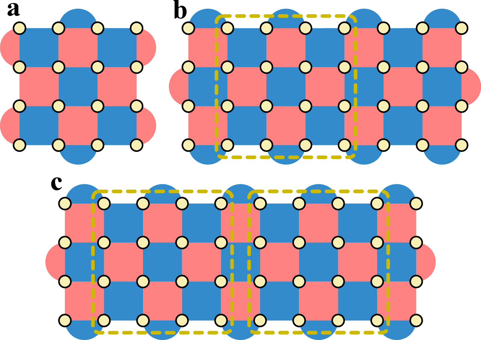
We now describe the level-0 implementation of an \(H\)-transformed readout gadget. The level-1 ancilla of the gadget is implemented by a shuttle bus, referred to as an \(H\) bus. In the first step, the \(H\) bus is transversally initialized in the \(Z\) basis as a \(Z\) bus. Then, the sequence of level-1 CNOT gates between level-1 data qubits (controls) and the level-1 ancilla (target) is implemented by core-bus CNOT gates between the corresponding cores and the \(H\) bus. In the third step, we apply a layer of transversal \(H\) gates on all data qubits of the \(H\) bus, thereby implementing a logical \(H\) gate on the level-1 ancilla and transforming the bus into an \(X\) bus. We group this layer of transversal \(H\) gates with the following level-0 SE round as a level-0 time step. Similarly, level-1 CNOT gates in the fourth step are implemented by bus-core CNOT gates between the \(H\) bus (control) and cores (targets). Finally, the \(H\) bus is transversally measured in the \(X\) basis. Similar to \(X\)-basis and \(Z\)-basis readout gadgets, we insert padding level-0 SE rounds on the \(H\) bus, so that (i) every two core-bus (or bus-core) CNOT gates in this gadget are separated by at least \(\alpha_{\mathsf{b}}\) level-0 SE rounds and (ii) transversal initialization and measurement are separated from the following and the preceding hybrid-unit CNOT gates, respectively, by at least \(\alpha_{\mathsf{b}}\) level-0 SE rounds. In addition, we require the layer of transversal \(H\) gates to be separated from any core-bus or bus-core CNOT gate by at least \(\alpha_{H}\) level-0 SE rounds. Here, \(\alpha_{H}\) is a new compilation parameter. For an even distance \(d_{0}\), since the core has asymmetrical \(X\) and \(Z\) boundaries (Fig. 4 (d)), the \(H\) bus after the transversal \(H\) gate is mismatched with cores along \(X\) boundaries (Fig. 17 (ab)). Therefore, now the \(H\) bus only supports bus-core CNOT gates with up to \(d_{1}-1\) cores at a time. This minor issue can be fixed by using an \(H\) bus of length \(d_{0}d_{1}+2\) (Fig. 17). For simplicity, we will not make such a modification to the bus length in what follows.
![Figure 18: Mid-cycle transversal S gate. (a) CNOT gate schedule for a level-0 SE circuit on the rotated surface code. The same schedule is applied to H buses (after the transversal H gate). (bd) Mid-cycle states after ancilla reset, the first layer of CNOT gates, and the second layer of CNOT gates, respectively, during a level-0 SE round (adapted from Refs. [25], [41]). The last state is also called a half-cycle state. (e) Fold-transversal S gate applied on the half-cycle state of an H bus with d_{0}=3 and d_{1}=2. (f) Fold-transversal S gate for an H bus with d_{0}=4 and d_{1}=2. Both H buses in (ef) have long logical X operators. Each mid-cycle fold-transversal gate in (ef) is embedded in a single level-0 SE round and implements a logical S gate on the H bus.](/article/2606.22594/figs/mid_cycle_s_gate.png "fig:")
If \(x\cdot z\) is odd, there are two ways to measure \(\mathsf{P}_{xz}\). First, we can use a logical \(Y\) state as a catalyst to convert the logical measurement task back to the case above, where \(x\cdot z\) is even [40]. Suppose we reserve a single logical qubit in an HLP to host a logical \(Y\) state and we would like to perform the logical Pauli measurement \(\mathsf{P}_{xz}\) supported on other logical qubits. Then, we can instead measure \(\mathsf{P}_{xz}\cdot \overline{\mathsf{Y}}\) using the \(H\)-transformed logical readout gadget; here, \(\overline{\mathsf{Y}}\) is the logical \(Y\) operator corresponding to the logical \(Y\) state. In this way, we effectively measure \(\mathsf{P}_{xz}\) while preserving the logical \(Y\) state, which can be reused to assist future logical Pauli measurements. Alternatively, we can construct another readout gadget, called an \(HS\)-transformed readout gadget, to directly measure \(\mathsf{P}_{xz}\) without using ancillary logical states. The \(HS\)-transformed readout gadget works as follows.
Same as steps 14 for the \(H\)-transformed readout gadget.
Perform a level-1 \(S\) gate on the ancilla.
Measure the ancilla in \(X\) basis.
The level-0 implementation of an \(HS\)-transformed readout gadget mostly follows from that of an \(H\)-transformed readout gadget. The only new step for the former is to perform a logical \(S\) gate on the \(H\) bus. Following the approach in Ref. [41], we can perform a mid-cycle fold-transversal \(S\) gate by leveraging the dynamics of the level-0 SE circuit on the bus [25], [41] (see Fig. 18). We require the mid-cycle transversal \(S\) gate to be separated from both the preceding bus-core CNOT gate and the final transversal \(X\)-basis measurement by at least \(\alpha_{\mathsf{b}}\) level-0 SE rounds.
We note that the level-0 implementation of both \(H\)-transformed and \(HS\)-transformed readout gadgets requires numerical benchmarking to optimize the number of padding level-0 SE rounds required between two adjacent logical operations on an \(H\) bus. We leave this to future work. In the remainder of this subsection, we theoretically analyze circuits with \(H\)-transformed readout gadgets (in addition to \(X\)-basis and \(Z\)-basis readout gadgets) under the phenomenological depolarizing noise model. We will extend Theorem 2 to prove that level-1 \(X\) (or \(Z\)) errors are almost uncorrelated even in the presence of \(H\)-transformed gadgets. Based on this result, we then formulate and analyze an LMS based on \(H\)-transformed gadgets to reliably measure a logical operator \(\mathsf{P}_{xz}\) with \(x\cdot z=0\). (The case \(x\cdot z=1\) can also be handled by such an LMS, given a logical \(Y\) state.)
Consider a level-0 circuit consisting of \(X\)-basis, \(Z\)-basis, and \(H\)-transformed readout gadgets, together with level-0 SE rounds on all working units. As described in Sec. 1.6, we partition level-0 detectors on cores and shuttle buses in \(X\)-basis and \(Z\)-basis readout gadgets into \(\mathcal{D}_{\mathsf{B}_{\lozenge}}\), \(\mathcal{D}_{\mathsf{C}}\), and \(\mathcal{D}_{\mathsf{B}_{\blacklozenge}}\) and primitive level-0 \(X\) and \(Z\) errors on these working units into \(\mathcal{E}_{\mathsf{B}_{\lozenge}}\), \(\mathcal{E}_{\mathsf{C}}\), and \(\mathcal{E}_{\mathsf{B}_{\blacklozenge}}\). Since an \(H\) bus behaves similarly to an \(X\) or \(Z\) bus, we likewise partition the level-0 detectors on \(H\) buses into \(\mathcal{D}_{\mathsf{B}_{\lozenge}}\) and \(\mathcal{D}_{\mathsf{B}_{\blacklozenge}}\), and the primitive level-0 \(X\) and \(Z\) errors on these buses into \(\mathcal{E}_{\mathsf{B}_{\lozenge}}\) and \(\mathcal{E}_{\mathsf{B}_{\blacklozenge}}\).
For an \(H\) bus \(\sigma\) in an \(H\)-transformed gadget, let \(t_{H}\) be the level-0 time step containing the transversal \(H\) gate on \(\sigma\). Construction of level-0 detectors on \(\sigma\) before (or after) time step \(t_{H}\) is the same as that on a \(Z\) bus (or an \(X\) bus). Every level-0 detector generated at time step \(t_{H}\) consists of the measurement result on a \(Z\) or \(X\) stabilizer in time step \(t_{H}-1\) and the measurement result on the corresponding \(X\) or \(Z\) stabilizer in time step \(t_{H}\). We refer to a level-0 detector on the bus as upstream (or downstream) if it is supported on \(X\) (or \(Z\)) stabilizer measurements before time step \(t_H\) and \(Z\) (or \(X\)) stabilizer measurements at or after time step \(t_{H}\). We refer to primitive qubit \(Z\) (or \(X\)) errors at or before time step \(t_{H}\), \(X\) (or \(Z\)) stabilizer measurement errors before time step \(t_{H}\), qubit \(X\) (or \(Z\)) errors after time step \(t_{H}\), and \(Z\) (or \(X\)) stabilizer measurement errors at or after time step \(t_{H}\) as upstream (or downstream) errors. Then, we add all upstream and downstream level-0 detectors on \(H\) buses to \(\mathcal{D}_{\mathsf{B}_{\lozenge}}\) and \(\mathcal{D}_{\mathsf{B}_{\blacklozenge}}\), respectively; we add all upstream and downstream level-0 errors on these buses to \(\mathcal{E}_{\mathsf{B}_{\lozenge}}\) and \(\mathcal{E}_{\mathsf{B}_{\blacklozenge}}\), respectively. We can then construct all three level-0 decoding graphs and perform level-0 decoding according to Sec. 1.6. Define the upstream (or downstream) decoding subgraph on an \(H\) bus \(\sigma\) as the subgraph of \(\mathcal{G}_{\mathsf{B}_{\lozenge}}\) (or \(\mathcal{G}_{\mathsf{B}_{\blacklozenge}}\)) induced by the set of all upstream (or downstream) level-0 detectors on \(\sigma\).
We define the \(Z\)-basis (or \(X\)-basis) separation of an \(H\)-transformed readout gadget from another readout gadget as the minimum separation between a core-bus (or bus-core) CNOT gate in the \(H\)-transformed gadget and a core-bus (or bus-core) CNOT gate in the other. Suppose we are interested in a subset \(\mathcal{M}\) of readout gadgets, such that (i) \(X\)-basis (or \(Z\)-basis) readout gadgets in \(\mathcal{M}\) are separated by at least \(d_{0}\) level-0 time steps, and (ii) the \(X\)-basis and \(Z\)-basis separations of each \(H\)-transformed readout gadget in \(\mathcal{M}\) from any other readout gadget in \(\mathcal{M}\) are at least \(d_{0}\) level-0 time steps. Following notations in Sec. 2, we let \(\mathcal{E}_{\mathsf{B}_{\blacktriangledown}}\) be the subcollection of all level-0 errors in \(\mathcal{E}_{\mathsf{B}_{\blacklozenge}}\) on buses in \(\mathcal{M}\).
Consider a general level-0 residual error configuration \(f\). We know that \(f|_{\mathsf{B}_{\lozenge}}:=f_X|_{\mathsf{B}_{\lozenge}}\cup f_{Z}|_{\mathsf{B}_{\lozenge}}\) is a collection of \(X\)-basis cycles on \(X\) buses, \(Z\)-basis cycles on \(Z\) buses, and cycles on the upstream decoding subgraphs on \(H\) buses. We restrict all cycles in \(f|_{\mathsf{B}_{\lozenge}}\) to have a weight smaller than \(d_{0}d_{1}\) as we did in Sec. 2.2. Then, every cross-membrane cycle in \(f|_{\mathsf{B}_{\lozenge}}\) on an \(H\) bus is either an \(X\)-basis or \(Z\)-basis cycle. Let \(f^{\circ}\) denote the collection of propagated simple walks (on cores) from cycles in \(f|_{\mathsf{B}_{\lozenge}}\); let \(f_X^{\circ}\) (or \(f_{Z}^{\circ}\)) denote the collection of propagated simple walks (on cores) from \(X\)-basis (or \(Z\)-basis) cycles in \(f|_{\mathsf{B}_{\lozenge}}\). Then, \(f^{\circ}=f_{X}^{\circ}\cup f_{Z}^{\circ}\). Following Sec. 2.2, \(f_{X}^{\circ}\cup f_{X}|_{\mathsf{C}}\) is a disjoint union of \(X\)-basis closed walks on cores, such that each closed walk consists of propagated simple walks in \(f_{X}^{\circ}\) and length-1 walks (primitive level-0 errors) in \(f_{X}|_{\mathsf{C}}\). Let \(f_{X}^{\bullet}\) denote the propagated simple walks on buses in \(\mathcal{M}\) from these closed walks; we similarly define \(f_{Z}^{\bullet}\) as the propagated simple walks on buses in \(\mathcal{M}\) from \(f_{Z}^{\circ}\cup f_{Z}|_{\mathsf{C}}\).
Restricted to \(X\) (or \(Z\)) buses, \(f_Z^{\bullet}\cup f_{Z}|_{\mathsf{B}_{\blacktriangledown}}\) (or \(f_{X}^{\bullet}\cup f_{X}|_{\mathsf{B}_{\blacktriangledown}}\)) is a disjoint union of \(Z\)-basis (or \(X\)-basis) closed walks, potentially triggering readout errors on \(X\)-basis (or \(Z\)-basis) readout gadgets. However, restricted to the downstream decoding subgraph of an \(H\) bus, a closed walk may contain both \(X\)-basis walks in \(f_{X}^{\bullet}\cup f_{X}|_{\mathsf{B}_{\blacktriangledown}}\) and \(Z\)-basis walks in \(f_{Z}^{\bullet}\cup f_{Z}|_{\mathsf{B}_{\blacktriangledown}}\). In other words, restricted to \(H\) buses, \(f_{X}^{\bullet}\cup f_{X}|_{\mathsf{B}_{\blacktriangledown}}\cup f_{Z}^{\bullet}\cup f_{Z}|_{\mathsf{B}_{\blacktriangledown}}\) is a disjoint union of closed walks on downstream decoding subgraphs. We will choose the compilation parameter \(\alpha_{H}\) sufficiently large that closed walks containing walks from both \(f_{Z}^{\bullet}\) and \(f_X|_{\mathsf{B}_{\blacktriangledown}}\), or from both \(f_X^{\bullet}\) and \(f_{Z}|_{\mathsf{B}_{\blacktriangledown}}\), are strongly suppressed.
We assign two level-1 error locations during the lifetime of an \(H\) bus: a level-1 \(X\) error location (before the transversal \(H\) gate) and a level-1 \(Z\) error location (after the transversal \(H\) gate). Both error locations trigger the same readout error on the corresponding \(H\)-transformed readout gadget. Similar to Def. 4, we define the receptive zones for both error locations.
Definition 5 (Receptive zones for level-1 error locations on an \(H\) bus). Consider an \(H\) bus \(\sigma\) assigned with two primitive level-1 errors \(\mathsf{e}_{\mathsf{X}}\) and \(\mathsf{e}_{\mathsf{Z}}\) corresponding to the \(X\) error location and the \(Z\) error location, respectively. The receptive zone for \(\mathsf{e}_{\mathsf{X}}\) is the collection of all level-0 \(X\) error locations satisfying at least one of the following conditions.
The error location corresponds to a downstream error on \(\sigma\).
The error location is on a CNOT membrane of a core induced by a core-bus CNOT gate \(\Lambda_{t}\), which acts on \(\sigma\) at level-0 time step \(t\).
The receptive zone for \(\mathsf{e}_{\mathsf{Z}}\) is the collection of all level-0 \(Z\) error locations satisfying at least one of the following conditions.
The error location corresponds to a downstream error on \(\sigma\).
The error location is on a CNOT membrane of a core induced by a bus-core CNOT gate \(\Lambda_t\), which acts on \(\sigma\) at level-0 time step \(t\).
We generalize the definition of downstream webs (Def. 3). Let \(\{l_{1},\cdots,l_u\}\) be the collection of disjoint closed walks such that their union is \(f_{X}^{\bullet}\cup f_{X}|_{\mathsf{B}_{\blacktriangledown}}\cup f_{Z}^{\bullet}\cup f_{Z}|_{\mathsf{B}_{\blacktriangledown}}\). Consider two \(X\)-basis closed walks \(\ell_{1}\) and \(\ell_{2}\) as subsets of \(f_X^{\circ}\cup f_{X}|_{\mathsf{C}}\) on cores. Let \(\ell_{1}^{\bullet}\) and \(\ell_{2}^{\bullet}\) be the collections of propagated simple walks from \(\ell_{1}\) and \(\ell_{2}\), respectively. We say \(\ell_1\) and \(\ell_2\) are linked if there is a propagated simple walk in \(\ell_1^{\bullet}\) and another propagated simple walk in \(\ell_{2}^{\bullet}\) that belong to the same closed walk in \(\{l_1,\cdots,l_u\}\). Consider a set \(w\) consisting of closed walks on cores and native walks in \(f_{X}|_{\mathsf{B}_{\blacktriangledown}}\cup f_{Z}|_{\mathsf{B}_{\blacktriangledown}}\), such that (i) \(w|_{\mathsf{C}}\subset f_X^{\circ}\cup f_{X}|_{\mathsf{C}}\), (ii) \(w|_{\mathsf{B}_{\blacktriangledown}}\subset f_X|_{\mathsf{B}_{\blacktriangledown}}\cup f_Z|_{\mathsf{B}_{\blacktriangledown}}\) and contains no native closed walk, and (iii) \(\partial_{\blacktriangledown}w=0\). We say \(w\) is a generalized downstream fault web if \(w|_{\mathsf{C}}\) is a linked cluster of closed walks on cores.
We now extend Lemma 8 to bound \(f\) under certain additional restrictions. We follow the notation in Sec. 2.2, where the section map \(\mathbb{S}_{f}\) is defined, and the subscript \(\epsilon\) for a general level-0 error configuration denotes its physical-error component.
Lemma 12 (Extension of Lemma 8). Consider the general level-0 residual error configuration \(f\). We require that, for any closed walk \(l_{h}\) (\(h\in\{1,\cdots,u\}\)) on a downstream decoding subgraph of an \(H\) bus, if \(l_h\cap f_{X}|_{\mathsf{B}_{\blacktriangledown}}\neq \emptyset\), then (i) \(l_{h}\cap(f_{Z}^{\bullet})=\emptyset\), and (ii) \(\mathbb{S}_{f}(l_{h}\cap f_{Z}|_{\mathsf{B}_{\blacktriangledown}})\cap \mathbb{S}_{f}(\tilde{\ell})=\emptyset\) for every cross-membrane cycle \(\tilde{\ell}\) in \(f_X|_{\mathsf{B}_{\lozenge}}\). We can explicitly construct a level-1 \(X\) error \(\mathsf{f_X}=\mathsf{e}_1+\mathsf{e}_2+\cdots+\mathsf{e}_{|\mathsf{f}|}\), where each \(\mathsf{e}_{i}\) is a distinct primitive level-1 \(X\) error, such that \(f\) induces a level-1 error configuration that contains \(\mathsf{f_X}\) as a subconfiguration. Moreover, we can find two general level-0 error configurations \(\lambda_f\subset\mu_f\subset f\) such that (i) \(\lambda_f=e_1+\cdots+e_{|\mathsf{f_X}|}\) with each \(e_{i}\) a distinct primitive level-0 error whose \(X\)-basis projection is in the receptive zone of \(\mathsf{e}_{i}\), (ii) each connected component of \(\mu_f\) (on the level-0 adjacency graph) contains at least one element in \(\lambda_f\), and (iii) the weight of physical errors in \(\mu_f\), \(|\mu_f\cap \epsilon|\), is lower bounded by \(\max(|\mu_f|/4,d_0|\mathsf{f_X}|/2)\).
Proof. For a lightning walk \(l_{h}\) in \(\{l_{1},\cdots,l_{u}\}\) on an \(H\) bus \(\sigma\), we let \(l_{h}\) induce the primitive level-1 \(X\) error on \(\sigma\) if \(l_{h}\cap (f_{X}^{\bullet}\cup f_{X}|_{\mathsf{B}_{\blacktriangledown}})\neq \emptyset\); otherwise, we let \(l_{h}\) induce the primitive level-1 \(Z\) error on \(\sigma\). The first requirement on \(f\) guarantees that we can find a set \(\{w_1,\cdots,w_o\}\) of generalized downstream webs and a set of native closed walks \(\{l_{b_1},\cdots,l_{b_v}\}\subset \{l_1,\cdots,l_u\}\), such that (i) these webs and closed walks are all mutually disjoint, (ii) their union contains \(f_X^{\circ}\cup f_{X}|_{\mathsf{C}}\cup f_X|_{\mathsf{B}_{\blacktriangledown}}\) and is contained in \(f_{X}^{\circ}\cup f_{X}|_{\mathsf{C}}\cup f_X|_{\mathsf{B}_{\blacktriangledown}}\cup f_{Z}|_{\mathsf{B}_{\blacktriangledown}}\), and (iii) each \(l_{b_i}\) (\(i\in\{1,\cdots,v\}\)) intersects with \(f_{X}^{\bullet}\cup f_{X}|_{\mathsf{B}_{\blacktriangledown}}\). Let \(g=\left(\bigcup_{i=1}^{o}w_i\right)\cup\left(\bigcup_{i=1}^{v}l_{b_i}\right)\). Following Lemma 7, we can construct a level-1 \(X\) error configuration \(\mathsf{f}_{\mathsf{X}}:=\mathsf{e}_{1}+\cdots+\mathsf{e}_{|\mathsf{f}_{\mathsf{X}}|}\), with each \(\mathsf{e}_{i}\) a distinct primitive level-1 \(X\) error, such that \(g\) induces \(\mathsf{f}_{\mathsf{X}}\). Furthermore, we can find two level-0 error configurations \(\lambda_{X}\) and \(\mu\) with \(\lambda_{X}\subset \mu\subset (f_X\cup f_{Z})\), such that (i) \(\lambda_{X}=e_{X,1}+\cdots+e_{X,|\mathsf{f}_{\mathrm{X}}|}\) with each \(e_{X,i}\) a distinct level-0 \(X\) error in the receptive zone of \(\mathsf{e}_{i}\), (ii) each connected component of \(\mu\) on the level-0 adjacency graph contains at least one element in \(\lambda_{X}\), (iii) \(\mu|_{\mathsf{B}_{\lozenge}}\subset f_{X}|_{\mathsf{B}_\lozenge}\), \(\mu|_{\mathsf{C}}\subset f_X|_{\mathsf{C}}\), and \(\mu|_{\mathsf{B}_{\blacktriangledown}}\subset g\cap (f_X|_{\mathsf{B}_{\blacktriangledown}}\cup f_Z|_{\mathsf{B}_{\blacktriangledown}})\), and (iv) \(|\mu\cap (f_{X,\epsilon}\cup f_{Z,\epsilon})|\geq \max(|\mu|/4,d_{0}|\mathsf{f}_{\mathsf{X}}|/2)\). The second requirement on \(f\) guarantees that \(\mathbb{S}_f(\mu\cap f_{X,\epsilon})\cap \mathbb{S}_f(\mu\cap f_{Z,\epsilon})=\emptyset\), indicating that \(|\mathbb{S}_f(\mu)\cap f_{\epsilon}|\geq \max(|\mathbb{S}_f(\mu)|/4,d_{0}|\mathsf{f}_{\mathsf{X}}|/2)\). We then prove the lemma by setting \(\lambda_{f}=\mathbb{S}_{f}(\lambda_{X})\) and \(\mu_{f}=\mathbb{S}_f(\mu)\). ◻
We now state and provide the following theorem, which extends Theorem 2 to incorporate \(H\)-transformed gadgets.
Corollary 1 (Extension of Theorem 2). Consider a level-0 circuit composed of level-0 SE rounds on cores and shuttle buses and X-basis, \(Z\)-basis, and \(H\)-transformed readout gadgets. Suppose we are only interested in the results of a subset \(\mathcal{M}_1\) of readout gadgets, such that (i) the separation between every two \(X\)-basis (or \(Z\)-basis) readout gadgets in \(\mathcal{M}_1\) is at least \(d_{0}\); (ii) the \(X\)-basis and \(Z\)-basis separations between an \(H\)-transformed gadget and other gadgets are at least \(d_{0}\). The compilation parameters \(\alpha_{\mathsf{c}}\), \(\alpha_{\mathsf{b}}\), and \(\alpha_{H}\) are set as \(1\), \(d_{1}\), and \(2d_{1}\), respectively. We follow the notation in Theorem 2. Then, under the phenomenological depolarizing noise model with a noise rate \(p<1/(4r\mathfrak{e})^{10}\), except for a rare event with a probability upper bounded by \(2\mathsf{v}_{\mathsf{b}}(p/p_{th}')^{d_{0}d_{1}/2}\), the induced level-1 \(X\) (or \(Z\)) errors are local stochastic, each with a level-1 error rate upper bounded by \(z_{\mathrm{max}}(p/p_{th})^{d_{0}/2}\). Here, \(p_{th}'=1/(2r\mathfrak{e})^{10}\).
Proof. The proof idea is to exclude enough rare events so that the remaining physical error configurations induce general residual error configurations that would always meet the requirements in Lemma 12. In this way, the proof of Theorem 2 works.
Similar to the proof of Theorem 2, we first exclude the event \(\mathcal{B}\) that a general level-0 residual error configuration induces an \(X\)-basis cycle on an \(X\) bus, a \(Z\)-basis cycle on a \(Z\) bus, or an upstream cycle on an \(H\) bus, of weight at least \(d_{0}d_{1}\). According to Theorem 2, \(P(\mathcal{B})\leq \mathrm{v}_{\mathsf{b}}(p/\sqrt{p_{th}})^{d_{0}d_1/2}\).
Consider a general level-0 residual error configuration \(f\) corresponding to a connected component on the level-0 adjacency graph. Following the notations in Lemma 12, we now analyze when \(f\) would violate the two requirements therein. Consider a closed walk \(l_h\in\{l_1,\cdots,l_{u}\}\) on an \(H\) bus \(\sigma\) with \(l_h\cap f_{X}|_{\mathsf{B}_{\blacktriangledown}}\neq \emptyset\). Among the (mutually disjoint) closed walks on cores formed by \(f^{\circ}\cup f_{X}|_{\mathsf{C}}\cup f_{Z}|_{\mathsf{C}}\), let \(\{\ell_{1},\cdots,\ell_{a}\}\) be the subcollection of all sources of simple walks in \(l_{h}\cap (f_{X}^{\bullet}\cup f_{Z}^{\bullet})\). Among the cross-membrane cycles in \(f_X|_{\mathsf{B}_{\lozenge}}\cup f_Z|_{\mathsf{B}_{\lozenge}}\), let \(\{\tilde{\ell}_1,\cdots,\tilde{\ell}_{r}\}\) be the subcollection of all sources of simple walks in \(\bigcup_{i=1}^{a}(\ell_i\cap f^{\circ})\), and let \(\{\tilde{\ell}_{r+1},\cdots,\tilde{\ell}_{r+s}\}\) be the subcollection of all cycles that act on qubits in the support of \(l_h\cap f_{Z}|_{\mathsf{B}_{\blacktriangledown}}\). Define \(\ell=\bigcup_{i=1}^{a} \ell_{i}\), \(\tilde{\ell}=\bigcup_{i=1}^{r}\tilde{\ell}_i\), and \(\tilde{\ell}'=\bigcup_{i=1}^{s}\tilde{\ell}_{r+i}\). Define \[\begin{align} \label{eq:32downward32pyramid} \mu=&\big[\left(l_h\cap(f_{X}|_{\mathsf{B}_{\blacktriangledown}}\cup f_{Z}|_{\mathsf{B}_{\blacktriangledown}})\right) \nonumber \\ &\cup \left(\ell\cap \left(f_X|_{\mathsf{C}}\cup f_Z|_{\mathsf{C}}\right)\right)\cup \tilde{\ell}\cup \tilde{\ell}'\big]. \end{align}\tag{9}\] By construction, \(\mu\subset f_{X}\cup f_{Z}\) is a connected cluster on the level-0 decoding graph.
By MWPM decoding, we have the following bounds on \(\tilde{\ell}\) and \(\tilde{\ell}'\). \[\begin{align} \label{eq:32cloud32cycles32of32the32downward32pyramid} |\tilde{\ell}|\leq& 2|\tilde{\ell}\cap (f_{X,\epsilon}|_{\mathsf{B}_{\lozenge}})| \nonumber\\ |\tilde{\ell}'|\leq& 2|\tilde{\ell}'\cap (f_{X,\epsilon}|_{\mathsf{B}_{\lozenge}})| \end{align}\tag{10}\] As the total weight of propagated simple walks from \(\tilde{\ell}\) is upper bounded by \(|\tilde{\ell}|/2\) (Lemma 4), we see that \[\begin{align} \label{eq:32core32cycle32in32the32downward32pyramid} |\ell\cap (f_X|_{\mathsf{C}}\cup f_{Z}|_{\mathsf{C}})|\leq& 2|\ell\cap(f_{X,\epsilon}|_{\mathsf{C}}\cup f_{Z,\epsilon}|_{\mathsf{C}})| + |\tilde{\ell}_{||}|/2 \nonumber\\ |\ell|\leq& 2|\ell\cap(f_{X,\epsilon}|_{\mathsf{C}}\cup f_{Z,\epsilon}|_{\mathsf{C}})| + |\tilde{\ell}_{||}| \end{align}\tag{11}\] As \(\ell\) may contain both lightning and cross-membrane walks, the total weight of propagated simple walks from \(\ell\) is upper bounded by \(|\ell|\). Then, we have \[\begin{align} \label{eq:32root32of32downward32pyramid} |l_h\cap (f_{X}|_{\mathsf{B}_{\blacktriangledown}}\cup f_{Z}|_{\mathsf{B}_{\blacktriangledown}})|\leq& 2|l_h\cap (f_{X,\epsilon}|_{\mathsf{B}_{\blacktriangledown}}\cup f_{Z,\epsilon}|_{\mathsf{B}_{\blacktriangledown}})| + |\ell| \end{align}\tag{12}\] Combining Eqs. 10 , 11 , and 12 , we have \[\begin{align} \label{eq:32bounds32on32downward32pyramid} |\mu|/5\leq& |\mu\cap (f_{X,\epsilon}\cup f_{Z,\epsilon})|\nonumber\\ |l_h\cap (f_X|_{\mathsf{B}_{\blacktriangledown}}\cup f_Z|_{\mathsf{B}_{\blacktriangledown}})|+|\tilde{\ell}'|\leq& 2|\mu\cap (f_{X,\epsilon}\cup f_{Z,\epsilon})| \end{align}\tag{13}\] If \(l_h\) does not satisfy the first requirement in Lemma 12, then \(l_h\cap f_{Z}^{\bullet}\neq \emptyset\), which implies \[\label{eq:32H32bus32cycle32intersect32w32z32membrane} 2d_{0}d_{1}\leq|l_{h,\perp}|\leq |l_{h}\cap (f_X|_{\mathsf{B}_{\blacktriangledown}}\cup f_Z|_{\mathsf{B}_{\blacktriangledown}})|.\tag{14}\] If \(l_h\) does not satisfy the second requirement in Lemma 12, then \[\label{eq:32H32bus32cycle32down32up32mix} 2d_{0}d_{1}\leq |l_{h,\perp}| + |\tilde{\ell}_{\perp}'|\leq |l_h\cap (f_X|_{\mathsf{B}_{\blacktriangledown}}\cup f_Z|_{\mathsf{B}_{\blacktriangledown}})|+|\tilde{\ell}'|.\tag{15}\] From Eq. 13 , we see that both Eq. 14 and Eq. 15 imply \[\label{eq:32physical32errors32in32a32downward32pyramid} d_{0}d_{1}\leq |\mu \cap (f_{X,\epsilon}\cup f_{Z,\epsilon})|.\tag{16}\] Let \(\mu_{f}=\mathbb{S}_{f}(\mu)\). Then, the weight of physical errors in \(\mu_f\) is lower bounded by \(|\mu\cap (f_{X,\epsilon}\cup f_{Z,\epsilon})|/2\). From Eq. 13 and Eq. 16 , we see that when \(f\) violates either requirement in Lemma 12, we can find a subconfiguration \(\mu_{f}\subset f\), such that (i) \(\mu_f\) is a connected cluster on the level-0 decoding graph, (ii) \(\mu_{f}\) contains at least one downstream level-0 error on an \(H\) bus, and (iii) the weight of physical errors in \(\mu_f\) is lower bounded by \(\max(|\mu_{f}|/10,d_{0}d_{1}/2)\).
Consider the event \(\mathcal{B}'\) that the induced general level-0 residual error configuration violates at least one requirement in Lemma 12. Then, following the proof of Lemma 9, we have \[\begin{align} P(\mathcal{B}')\leq \mathrm{v}_{\mathsf{b}}\left(p/p_{th}'\right)^{d_{0}d_{1}/2} \end{align}\] We note that the right-hand side of the above inequality also upper bounds \(P(\mathcal{B})\). After discarding both \(\mathcal{B}\) and \(\mathcal{B}'\) (with a joint probability upper bounded by \(2\mathrm{v}_{\mathsf{b}}\left(p/p_{th}'\right)^{d_{0}d_1/2}\)), all induced general level-0 residual error configurations satisfy Lemma 12. Therefore, the proof of Theorem 2 also holds and provides the same upper bound for the level-1 error rate. ◻
We note that we have not optimized for a larger threshold value in the above corollary. We only aimed to prove that for a small enough error rate \(p\), except for a rare event with probability \(\sim p^{-d_{0}d_1/2}\), the induced level-1 \(X\) (or \(Z\)) errors are effectively uncorrelated with a level-1 error rate \(\sim p^{-d_{0}/2}\). This result then aligns with Theorem 2.
We now construct an LMS, referred to as an \(H\)-LMS, from \(H\)-transformed logical readout gadgets to reliably measure a logical operator \(\mathsf{P}_{xz}\) with \(x\cdot z=0\). We note that the level-1 decoding process for a single \(H\)-LMS simultaneously involves level-1 \(X\) and \(Z\) errors. However, Corollary 1 only proves that the level-1 \(X\) (or \(Z\)) errors are almost uncorrelated but does not rule out correlation between level-1 \(X\) and \(Z\) errors. In practice, it is empirically observed that logical \(X\) and \(Z\) errors on an idling RSC are almost uncorrelated [1]. Thus, we may expect that we can effectively regard level-1 \(X\) and \(Z\) errors in an HLP as uncorrelated. Under this assumption, the \(H\)-LMS only requires \(d_{1}\) logical readout gadgets to achieve full level-1 distance. We note that future numerical benchmarking is required to substantiate this.
To guarantee the worst-case performance, we show in the following that an \(H\)-LMS, now consisting of \(4d_{1}\) logical readout gadgets across \(4d_1\) consecutive level-1 SE rounds, can reach similar logical performance even without the assumption above. We will use a modified level-1 decoding procedure (Algorithm 19). Based on this decoding procedure, we analyze the performance of this LMS without the above assumption.
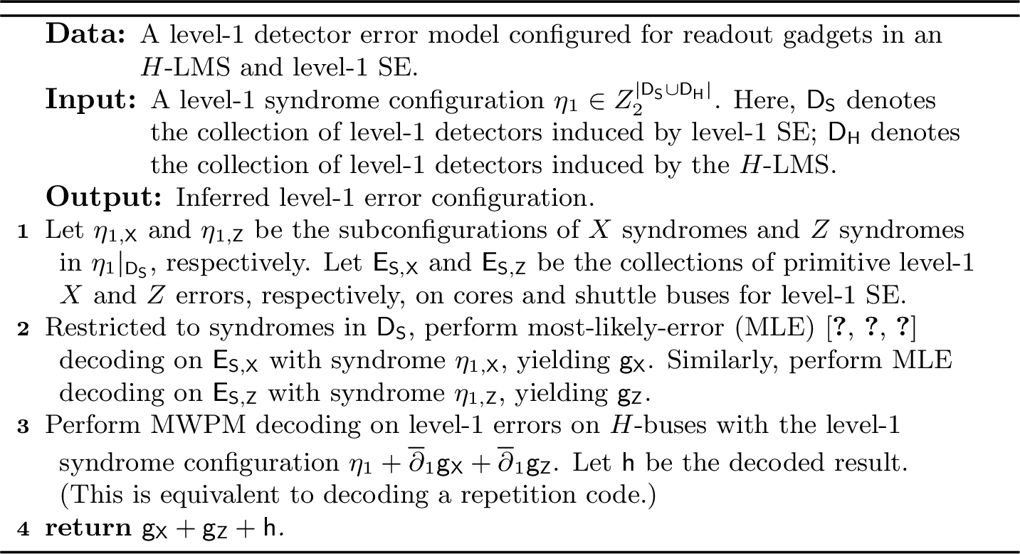
Corollary 2 (Fault probability for an \(H\)-LMS). Consider an HLP run for \(\mathsf{T}\) level-1 SE rounds with a collection of \(X\)-basis and \(Z\)-basis LMSs and \(H\)-LMSs. Every \(H\)-LMS uses \(4d_1\) \(H\)-transformed logical readout gadgets. We assume perfect time boundaries for the HLP. We focus on a fixed \(H\)-LMS executed on the HLP. We set compilation parameters \(\alpha_{\mathsf{c}}=1\), \(\alpha_{\mathsf{b}}=d_{1}\), and \(\alpha_{H}=2d_1\). We require that every \(H\)-transformed logical readout gadget is separated from all other logical gadgets in the same LMS, as well as from readout gadgets for level-1 SE, by at least \(d_{0}\) level-0 time steps in the \(X\)-basis and \(Z\)-basis separations. We follow the notation in Theorem 3. Then, under the phenomenological depolarizing noise model with an error rate \(p<1/(4r\mathfrak{e})^{10}\) at level 0 and with \(d_{0}\geq d_{H}\), the probability of a logical measurement error for the \(H\)-LMS is upper bounded by \(C_{H}(p/p_{th})^{d_{0}d_{1}/4}+2\mathrm{v}_{\mathsf{b}}(p/p_{th}')^{d_{0}d_{1}/2}\). Here, \(d_H=2\log\left((4r_H\mathfrak{e})^4z_{\mathrm{max}}\right)/\log(p_{th}/p)\), \(C_{H}=N_H\left((2r_H\mathfrak{e})^2\sqrt{z_{\mathrm{max}}}\right)^{d_1}\), \(N_H=(n(\delta_1+2)+s_1)\mathsf{T}+8d_1\), \(r_{H}=16\delta_1^2\max(\varpi_1,\varpi_L)\), and \(p_{th}'=1/(2r\mathfrak{e})^{10}\).
Proof. Throughout this proof, ‘\(H\) buses’ refers to \(H\)-buses in the \(H\)-LMS, and ‘logical measurement error’ refers to the logical measurement error for the \(H\)-LMS. Subscripts ‘\(\epsilon\)’ and ‘\(\kappa\)’ for a level-1 error configuration denote the induced-error component and the inferred-error component, respectively. We construct the level-1 error model and level-1 adjacency graph for \(H\) buses and buses for level-1 SE. Let \(\mathsf{D}_{\mathsf{S}}\) be the collection of level-1 detectors generated by level-1 SE. Similar to the proof of Theorem 3, each level-1 \(X\) or \(Z\) error triggers up to \(2\delta_{1}\) level-1 detectors. On the other hand, each level-1 detector can be triggered by up to \(2(\delta_1+1)\max(\varpi_1,\varpi_L)+4\leq 8\delta_{1}\max(\varpi_1,\varpi_L)\) primitive level-1 errors. Therefore, the vertex degree of each vertex in the level-1 adjacency graph is upper bounded by \(r_H=16\delta_1^2\max(\varpi_1,\varpi_L)\). Moreover, the number of level-1 errors is upper bounded by \(N_{H}=(n_1(\delta_1+2) +s_1)\mathsf{T}+8d_1\).
Consider a level-1 residual error configuration \(\mathsf{f}:=\mathsf{f}_{\mathsf{X}}+\mathsf{f}_{\mathsf{Z}}+\mathsf{h}\) obtained from Algorithm 19. Here, \(\mathsf{f}_{\mathsf{X}}\) and \(\mathsf{f}_{\mathsf{Z}}\) consist of level-1 \(X\) and \(Z\) errors, respectively, on cores and shuttle buses for level-1 SE; \(\mathsf{h}\) consists of level-1 errors on \(H\) buses. Without loss of generality, we assume \(\mathsf{f}\) is a connected cluster on the level-1 adjacency graph. Suppose \(\mathsf{f}\) results in a logical measurement error. If \(\mathsf{f}_{\mathsf{X}}\) (or \(\mathsf{f}_{\mathsf{Z}}\)) contains a weight-\(\mathrm{w}\) connected cluster with no syndrome in \(\mathsf{D}_{\mathsf{S}}\) and \(\mathrm{w}\geq d_{1}\), then this cluster contains at least \(\max(d_{1}/2,\mathrm{w}/2)\) induced level-1 \(X\) (or \(Z\)) errors. On the other hand, we now consider the opposite case that all weight-\(\mathrm{w}\) clusters in \(\mathsf{f}_{\mathsf{X}}\) or \(\mathsf{f}_{\mathsf{Z}}\) with no syndrome in \(\mathsf{D}_{\mathsf{S}}\) must satisfy \(\mathrm{w}<d_1\). According to Lemma 11, \(\mathsf{f}_{\mathsf{X}}\) (or \(\mathsf{f}_{\mathsf{Z}}\)) is equivalent to a level-1 error configuration \(\mathsf{h}_{\mathsf{X}}\) (or \(\mathsf{h}_{\mathsf{Z}}\)) consisting only of level-1 \(X\) (or \(Z\)) errors on \(H\) buses with \(|\mathsf{h}_{\mathsf{X}}|\leq |\mathsf{f}_{\mathsf{X}}|\) (or \(|\mathsf{h}_{\mathsf{Z}}|\leq|\mathsf{f}_{\mathsf{Z}}|\)). According to the MWPM decoding at the third step of Algorithm 19, we obtain \[|\mathsf{h}_{\kappa}|\leq |\mathsf{h}_{\epsilon}| + |\mathsf{h}_{\mathsf{X}}| +|\mathsf{h}_{\mathsf{Z}}|\] Moreover, as \(\mathsf{f}\) induces a logical measurement error, we have \[4d_1\leq |\mathsf{h}|+|\mathsf{h}_{\mathsf{X}}| + |\mathsf{h}_{\mathsf{Z}}|\] Note that \(|\mathsf{h}_{\mathsf{X}}|\leq |\mathsf{f}_{\mathsf{X}}|\leq 2|\mathsf{f}_{\mathsf{X},\epsilon}|\) and similarly, \(|\mathsf{h}_{\mathsf{Z}}|\leq 2|\mathsf{f}_{\mathsf{Z},\epsilon}|\). We can then bound the total weight of level-1 physical errors. \[\begin{align} d_1\leq& |\mathsf{h}_{\epsilon}|+|\mathsf{f}_{\mathsf{X},\epsilon}| + |\mathsf{f}_{\mathsf{Z},\epsilon}|=|\mathsf{f}_{\epsilon}|\nonumber\\ |\mathsf{f}|=&|\mathsf{h}|+|\mathsf{f}_{\mathsf{X}}|+|\mathsf{f}_{\mathsf{Z}}|\leq 4|\mathsf{f}_{\epsilon}| \end{align}\]
Let \(\mathfrak{E}\) be a set of all level-1 residual error configurations that (i) correspond to a connected cluster on the level-1 adjacency graph and (ii) contain at least \(\max(d_{1}/2,\mathrm{w}/4)\) level-1 \(X\) induced errors or at least \(\max(d_{1}/2,\mathrm{w}/4)\) level-1 \(Z\) induced errors with \(\mathrm{w}\) the weight of this cluster. Then, according to Lemma 10, the number of weight-\(\mathrm{w}\) elements in \(\mathfrak{E}\) is upper bounded by \(N_{H}(r_H\mathfrak{e})^{\mathrm{w}-1}\). According to our analysis above, the event of a logical measurement error is contained in the event of inducing a residual configuration in \(\mathfrak{E}\). We now discard the rare event in Corollary 1, so that the induced level-1 \(X\) (or \(Z\)) errors are uncorrelated with a level-1 error rate upper bounded by \(z_{\mathrm{max}}(p/p_{th})^{d_{0}/2}\). By Lemma 9, we upper bound the probability of inducing an element in \(\mathfrak{E}\) as follows. \[\begin{align} P(\mathfrak{E})\leq N_H((2r_H\mathfrak{e})^4p_1)^{d_1/2}, \end{align}\] where we used \(d\geq d_{H}\) to guarantee \(p_{1}\leq 1/(4r_H\mathfrak{e})^4\). Therefore, accounting for the discarded event, the probability for a logical measurement error is upper bounded by \(C_{H}(p/p_{th})^{d_{0}d_{1}/4} + 2\mathrm{v}_{\mathsf{b}}(p/p_{th}')^{d_{0}d_{1}/2}\). ◻
From the above corollary that upper bounds the probability of logical measurement error for a single \(H\)-LMS, we can follow Theorem 3 to bound the probability of logical measurement errors for multiple LMSs (possibly including \(X\)-basis LMSs, \(Z\)-basis LMSs, and \(H\)-LMSs) on an HLP. We omit the exact error bound computation for brevity.
3.3 Extension module II: interfacing with external cores↩︎
As shown in Fig. 3 (f), we can perform a transversal CNOT gate with an external core (a distance-\(d_{ext}\) RSC with \(d_{0}\leq d_{ext}\leq d_{0}d_{1}\)) as the control and a \(Z\) bus as the target. We call such a gate an extended core-bus CNOT gate. Similarly, we can perform an extended bus-core CNOT gate between an \(X\) bus and an external core. Equipped with these extended hybrid-unit CNOT gates, the previously developed readout gadgets can jointly measure logical qubits on an HLP and on external cores. Note that we only allow external cores to directly interact with shuttle buses but not internal cores, therefore errors on external cores do not propagate to internal cores. Consider a simple setting where external cores are only allowed to interact with an HLP via readout gadgets but not with other external cores. Then, level-0 circuits on external cores have the same structure as those on internal cores. In this way, we can apply the arguments in Sec. 2 and Sec. 3.2 to bound level-1 error rates and the probability of logical measurement errors for LMSs in the presence of external cores. By analogy with Theorem 2 and Corollary 1, we expect that (i) level-1 \(X\) (or \(Z\)) errors are still local stochastic, (ii) the level-1 error rate on internal cores and shuttle buses scales as \(\sim p^{d_{0}/2}\), and (iii) the level-1 error rate on external cores scales as \(\sim p^{d_{ext}/2}\). Similarly, by analogy with Theorem 3 and Corollary 2, we expect the probability of logical measurement errors to be upper bounded by both \(\sim p^{d_{ext}/2}\) and \(\sim p^{d_{0}d_{1}/4}\). More generally, consider a hybrid architecture consisting of HLPs and external cores. Each HLP can perform its own logical Clifford operations with previously introduced LMSs and simultaneously interface with a subcollection of external cores. External cores that are currently not interfacing with any HLP can prepare special logical states (such as magic states) and participate in transversal logical Clifford gates. In this way, HLPs and external cores can collaborate to execute logical quantum computation (Fig. 20). We leave a careful theoretical and numerical analysis of this hybrid architecture for future work.
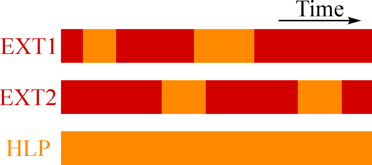
4 Numerical Simulation↩︎
In this section, we present concrete HLP designs and provide details of numerical simulations and performance extrapolation.
4.1 Details on HLP constructions and circuit-level simulation↩︎
![Figure 21: Level-1 SE circuit for the [[4,2,2]] Iceberg code. The level-1 Z and X stabilizers are extracted sequentially with one shuttle bus at a time.](/article/2606.22594/figs/iceberg_se.png "fig:")
As described in the main text, we can either use one shuttle bus at a time (Fig. 21) or two shuttle buses concurrently to implement the level-1 SE for an HLP based on the Iceberg code. For a \([[n^2,n-4n+2,4]]\) Square Berg code (\(n\) is divisible by 4) [1], we measure \(4n\) stabilizers in each level-1 SE round. As shown in Fig. 2 (a), among these stabilizers, there is one \(X\) stabilizer and one \(Z\) stabilizer associated with each row and each column. To perform a round of level-1 SE on an HLP based on a Square Berg code, we can use \(n\) shuttle buses at a time to measure the \(Z\) stabilizers of all columns, followed by \(X\) stabilizers of all columns, \(Z\) stabilizers of all rows, and finally \(X\) stabilizers of all rows. We use this level-1 SE design for the two HLPs based on the \([[64,34,4]]\) and \([[256,194,4]]\) Square Berg codes in Fig. 2.
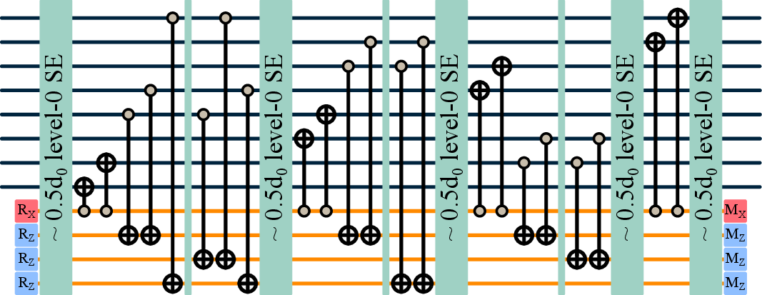
For simulating logical memories with perfect time boundaries, we follow the approach in Ref. [1] to simultaneously detect logical \(X\) and \(Z\) errors. More specifically, for every logical qubit, we associate it with a perfect physical qubit, referred to as the register qubit. For each logical qubit \(i\), let \(\overline{\mathsf{X}}_{i}\) and \(X_i\) denote the logical \(X\) operator and the Pauli \(X\) operator on the associated register qubit, respectively. Similarly, let \(\overline{\mathsf{Z}}_{i}\) and \(Z_i\) be the logical \(Z\) operator and the Pauli \(Z\) operator on the register qubit, respectively. To perfectly initialize the logical memory, we first measure all (level-0 and level-1) stabilizers perfectly, then we measure \(\overline{\mathsf{X}}_{i}\otimes X_{i}\) and \(\overline{\mathsf{Z}}_{i}\otimes Z_{i}\) perfectly for every logical qubit \(i\), thereby effectively creating a Bell pair between every logical qubit and its register qubit. After initialization, register qubits are left idling without noise, while qubits and gates in logical memory are subject to circuit-level noise. Finally, we repeat the perfect measurement procedure used in initialization. In this way, both logical \(X\) and \(Z\) errors can be detected simultaneously. If the logical qubit \(i\) is initialized or measured by measuring both \(\overline{\mathsf{X}}_i\otimes X_i\) and \(\overline{\mathsf{Z}}_i\otimes Z_i\), then we say this logical qubit is initialized or measured in the Bell basis. On the other hand, if a logical qubit \(i\) is initialized or measured by measuring \(\overline{\mathsf{X}}_i\) (or \(\overline{\mathsf{Z}}_i\)), then we say this logical qubit is initialized or measured in the \(X\) (or \(Z\)) basis.
In Fig. 3 (c), we present circuit-level simulations for benchmarking logical Pauli \(Z\) measurements (implemented with LMSs) on an HLP based on the \([[8,6,2]]\) Iceberg code with compilation parameters \(\alpha_{\mathsf{c}}=1\) and \(\alpha_{\mathsf{b}}=0.5\). We simulated three circuits, all having perfect time boundaries and running the HLP for five level-1 SE rounds, where the level-1 \(X\) and \(Z\) stabilizers are measured sequentially, as in Fig. 21. The first is a memory baseline circuit with six logical qubits initialized and measured in the Bell basis. Here, each logical qubit \(i\in\{1,\cdots 6\}\) is assigned a logical \(X\) operator \(\overline{\mathsf{X}}_i=\mathsf{X}_{1}\otimes \mathsf{X}_{i+1}\) and a logical \(Z\) operator \(\overline{\mathsf{Z}}_i=\mathsf{Z}_{i+1}\otimes \mathsf{Z}_{8}\). The second and the third circuits contain one and three LMSs, respectively. Since the LMS in the second circuit exactly corresponds to one LMS in the third circuit, we elaborate on the latter in the following. As described in the main text, the three LMSs measure three logical \(Z\) operators: \(\overline{\mathsf{Z}}_1\otimes\cdots \otimes\overline{\mathsf{Z}}_6\), \(\overline{\mathsf{Z}}_{1}\otimes \overline{\mathsf{Z}}_2 \otimes \overline{\mathsf{Z}}_3\), and \(\overline{\mathsf{Z}}_4\otimes \overline{\mathsf{Z}}_5\otimes\overline{\mathsf{Z}}_6\), respectively. We define a new set of logical qubits with the following logical \(X\) and \(Z\) operators. \[\begin{array}{ll} \overline{\mathsf{Z}}'_1:=\overline{\mathsf{Z}}_1\otimes\cdots\otimes \overline{\mathsf{Z}}_{6}, & \overline{\mathsf{X}}_1':=\overline{\mathsf{X}}_{6}\\ \overline{\mathsf{Z}}'_2:=\overline{\mathsf{Z}}_1\otimes\overline{\mathsf{Z}}_2\otimes \overline{\mathsf{Z}}_{3}, & \overline{\mathsf{X}}_2':=\overline{\mathsf{X}}_1\otimes\overline{\mathsf{X}}_{6}\\ \overline{\mathsf{Z}}'_3:=\overline{\mathsf{Z}}_2, & \overline{\mathsf{X}}_3':=\overline{\mathsf{X}}_1\otimes\overline{\mathsf{X}}_{2}\\ \overline{\mathsf{Z}}'_4:=\overline{\mathsf{Z}}_3, & \overline{\mathsf{X}}_4':=\overline{\mathsf{X}}_1\otimes\overline{\mathsf{X}}_{3}\\ \overline{\mathsf{Z}}'_5:=\overline{\mathsf{Z}}_4, & \overline{\mathsf{X}}_5':=\overline{\mathsf{X}}_4\otimes\overline{\mathsf{X}}_{6}\\ \overline{\mathsf{Z}}'_6:=\overline{\mathsf{Z}}_5, & \overline{\mathsf{X}}_6':=\overline{\mathsf{X}}_5\otimes\overline{\mathsf{X}}_{6} \end{array}\] We initialize and finally measure the first two logical qubits in the \(Z\) basis and the remaining logical qubits in the Bell basis, such that (i) the LMS outcomes are predetermined by initialization and (ii) errors on logical degrees of freedom not measured by the LMSs can be detected. The two logical readout gadgets in each LMS are embedded in the third and fourth level-1 SE rounds, respectively. More specifically, each logical readout gadget is contained within the lifetime of an \(X\) bus for measuring the level-1 \(X\) stabilizer. The scheduling of three logical readout gadgets corresponding to the three LMSs inside a single level-1 SE round is shown in Fig. 22. We note one anomaly in the scheduling: a core-bus CNOT gate coupling the \(Z\) bus on the bottom of Fig. 22 to two cores is now split into two adjacent level-0 time steps to avoid multiple core-bus CNOT gates operating on the same core at the same time. This scheduling choice does not comply with the restrictions imposed in Sec. 1. However, these restrictions are primarily introduced to simplify the analysis and presentation rather than to represent hard architectural constraints; practical implementations generally provide additional scheduling degrees of freedom beyond those assumed in our analysis. The simulation results presented in Fig. 3 (c) further validate this point.
As mentioned in Sec. 1.6, we use correlated level-0 decoding in our circuit-level simulations. We extract soft outputs at the end of this procedure. We note that correlated level-0 decoding reduces to correlated matching [68] for an idling core.
4.2 Soft-output Simulation↩︎
In this subsection, we describe a high-speed heuristic sampling method, soft-output simulation, that directly simulates a level-1 circuit by sampling level-1 errors and then performing level-1 decoding. This method is essentially the gap simulation method developed in Ref. [1] with gap values replaced by soft outputs [39]. The level-1 circuit error model we use is more refined than the one in Ref. [1].
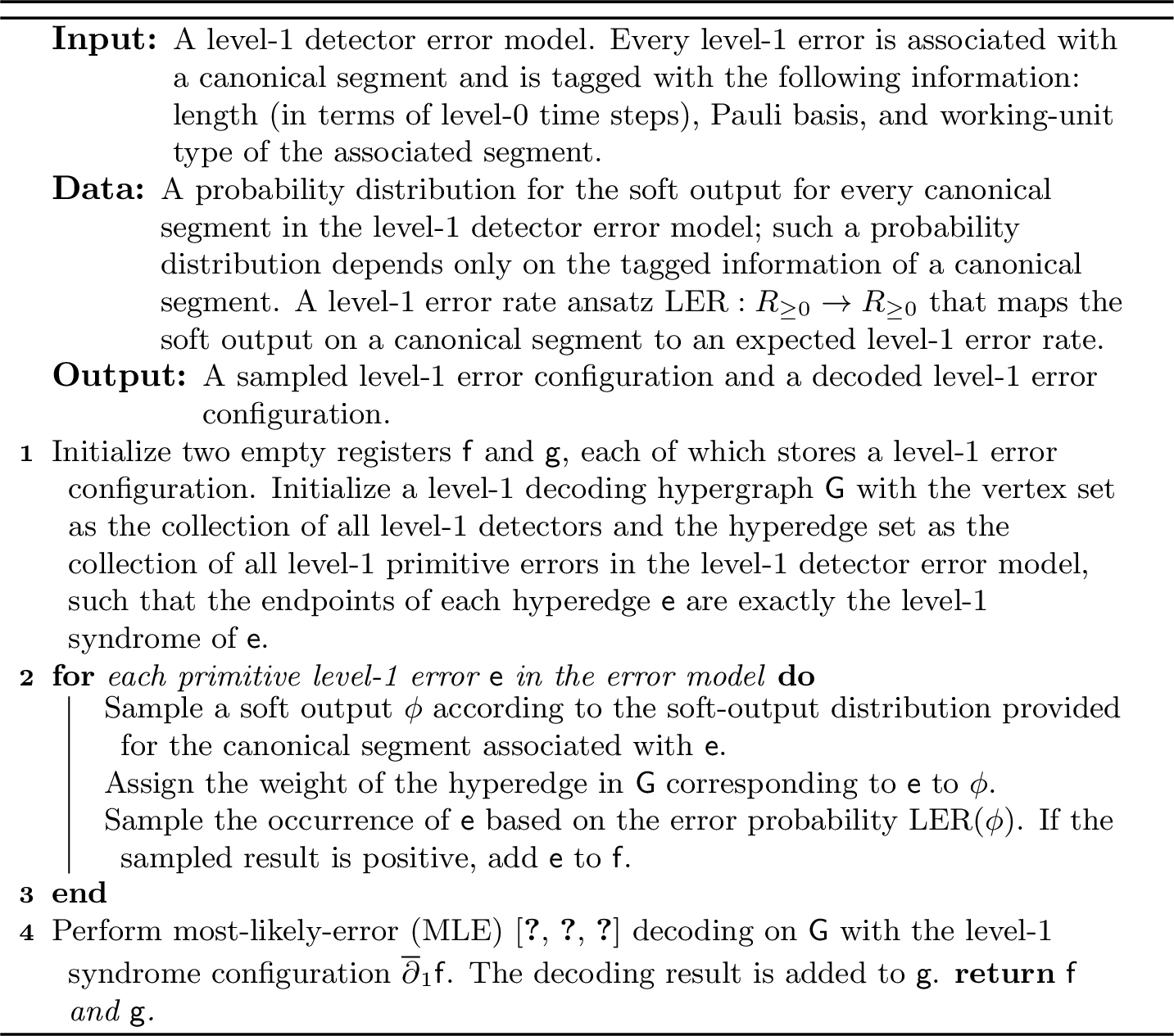
The soft-output simulation procedure is described in Algorithm 23, which requires two key ingredients. First, we need to efficiently construct the soft-output distribution for canonical segments with various lengths, Pauli basis, and working-unit types under different values of \(d_{0}\). Secondly, we need to construct the function \(\mathrm{LER}\) that infers the level-1 error probability for a canonical segment based on its soft output. We elaborate on these ingredients in the following.
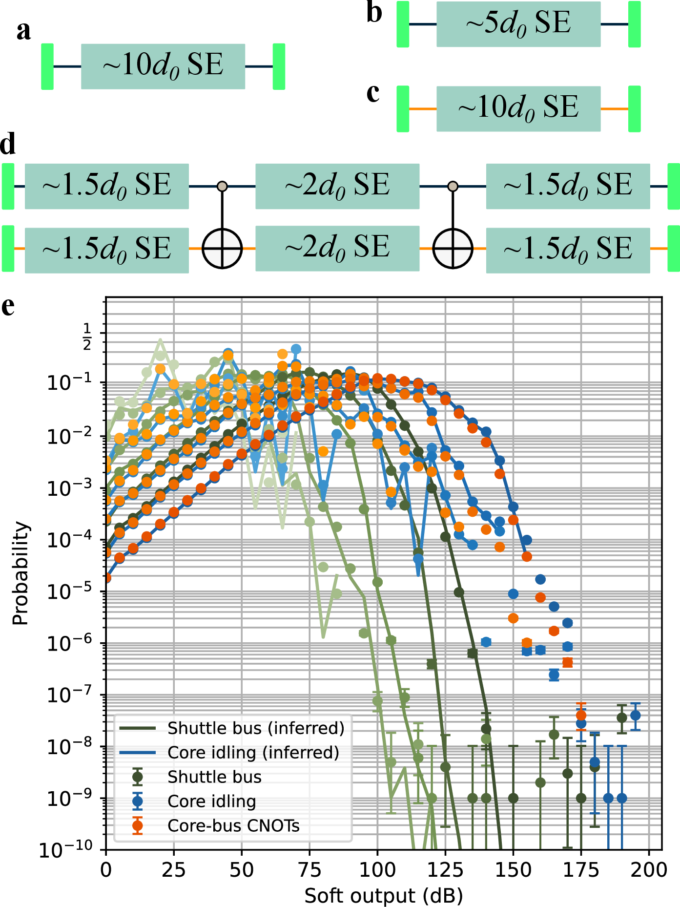
Soft-output distributionWe first construct a reference soft-output distribution on core segments with a fixed length of \(10d_{0}\) for each core size \(d_{0}\in\{3,4,\cdots,12\}\). To achieve this, we perform circuit-level simulation of an idling circuit on a single core with \(10d_{0}\) level-0 SE rounds (Fig. 24 (a)). For each simulation shot, we extract a pair of soft outputs [39], one on the \(X\)-basis and one on the \(Z\)-basis segment, where both segments span all level-0 SE rounds. From these reference distributions, we can heuristically infer soft-output distributions for canonical segments on cores and shuttle buses [1]. Denote the soft-output distribution on an \(X\)-basis (or \(Z\)-basis) core segment with a length of \(t\) level-0 time steps and a core size \(d_{0}\) as \(P_{X,t,d_0}\) (or \(P_{Z,t,d_{0}}\)). Define the corresponding complementary cumulative distribution function (CCDF) \(\overline{F}_{A,t,d_{0}}\) (\(A\in\{X,Z\}\)) by \(\overline{F}_{A,t,d_0}(\phi):=\sum_{\phi'\geq\phi}P_{A,t,d_{0}}(\phi')\). Following Ref. [1], from our reference CCDF \(\overline{F}_{A,10d_{0},d_{0}}\) (obtained from the reference distribution above), we heuristically infer another CCDF \(\overline{F}_{A,t',d_{0}}\) corresponding to a segment length \(t'\) as \[\label{eq:32CCDF32inference} \overline{F}_{A,t',d_{0}}(\phi):=\left(\overline{F}_{A,10d_{0},d_{0}}(\phi)\right)^{\frac{t'}{10d_{0}}}.\tag{17}\] As a CCDF uniquely determines a distribution, we can obtain from Eq. 17 the soft-output distribution \(P_{A,t',d_{0}}\). Similarly, consider an \(X\) (or \(Z\)) bus with a width of \(d_{0}\) and a length of \(d_{0}d_{1}\). Denote the soft-output distribution on an \(X\)-basis (or \(Z\)-basis) segment with a length of \(t\) as \(P_{A,t,d_{0},d_{1}}\) with \(A=X\) (or \(A=Z\)); denote the corresponding CCDF as \(\overline{F}_{A,t,d_{0},d_{1}}\), which is inferred as \[\overline{F}_{A,t,d_{0},d_{1}}(\phi) := \left(\overline{F}_{A,10d_{0},d_{0}}(\phi)\right)^{\frac{td_1}{10d_{0}}}.\] We test the validity of this heuristic inference method by comparing the inferred soft-output distributions with the numerically sampled ones for the circuits in Fig. 24 (bd) and observe close agreement between the two (Fig. 24 (e)).
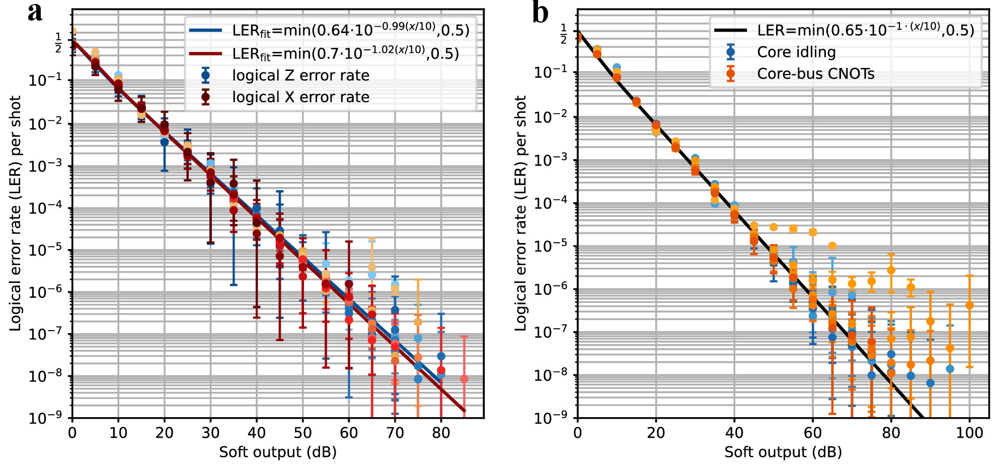
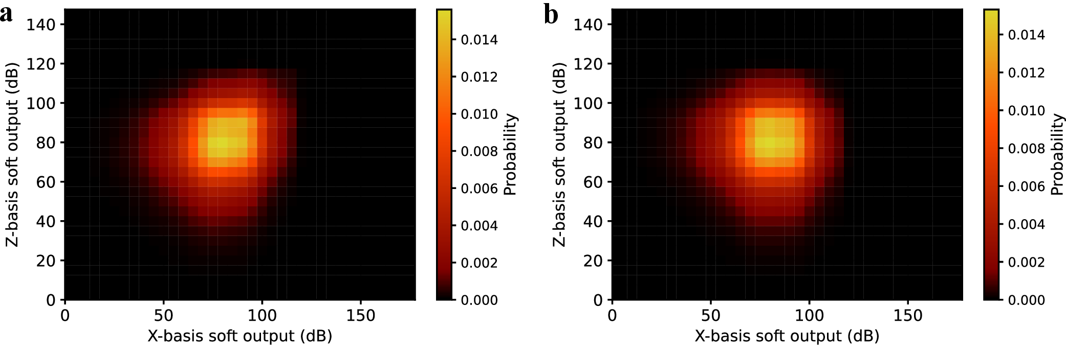
![Figure 27: Calibration of soft-output simulation. See also Fig. 2 (b) for an illustration of a subset of data points here. By default, compilation parameters \alpha_{\mathsf{c}} and \alpha_{\mathsf{b}} are both set to be 1. Additionally, we simulate the HLP based on the [[4,2,2]] Iceberg code at the circuit level with \alpha_{\mathsf{b}}=0.5.](/article/2606.22594/figs/memory_benchmark.png "fig:")
Level-1 error rate estimation from soft outputsWe use all sampling results for the core-idling circuit in Fig. 24 (a) with \(d_{0}\in\{3,\cdots,12\}\) to fit the following parametrized ansatz for estimating logical \(X\) (or \(Z\)) error rates from \(Z\)-basis (or \(X\)-basis) soft outputs: \[\label{eq:32ler32ansatz32for32soft32outputs} \mathrm{LER}_{a,b}(\phi):=\min(a\cdot 10^{-b\cdot\phi/10},0.5),\tag{18}\] where \(a\) and \(b\) are non-negative fitting parameters. We find that \(a=0.65\) and \(b=1\) provides a close fit for both logical \(X\) and \(Z\) error rates (Fig. 25 (a)). We compare this fitted ansatz with data pairs consisting of \(X\)-basis soft outputs and logical \(Z\) error rates on a core for circuits in Fig. 24 (b) and Fig. 24 (d). The fitted ansatz matches the data points well for the idling circuit in Fig. 24 (b), while data points for the circuit in Fig. 24 (d) containing core-bus CNOT gates exhibit some deviation at large soft output values for small \(d_{0}\)more specifically, logical \(Z\) error rates plateau at large soft output values. We attribute the deviation, at least in part, to logical \(Z\) errors on the \(Z\) bus between the two core-bus CNOT gates.
![Figure 28: Extrapolation of logical error rates per level-0 SE round for the rotated surface code (RSC) and hierarchical logical processors (HLPs). (a) Logical error rates of an idling RSC with distances ranging from 3 to 10. Data points are obtained from circuit-level simulations with a correlated-matching decoder [68]. (b) Logical error rates of HLPs based on Iceberg codes with one or two shuttle buses operating concurrently. (c) Logical error rates of HLPs based on the [[256,194,4]] Square Berg code with different limits on the number of concurrently operating shuttle buses during level-1 SE. Data points in (bc) are obtained from soft-output simulations. To account for the gap between the soft-output and the circuit-level results observed in Fig. 27, we multiply the soft-output logical error rates by a factor of two when estimating the logical error rates of HLPs. For the HLPs, logical error rates are fitted per level-1 SE round and converted to logical error rates per logical qubit per level-0 SE round for plotting.](/article/2606.22594/figs/hlp_extrapolation.png "fig:")
Soft outputs collected for the idling core (Fig. 24 (a)) also allow a fine-grained study of correlations between logical \(X\) and \(Z\) errors on the core. From these data, we obtain, for each core distance \(d_{0}\in\{3,\cdots,12\}\), both the joint distribution of \(X\)-basis and \(Z\)-basis soft outputs and the product of their marginal distributions. We observe close agreement between the joint distribution and the product distribution for all \(d_{0}\in\{4,\cdots,12\}\), indicating that the \(X\)-basis and \(Z\)-basis soft outputs are approximately independent. See Fig. 26 (ab) for an illustration of the \(d_{0}=7\) case. Since the \(X\)-basis and \(Z\)-basis soft outputs accurately predict probabilities for logical \(Z\) and \(X\) errors, respectively, this independence suggests that the logical error probability in one basis is insensitive to the component of physical-error configuration in the other basis, at the resolution captured by soft outputs. More specifically, we group physical-error configurations according to the \(Z\)-basis soft outputs determined by the \(X\)-basis components of those configurations. Across these groups, the logical \(Z\) error probability remains approximately unchanged. Conversely, we group physical-error configurations according to the \(X\)-basis soft outputs determined by the \(Z\)-basis components of those configurations. Across these groups, the logical \(X\) error probability remains approximately unchanged. Ref. [1] observed that the overall logical \(X\) and \(Z\) errors are approximately uncorrelated on an idling core. The fine-grained study above extends this observation to soft-output-conditioned logical error probabilities. As discussed in Sec. 3.2, if level-1 \(X\) and \(Z\) errors are uncorrelated, we expect an \(H\)-LMS with \(d_1\) \(H\)-transformed logical readout gadgets to achieve full level-1 distance. Without this assumption, Corollary 2 provides a worst-case guarantee for an \(H\)-LMS with \(4d_1\) such gadgets. The observation that level-1 \(X\) and \(Z\) errors on an idling core are approximately uncorrelated provides a starting point for future studies of correlations among level-1 \(X\) and \(Z\) errors on an HLP, as well as the optimization of \(H\)-transformed readout gadgets and \(H\)-LMSs.
As described in the main text (Fig. 2 (b)), we test the accuracy of soft-output simulation on the following two HLPs:
An HLP with the \([[4,2,2]]\) Iceberg code as the level-1 code. The HLP is run as a memory for ten level-1 SE rounds.
An HLP with the \([[64,34,4]]\) Square Berg code as the level-1 code. We simulate only five level-1 SE rounds on the HLP, since circuit-level simulation is costly at this scale.
As shown in Fig. 27, the soft-output simulations using the fitted level-1 error rate ansatz \(\mathrm{LER}_{0.65,1}\) produce results close to those obtained from circuit-level simulations. However, they consistently underestimate the logical error rates, and the gap grows slightly with increasing core distance \(d_{0}\). To reduce this dependence on \(d_{0}\), we use a slightly tuned ansatz \(\mathrm{LER}_{0.5,0.9}\), which yields slightly higher estimates of level-1 error rates than \(\mathrm{LER}_{0.65,1}\) at large soft-output values. With this ansatz, the gap between the soft-output and circuit-level simulations remains almost constant for both HLPs as \(d_{0}\) increases. We therefore use \(\mathrm{LER}_{0.5,0.9}\) for the soft-output simulations of the other HLPs in the following subsection. Moreover, to account for the remaining gap, we multiply the logical error rates obtained from the soft-output simulations by a factor of two when estimating the logical error rates of HLPs.
4.3 Extrapolation for logical error rates↩︎
In this subsection, we describe how we extrapolate the performance of the RSC and HLPs to obtain the qubit and time overhead estimation in Fig. 2 (cd). For the RSC, we perform circuit-level simulation of the idling circuit in Fig. 24 (a) with a correlated-matching decoder [68] and distance \(d_{0}\) ranging from \(3\) to \(10\). We fit the logical error rates (per SE round) as a function of the code distance to \(\mathrm{LER}_{\mathrm{RSC}}^{a,b}(d_{0})=a^{-d_{0}}/b\) (Fig. 28 (a)). For HLPs based on \([[n_1,n_1-2,2]]\) Iceberg codes with a single shuttle bus operating at a time, we use soft-output simulation (of \(10\) level-1 SE rounds) to estimate their logical error rates for code sizes \(n_1\in\{4,8,12\}\) and core distance \(d_{0}\) ranging from \(3\) to \(7\) (Fig. 28 (b)). Using data with \(d_{0}\in\{5,6,7\}\), we fit the logical error rates per level-1 SE round to \(\mathrm{LER}_{\mathrm{ICE}}^{a,b,c}(d_{0},n_1,r)=r^{c}\cdot n_1^2\cdot a^{-d_{0}}/b\), where \(r\) is the length of each level-1 SE round [1]. We expect the fitted parameter \(c\) to be close to the Iceberg-code distance [1]. Similarly, we use soft-output simulation to study HLPs based on Iceberg codes with two shuttle buses operating concurrently, and perform the same procedure described above (Fig. 28 (b)). For HLPs based on the \([[256,194,4]]\) Square Berg code with different numbers of concurrent shuttle buses, we perform soft-output simulation of 10 level-1 SE rounds and use the data with \(d_{0}\in\{5,6,7\}\) to fit the logical error rates per level-1 SE round to \(\mathrm{LER}_{\mathrm{SQR}}^{a,b,c}(d_{0},r)=r^{c}\cdot a^{-d_{0}}/b\) (Fig. 28 (c)). Based on these fitted logical error rate ansatzes, we can determine the core distance \(d_{0}\) required to attain a target logical error rate. This then allows us to estimate the qubit overhead per logical qubit and time overhead per level-1 SE round.