1 Introduction↩︎

Early work on nonlocal equations can be traced back to a study by Liouville in 1837 (cf. [1]), who investigated a parabolic equation with a nonlocal term depending on an integral of the unknown solution. The corresponding stationary solution also satisfies a nonlocal elliptic equation. Since then, the study of nonlocal elliptic equations has evolved significantly. These models are fundamental in many fields of science, as they often arise as stationary solutions of evolution equations with long-range interactions or spatial averaging, and appear in applications ranging from physics and electrochemistry to population dynamics and material systems with memory [2]–[9]. The diverse nature of these applications has motivated a rich body of research on the uniqueness, multiplicity and qualitative properties of solutions to such equations. Nevertheless, to the best of our knowledge, these topics in recent related works are not yet fully settled, even for linear elliptic equations with nonlocal terms.

This paper aims to contribute to the understanding of these topics by investigating a class of linear elliptic equations involving nonlocal nonlinearities in a bounded smooth domain \(\Omega \subset \mathbb{R}^m\) with \(m \geq 1\). We begin by introducing the following equation with a single nonlocal term \(\boldsymbol{\mathsf{N}}[\,\cdot\,]\) and positive parameters \(\lambda\) and \(\eta\): \[\label{eq-u} -\nabla\cdot(\mathsf{D}(x)\nabla u) +\lambda f(x)u= \eta h(x)\boldsymbol{\mathsf{N}}[u] \quad\text{in}\,\,\Omega,\tag{1}\] subject to the Robin boundary condition \[\label{rbd} u+b(x) \frac{\partial u}{\partial{\vec{\nu}}} = g(x)\quad\text{on}\,\,\partial\Omega.\tag{2}\] Equation 1 can be viewed as a linear inhomogeneous equation with a nonlocal coefficient. The solution \(u=u_{\lambda,\eta}\) depends on \(\lambda\) and \(\eta\), but we omit the subscript for simplicity. Here, \(\nabla\) and \(\nabla\cdot\) denote the gradient and divergence operators in \(\mathbb{R}^m\), respectively. \(\vec{\nu}\) is the unit outward normal vector to \(\partial\Omega\). The matrix-valued function \(\mathsf{D}= \left(D_{ij}\right)_{m\times m}\) defined on \(\overline{\Omega}\) is symmetric and satisfies a uniform ellipticity condition, with each entry \(D_{ij} \in\mathrm{C}^1( \overline{\Omega}; \mathbb{R})\). In Sections 2.1 and 2.2, we first provide a thorough argument to establish the existence of multiple solutions to a special form of 1 –2 .

We are particularly interested in elliptic equations with multiple nonlocal nonlinearities, as they are crucial for modeling systems where the steady-state behavior is not determined by local information alone, and the influencing factors are related through complex nonlinear relationships. In plasma physics, a single particle’s behavior is influenced not only by its immediate surroundings but also by the overall charge distribution throughout the plasma. This is a classic example of a nonlocal effect. When simultaneously considering the complex nonlinear interactions between multiple species, such as electrons and ions, the resulting equations contain multiple nonlocal nonlinear terms. For a more detailed look, the reader can refer to the papers mentioned in the first paragraph and the references therein.

Based on the insights from Sections 2.1–2.2, we extend our study to the more general equation \(-\nabla\cdot(\mathsf{D}(x)\nabla u) +\lambda f(x)u= \eta \sum_{j=1}^kh_j(x)\boldsymbol{\mathsf{N}}_j[u]+h_0(x)\) (cf. 15 ) with \(k\) multiple nonlocal terms (\(k\geq1\)). This investigation and its main results are detailed in Section 2.3.

1.1 Setting of the problem↩︎

Nonlocal elliptic equations inherently present challenges for rigorous mathematical analysis. A key difficulty is that the maximum principle generally fails in the presence of a nonlocal term in 1 , in contrast to some local-type elliptic equations where the maximum principle holds under appropriate assumptions [10]. To gain insight into the nonlocal effect, we assume that the local part of 1 satisfies the maximum principle. This allows us to proceed with the following assumptions on the coefficients \(\mathsf{D}=\left(D_{ij}\right)_{\color{black}{m\times m}}\), \(f\), \(h\), \(b\) and \(g\): \[\label{dhb} \begin{cases} \text{\boldsymbol{(}a).}\,\,(\text{uniform\,\, ellipticity})\,\, D_{ij}\in\text{C}^{1}(\overline{\Omega};\mathbb{R}),\,\,D_{ij}(x)=D_{ji}(x), \\ \sum\limits_{i,j=1}^mD_{ij}(x)z_iz_j\geq\mathfrak{D}|z|^2,\,\,{\forall}x\in\overline{\Omega}\,\,\text{and}\,\,z=(z_1,...,z_m)\in\mathbb{R}^m,\\ \text{where}\,\, \mathfrak{D}\,\, \text{is\, a\, positive\, constant};\\ \text{\boldsymbol{(}b).}\,\,f\in\text{C}^{0}(\overline{\Omega};(0,\infty)),\,\,\,h\in\text{C}^{0}(\overline{\Omega};\mathbb{R})\,\,\text{with}\,\,h\not\equiv0,\\ b\in\text{C}^{0}(\partial\Omega;[0,\infty))\,\,\text{and}\,\,g\in\text{C}^{0}(\partial\Omega;\mathbb{R}). \end{cases}\tag{3}\]

Equation 1 is a type of elliptic functional differential equations (cf. [11]). In particular, equation 1 becomes an integro-differential equation when the nonlocal term \(\boldsymbol{\mathsf{N}}[u]\) is represented by an integral involving the unknown solution \(u\) [12], [13]. This type of coupling often leads to qualitative behavior that differs significantly from the purely local case. Inspired by the study of integro-differential equations, particularly those of Fredholm type [14], [15], we specifically focus on two distinct types for the nonlocal term \(\boldsymbol{\mathsf{N}}[u]\): \[\label{N-2t} \boldsymbol{\mathsf{N}}[u]= \begin{cases} \displaystyle\int_\Omega w(y)\mathcal{N}(u(y))\,\mathrm{d}y&(\text{type~I}); \\ \displaystyle\mathcal{N}(\int_\Omega w(y)u(y)\,\mathrm{d}y)\qquad&(\text{type~II}), \end{cases}\tag{4}\] where \(w\) satisfies \(\int_\Omega w(y)\,\mathrm{d}y\neq0\). These two types of nonlocal terms are of particular interest as they introduce global dependencies into equation 1 . Their fundamental structural differences lead to a wide range of applications. For instance, a case related to the Type I nonlocal term in 4 was studied by Allegretto and Barabanova [16], specifically for nonlocal equations with separable kernels of the form \(h(x)\int_{\Omega}w(y)u(y)\,\text{d}y\). In particular, the assumption that \(\int_\Omega w(y)\,\mathrm{d}y\neq0\) is crucial to guarantee a non-trivial nonlocal effect. The setting in 4 also includes special cases of the average integral, such as \[\frac{1}{|\Omega|}\int_\Omega\mathcal{N}(u(y))\,\mathrm{d}y\quad\text{and}\quad\mathcal{N}\left(\frac{1}{|\Omega|}\int_{\Omega}u(y)\,\mathrm{d}y\right),\] where \(|\Omega|\) is the usual Lebesgue measure of \(\Omega\) in \(\mathbb{R}^m\). For the subsequent analysis, we require the following assumptions on the functions defined in 4 :

• \(\mathcal{N}:\mathbb{R}\to\mathbb{R}\) is locally Lipschitz continuous.

• The weight function \(w\in\mathrm{L}^p(\Omega)\) for some \(p>1\) and its values on \(\Omega\) are not restricted to a single sign. Without loss of generality, we normalize \(w\) by setting \(\int_\Omega w(y)\,\mathrm{d}y=1\).

It is worth noting that for some special cases, e.g., when \(f\equiv h\) and \(\lambda\neq\eta\), equation 1 –2 can be transformed into a linear elliptic equation with an integral type Robin boundary condition [17]. Specifically, if we further assume \(\mathcal{N}(s)=s\), one can define an auxiliary function \(U=u-\frac{\eta}{\lambda}\boldsymbol{\mathsf{N}}[u]\). We then obtain \(\boldsymbol{\mathsf{N}}[U]=(1-\frac{\eta}{\lambda})\boldsymbol{\mathsf{N}}[u]\) such that \(U\) satisfies the equation \(-\nabla\cdot(\mathsf{D}(x)\nabla U) +\lambda f(x)U=0\), in \(\Omega\), with the nonlocal boundary condition \(U+b(x) \frac{\partial U}{\partial{\vec{\nu}}} = g(x)+\frac{\eta{\eta-\lambda}}{\boldsymbol{\mathsf{N}}}[U]\) on \(\partial\Omega\). The similar argument can also be found in [18]–[21]. However, our focus in this paper is on a more general problem, and we will not pursue this specific transformation here.

1.2 Equations without variational structure↩︎

When the positive parameter \(\eta\) vanishes, 1 is reduced to a linear elliptic equation, which serves as a classical reference case. However, the nonlocal nature of the terms present in 4 generally means that equation 1 –2 does not have a variational structure. This poses a significant challenge for the use of standard classical tools from the calculus of variations, such as the direct method. Consequently, a different approach is necessary to establish the existence and multiplicity of solutions. In this paper, we overcome this challenge by developing a novel approach that combines fixed-point arguments with asymptotic techniques, which allows us to directly study the non-variational problem.

While the existence of multiple solutions for semilinear elliptic equations has been extensively studied using variational or topological methods, relatively fewer results are available when nonlocal terms are present. In particular, the influence of nonlocality on the multiplicity structure of solutions remains an open and interesting question in many settings. The aim of this paper is to understand under what conditions nonlocal effects may lead to the existence of multiple steady states, and how the structure of the nonlocal coupling influences this phenomenon.

Note that the nonlocal term \(\boldsymbol{\mathsf{N}}[u]\) in 1 can be viewed as a parameter-like coefficient that depends on the unknown solution \(u\). If we replace \(\boldsymbol{\mathsf{N}}[u]\) with any given constant, the resulting linear elliptic problem with the boundary condition 2 admits a unique solution due to the positivity of \(f\) and nonnegativity of \(b\). A fundamental problem is to determine the conditions under which equation 1 –2 admits a unique solution or multiple solutions. The main goal of this work can be summarized into the following two questions (Q1) and (Q2):

• Under what conditions on \(\lambda\) and \(\eta\) does the equation admit a unique solution?

• Under what conditions on \(\lambda\) and \(\eta\) does the equation admit multiple solutions? In this case, does the nature of the nonlocal term \(\boldsymbol{\mathsf{N}}[u]\) play a significant role in determining the number of solutions?

We assume that \(\mathcal{N}:\mathbb{R}\to\mathbb{R}\) is globally Lipschitz continuous to address question (Q1) from a theoretical standpoint. Specifically, we show that the solution to 1 –2 is unique provided that \(\frac{\eta}{\lambda}\) is sufficiently small. This elementary result is stated as follows.

Although the proof of Proposition 1 is based on the standard contraction mapping theorem, to the best of our knowledge, a similar result is not available in the literature. Therefore, a detailed proof is provided in Section 3 for the reader’s convenience.

The existence and uniqueness of a solution to equation 1 –2 is guaranteed by Proposition 1 when \(\mathcal{N}:\mathbb{R}\to\mathbb{R}\) is globally Lipschitz continuous and the parameter condition ?? is satisfied. Although this approach provides a solid foundation, the global Lipschitz assumption is a restrictive condition for many applications, and we observe that a unique solution may still exist even when conditions ?? or ?? are not met. In our previous work [14], we investigate the uniqueness and asymptotic behavior of solutions for a class of singularly perturbed linear Fredholm integro-differential equations. However, to date, to the best of our knowledge, we have only been able to obtain sufficient conditions for the uniqueness of solutions.

A more challenging and interesting problem is considered when \(\mathcal{N}:\mathbb{R}\to\mathbb{R}\) fails to satisfy global Lipschitz continuity. Such a situation often gives rise to various types of solution, including the possibility of multiple solutions. Therefore, we turn our attention to the assumption (A1) for \(\mathcal{N}:\mathbb{R}\to\mathbb{R}\). (Note that (A1) still includes the global case.) We will focus on the question (Q2), and develop a new approach to investigate the existence of multiple solutions and explore the rich solution structures that can emerge.

The plan of this paper↩︎

The remainder of this paper is organized as follows. Section 2 includes three subsections that present our proposed methodology and main results. More precisely, in Sections 2.1–2.2, we investigate equation 1 –2 with \(f=h\). We clearly demonstrate how multiple solutions can arise for this type of nonlocal equation by providing a specific framework that connects the nonlocal nonlinear term to the existence of multiple solutions. Based on this, we proceed in Section 2.3 to consider the general case with multiple nonlocal nonlinear terms, concluding with a statement of our main results: Proposition 2, Theorem 3, and Theorem 4. Section 3 contains the proof of Proposition 1. The proofs of Proposition 2 and Theorem 3 are given in Section 4, while the proof of Theorem 4 is provided in Section 5. Section 6 provides the concluding remarks of this work and discusses an outlook for our future research. Finally, the Appendix provides illustrative examples that demonstrate the validity of assumptions (A3) and (A6).

2 Methodology and statement of the main result↩︎

2.1 The role of \(\mathcal{N}\) on the multiplicity: A framework↩︎

We will present our approach systematically, starting with the special case where \(\lambda=\eta\) and \(f=h\) in 1 , which simplifies the equation to \[\label{eq2u} -\nabla\cdot(\mathsf{D}(x)\nabla u) + \lambda f(x)(u-\boldsymbol{\mathsf{N}}[u] )=0\quad\text{in}\,\,\Omega.\tag{5}\] To analyze the possibility of multiple solutions to equation 5 with the boundary condition 2 , we introduce two auxiliary equations: \[\label{eq-Phi} \begin{cases} -\nabla\cdot(\mathsf{D}(x)\nabla \Phi_{\lambda}) + \lambda f(x)(\Phi_{\lambda}-1)=0 \quad&\text{in}\,\,\Omega,\\ \displaystyle\Phi_{\lambda}+b(x) \frac{\partial\Phi_{\lambda}}{\partial{\vec{\nu}}} = 0\quad&\text{on}\,\,\partial\Omega, \end{cases}\tag{6}\] and \[\label{eq-Psi} \begin{cases} -\nabla\cdot(\mathsf{D}(x)\nabla \Psi_{\lambda}) + \lambda f(x)\Psi_{\lambda}=0 \quad&\text{in}\,\,\Omega,\\ \displaystyle\Psi_{\lambda}+b(x) \frac{\partial\Psi_{\lambda}}{\partial{\vec{\nu}}} = g(x)\quad&\text{on}\,\,\partial\Omega. \end{cases}\tag{7}\] Under the assumptions in 3 , for \(\lambda>0\), both 6 and 7 admit unique solutions which, by the comparison theorem, satisfy \[\label{Phs} 0\leq\Phi_{\lambda}(x)\leq1\quad\text{and}\quad|\Psi_{\lambda}(x)|\leq\max_{\partial\Omega}|g|,\quad\forall x\in\overline{\Omega}.\tag{8}\] Note also that \(\Phi_{\lambda}\) and \(\Psi_{\lambda}\) are linearly independent. By linearity, a solution to 5 and the boundary condition 2 can be expressed in the form of \[\label{Nu} u=\boldsymbol{\mathsf{N}}[u]\Phi_{\lambda}+\Psi_{\lambda}.\tag{9}\]

By 4 , 9 gives an implicit integral equation for \(u\). Even if \(\mathcal{N}:\mathbb{R}\to\mathbb{R}\) is globally Lipschitz continuous, we are interested in the case where its Lipschitz constant fails to satisfy ?? with \(\lambda=\eta\) and \(f\equiv h\). Although \(\Phi_{\lambda}\) and \(\Psi_{\lambda}\) have good property, it is challenging to determine even the existence of the nonlocal term \(\boldsymbol{\mathsf{N}}[u]\), let alone its uniqueness or multiplicity, as the properties of the function \(\mathcal{N}\) are expected to play a crucial role.

Our approach for proving the existence of multiple solutions provides a new perspective. We first assume that the algebraic equation \(r=\mathcal{N}(r)\) has at least two distinct roots. By subsequently imposing specific conditions on each root, we are able to establish at least two distinct mappings from 9 .

Furthermore, applying asymptotic techniques, each of these mappings is shown to have a unique fixed point in an appropriate complete metric space as \(\lambda>0\) is sufficiently large. These distinct fixed points then correspond to multiple solutions of equation 5 with the boundary condition 2 . This approach highlights that the property of \(\mathcal{N}:\mathbb{R}\to\mathbb{R}\) may affect the number of solutions to equation 5 with the boundary condition 2 .

The detailed argument proceeds as follows. Firstly, we define a set \(\boldsymbol{\mathrm{S}}_{\star}\) whose elements are the real roots of \(r=\mathcal{N}(r)\) that satisfy specific conditions: \[\label{s0n} \boldsymbol{\mathrm{S}}_{\star}= \left\{r\in\mathbb{R}\left|\, \begin{align} &r=\mathcal{N}(r)\,\,\text{and~there~exists}\,\,\delta_r>0~\text{depending on}~r\,\,\text{such\,\,that}\\ & |\mathcal{N}(s_1)-\mathcal{N}(s_2)|\leq\mathcal{L}_r|s_1-s_2|,\,\, \forall s_1,s_2\in[r-\delta_r,r+\delta_r]. \end{align}\right.\right\},\tag{10}\] where the constant \(\mathcal{L}_r\) satisfies \[\label{rrL} 0<\mathcal{L}_r<\frac{|\Omega|^{\frac{1}{p}-1}}{||w||_{\mathrm{L}^{p}(\Omega)}}.\tag{11}\] Here, by convention, we set \(\frac{1}{p}=0\) if \(p=\infty\). The following assumption is required for our subsequent analysis:

• The set \(\boldsymbol{\mathrm{S}}_{\star}\) has \(n\) distinct elements \(r_1<r_2<\cdots<r_n\), where \(n\geq2\) and \(n\) can be infinite.

We provide some examples in Appendix (Section 7) to demonstrate the validity of Assumption (A3). This section also includes examples for the special case where the set \(\boldsymbol{\mathrm{S}}_{\star}\) has infinitely many elements, as detailed in (B2)–(B4).

It is crucial to emphasize that not all roots satisfying \(r=\mathcal{N}(r)\) belong to the set \(\boldsymbol{\mathrm{S}}_{\star}\). Instead, each \(r_i\in\boldsymbol{\mathrm{S}}_{\star}\) serves as a valid candidate for constructing a solution to equation 5 with the boundary condition 2 via fixed-point theory (cf. Figure 1). It should be stressed that our fixed-point argument is not applicable to any root \(r\) of the equation \(r=\mathcal{N}(r)\) that does not belong to the set \(\boldsymbol{\mathrm{S}}_{\star}\). The multiplicity of these solutions is then guaranteed by assumption (A3), which provides the necessary conditions.

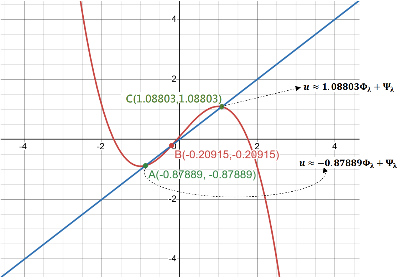
2.2 Multiplicity result based on a fixed point argument↩︎

For each \(r_i\in \boldsymbol{\mathrm{S}}_{\star}\), \(i=1,...,n\), where \(\mathcal{N}:\mathbb{R}\to\mathbb{R}\) satisfies (A3), we define a mapping \(\boldsymbol{\mathsf{T}}_{i,\lambda}:\mathcal{I}_{i,\lambda}\to\mathcal{I}_{i,\lambda}\) as follows:

\[\label{mapT} \boldsymbol{\mathsf{T}}_{i,\lambda}(\theta)= \boldsymbol{\mathsf{N}}[(r_i+\theta)\Phi_{\lambda}+\Psi_{\lambda}]-r_i,\quad\theta\in\mathcal{I}_{i,\lambda},\tag{12}\] where \(\mathcal{I}_{i,\lambda}\subset\mathbb{R}\) depending on \(\lambda\) is a closed set to be determined. The rationale behind this construction is that a fixed point of the mapping \(\boldsymbol{\mathsf{T}}_{i,\lambda}:\mathcal{I}_{i,\lambda}\to\mathcal{I}_{i,\lambda}\) (if it exists) corresponds to a solution of equation 5 with the boundary condition 2 . Specifically, if 12 admits a fixed point \(\theta_{i,\lambda}\), i.e., \[\boldsymbol{\mathsf{N}}[(r_i+\theta_{i,\lambda})\Phi_{\lambda}+\Psi_{\lambda}]=r_i+\theta_{i,\lambda}\] with \(\theta_{i,\lambda}\in\mathcal{I}_{i,\lambda}\), then from 9 we can see that each \(u_{i,\lambda}:=(r_i+\theta_{i,\lambda})\Phi_{\lambda}+\Psi_{\lambda}\) is a solution of equation 5 with the boundary condition 2 .

The main difficulty, therefore, lies in constructing appropriate closed sets \(\mathcal{I}_{i,\lambda}\subset\mathbb{R}\) for each \(i=1,...,n\). These sets must be chosen such that the mapping 12 admits a fixed point \(\theta_{i,\lambda}\in\mathcal{I}_{i,\lambda}\), and all \(r_i+\theta_{i,\lambda}\) remain distinct. Based on the asymptotic estimates of \(\Phi_{\lambda}\) and \(\Psi_{\lambda}\) as \(\lambda\to\infty\) (established in Section 4.1), we shall set \(\mathcal{I}_{i,\lambda}=:[-\lambda^{\frac{1-p}{4p}}, \lambda^{\frac{1-p}{4p}}]\) for each \(i=1,...,n\). We will then show that, under assumptions (A1)–(A3), the mapping \(\boldsymbol{\mathsf{T}}_{i,\lambda}\) defined by 12 is a well-defined contraction from \([-\lambda^{\frac{1-p}{4p}}, \lambda^{\frac{1-p}{4p}}]\) into itself for all sufficiently large \(\lambda>0\).

The proof of Proposition 2 is given in Section 4.2.

Proposition 2 guarantees the existence of a unique fixed point \(\theta_{i,\lambda}\in[-\lambda^{\frac{1-p}{4p}}, \lambda^{\frac{1-p}{4p}}]\). This, in turn, demonstrate that for sufficiently large \(\lambda>0\), equation 5 with the boundary condition 2 has multiple solutions. Our first main result on the multiplicity and qualitative properties of solutions is stated as follows.

Theorem 3(ii) states that equation 5 with the boundary condition 2 can admit an arbitrary finite number of distinct solutions. In this context, both the function \(\mathcal{N}\) and the parameter \(\lambda\) play a crucial role in determining the number of solutions. This result represents a distinctive characteristic of this class of linear equations with nonlocal nonlinearity. The proof of Theorem 3 is given in Section 4.3.

2.3 On the general case of multiple nonlocal nonlinearities↩︎

Based on the approach established in Sections 2.1–2.2, the main purpose of this study is to generalize 1 to a linear elliptic equation with multiple nonlocal terms, which is given by \[\label{eq-u2} -\nabla\cdot(\mathsf{D}(x)\nabla u) +\lambda f(x)u= \eta \sum_{j=1}^kh_j(x)\boldsymbol{\mathsf{N}}_j[u]+h_0(x) \quad\text{in}\,\,\Omega,\tag{15}\] where \(k\geq1\) and we make the following assumptions:

• For \(j=0,1,...,k\), the functions \(h_j\in\text{C}^{0}(\overline{\Omega};\mathbb{R})\) and \(\frac{h_j}{f}\in\text{C}^{2}(\overline{\Omega};\mathbb{R})\). In addition, there exists an interior point \(\boldsymbol{\mathrm{x}}_0\in\Omega\) where the set \(\{h_1(\boldsymbol{\mathrm{x}}_0),...,h_k(\boldsymbol{\mathrm{x}}_0)\}\) is linearly independent.

• Let \(w_j\in\mathrm{L}^p(\Omega)\) for some \(p>1\) be such that \(\int_\Omega w_j(y)\,\mathrm{d}y=1\). Let \(\mathcal{N}_j:\mathbb{R}\to\mathbb{R}\) be locally Lipschitz continuous. We define the nonlocal term \(\boldsymbol{\mathsf{N}}_j[u]\) analogously to 4 as follows: \[\label{N-2j} \boldsymbol{\mathsf{N}}_j[u]= \begin{cases} \displaystyle\int_\Omega w_j(y)\mathcal{N}_j(u(y))\,\mathrm{d}y& (\text{type~I}); \\ \displaystyle\mathcal{N}_j(\int_\Omega w_j(y)u(y)\,\mathrm{d}y) & (\text{type~II}). \end{cases}\tag{16}\] Furthermore, we assume that the set of functions \(\{w_1,...,w_k\}\) is linearly independent on \(\overline{\Omega}\). Similarly, the set of functions \(\{\mathcal{N}_1,...,\mathcal{N}_k\}\) is also linearly independent on \(\mathbb{R}\). These assumptions guarantee that the nonlocal terms \(\boldsymbol{\mathsf{N}}_j[u]\) cannot be combined or simplified.

To investigate the multiplicity of solutions to equation 15 with the boundary condition 2 , we will extend the methodology and argument established in Sections 2.1–2.2. Consider the following auxiliary equations: \[\label{eq-Phj} \begin{cases} -\nabla\cdot(\mathsf{D}(x)\nabla \Phi_{j,\lambda,\eta}) + \lambda f(x)\Phi_{j,\lambda,\eta}=\eta h_j(x) \quad&\text{in}\,\,\Omega,\\ \displaystyle\Phi_{j,\lambda,\eta}+b(x) \frac{\partial\Phi_{j,\lambda,\eta}}{\partial{\vec{\nu}}} = 0\quad&\text{on}\,\,\partial\Omega, \end{cases}\tag{17}\] for \(j=1,...,k\), and \[\label{eq-Ps0} \begin{cases} -\nabla\cdot(\mathsf{D}(x)\nabla \Psi_{0,\lambda}) + \lambda f(x)\Psi_{0,\lambda}=h_0(x) \quad&\text{in}\,\,\Omega,\\ \displaystyle\Psi_{0,\lambda}+b(x) \frac{\partial\Psi_{0,\lambda}}{\partial{\vec{\nu}}} = g(x)\quad&\text{on}\,\,\partial\Omega. \end{cases}\tag{18}\] Since \(f>0\), based on (A4) and 17 , we can easily deduce that the unique solutions \(\Phi_{1,\lambda,\eta}\),...,\(\Phi_{k,\lambda,\eta}\) are linearly independent. This, along with 18 , allows us to conclude that the representation \[\label{rp-u} u_{\lambda,\eta}(x)=\sum\limits_{j=1}^k\boldsymbol{\mathsf{N}}_j[u_{\lambda,\eta}]\Phi_{j,\lambda,\eta}(x)+\Psi_{0,\lambda}(x)\tag{19}\] solves equation 15 with the boundary condition 2 . Hence, the original multiplicity problem reduces to finding multiple solutions \(u\) to the implicit integral equation 19 with multiple nonlocal terms \(\boldsymbol{\mathsf{N}}_j[u_{\lambda,\eta}]\) for \(j=1,...,k\).

In what follows, we shall investigate the existence of multiple solutions to 19 . We define the vector-valued function \[\label{HN} \overrightarrow{\boldsymbol{\mathrm{H}}}(x):=\big\langle \frac{h_1(x)}{f(x)},...,\frac{h_k(x)}{f(x)} \big\rangle,\quad~x\in\overline{\Omega},\tag{20}\] and denote the inner product of vectors \(\vec{\boldsymbol{a}},\,\vec{\boldsymbol{b}}\in\mathbb{R}^k\) as \(\vec{\boldsymbol{a}}\boldsymbol{\cdot}\vec{\boldsymbol{b}}\), with the associated norm given by \(|\vec{\boldsymbol{a}}|=\sqrt{\vec{\boldsymbol{a}}\boldsymbol{\cdot}\vec{\boldsymbol{a}}}\). Under an asymptotic viewpoint and using fixed point arguments, we will show that the original multiplicity problem is now linked to the number of distinct solutions  \(\vec{\boldsymbol{\mathrm{r}}}\in\mathbb{R}^k\) of the following equation: \[\label{rNH} \vec{\boldsymbol{\mathrm{r}}}=\big\langle\boldsymbol{\mathsf{N}}_1\big[\vec{\boldsymbol{\mathrm{r}}}\boldsymbol{\cdot}\overrightarrow{\boldsymbol{\mathrm{H}}}\big],...,\boldsymbol{\mathsf{N}}_k\big[\vec{\boldsymbol{\mathrm{r}}}\boldsymbol{\cdot}\overrightarrow{\boldsymbol{\mathrm{H}}}\big] \big\rangle.\tag{21}\] By 16 , each \(\boldsymbol{\mathsf{N}}_j\big[\vec{\boldsymbol{\mathrm{r}}}\boldsymbol{\cdot}\overrightarrow{\boldsymbol{\mathrm{H}}}\big]\) is a real number independent of \(x\). As a result, 21 constitutes a system of algebraic equations for the unknown vector \(\vec{\boldsymbol{\mathrm{r}}}\).

Firstly, we consider the set \(\boldsymbol{\mathrm{S}}_k\) consisting of solutions \(\vec{\boldsymbol{\mathrm{r}}}\) to 21 with the following properties:

\[\label{sk} \boldsymbol{\mathrm{S}}_k= \left\{\vec{\boldsymbol{\mathrm{r}}}\in\mathbb{R}^k\left|\, \begin{align} &\vec{\boldsymbol{\mathrm{r}}}\,\,\text{satisfies}~(\ref{rNH}),\,\,\text{and~there~exists}~\delta_{\vec{\boldsymbol{\mathrm{r}}}}>0\,\,\text{such~that}\\ &|\mathcal{N}_j({s}_1)-\mathcal{N}_j({s}_2)|\leq\mathcal{L}_{\vec{\boldsymbol{\mathrm{r}}}}|{s}_1-{s}_2|,\,\,\text{for\,all}\, j=1,...,k,\\ &\text{whenever}\,\,||{s}_i-\vec{\boldsymbol{\mathrm{r}}}\boldsymbol{\cdot}\overrightarrow{\boldsymbol{\mathrm{H}}}||_{\mathrm{L}^{\infty}(\Omega)}<\delta_{\vec{\boldsymbol{\mathrm{r}}}},\text{ for }i=1,2. \end{align}\right.\right\},\tag{22}\] where \(\delta_{\vec{\boldsymbol{\mathrm{r}}}}\) depends on \(\vec{\boldsymbol{\mathrm{r}}}\), and each \(\mathcal{L}_{\vec{\boldsymbol{\mathrm{r}}}}\) satisfies \[\label{Lr} 0<\mathcal{L}_{\vec{\boldsymbol{\mathrm{r}}}}|\Omega|^{1-\frac{1}{p}}\max_{1\leq j\leq red}{k}||w_j||_{\mathrm{L}^{p}(\Omega)} <\frac{1}{k||\overrightarrow{\boldsymbol{\mathrm{H}}}||_{\mathrm{L}^{\infty}(\Omega)}}.\tag{23}\] Here, the \(\text{L}^\infty\)-norm of a \(k\)-dimensional vector-valued function is defined as the maximum of the \(\text{L}^\infty\)-norms of its \(k\) components.

In our subsequent analysis of the existence of multiple solutions to 19 , we assume the following regarding 22 :

• The set \(\boldsymbol{\mathrm{S}}_k\) has \(n\) distinct elements, where \(n\geq2\) and \(n\) can be infinite.

In Appendix (Section 7), we provide two examples to verify the validity of 23 and assumption (A6).

In Section 2.2, we have established the existence of multiple solutions for equation 5 with boundary condition 2 for sufficiently large \(\lambda\). This was achieved by combining fixed-point arguments and asymptotic analysis under assumption (A3) for the set \(\boldsymbol{\mathrm{S}}_{\star}\) defined in 10 . Based on these findings, we now proceed directly to define the following mapping on a suitable complete metric space (to be specified in the proof of Theorem 4): \[\label{nT} \boldsymbol{\Gamma}_{\vec{\boldsymbol{\mathrm{r}}},\lambda,\eta}(\vec{\boldsymbol{\vartheta}}) =\big\langle\boldsymbol{\mathsf{N}}_1\big[(\vec{\boldsymbol{\mathrm{r}}}+\vec{\boldsymbol{\vartheta}})\boldsymbol{\cdot}\overrightarrow{\boldsymbol{\Phi}}_{\lambda,\eta}+\Psi_{0,\lambda}\big],...,\boldsymbol{\mathsf{N}}_k\big[(\vec{\boldsymbol{\mathrm{r}}}+\vec{\boldsymbol{\vartheta}})\boldsymbol{\cdot}\overrightarrow{\boldsymbol{\Phi}}_{\lambda,\eta}+\Psi_{0,\lambda}\big] \big\rangle-\vec{\boldsymbol{\mathrm{r}}}\tag{24}\] where \[\label{vP} \overrightarrow{\boldsymbol{\Phi}}_{\lambda,\eta}:=\big\langle\Phi_{1,\lambda,\eta},...,\Phi_{k,\lambda,\eta}\big\rangle.\tag{25}\] We will prove that the mapping \(\boldsymbol{\Gamma}_{\vec{\boldsymbol{\mathrm{r}}},\lambda,\eta}\) is a contraction in a suitable complete metric space for sufficiently large \(\lambda\) and \(\eta\), thus admitting a fixed point \(\vec{\boldsymbol{\vartheta}}_{\vec{\boldsymbol{\mathrm{r}}},\lambda,\eta}\) (cf. Proposition 5 in Section 5). It follows from 24 that \[\label{nPh} \vec{\boldsymbol{\mathrm{r}}}+\vec{\boldsymbol{\vartheta}}_{\vec{\boldsymbol{\mathrm{r}}},\lambda,\eta}=\big\langle\boldsymbol{\mathsf{N}}_1\big[(\vec{\boldsymbol{\mathrm{r}}}+\vec{\boldsymbol{\vartheta}}_{\vec{\boldsymbol{\mathrm{r}}},\lambda,\eta})\boldsymbol{\cdot}\overrightarrow{\boldsymbol{\Phi}}_{\lambda,\eta}+\Psi_{0,\lambda}\big],...,\boldsymbol{\mathsf{N}}_k\big[(\vec{\boldsymbol{\mathrm{r}}}+\vec{\boldsymbol{\vartheta}}_{\vec{\boldsymbol{\mathrm{r}}},\lambda,\eta})\boldsymbol{\cdot}\overrightarrow{\boldsymbol{\Phi}}_{\lambda,\eta}+\Psi_{0,\lambda}\big] \big\rangle.\tag{26}\] Now we define \[\label{rtu} u_{\vec{\boldsymbol{\mathrm{r}}},\lambda,\eta}=(\vec{\boldsymbol{\mathrm{r}}}+\vec{\boldsymbol{\vartheta}}_{\vec{\boldsymbol{\mathrm{r}}},\lambda,\eta})\boldsymbol{\cdot}\overrightarrow{\boldsymbol{\Phi}}_{\lambda,\eta}+\Psi_{0,\lambda}.\tag{27}\] Combining 25 –26 with 27 yields \[u_{\vec{\boldsymbol{\mathrm{r}}},\lambda,\eta}=\sum\limits_{j=1}^k\boldsymbol{\mathsf{N}}_j\big[(\vec{\boldsymbol{\mathrm{r}}}+\vec{\boldsymbol{\vartheta}}_{\vec{\boldsymbol{\mathrm{r}}},\lambda,\eta})\boldsymbol{\cdot}\overrightarrow{\boldsymbol{\Phi}}_{\lambda,\eta}+\Psi_{0,\lambda}\big]\Phi_{j,\lambda,\eta}+\Psi_{0,\lambda}=\sum\limits_{j=1}^k\boldsymbol{\mathsf{N}}_j[u_{\vec{\boldsymbol{\mathrm{r}}},\lambda,\eta}]\Phi_{j,\lambda,\eta}+\Psi_{0,\lambda},\] which is precisely the form of 19 . As a consequence, \(u_{\vec{\boldsymbol{\mathrm{r}}},\lambda,\eta}\) defined in 27 forms a solution to equation 15 with the boundary condition 2 .

We will show that if \(\vec{\boldsymbol{\mathrm{r}}}\in\boldsymbol{\mathrm{S}}_k\), then for sufficiently large \(\lambda>0\), the mapping \(\vec{\boldsymbol{\mathrm{r}}}\mapsto u_{\vec{\boldsymbol{\mathrm{r}}},\lambda,\eta}\) is injective. This injectivity, along with assumption (A6), implies that the equation has at least \(n\) distinct solutions. The corresponding result is stated as follows.

The proof of Theorem 4 is given in Section 5.

3 Proof of Proposition 1↩︎

In this section, we state the proof of Proposition 1. For \(\Theta\in\mathbb{R}\), we consider the equation \[\label{veq} -\nabla\cdot(\mathsf{D}(x)\nabla v) +\lambda f(x)v=\eta \Theta h(x) \quad\text{in}\,\,\Omega,\tag{30}\] with the boundary condition \[\label{vbd} v+b(x) \frac{\partial v}{\partial{\vec{\nu}}} = g(x)\quad\text{on}\,\,\partial\Omega.\tag{31}\] Note that \(\Theta\) corresponds to the nonlocal term in 1 . For each \(\lambda,\eta>0\), by 3 and the standard elliptic regularity theorem [22], equation 30 –31 admits a unique solution \(v=v_{\lambda,\eta,\Theta}\in\text{C}^1(\overline{\Omega})\cap\text{C}^2(\Omega)\). This allows us to define a mapping \(T_{\lambda,\eta}:\mathbb{R}\to\mathbb{R}\) as \[\label{mto-v} T_{\lambda,\eta}(\Theta)=\boldsymbol{\mathsf{N}}[v_{\lambda,\eta,\Theta}].\tag{32}\] For \(\Theta_1,\,\Theta_2\in\mathbb{R}\), we shall claim:

• if \(b(x)\geq0\) on \(\partial\Omega\), then \[\label{app-t1} |T_{\lambda,\eta}(\Theta_1)-T_{\lambda,\eta}(\Theta_2)|\leq\frac{\eta\mathcal{L}\Omega|^{1-\frac{1}{p}}||w||_{\text{L}^{p}(\Omega)}}{\lambda}\max_{\overline{\Omega}}\frac{|h|}{f}|\Theta_1-\Theta_2|.\tag{33}\]

• if \(b(x)\equiv0\) on \(\partial\Omega\), then \[\label{app-t3} \begin{align} & |T_{\lambda,\eta}(\Theta_1)-T_{\lambda,\eta}(\Theta_2)|\\ \leq&\,\frac{\eta\mathcal{L}|\Omega|^{1-\frac{1}{p}}||w||_{\text{L}^{p}(\Omega)}\max_{\overline{\Omega}}|h|}{\left(\lambda\min_{\overline{\Omega}}f\right)^{\max\{\frac{1}{2},\frac{1}{p}\}}\left(\mathfrak{D}\Lambda_{\Omega}+\lambda\min_{\overline{\Omega}}f\right)^{1-\max\{\frac{1}{2},\frac{1}{p}\}}}|\Theta_1-\Theta_2|. \end{align}\tag{34}\]

For the case \(b(x)\geq0\) on \(\partial\Omega\), we see from ?? and 33 that \(T_{\lambda,\eta}:\mathbb{R}\to\mathbb{R}\) is a contraction mapping, which ensures the existence of a unique fixed point. In the special case where \(b(x)\equiv0\) on \(\partial\Omega\), it follows from ?? and 34 that the map also admits a unique fixed point. We use the same symbol \(\Theta_{\lambda,\eta}\) for the fixed point in both cases for simplicity. This fixed point satisfies the relation \[\Theta_{\lambda,\eta}=T_{\lambda,\eta}(\Theta_{\lambda,\eta})=\boldsymbol{\mathsf{N}}[v_{\lambda,\eta,\Theta_{\lambda,\eta}}].\] Using this result in combination with 30 –31 , we show that \(u=v_{\lambda,\eta,\Theta_{\lambda,\eta}}\) is a solution of 1 –2 .

It remains to prove the uniqueness of the solution to 1 –2 under the conditions on \(\lambda\) and \(\eta\) given by ?? . Suppose, for the sake of contradiction, that 1 –2 has two distinct solutions \(u_1^*\) and \(u_2^*\). We define \[\Theta_i^*:=\boldsymbol{\mathsf{N}}[u_i^*]\quad\text{and}\quad\,v_i^*:=v_{\lambda,\eta,\Theta_i},\,\,i=1,2.\] Then, by the uniqueness of 30 –31 , the solution corresponding to \(\Theta=\Theta_i^*\) is unique, so \(v_i^*\) must be equal to \(u_i^*\). Along with 32 , we have \[u_i^*=v_i^*\quad\text{and}\quad\Theta_i^*=\boldsymbol{\mathsf{N}}[v_i^*]=T_{\lambda,\eta}(\Theta_i^*),\quad~i=1,2.\] This shows that both \(\Theta_1^*\) and \(\Theta_2^*\) are fixed points of \(T_{\lambda,\eta}\) defined in 32 . Since \(T_{\lambda,\eta}\) is a contraction mapping with a unique fixed point over \(\mathbb{R}\), we conclude that \(\Theta_1^*=\Theta_2^*\). This, in turn, implies \(v_1^*=v_{\lambda,\eta,\Theta_1}=v_{\lambda,\eta,\Theta_2}=v_2^*\). As a consequence, we have \(u_1^*=v_1^*=v_2^*=u_2^*\) which is a contradiction to our initial assumption that the solutions were distinct. Therefore, we prove the uniqueness of the solution to 1 –2 and complete the proof of Proposition 1.

4 Proof of Proposition 2 and Theorem 3↩︎

4.1 Asymptotic estimates of \(\Phi_{\lambda}\) and \(\Psi_{\lambda}\)↩︎

Multiplying the equation in 6 by \(\Phi_{\lambda}-1\) and using 3 , one may check that \[\label{ch-8} \begin{align} \lambda (\Phi_{\lambda}-1)^2=&\,\frac{1}{f(x)}(\Phi_{\lambda}-1)\nabla\cdot(\mathsf{D}(x)\nabla \Phi_{\lambda}) \\ \leq&\,\frac{1}{f(x)}\left(\frac{1}{2}\nabla\cdot\left(\mathsf{D}(x)\nabla(\Phi_{\lambda}-1)^2\right)-\mathfrak{D}|\nabla\Phi_{\lambda}|^2\right)\\ \leq&\,\left(2\min_{\overline{\Omega}}f\right)^{-1}\nabla\cdot\left(\mathsf{D}(x)\nabla(\Phi_{\lambda}-1)^2\right)\quad\text{in}\,\,\Omega. \end{align}\tag{41}\]

We further establish a refined upper bound depending on \(\lambda>0\) for \(\Phi_{\lambda}\). According to 8 and 41 , we consider an auxiliary function \[\label{w-V} V(x)=\exp\left({-\mathfrak{M}_0\sqrt{\lambda}\mathsf{d}(x)}\right),\quad\,x\in\overline{\Omega},\tag{42}\] which is chosen to satisfy \(V\geq(\Phi_{\lambda}-1)^2\) on \(\partial\Omega\), where \(\mathsf{d}(x):=\text{dist}(x,\partial\Omega)\) and \(\mathfrak{M}_0\) (independent of \(\lambda\)) is a positive constant to be determined later. We will derive a differential inequality for \(V\) that matches the form of 41 . To do this, we first introduce a key concept for a rigorous argument, noting that the boundary \(\partial\Omega\) is smooth. This smoothness ensures that for a sufficiently small \(\delta>0\) (independent of \(\lambda\)), the subdomain \(\Omega_{\delta}=\{x\in\Omega\,|\,\mathsf{d}(x)<\delta\}\) is free from any focal points, and the distance function \(\mathsf{d}\in\text{C}^2(\overline{\Omega_{\delta}})\) (cf. [23]). Using 42 , we can establish estimates for \(\nabla\cdot\left(\nabla(V-(\Phi_{\lambda}-1)^2)\right)\) within \(\Omega_{\delta}\) and then choose a constant \(\mathfrak{M}_0\) such that \((\Phi_{\lambda}-1)^2(x)\leq {V}(x)\) for all \(x\in\overline{\Omega_{\delta}}\), provided \(\lambda\) is sufficiently large. Subsequently, a standard application of the maximum principle (since \(\min_{\overline{\Omega}}f>0\)) extends this result to the entire domain, yielding \((\Phi_{\lambda}-1)^2(x)\leq{V}(x)\) for all \(x\in\overline{\Omega}\). For simplicity, we will present a simplified argument by considering the case where \(\overline{\Omega}\) has no focal points and \(\mathsf{d}\in\text{C}^2(\overline{\Omega})\). Then, we have \(|\nabla\mathsf{d}(x)|=1\) for \(x\in\Omega\), which streamlines our analysis.

We now use the preceding arguments to derive detailed estimates. A direct computation, based on the fact from 42 that \(\nabla{V}=-\sqrt{\lambda}\mathfrak{M}_0{V}\nabla\mathsf{d}\) and \(|\nabla\mathsf{d}|=1\), yields \[\label{mkv} \begin{align} &\nabla\cdot\left(\mathsf{D}(x)\nabla{V}(x)\right)\\ =&\,\left[\lambda{\mathfrak{M}_0^2\nabla\mathsf{d}(x)\cdot\mathsf{D}(x)\cdot(\nabla\mathsf{d}(x))^T}-\sqrt{\lambda}\mathfrak{M}_0\nabla\cdot(\mathsf{D}(x)\nabla\mathsf{d}(x))\right]{V}(x)\\ \leq&\,\mathfrak{M}_1\left(\lambda{\mathfrak{M}_0^2}+\sqrt{\lambda}\mathfrak{M}_0\right){V}(x)\quad\text{in}\,\,\Omega, \end{align}\tag{43}\] where \((\nabla\mathsf{d})^T\) denotes the transpose of \(\nabla\mathsf{d}\) and \[\label{m11} \mathfrak{M}_1=\max\left\{\max_{1\leq i,j\leq {\color{black}m}}\max\limits_{\overline{\Omega}}|D_{ij}|,\max\limits_{\overline{\Omega}}\left|\nabla\cdot(\mathsf{D}\nabla\mathsf{d})\right|\right\}.\tag{44}\] From 41 and 43 –44 , we need to ensure a positive constant \(\mathfrak{M}_0\) such that \(\mathfrak{M}_1\left(\lambda{\mathfrak{M}_0^2}+\sqrt{\lambda}\mathfrak{M}_0\right)\leq2\lambda\min_{\overline{\Omega}}f\) holds for sufficiently large \(\lambda\). To fulfill this requirement, we can choose \[\label{ml0} \mathfrak{M}_0=\sqrt{\frac{1}{\mathfrak{M}_1}\min_{\overline{\Omega}}f}\,\,\text{and}\,\, \lambda\geq\frac{1}{\mathfrak{M}_0^2}.\tag{45}\] Then, a simple calculation shows the required estimate \[2\lambda\min_{\overline{\Omega}}f-\mathfrak{M}_1\left(\lambda{\mathfrak{M}_0^2}+\sqrt{\lambda}\mathfrak{M}_0\right)=\sqrt{\lambda}\left(\sqrt{\lambda}\min_{\overline{\Omega}}f-\mathfrak{M}_0\mathfrak{M}_1\right) \geq0.\] Under 45 , we thus arrive at \[\begin{align} 0&\,\leq-\nabla\cdot\left(\mathsf{D}(x)\nabla\left({V}-(\Phi_{\lambda}-1)^2\right)\right)\\ &\qquad\quad+ \mathfrak{M}_1\left(\lambda{\mathfrak{M}_0^2}+\sqrt{\lambda}\mathfrak{M}_0\right)V-2\lambda\min_{\overline{\Omega}}f(\Phi_{\lambda}-1)^2\\ &\,\leq2\lambda\min_{\overline{\Omega}}f\left({V}-(\Phi_{\lambda}-1)^2\right)\quad\text{in}\,\,\Omega. \end{align}\] Along with \(V\geq(\Phi_{\lambda}-1)^2\) on \(\partial\Omega\), we conclude that for \(\lambda\geq\frac{1}{\mathfrak{M}_0^2}\), the following estimate holds: \[\label{ch-9} |\Phi_{\lambda}(x)-1|\leq\sqrt{V(x)}=\exp\left({-\frac{\mathsf{d}(x)}{2}\mathfrak{M}_0\sqrt{\lambda}}\right),\quad\forall\,x\in\overline{\Omega}.\tag{46}\] Using 8 , we can apply the same argument as for 41 –46 to the equation 7 to obtain the estimate \[\label{ch-10} |\Psi_{\lambda}(x)|\leq\max_{\partial\Omega}|g|\exp\left({-\frac{\mathsf{d}(x)}{2}\mathfrak{M}_0\sqrt{\lambda}}\right),\quad\forall\,x\in\overline{\Omega},\tag{47}\] as \(\lambda\geq\frac{1}{\mathfrak{M}_0^2}\).

4.2 Proof of Proposition 2↩︎

Let \(r_i\in\boldsymbol{\mathrm{S}}_{\star}\) be fixed. Firstly, we need a lemma:

We will now show that for all sufficiently large \(\lambda>0\) (possibly depending on \(i\)), the mapping \(\boldsymbol{\mathsf{T}}_{i,\lambda}\) defined by 12 is a contraction from \([-\lambda^{\frac{1-p}{4p}}, \lambda^{\frac{1-p}{4p}}]\) into itself. As the arguments are similar to those provided in Lemma 1, it is sufficient to present a detailed proof for the case of Type I of 49 for clarity and rigor, i.e., \[\label{mapTt} \boldsymbol{\mathsf{T}}_{i,\lambda}(\theta)= \int_\Omega w(y)\left(\mathcal{N}((r_i+\theta)\Phi_{\lambda}(y)+\Psi_{\lambda}(y))-\mathcal{N}(r_i)\right)\,\mathrm{d}y,\quad\theta\in[-\lambda^{\frac{1-p}{4p}}, \lambda^{\frac{1-p}{4p}}].\tag{61}\]

For a given \(\lambda\geq\widetilde{\lambda}_{i,*}\) let \(\theta_1,\theta_2\in[-\lambda^{\frac{1-p}{4p}}, \lambda^{\frac{1-p}{4p}}]\). By 52 , we have \[(r_i+\theta_1)\Phi_{\lambda}(y)+\Psi_{\lambda}(y),\,\,(r_i+\theta_2)\Phi_{\lambda}(y)+\Psi_{\lambda}(y)\in(r_i-\delta_{r_i},r_i+\delta_{r_i}),\,\,\forall y\in\Omega\setminus\Omega_{\lambda^{-\frac{1}{3}}}.\] Consequently, applying 8 , 10 , 46 and 50 , we obtain \[\label{ch-24} \begin{align} &\int_{\Omega\setminus\Omega_{\lambda^{-\frac{1}{3}}}} |w(y)|\left|\mathcal{N}((r_i+\theta_1)\Phi_{\lambda}(y)+\Psi_{\lambda}(y))-\mathcal{N}((r_i+\theta_2)\Phi_{\lambda}(y)+\Psi_{\lambda}(y))\right|\,\mathrm{d}y\\ &\qquad\quad\quad \leq\mathcal{L}_{r_i}|\theta_1-\theta_2|\int_{\Omega\setminus\Omega_{\lambda^{-\frac{1}{3}}}}|w(y)|\Phi_{\lambda}(y)\,\mathrm{d}y \leq\mathcal{L}_{r_i}|\Omega|^{1-\frac{1}{p}}|w||_{\text{L}^{p}(\Omega)}|\theta_1-\theta_2|. \end{align}\tag{62}\] Here, a direct application of \(0\leq\Phi_{\lambda}\leq1\) and Hölder’s inequality yields the last estimate of 62 . On the other hand, since \(|(r_i+\theta_j)\Phi_{\lambda}(y)+\Psi_{\lambda}(y)|\leq|r_i|+\lambda^{\frac{1-p}{4p}}+ \max\limits_{\partial\Omega}|g|\) is uniformly bounded for \(\lambda\geq\widetilde{\lambda}_{i,*}\), by (A1), there exist finite numbers \(\widetilde{L}_{r_i}>0\) and \(\lambda_{i,*}\geq\widetilde{\lambda}_{i,*}\) such that, as \(\lambda\geq\lambda_{i,*}\), we have \[\label{ch-25} \begin{align} &\int_{\Omega_{\lambda^{-\frac{1}{3}}}} |w(y)|\left|\mathcal{N}((r_i+\theta_1)\Phi_{\lambda}(y)+\Psi_{\lambda}(y))-\mathcal{N}((r_i+\theta_2)\Phi_{\lambda}(y)+\Psi_{\lambda}(y))\right|\,\mathrm{d}y\\ &\qquad\quad \leq\widetilde{L}_{r_i}|\theta_1-\theta_2|\int_{\Omega_{\lambda^{-\frac{1}{3}}}}|w(y)|\Phi_{\lambda}(y)\,\mathrm{d}y \leq\widetilde{L}_{r_i}|\Omega_{\lambda^{-\frac{1}{3}}}|^{1-\frac{1}{p}}|w||_{\text{L}^{p}(\Omega)}|\theta_1-\theta_2|\\ &\qquad\quad\leq\frac{1}{2}\left(1-\mathcal{L}_{r_i}|\Omega|^{1-\frac{1}{p}}|w||_{\text{L}^{p}(\Omega)}\right)|\theta_1-\theta_2|. \end{align}\tag{63}\] The last estimate of 63 is trivially valid due to \(|\Omega_{\lambda^{-\frac{1}{3}}}|\xrightarrow{\lambda\to\infty}0\). Combining 61 with 62 –63 yields \[\begin{align} &| \boldsymbol{\mathsf{T}}_{i,\lambda}(\theta_1)- \boldsymbol{\mathsf{T}}_{i,\lambda}(\theta_2)| \\ \leq&\, \int_\Omega |w(y)|\left|\left(\mathcal{N}((r_i+\theta_1)\Phi_{\lambda}(y)+\Psi_{\lambda}(y))-\mathcal{N}((r_i+\theta_2)\Phi_{\lambda}(y)+\Psi_{\lambda}(y))\right)\right|\,\mathrm{d}y\\ \leq&\,\frac{1}{2}\left(1+\mathcal{L}_{r_i}|\Omega|^{1-\frac{1}{p}}||w||_{\text{L}^{p}(\Omega)}\right)|\theta_1-\theta_2|, \end{align}\] which is a contraction because of \(\mathcal{L}_{r_i}|\Omega|^{1-\frac{1}{p}}|w||_{\text{L}^{p}(\Omega)}<1\). The contraction mapping theorem thus guarantees that for all \(\lambda\geq\lambda_{i,*}\), \(\boldsymbol{\mathsf{T}}_{i,\lambda}:[-\lambda^{\frac{1-p}{4p}},\lambda^{\frac{1-p}{4p}}]\to[-\lambda^{\frac{1-p}{4p}},\lambda^{\frac{1-p}{4p}}]\) admits a unique fixed point \(\theta_{i,\lambda}\). Therefore, the proof of Proposition 2 is complete.

4.3 Proof of Theorem 3↩︎

We first consider the case where \(\boldsymbol{\mathrm{S}}_{\star}=\{r_1,...,r_n\}\) is finite, consisting of exactly \(n\) distinct elements. By Proposition 2 we have \(\boldsymbol{\mathsf{T}}_{i,\lambda}(\theta_{i,\lambda})=\theta_{i,\lambda}\) for some \(|\theta_{i,\lambda}|\leq\lambda^{\frac{1-p}{4p}}\), as \(\lambda\geq\lambda_{i,*}\). Together with 12 , this yields a solution \(u_{i,\lambda}=(r_i+\theta_{i,\lambda})\Phi_{\lambda}+\Psi_{\lambda}\) to equation 5 with the boundary condition 2 , satisfying \(\boldsymbol{\mathsf{N}}[u_{i,\lambda}]=r_i+\theta_{i,\lambda}\), for each \(i=1,...,n\). As a consequence, by 8 we have \[\label{bNu} \left| \boldsymbol{\mathsf{N}}[u_{i,\lambda}]-r_i \right|+\max_{\overline{\Omega}} |u_{i,\lambda}-(r_i\Phi_{\lambda}+\Psi_{\lambda})|\leq2|\theta_{i,\lambda}|\leq2\lambda^{\frac{1-p}{4p}}\xrightarrow{\lambda\to\infty}0.\tag{64}\] From (A3), we see that all \(r_i\) are independent of \(\lambda\) and satisfy \(r_i<r_{i+1}\), for \(i\in\{1,...,n-1\}\). We can then find a sufficiently large \(\lambda_{*}\geq\max\{\lambda_{i,*}|\,i=1,...,n\}\) such that \[\lambda_{*}^{\frac{1-p}{4p}}<\min\limits_{1\leq i\leq n-1}\frac{r_{i+1}-r_i}{2}.\] This guarantees \(r_i+\theta_{i,\lambda}<r_{i+1}+\theta_{i+1,\lambda}\) for \(i=1,...,n-1\), as \(\lambda\geq\lambda_{*}\).

On the other hand, by 3 we see that the solution \(\Phi_{\lambda}\) of 6 is positive in \(\Omega\). As a direct result, we immediately obtain \[u_{i+1,\lambda}-u_{i,\lambda}=[(r_{i+1}+\theta_{i+1,\lambda})-(r_i+\theta_{i,\lambda})]\Phi_{\lambda}>0\quad\text{in}\,\, \Omega.\] This shows that all solutions \(u_{i,\lambda}\) satisfying 13 are distinct when \(\lambda\geq\lambda_{*}\). Furthermore, 14 follows directly from 64 .

We now turn to the case where \(b(x)>0\) on \(\partial\Omega\), and claim that \(\min_{\overline{\Omega}}\Phi_{\lambda}>0\) for all \(\lambda>0\). This consequence is a direct application of Hopf lemma (cf. [26]). To prove this, we set \({\phi}_{\lambda}=1-\Phi_{\lambda}\). Applying the maximum principle to the equation of \({\phi}_{\lambda}\) with the condition 3 , we find that \({\phi}_{\lambda}\) must attain its maximum value at a boundary point \(x_{\text{b}}\in\partial\Omega\). Since the smoothness of \(\partial\Omega\) ensures that \(\Omega\) has the interior sphere property, it follows from [26] that \(\frac{\partial{\phi}_{\lambda}}{\partial{\vec{\nu}}}(x_{\text{b}})>0\). This is equivalent to \[\label{maxP} \min_{\overline{\Omega}}\Phi_{\lambda}=\Phi_{\lambda}(x_{\text{b}})=-b(x_{\text{b}})\frac{\partial\Phi_{\lambda}}{\partial{\vec{\nu}}}(x_{\text{b}})=b(x_{\text{b}})\frac{\partial{\phi}_{\lambda}}{\partial{\vec{\nu}}}(x_{\text{b}})>0.\tag{65}\] Consequently, the combination of 13 and 65 implies \(u_{i+1,\lambda}-u_{i,\lambda}=[(r_{i+1}+\theta_{i+1,\lambda})-(r_i+\theta_{i,\lambda})]\Phi_{\lambda}>0\) on \(\overline{\Omega}\). This completes the proof of Theorem 3(i).

Theorem 3(ii) is a direct consequence of Theorem 3(i). By considering a subset \(\{r_1,...,r_{\widetilde{n}}\}\) of \(\boldsymbol{\mathrm{S}}_{\star}\) such that \(r_1<\cdots<r_{\widetilde{n}}\) and following the same argument as in Theorem 3(i), we obtain that for each \(\lambda_{\widetilde{n}}>0\) such that as \(\lambda\geq\lambda_{\widetilde{n}}\) (for some \(\lambda_{\widetilde{n}}>0\)), the equation possesses at least \(\widetilde{n}\) distinct solutions of the form \((r_i+\theta_{i,\lambda})\Phi_{\lambda}+\Psi_{\lambda}\), for \(i=1,...,\widetilde{n}\). Consequently, the proof of Theorem 3 is complete.

5 Proof of Theorem 4↩︎

5.1 Asymptotic estimates of \(\Phi_{j,\lambda,\eta}\) and \(\Psi_{0,\lambda}\)↩︎

We first establish the asymptotic estimate of \(\Phi_{j,\lambda,\eta}\) and \(\Psi_{0,\lambda}\) with respect to the parameters \(\lambda\) and \(\eta\). By 3 and 20 , we can apply the standard maximum principle to 17 and obtain an upper bound of \(|\Phi_{j,\lambda,\eta}|\): \[\label{mPj} \max_{\overline{\Omega}}|\Phi_{j,\lambda,\eta}|\leq\frac{\eta}{\lambda}\max_{\overline{\Omega}}\frac{|h_j|}{f}\leq\frac{\eta}{\lambda}||\overrightarrow{\boldsymbol{\mathrm{H}}}||_{\mathrm{L}^{\infty}(\Omega)}.\tag{66}\] Rearranging the expression in 17 , we define a new function \(\widetilde{\Phi}_j\) for simplicity by setting \[\label{ch-pj} \widetilde{\Phi}_j:=\Phi_{j,\lambda,\eta}-\frac{\eta h_j(x)}{\lambda f(x)}.\tag{67}\] Under 67 and assumption (A4), we obtain equation of \(\widetilde{\Phi}_j\): \[\label{wPj} \frac{1}{\lambda}\nabla\cdot(\mathsf{D}(x)\nabla \widetilde{\Phi}_j) =f(x) \widetilde{\Phi}_j-\frac{\eta}{\lambda^2}\nabla\cdot\left(\mathsf{D}(x)\nabla \frac{h_j(x)}{f(x)}\right).\tag{68}\] For convenience, we omit the subscripts \(\lambda\) and \(\eta\) on \(\widetilde{\Phi}_j\) as we will only perform estimates in the subsequent analysis. Multiplying 68 by \(\widetilde{\Phi}_j\) and using the uniform ellipticity condition (see 3 -(a)), one may check that \[\label{6-ch} \begin{align} &\frac{1}{\lambda}\nabla\cdot\left(\mathsf{D}(x)\nabla \left(\widetilde{\Phi}_j^2-\frac{\eta^2}{\lambda^4}\mathfrak{M}_3^2\right)\right)\\ \geq&\,2\mathfrak{D}|\nabla\widetilde{\Phi}_j|^2+2f(x) \widetilde{\Phi}_j^2-\frac{2\eta}{\lambda^2}\widetilde{\Phi}_j\nabla\cdot\left(\mathsf{D}(x)\nabla \frac{h_j(x)}{f(x)}\right)\\ \geq&\,f(x) \left(\widetilde{\Phi}_j^2-\frac{\eta^2}{\lambda^4}\mathfrak{M}_{3,j}^2\right)\quad\text{in}\,\,\Omega, \\ \end{align}\tag{69}\] where we define \[\mathfrak{M}_{3,j}=\max_{\overline{\Omega}}\frac{1}{f}\left|\nabla\cdot\left(\mathsf{D}\nabla \frac{h_j}{f}\right)\right|,\quad j=0,1,...,k,\] which is a positive constant independent of \(\lambda\). Then by 20 , 66 and 69 , we can employ the same argument as in 41 –47 to obtain \[\widetilde{\Phi}_j^2(x)-\frac{\eta^2}{\lambda^4}\mathfrak{M}_{3,j}^2\leq\frac{\eta^2}{\lambda^2}\left(4||\overrightarrow{\boldsymbol{\mathrm{H}}}||_{\mathrm{L}^{\infty}(\Omega)}^2+ \frac{\mathfrak{M}_{3,j}^2}{\lambda^2}\right)\exp\left({-\mathsf{d}(x)\mathfrak{M}_0\sqrt{\lambda}}\right)\quad\text{in}\,\,\overline{\Omega},\] as \(\lambda\geq\frac{1}{\mathfrak{M}_0^2}\), where \(\mathfrak{M}_0\) is defined in 45 . Here the right-hand side of the above estimate is simplified by once again using the estimate \(\max_{\overline{\Omega}}\frac{|h_j|}{f}\leq||\overrightarrow{\boldsymbol{\mathrm{H}}}||_{\mathrm{L}^{\infty}(\Omega)}\). As a consequence, for \(j=1,...,k\), we arrive at \[\label{8-ch} \begin{align} &\left|\Phi_{j,\lambda,\eta}(x)-\frac{h_j(x)}{ f(x)}\right|\\ \leq&\,\frac{|\eta-\lambda|}{\lambda}\max_{\overline{\Omega}}\frac{|h_j|}{f}+| \widetilde{\Phi}_j(x)|\\ \leq&\,\frac{|\eta-\lambda|}{\lambda}||\overrightarrow{\boldsymbol{\mathrm{H}}}||_{\mathrm{L}^{\infty}(\Omega)}+\frac{\eta}{\lambda^2}\mathfrak{M}_{3,j}\\ &\,+\frac{\eta}{\lambda}\left(2||\overrightarrow{\boldsymbol{\mathrm{H}}}||_{\mathrm{L}^{\infty}(\Omega)}+ \frac{\mathfrak{M}_{3,j}}{\lambda}\right)\exp\left({-\frac{\mathsf{d}(x)}{2}\mathfrak{M}_0\sqrt{\lambda}}\right)\quad\text{in}\,\,\overline{\Omega}, \end{align}\tag{70}\] as \(\lambda\geq\frac{1}{\mathfrak{M}_0^2}\).

The solution \(\Psi_{0,\lambda}\) to 18 satisfies the maximum bound: \[\label{p0bd} \max_{\overline{\Omega}}|\Psi_{0,\lambda}|\leq\max\left\{\max_{\partial\Omega}|g|,\frac{1}{\lambda}\max_{\overline{\Omega}}\frac{|h_0|}{f}\right\}.\tag{71}\] We then proceed by applying the same argument as in 69 to \(\widetilde{\Psi}_0(x)=\Psi_{0,\lambda}(x)-\frac{h_0(x)}{\lambda f(x)}\), which yields \[\label{9-ch} \begin{align} \frac{1}{\lambda}\nabla\cdot(\mathsf{D}(x)\nabla \widetilde{\Psi}_0^2) \geq&\, f(x) \left(\widetilde{\Psi}_0^2-\frac{1}{\lambda^4f^2}\left|\nabla\cdot\left(\mathsf{D}(x)\nabla \frac{h_0(x)}{f(x)}\right)\right|^2\right)\\ \geq&\, f(x) \left(\widetilde{\Psi}_0^2-\frac{\mathfrak{M}_{3,0}^2}{\lambda^4}\right) \quad\text{in}\,\,\Omega. \end{align}\tag{72}\] Let us consider the case where \(g\neq0\) on \(\partial\Omega\). Hence, by applying the same argument as in 69 –70 to 72 and utilizing 71 , we arrive at the following estimate for \(\lambda\geq\max\{\frac{1}{\mathfrak{M}_0^2},\frac{\max_{\overline{\Omega}}\frac{|h_0|}{f}}{\max_{\partial\Omega}|g|}\}\): \[\label{10-ch} |\Psi_{0,\lambda}(x)|\leq\frac{1}{\lambda}\max_{\overline{\Omega}}\frac{|h_0|}{f}+\max_{\partial\Omega}|g|\exp\left({-\frac{\mathsf{d}(x)}{2}\mathfrak{M}_0\sqrt{\lambda}}\right),\quad\forall\,x\in\overline{\Omega}.\tag{73}\] When \(g\equiv0\) on \(\partial\Omega\), 73 holds for \(\lambda>0\), trivially due to 71 .

5.2 Completion of the proof of Theorem 4↩︎

To prove Theorem 4, we first consider the mapping \(\boldsymbol{\Gamma}_{\vec{\boldsymbol{\mathrm{r}}},\lambda,\eta}:{\boldsymbol{\mathrm{Q}}_{\lambda}}\to{\boldsymbol{\mathrm{Q}}_{\lambda}}\) defined in 24 . Here, we define the closed and complete metric space \[{\boldsymbol{\mathrm{Q}}_{\lambda}}:=\{\vec{\boldsymbol{\vartheta}}\in\mathbb{R}^k|\,\|\vec{\boldsymbol{\vartheta}}\|_{\ell^\infty}\leq\frac{\lambda^{\frac{1-p}{4p}}}{k}\}\] equipped with the standard maximum norm \(\|\cdot\|_{\ell^\infty}\) on \(\mathbb{R}^k\). We then introduce the following property:

Having Proposition 5 at hand, we now present the proof of Theorem 4.

6 Concluding remarks and outlook↩︎

In this work, we study the qualitative properties of linear elliptic equations with multiple nonlocal nonlinearities. These equations present significant challenges, as they are typically not amenable to standard variational methods and often fall outside the scope of classical elliptic theory. To address the difficulty in analysis, we developed a novel theoretical framework that integrates fixed-point arguments with asymptotic techniques. This approach establishes a new connection between asymptotic analysis and the existence and multiplicity theory of non-variational elliptic equations. Our methodology not only circumvents the absence of a variational structure but also uncovers a deeper understanding of how the interplay between parameters and nonlocal effects dictates the number of solutions.

Beyond a purely mathematical study, our work provides a new perspective on the fundamental nature of these nonlocal equations. The diverse asymptotics of solutions we have uncovered suggests that the interplay between parameters and nonlocal effects dictates not just existence, but also the very structure of these solutions. This finding is significant as it provides a new paradigm for understanding how nonlocality fundamentally alters the behavior of nonlocal elliptic equations, with potential implications for modeling complex phenomena in physics and biology.

Our findings contribute to a broader effort to understand the intricate interplay between locality and nonlocality in mathematical models of the physical systems. Furthermore, our results motivate a deeper exploration into the specific physical interpretations of the multiple solutions we have found. For instance, in applications like population dynamics or neural networks, these distinct solutions could correspond to different stable states or equilibrium patterns. We believe this work provides a solid foundation for future research and underscores the importance of developing new analytical tools for nonlocal problems. In the coming years, we expect this framework to be extended to investigate equations with more complex nonlocal terms or different boundary conditions.

7 Appendix: Validity of assumptions (A3) and (A6)↩︎

We will provide examples on the validity of assumptions (A3) and (A6), which are constructed by means of periodically perturbed functions.

Validity of assumption (A3). To demonstrate the validity of assumption (A3), we can consider a simplified case where \(w(y)=\frac{1}{|\Omega|}\). This choice satisfies assumption (A2) and implies that the condition on the Lipschitz constant in 10 becomes \(\mathcal{L}_r<\frac{|\Omega|^{\frac{1}{p}-1}}{||w||_{\mathrm{L}^{p}(\Omega)}}=1\). We now provide an example for 10 satisfying (A3) as follows.

• Consider a cubic polynomial \[\mathcal{N}(r)=r-\frac{2}{(r_1-r_2)^2}(r-r_1)(r-r_2)\left(r-\frac{r_1+r_2}{2}\right),\] where \(r_1\neq r_2\) are reals. Then the equation \(r=\mathcal{N}(r)\) has three distinct real roots \(r_1\), \(r_2\) and \(\frac{r_1+r_2}{2}\) satisfying \(\mathcal{N}'(r_1)=0\), \(\mathcal{N}'(r_2)=0\) and \(\mathcal{N}'(\frac{r_1+r_2}{2})=\frac{3}{2}\). It immediately follows \(\boldsymbol{\mathrm{S}}_{\star}=\{r_1,r_2\}\) for this specific case.

In fact, high-degree polynomials \(\mathcal{N}(r)\) that satisfy condition (A3) are frequently encountered.

For the reader’s reference, we provide examples (B2)–(B4) constructed from periodically perturbed functions to illustrate a case where the set \(\boldsymbol{\mathrm{S}}_{\star}\) contains infinitely many elements.

• For \(\mathcal{N}(r)=r+\sin r\), the roots of the equation \(r=\mathcal{N}(r)\) are given by \(j\pi\) for \(j\in\mathbb{Z}\). Although this \(\mathcal{N}:\mathbb{R}\to\mathbb{R}\) is globally Lipschitz continuous with an optimal constant of \(2\), a much tighter local Lipschitz condition holds in certain neighborhoods of the roots \(r_j=(2j-1)\pi\):³ \[|\mathcal{N}(s_1)-\mathcal{N}(s_2)|\leq \frac{1}{2}|s_1-s_2|~\text{for}~s_1,s_2\in(r_j-\frac{\pi}{3},r_j+\frac{\pi}{3}),~\forall i\in\mathbb{Z},\] which implies \(\boldsymbol{\mathrm{S}}_{\star}=\{(2j-1)\pi|\,j\in\mathbb{Z}\}\). This is an important example showing that even if \(\mathcal{N}:\mathbb{R}\to\mathbb{R}\) is globally Lipschitz continuous with Lipschitz constant large than \(\frac{|\Omega|^{\frac{1}{p}-1}}{||w||_{\mathrm{L}^{p}(\Omega)}}\), its corresponding set \(\boldsymbol{\mathrm{S}}_{\star}\) can still have infinitely many elements.

• Consider \[\mathcal{N}(r)=r+\alpha\text{e}^{-r^2}\sin r\quad\text{with}\,\,\alpha\in(0,1],\] for which the corresponding \(\boldsymbol{\mathrm{S}}_{\star}=\{(2j-1)\pi|\,j\in\mathbb{Z}\}\).

• Consider \(\mathcal{N}(r)=r+\xi(r)\), where \[\xi(r)= \begin{cases} \frac{1}{2}r(1-r),\quad\,r\in [0,1),\\ \frac{1}{2}(r-1)(r-2),\quad\,r\in[1,2), \end{cases}\] and extended periodically with a period of \(2\). In this case, \(\boldsymbol{\mathrm{S}}_{\star}=\{2j-1|\,j\in\mathbb{Z}\}\).

(B3) and (B4) can be straightforward to verify.

Validity of assumption (A6). We provide examples to demonstrate the validity of assumption (A6). For simplicity, we set \(k=2\) and let the functions \(w_1\) and \(w_2\) be defined on two disjoint subsets \(\Omega_1,\Omega_2\subset\Omega\) with \(|\Omega_1|=|\Omega_2|=\frac{1}{2}|\Omega|\), respectively, as follows: \[\label{ww} w_1(y)=\frac{2}{|\Omega|}\chi_{\Omega_1},\quad\, w_2(y)=\frac{2}{|\Omega|}\chi_{\Omega_2},\tag{94}\] where \(\chi_{\Omega_j}\) denotes the characteristic function on the set \(\Omega_j\), \(j=1,2\). 94 immediately implies that \(w_1\) and \(w_2\) are linearly independent and satisfy \(\int_{\Omega}w_1(y)\,\mathrm{d}y=\int_{\Omega}w_2(y)\,\mathrm{d}y=1\) and \(||w_1||_{\mathrm{L}^{p}(\Omega)}=||w_2||_{\mathrm{L}^{p}(\Omega)}=(\frac{|\Omega|}{2})^{\frac{1}{p}-1}\).

Next, we define the functions \(h_j\)’s and \(f\) as \[\label{hjf} \begin{cases} h_1(x)=f(x)+\gamma_1,\quad~h_2(x)=2f(x)+\gamma_2,\\ \text{where}\,\,f\not\equiv\text{constant}\,\,\text{on}\,\,\overline{\Omega},\,\,\text{and}\,\,\gamma_j\text{'s~are~constants~satisfying}\,\,\gamma_2\neq2\gamma_1. \end{cases}\tag{95}\] This ensures that \(h_1\) and \(h_2\) are linearly independent on the domain \(\overline{\Omega}\). On the other hand, the condition on all Lipschitz constants \(\mathcal{L}_{\vec{\boldsymbol{\mathrm{r}}}}\) in 23 reduces to \[\label{LH} 0<\mathcal{L}_{\vec{\boldsymbol{\mathrm{r}}}}<\frac{2^{\frac{1}{p}-3}}{||\overrightarrow{\boldsymbol{\mathrm{H}}}||_{\mathrm{L}^{\infty}(\Omega)}}\,\,\text{for~all}\,\, \vec{\boldsymbol{\mathrm{r}}}\in\boldsymbol{\mathrm{S}}_2.\tag{96}\]

Since by 20 and 95 , we have \(\overrightarrow{\boldsymbol{\mathrm{H}}}(x)-\langle 1,2\rangle=\langle \frac{\gamma_1}{f(x)},\frac{\gamma_2}{f(x)}\rangle\) on \(\overline{\Omega}\), we will construct \(\mathcal{N}_1\) and \(\mathcal{N}_2\) and determine the values of \(\gamma_1\) and \(\gamma_2\) such that any solution \(\vec{\boldsymbol{\mathrm{r}}}\in\mathbb{R}^2\) to the system \(\vec{\boldsymbol{\mathrm{r}}}=\big\langle{\mathcal{N}}_1\big(\vec{\boldsymbol{\mathrm{r}}}\boldsymbol{\cdot}\langle1,2\rangle\big),{\mathcal{N}}_2\big(\vec{\boldsymbol{\mathrm{r}}}\boldsymbol{\cdot}\langle1,2\rangle\big) \big\rangle\) is also a solution to the system \(\vec{\boldsymbol{\mathrm{r}}}=\big\langle\boldsymbol{\mathsf{N}}_1\big[\vec{\boldsymbol{\mathrm{r}}}\boldsymbol{\cdot}\overrightarrow{\boldsymbol{\mathrm{H}}}\big],\boldsymbol{\mathsf{N}}_2\big[\vec{\boldsymbol{\mathrm{r}}}\boldsymbol{\cdot}\overrightarrow{\boldsymbol{\mathrm{H}}}\big] \big\rangle\), i.e., \[\label{n1sn2} \begin{align} \small{ \{\vec{\boldsymbol{\mathrm{r}}}\in\mathbb{R}^2|\,\vec{\boldsymbol{\mathrm{r}}}=\big\langle{\mathcal{N}}_1\big(\vec{\boldsymbol{\mathrm{r}}}\boldsymbol{\cdot}\langle1,2\rangle\big),{\mathcal{N}}_2\big(\vec{\boldsymbol{\mathrm{r}}}\boldsymbol{\cdot}\langle1,2\rangle\big) \big\rangle\}\subseteq\{\vec{\boldsymbol{\mathrm{r}}}\in\mathbb{R}^2|\,\vec{\boldsymbol{\mathrm{r}}}=\big\langle\boldsymbol{\mathsf{N}}_1\big[\vec{\boldsymbol{\mathrm{r}}}\boldsymbol{\cdot}\overrightarrow{\boldsymbol{\mathrm{H}}}\big],\boldsymbol{\mathsf{N}}_2\big[\vec{\boldsymbol{\mathrm{r}}}\boldsymbol{\cdot}\overrightarrow{\boldsymbol{\mathrm{H}}}\big] \big\rangle\}. } \end{align}\tag{97}\] This enables the construction of the following examples (B5)–(B6) satisfying assumption (A6), which are a bit nontrivial.

• We consider \[\label{12N} \mathcal{N}_1(s)=-\frac{s}{2^{\rho}},\,\,\quad \mathcal{N}_2(s)=\frac{1+2^{\rho}}{2^{\rho+1}}\left(s-\frac{1+2^{\rho-1}}{1+2^{\rho}}(s-1)(s-2)(s-3)\right).\tag{98}\] We will show that for \[\label{rho6} \rho \geq6-\frac{1}{p},\tag{99}\] the setting of functions in 98 satisfies assumption (A6).

  Solving the system \(\vec{\boldsymbol{\mathrm{r}}}=\big\langle{\mathcal{N}}_1\big(\vec{\boldsymbol{\mathrm{r}}}\boldsymbol{\cdot}\langle1,2\rangle\big),{\mathcal{N}}_2\big(\vec{\boldsymbol{\mathrm{r}}}\boldsymbol{\cdot}\langle1,2\rangle\big) \big\rangle\) directly yields the set of solutions \(\{\vec{\boldsymbol{\mathrm{r}}}_1=\langle-\frac{1}{2^{\rho}},\frac{1+2^{\rho}}{2^{\rho+1}}\rangle,\vec{\boldsymbol{\mathrm{r}}}_2=2\vec{\boldsymbol{\mathrm{r}}}_1,\vec{\boldsymbol{\mathrm{r}}}_3=3\vec{\boldsymbol{\mathrm{r}}}_1\}\). It is clear that when \[\label{rho-ga} \gamma_1=\frac{1+2^{\rho}}{2}\gamma_2,\tag{100}\] there holds \(\vec{\boldsymbol{\mathrm{r}}}_j\boldsymbol{\cdot}\overrightarrow{\boldsymbol{\mathrm{H}}}=\vec{\boldsymbol{\mathrm{r}}}_j\boldsymbol{\cdot}\langle1,2\rangle\), for \(j=1,2,3\). Then by 16 , this implies that \(\vec{\boldsymbol{\mathrm{r}}}_j\) satisfy the system \(\vec{\boldsymbol{\mathrm{r}}}_j=\big\langle\boldsymbol{\mathsf{N}}_1\big[\vec{\boldsymbol{\mathrm{r}}}_j\boldsymbol{\cdot}\overrightarrow{\boldsymbol{\mathrm{H}}}\big],\boldsymbol{\mathsf{N}}_2\big[\vec{\boldsymbol{\mathrm{r}}}_j\boldsymbol{\cdot}\overrightarrow{\boldsymbol{\mathrm{H}}}\big] \big\rangle\) for \(j=1,2,3\). Hence, we have checked that 97 holds. A simple calculation yields \[\begin{cases} \displaystyle |{\mathcal{N}}_1'|\equiv\frac{1}{2^{\rho}},\,\, |{\mathcal{N}}_2'\big(\vec{\boldsymbol{\mathrm{r}}}_1\boldsymbol{\cdot}\langle1,2\rangle\big)| =|{\mathcal{N}}_2'\big(\vec{\boldsymbol{\mathrm{r}}}_3\boldsymbol{\cdot}\langle1,2\rangle\big)|=\frac{1}{2^{\rho+1}},\\ \displaystyle{\mathcal{N}}_2'\big(\vec{\boldsymbol{\mathrm{r}}}_2\boldsymbol{\cdot}\langle1,2\rangle\big)=\frac{1+3\cdot2^{\rho-1}}{2^{\rho+1}}. \end{cases}\] By 96 and 100 , we set \(\gamma_1\) and \(\gamma_2\), and require the property of \(f\) as follows: \[\label{b-g} \begin{cases} \displaystyle \gamma_2=-1,~\gamma_1=-\frac{1+2^{\rho}}{2}~\text{and}~f~\text{satisfies}\\ \min\limits_{\overline{\Omega}}f=2^{\rho-3}~\&~\max\limits_{\overline{\Omega}}f=2^{\rho-3}+1. \end{cases}\tag{101}\] A direct calculation yields \(||\overrightarrow{\boldsymbol{\mathrm{H}}}||_{\mathrm{L}^{\infty}(\Omega)}=\frac{3\cdot2^{\rho}+12}{2^{\rho}-8}\).

  Under 99 , we claim that \(\boldsymbol{\mathrm{S}}_2\supseteq\{\vec{\boldsymbol{\mathrm{r}}}_1,\vec{\boldsymbol{\mathrm{r}}}_3\}\) and \(\mathcal{L}_{\vec{\boldsymbol{\mathrm{r}}}_j}=2^{-\rho}\) for \(j=1,3\) satisfy 96 . This can be rigorously demonstrated by noting that \(||\overrightarrow{\boldsymbol{\mathrm{H}}}||_{\mathrm{L}^{\infty}(\Omega)}<8\) for \(\rho\geq4\), which further implies \[{2^{\frac{1}{p}-3}}{||\overrightarrow{\boldsymbol{\mathrm{H}}}||_{\mathrm{L}^{\infty}(\Omega)}^{-1}}-2^{-\rho}>2^{\frac{1}{p}-6}-2^{-\rho}\geq0~\text{for}~\rho\geq6-\frac{1}{p}.\] Consequently, \(\boldsymbol{\mathrm{S}}_2\supseteq\{\vec{\boldsymbol{\mathrm{r}}}_1,\vec{\boldsymbol{\mathrm{r}}}_3\}\) has at least two distinct elements that satisfy assumption (A6).

• As another example, let \(\mathcal{N}_1\) be as defined in 98 . We replace \(\mathcal{N}_2\) from 98 with a periodically perturbed function \[\mathcal{N}_2(s)=\frac{1+2^{\rho}}{2^{\rho+1}}\left(s-\frac{1-2^{\rho}}{1+2^{\rho}}\mathsf{k}\sin\frac{s}{\mathsf{k}}\right),\] where \(\mathsf{k}\) is a nonzero constant. Moreover, under assumptions 99 –100 and 101 , it is straightforward to solve the system \(\vec{\boldsymbol{\mathrm{r}}}=\big\langle{\mathcal{N}}_1\big(\vec{\boldsymbol{\mathrm{r}}}\boldsymbol{\cdot}\langle1,2\rangle\big),{\mathcal{N}}_2\big(\vec{\boldsymbol{\mathrm{r}}}\boldsymbol{\cdot}\langle1,2\rangle\big) \big\rangle\) and show that the corresponding set \[\boldsymbol{\mathrm{S}}_2\supseteq\{\left\langle-\frac{2\mathsf{z}-1}{2^\rho}\mathsf{k}\pi,\frac{(1+2^\rho)(2\mathsf{z}-1)}{2^{\rho+1}}\mathsf{k}\pi\right\rangle|\,\mathsf{z}\in\mathbb{Z}\}\] contains infinitely many elements.

Acknowledgement↩︎

This work was supported by the National Science and Technology Council of Taiwan under Grant 114-2115-M-007-013-MY2. The author expresses sincere gratitude to the anonymous referees for the insightful comments that greatly improved the original manuscript.

References↩︎

---

1. (cf. [24]) The volume of the tubular neighborhood \(\Omega_{\mu}\) admits the following asymptotic expansion \[|\Omega_{\mu}| = \mu|\partial\Omega| - \frac{\mu^2}{2}\sum_{i=1}^{m-1}\int_{\partial\Omega} \kappa_i(x)\, \text{d}\mathcal{H}^{m-1} + O(\mu^3),\quad\text{as}\,\,\mu\to 0^+,\] where \(\kappa_i(x)\)’s, \(i=1,...,m-1\), are the principal curvatures at \(x\in\partial\Omega\).↩︎

2. We obtain 59 by a similar argument to that for [21], and therefore omit the detailed proof.↩︎

3. Note that \(\mathcal{N}'((2j-1)\pi)=0\). This estimate is only used to align with the definition of the set \(\boldsymbol{\mathrm{S}}_{\star}\) in 10 .↩︎