Compensated Splitting For Generalized Lyapunov Equations
June 20, 2026
Abstract
The generalized Lyapunov equation has a natural splitting that leads to the standard fixed-point iteration (sFPI) for its numerical solution. sFPI is convergent, for an arbitrarily given initial guess, if and only if the spectral radius of the associated linear operator is smaller than \(1\). This means that sFPI may diverge if the spectral radius is \(1\) or bigger. In this paper, we propose a compensated splitting scheme that aims to reduce the spectral radius so that the resulting compensated fixed-point iteration (cFPI) has a better convergence property, namely, cFPI may still converge even if sFPI does not or cFPI converges faster than sFPI does when the latter is also convergent. Numerical results are presented to demonstrate the superiority of cFPI to sFPI.
Keywords: generalized Lyapunov equation, compensated splitting, fixed-point iteration, spectral radius
Mathematics Subject Classification 65F45, 65F08, 15A06, 15A24
1 Introduction↩︎
Our focus in this paper is the numerical solution to the generalized Lyapunov equation \[\label{eq:genlyap} AX + XA^{\mathop{\mathrm{H}}} + \sum_{j=1}^{m}N_j X N_j^{\mathop{\mathrm{H}}} + BB^{\mathop{\mathrm{H}}} = 0,\tag{1}\] where the matrices \(A, N_j\in\mathbb{C}^{n\times n}\) and \(B\in\mathbb{C}^{n\times \ell}\) with usually \(\ell\ll n\). Such an equation often arises from the model order reduction of bilinear control systems and linear parameter-varying systems, the stability analysis of linear stochastic differential equations, as well as the linearization of stochastic continuous-time algebraic Riccati equations [1]–[5]. The constant term in 1 takes such a special form \(BB^{\mathop{\mathrm{H}}}\) because of the sources of the generalized Lyapunov equation in applications. As far as the development in this paper is concerned, the constant term can be replaced with any square matrix \(C\). Imposing that \(C\) is Hermitian will generally imply that the solution \(X\) is Hermitian, too. In most existing literature, all matrices in 1 are assumed to be real, but we let them be complex for generality and that all matrices are real is simply a special case.
Theoretically, 1 is an \(n^2\)-by-\(n^2\) linear system of equations and can be turn into the familiar standard form of a linear system of equations: \[\label{eq:GLyap2ST} \mathscr{A}\mathop{\mathrm{vec}}(X)\equiv\Big[I_n\otimes A+\bar{A}\otimes I_n+\sum_{j=1}^m\bar{N}_j\otimes N_j\Big]\mathop{\mathrm{vec}}(X)=-\mathop{\mathrm{vec}}(BB^{\mathop{\mathrm{H}}}),\tag{2}\] where \(\otimes\) is the matrix Kronecker product, \(\bar{A}\) and \(\bar{N}_j\) denote the entrywise complex conjugate of \(A\) and \(N_j\), and \(\mathop{\mathrm{vec}}(\cdot)\) vectorizes a matrix into a column vector by stacking up the columns of the matrix. It follows from this standard form that if \(\mathscr{A}\in\mathbb{C}^{n^2\times n^2}\) is nonsingular then 1 has a unique solution and the solution \(X\) is Hermitian, but it is not clear if \(X\) is definite or not. Another implication of 2 is the temptation to solve the original 1 via 2 . Unfortunately, any direct solver such as variants of Gaussian elimination and is not feasible unless \(n\) is very small (a few tens) because of its \(O(n^4)\) storage and \(O(n^6)\) computational complexity [6], [7]. Usual iterative methods for linear systems [6], [8], [9] are straightforwardly applicable without the need to form \(\mathscr{A}\) explicitly.
The generalized Lyapunov equation 1 has received increasing attention over the last decades. The simplest numerical method is through the fixed-point technique, and it is based on splitting the linear terms in \(X\) in 1 naturally into \(\mathscr{M}(X)=\mathscr{N}(X)-BB^{\mathop{\mathrm{H}}}\), where \[\label{eq:NatSplit} \mathscr{M}(X):=AX + XA^{\mathop{\mathrm{H}}}, \quad \mathscr{N}(X)=-\sum_{j=1}^{m}N_j X N_j^{\mathop{\mathrm{H}}}.\tag{3}\] Both \(\mathscr{M}(\cdot)\) and \(\mathscr{N}(\cdot)\) are linear operators from \(\mathbb{C}^{n\times n}\) to itself, and in particular, \(\mathscr{N}(X)\preceq 0\) (negative semidefinite) for any \(X\succeq 0\) (positive semidefinite). When \(\mathscr{M}\) is invertible, such a splitting yields the following standard fixed-point iteration (sFPI): given \(X_0\), for \(k=1,2,\ldots\) solve \[\label{eq:NatItn} \mathscr{M}(X_k)\equiv AX_k+X_kA^{\mathop{\mathrm{H}}}=\mathscr{N}(X_{k-1})-BB^{\mathop{\mathrm{H}}}\tag{4}\] for \(X_k\) until convergence. Suppose that \(\mathscr{M}\) is invertible. A sufficient condition for the convergence of sFPI 4 is \[\label{eq:nat-rho601} \rho(\mathscr{M}^{-1}\mathscr{N})<1,\tag{5}\] where \(\rho(\mathscr{M}^{-1}\mathscr{N})\) is the spectral radius of \(\mathscr{M}^{-1}\mathscr{N}\) as a linear operator in \(\mathbb{C}^{n\times n}\). The condition implies that necessarily \[\mathscr{M}-\mathscr{N}=\mathscr{M}\,(\mathop{\mathrm{Id}}-\mathscr{M}^{-1}\mathscr{N})\] is invertible, where \(\mathop{\mathrm{Id}}\) denotes the identity operator in \(\mathbb{C}^{n\times n}\). But, if \(\rho(\mathscr{M}^{-1}\mathscr{N})\ge 1\), then the scheme is in general divergent. Our goal in this paper is to rectify \(\rho(\mathscr{M}^{-1}\mathscr{N})\ge 1\) to yield a new iterative scheme that may still converge. Roughly speaking, \(\rho(\mathscr{M}^{-1}\mathscr{N})\ge 1\) is caused by the \(\mathscr{N}\)-part being relative too “heavy”. Hence in order to overcome the violation, we have to take out a portion of the \(\mathscr{N}\)-part to compensate the \(\mathscr{M}\)-part. For that purpose, we propose to somehow decompose the \(\mathscr{N}\)-part as \[\label{eq:scrN-split} -\mathscr{N}(X)=EX+XE^{\mathop{\mathrm{H}}}-\widetilde{\mathscr{N}}(X)\tag{6}\] in such a way that \(\widetilde{\mathscr{N}}(\cdot)\) is made relatively less “heavy” than before and then compensate \(\mathscr{M}(X)\) with \(EX+XE^{\mathop{\mathrm{H}}}\), leading to \[\label{eq:t-scrMscrN} \mathscr{M}(X)-\mathscr{N}(X)=\underbrace{[\mathscr{M}(X)+EX+XE^{\mathop{\mathrm{H}}}]}_{=:\widetilde{\mathscr{M}}(X)}-\widetilde{\mathscr{N}}(X),\tag{7}\] which we will call a compensated splitting. As a result, we can establish the following compensated fixed-point iteration (cFPI): given \(X_0\), for \(k=1,2,\ldots\) solve \[\label{eq:NatItn-pert} \widetilde{\mathscr{M}}(X_k)\equiv (A+E)X_k+X_k(A+E)^{\mathop{\mathrm{H}}}=\widetilde{\mathscr{N}}(X_{k-1})-BB^{\mathop{\mathrm{H}}}\tag{8}\] for \(X_k\) until convergence. An ideal compensated splitting 7 should minimize \(\rho(\widetilde{\mathscr{M}}^{-1}\widetilde{\mathscr{N}}\,)\) subject to \(\widetilde{\mathscr{M}}\) being invertible. Conceivably, seeking such an ideal compensated splitting is utterly impractical. Instead, we seek somehow to “minimize” \(\widetilde{\mathscr{N}}(\cdot)\) optimally in certain sense. In the end, we come up with an optimal \(E\) that takes a very elegant form \[\label{eq:optimal40E41:intro} E=\frac{1}{n(1+\mu)}\sum_{j=1}^m\mathop{\mathrm{tr}}(\bar{N}_{j})\left[N_j -\frac{1}{2n} \mathop{\mathrm{tr}}(N_{j})\cdot I_n\right],\tag{9}\] where \(\mathop{\mathrm{tr}}(\cdot)\) takes the trace of a matrix, and \(\mu\ge 0\) is a regularizing parameter to control the magnitude of \(E\). How it is derived will be detailed in 2.
FPI-type methods are simple to design and implement. Beyond such methods as we have discussed so far, not surprisingly, modern iterative techniques for linear systems (see, e.g., [6]–[9]) have seen their extensions to the generalized Lyapunov equation 1 , including, for example, the bilinear ADI method [1], the greedy low-rank methods [10], Krylov subspace-type methods [11], and exploitations of the fixed-point iteration [12], a residual-based generalized rational-Krylov-type subspace method [13], and a method based on the Sherman–Morrison–Woodbury formula [3]. However, in this paper we will be focusing solely on rescuing sFPI from its divergence or making it converge faster. Any potential combination of the key idea of this paper with the state-of-the-art subspace-based projection techniques will be investigated in forthcoming studies.
The rest of this paper is organized as follows. In 2, a compensated splitting is proposed and its main result is 9 . Numerical experiments are reported in 3, demonstrating the new method’s superiority to sFPI. Finally, we draw conclusion and make comments in 4.
Notation. \(\mathbb{R}^{m\times n}\) and \(\mathbb{C}^{m\times n}\) denote the sets of real and complex \(m\times n\) matrices, respectively; \(\mathbb{R}^n=\mathbb{R}^{n\times1}\) and \(\mathbb{C}^n=\mathbb{C}^{n\times1}\), and \(I_n\in\mathbb{R}^{n\times n}\) is the identity matrix. For a matrix \(X\), \(X^{\mathop{\mathrm{T}}}\) and \(X^{\mathop{\mathrm{H}}}\) denote its transpose and complex conjugate transpose, respectively, and \(\|X\|_2\) and \(\|X\|_{\mathop{\mathrm{F}}}\) are the spectral and Frobenius norms of \(X\). Other notation will be defined at its first appearance.
2 Compensated Splitting↩︎
As we discussed in section 1, an ideal compensated splitting 7 should make \(\rho(\widetilde{\mathscr{M}}^{-1}\widetilde{\mathscr{N}}\,)\) as small as possible. Unfortunately, that is not numerically feasible, and so we will have to be less ambitious. We start by making \(\widetilde{\mathscr{N}}(X)\) as insignificant as possible over all \(X\in\mathbb{C}^{n\times n}\) and seek \(E\in\mathbb{C}^{n\times n}\) by \[\label{eq:SARE-CS} \min_E\,\max_{\|\mathop{\mathrm{vec}}(X)\|_2\le 1}\Bigl\|\sum_{j=1}^m N_jXN_j^{\mathop{\mathrm{H}}}-(EX+XE^{\mathop{\mathrm{H}}})\Bigr\|_{\mathop{\mathrm{F}}}^2+\mu\|EX+XE^{\mathop{\mathrm{H}}}\|_{\mathop{\mathrm{F}}}^2,\tag{10}\] where \(\mu\|EX+XE^{\mathop{\mathrm{H}}}\|_{\mathop{\mathrm{F}}}^2\) can be regarded as a regularization term on \(E\) to keep it from being too “big”, and \(\mu\ge 0\) is the regularizing parameter that has to be chosen properly. Notice that \[\begin{gather} \label{eq:SARE-CS39} \max_{\|\mathop{\mathrm{vec}}(X)\|_2\le 1}\Bigl\|\Bigl(I_n\otimes E+\bar E\otimes I_n-\sum_{j=1}^{m}\bar N_j\otimes N_j\Bigr)\mathop{\mathrm{vec}}(X)\Bigr\|_2^2 +\mu\|(I_n\otimes E+\bar E\otimes I_n)\mathop{\mathrm{vec}}(X)\|_2^2 \\ \le\Bigl\|I_n\otimes E+\bar E\otimes I_n-\sum_{j=1}^{m}\bar N_j\otimes N_j\Bigr\|_2^2 +\mu\|I_n\otimes E+\bar E\otimes I_n\|_2^2, \end{gather}\tag{11}\] which involves the sum of two spectral norms of two \(n^2\times n^2\) matrices, and conceivably minimizing the expression in 11 over \(E\) is a difficult thing to do, if at all possible. Instead, we relax 11 to \[\label{eq:SARE-CS3939} \min_E\Bigl\{f(E):=\Bigl\|I_n\otimes E+\bar E\otimes I_n-\sum_{j=1}^{m}\bar N_j\otimes N_j\Bigr\|_{\mathop{\mathrm{F}}}^2 +\mu\|I_n\otimes E+\bar E\otimes I_n\|_{\mathop{\mathrm{F}}}^2\Bigr\}.\tag{12}\] It can be seen that the objective \(f(E)\) in 15 is a non-negative quadratic function in the entries of \(E\) and it is convex. Hence any stationary point of 12 is a global minimum point. Our main result in this section is stated in the following theorem, where \(\mathop{\mathrm{tr}}(\cdot)\) takes the trace of a square matrix.
Theorem 1. An optimal \(E\) to 12 is given by \[\label{eq:optimal40E41:cpx} E=\frac{1}{n(1+\mu)}\sum_{j=1}^m\mathop{\mathrm{tr}}(\bar{N}_{j})\left[N_j -\frac{1}{2n} \mathop{\mathrm{tr}}(N_{j})\cdot I_n\right].\qquad{(1)}\] Moreover, the minimizer is unique for the real case, and for the complex case this optimal \(E\) is the one with the smallest Frobenius norm.
We will defer the proof of this theorem to subsections 2.1 and 2.2 below. A couple of immediately questions are: 1) what is the invertibility of the operator \(\widetilde{\mathscr{M}}\)? 2) does \(E\) in ?? always decrease the spectral radius in question? The answers to both questions are negative, as our later numerical experiments in 3 suggest. The following identity may provide some understanding as to when \(E\) in ?? will work better. \[\label{eq:trE} \mathop{\mathrm{tr}}(E)=\frac{1}{2n(1+\mu)}\sum_{j=1}^m|\mathop{\mathrm{tr}}(N_j)|^2\ge 0.\tag{13}\] Suppose that the magnitudes of all \(N_j\) are small and then so is that of \(E\) in ?? , and thus \(E\) can be considered a perturbation. Since \(\mathop{\mathrm{tr}}(A+E)=\mathop{\mathrm{tr}}(A)+\mathop{\mathrm{tr}}(E)\ge\mathop{\mathrm{tr}}(A)\), \(E\) will move some of the eigenvalues rightward. Now if the eigenvalues of \(A\) lie in the left-half plane, then collectively these eigenvalues will be moved rightward towards \(0\), making \(\widetilde{\mathscr{M}}\) “less invertible” than \(\mathscr{M}\). In such a case there is a possibility that any gain in “minimizing” \(\widetilde{\mathscr{N}}\) may get offset by worsening in \(\widetilde{\mathscr{M}}\) along the way. On the other hand, if the eigenvalues of \(A\) lie in the right-half plane, then collectively the eigenvalues of \(A\) will also be moved rightward but further away from \(0\), making \(\widetilde{\mathscr{M}}\) even “more invertible”. In such a situation, determining \(E\) by 12 has an implicit effect of serving the purpose of what an ideal compensated splitting 7 should achieve. This quantitative explanation is actually reflected in our numerical experiments in 3.
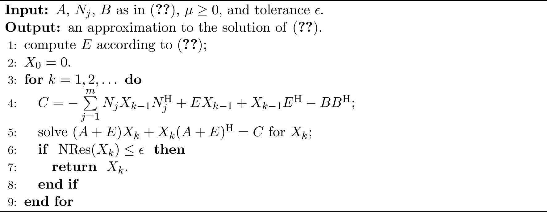
Now with the optimal \(E\) in 1, we create a compensated splitting in 7 and numerically the fixed-point iterative scheme 8 which we will call the compensated fixed-point iteration (cFPI), as outlined in 1, where all inner Lyapunov equations have the same coefficient matrix \(A+E\) and, hence, if solved by the Bartels-Stewart algorithm [14], the Schur decomposition of \(A+E\) can be computed outside the for-loop. In the algorithm, the normalized residual \(\mathop{\mathrm{NRes}}(\cdot)\) is defined as \[\label{eq:residual} \mathop{\mathrm{NRes}}(X) :=\frac{\Big\|A X+ X A^{\mathop{\mathrm{H}}} + \sum_{j=1}^{m}N_j X N_j^{\mathop{\mathrm{H}}} + BB^{\mathop{\mathrm{H}}}\Big\|_{\mathop{\mathrm{F}}}}{\|X\|_{\mathop{\mathrm{F}}}(2\|A\|_2+\sum_{j=1}^m\|N_j\|_2^2)+\|BB^{\mathop{\mathrm{H}}}\|_{\mathop{\mathrm{F}}}}.\tag{14}\] Since the spectral norm \(\|\cdot\|_2\) is computationally nontrivial, we will replace \(\|A\|_2\) with \(\sqrt{\|A\|_1\|A\|_{\infty}}\), and similarly for \(\|N_j\|_2\). These replacements should work equally well numerically because what is important is the correct magnitude of \(\mathop{\mathrm{NRes}}(\cdot)\).
In the next two subsections, we will establish ?? . In theory, the real case is a special one of the complex case when all involved matrices are real matrices. Hence there is no need to consider the real case separately if we can handle the complex case. It turns out that the real case is so much simpler and often the generalized Lyapunov equations 1 in applications are real ones, so we will single out the real case first and dive into the complex case separately. Notation \(E_{(s,t)}\) stands for the \((s,t)\)th entry of \(E\) and similarly for \((N_j)_{(s,t)}\).
2.1 Optimal \(E\) for the Real Case↩︎
Consider \(E\in\mathbb{R}^{n\times n}\) and so are all \(N_j\). We have \[\begin{align} \label{eq:obj:real} f(E)&=\sum_{s=1}^n\Bigl\|E+E_{(s,s)} I_n-\sum_{j=1}^m(N_j)_{(s,s)}N_j\Bigr\|_{\mathop{\mathrm{F}}}^2 +\mu\sum_{s=1}^n\Bigl\|E+E_{(s,s)} I_n\Bigr\|_{\mathop{\mathrm{F}}}^2 \nonumber \\ &\quad +\sum_{\begin{subarray}{c} s,t=1\\ s\ne t \end{subarray}}^n\Bigl\|E_{(s,t)} I_n-\sum_{j=1}^m(N_j)_{(s,t)} N_j\Bigr\|_{\mathop{\mathrm{F}}}^2 +\mu\sum_{\begin{subarray}{c} s,t=1\\ s\ne t \end{subarray}}^n\Bigl\|E_{(s,t)} I_n\Bigr\|_{\mathop{\mathrm{F}}}^2. \end{align}\tag{15}\] We start by finding the stationary points of 12 . To that end, it suffices to set the partial derivatives of \(f\) with respect to each entry of \(E\) to \(0\). We have, for \(s,t=1,2,\ldots, n\) and \(s\ne t\), \[\tag{16} \begin{align} 0&=\frac{1}{4}\frac{\partial f(E)}{\partial E_{(s,s)}}\nonumber\\ &=\frac{1}{4}\frac{\partial }{\partial E_{(s,s)}}\Bigl\|E+E_{(s,s)} I_n-\sum_{j=1}^m(N_j)_{(s,s)}N_j\Bigr\|_{\mathop{\mathrm{F}}}^2 +\mu\frac{1}{4}\frac{\partial }{\partial E_{(s,s)}}\Bigl\|E+E_{(s,s)} I_n\Bigr\|_{\mathop{\mathrm{F}}}^2\nonumber\\ &\quad +\frac{1}{4}\frac{\partial }{\partial E_{(s,s)}} \sum_{i=1,\, i\ne s}^n\Bigl\|E+E_{(i,i)} I_n-\sum_{j=1}^m(N_j)_{(i,i)}N_j\Bigr\|_{\mathop{\mathrm{F}}}^2 +\mu\frac{1}{4}\frac{\partial }{\partial E_{(s,s)}} \sum_{i=1,\, i\ne s}^n\Bigl\|E+E_{(i,i)} I_n\Bigr\|_{\mathop{\mathrm{F}}}^2\nonumber\\ &=\frac{1}{2}\Bigl[2E_{(s,s)}-\sum_{j=1}^m\big[(N_j)_{(s,s)}\big]^2\Bigr]2 +\frac{1}{2} \sum_{i=1,\, i\ne s}^n\Bigl[E_{(i,i)}+E_{(s,s)}-\sum_{j=1}^m(N_j)_{(s,s)}(N_j)_{(i,i)}\Bigr] \nonumber\\ &\quad+\mu\frac{1}{2}\Bigl[2E_{(s,s)}\Bigr]2 +\mu\frac{1}{2}\sum_{i=1,\, i\ne s}^n\Bigl[E_{(i,i)}+E_{(s,s)}\Bigr] \nonumber\\ &\quad+\frac{1}{2} \sum_{i=1,\, i\ne s}^n \Bigl[E_{(s,s)}+E_{(i,i)}-\sum_{j=1}^m(N_j)_{(i,i)}(N_j)_{(s,s)}\Bigr] +\mu\frac{1}{2} \sum_{i=1,\, i\ne s}^n \Bigl[E_{(s,s)}+E_{(i,i)}\Bigr] \nonumber\\ &=(n+1)(1+\mu)E_{(s,s)}+(1+\mu)\sum_{i=1,\, i\ne s}^n E_{(i,i)}-\sum_{j=1}^m(N_j)_{(s,s)}\sum_{i=1}^n(N_j)_{(i,i)} \nonumber\\ &=n(1+\mu) E_{(s,s)}+(1+\mu)\sum_{i=1}^n E_{(i,i)}-\sum_{j=1}^m(N_j)_{(s,s)}\mathop{\mathrm{tr}}(N_j), \tag{17} \\ 0&=\frac{1}{2}\frac{\partial f(E)}{\partial E_{(s,t)}}\nonumber\\ &=\frac{1}{2}\frac{\partial }{\partial E_{(s,t)}} \sum_{i=1}^n\Bigl\|E+E_{(i,i)} I_n-\sum_{j=1}^m(N_j)_{(i,i)}N_j\Bigr\|_{\mathop{\mathrm{F}}}^2 +\mu\frac{1}{2}\frac{\partial }{\partial E_{(s,t)}} \sum_{i=1}^n\Bigl\|E+E_{(i,i)} I_n\Bigr\|_{\mathop{\mathrm{F}}}^2\nonumber\\ &\quad + \frac{1}{2}\frac{\partial }{\partial E_{(s,t)}}\Bigl\|E_{(s,t)} I_n-\sum_{j=1}^m(N_j)_{(s,t)} N_j\Bigr\|_{\mathop{\mathrm{F}}}^2 +\mu\frac{1}{2}\frac{\partial }{\partial E_{(s,t)}}\Bigl\|E_{(s,t)} I_n\Bigr\|_{\mathop{\mathrm{F}}}^2\nonumber\\ &=\sum_{i=1}^n\Bigl[(1+\mu)E_{(s,t)}-\sum_{j=1}^m(N_j)_{(i,i)}(N_j)_{(s,t)}\Bigr]+ \sum_{i=1}^n \Bigl[(1+\mu)E_{(s,t)}-\sum_{j=1}^m(N_j)_{(s,t)}(N_j)_{(i,i)}\Bigr] \nonumber\\ &=2n(1+\mu)E_{(s,t)}-2\sum_{j=1}^m(N_j)_{(s,t)}\mathop{\mathrm{tr}}(N_j). \tag{18} \end{align}\] First we solve the system of \(n\) equations in 17 for \(1\le s\le n\) for the diagonal entries of \(E\). Sum up the \(n\) equations over \(s=1,2,\ldots, n\) to get \[\label{eq:partialf40E41:diag39} 2n(1+\mu)\sum_{s=1}^n E_{(s,s)}-\sum_{j=1}^m[\mathop{\mathrm{tr}}(N_j)]^2=0 \quad\Rightarrow\quad \sum_{s=1}^n E_{(s,s)}=\frac{1}{2n(1+\mu)}\sum_{j=1}^m[\mathop{\mathrm{tr}}(N_j)]^2.\tag{19}\] Plugging 19 into 17 , we find \[\label{eq:optimal40E41:diag:real} E_{(s,s)}=\frac{1}{n(1+\mu)} \left[\sum_{j=1}^m(N_j)_{(s,s)}\mathop{\mathrm{tr}}(N_j) -\frac{1}{2n}\sum_{j=1}^m[\mathop{\mathrm{tr}}(N_j)]^2\right]\quad for s=1,2,\ldots, n.\tag{20}\] Consider now the off-diagonal entries of \(E\). By 18 , we have for \(s,\,t=1,2,\ldots, n\) and \(s\ne t\), yielding \[\label{eq:optimal40E41:offdiag:real} E_{(s,t)}=\frac{1}{n(1+\mu)}\sum_{j=1}^m(N_j)_{(s,t)}\mathop{\mathrm{tr}}(N_j)\quad for s,\,t=1,2,\ldots, n and s\ne t.\tag{21}\] Putting 20 and 21 together, compactly, we have ?? for the real case. Since there is one and only one stationary point given by 20 and 21 together, and the optimizer must be the global minimizer.
2.2 Optimal \(E\) for the Complex Case↩︎
Consider the case when \(E\) and all \(N_j\) are complex. We have \[\begin{align} f(E) &=\sum_{s=1}^n\Bigl\|E+\bar{E}_{(s,s)} I_n-\sum_{j=1}^m(\bar{N}_j)_{(s,s)}N_j\Bigr\|_{\mathop{\mathrm{F}}}^2 +\mu\sum_{s=1}^n\Bigl\|E+\bar{E}_{(s,s)} I_n\Bigr\|_{\mathop{\mathrm{F}}}^2 \\ &\quad +\sum_{\begin{subarray}{c} s,t=1\\ s\ne t \end{subarray}}^n\Bigl\|\bar{E}_{(s,t)} I_n-\sum_{j=1}^m(\bar{N}_j)_{(s,t)} N_j\Bigr\|_{\mathop{\mathrm{F}}}^2 +\mu\sum_{\begin{subarray}{c} s,t=1\\ s\ne t \end{subarray}}^n\Bigl\|\bar{E}_{(s,t)} I_n\Bigr\|_{\mathop{\mathrm{F}}}^2. \end{align}\] To find the optimal \(E\) to 12 , we will find its stationary points determined by setting the partial derivatives of \(f\) with respect to the real and imaginary parts of each entry of \(E\) to \(0\). Write \[E_{(s,t)} = E_{(s,t)}^{{\rm re}} + \iota E_{(s,t)}^{{\rm im}}, \quad \bar{E}_{(s,t)} = E_{(s,t)}^{{\rm re}} - \iota E_{(s,t)}^{{\rm im}},\] where \(\iota\) is the imaginary unit, and \(E_{(s,t)}^{{\rm re}},\,E_{(s,t)}^{{\rm im}}\in\mathbb{R}\). It is known that \[\label{eq:diff-realE-imagE} \frac{\partial f(E)}{\partial E_{(s,t)}^{{\rm re}}} = \frac{\partial f(E)}{\partial E_{(s,t)}} + \frac{\partial f(E)}{\partial \bar{E}_{(s,t)}}, \quad \frac{1}{\iota}\cdot\frac{\partial f(E)}{\partial E_{(s,t)}^{{\rm im}}} = \frac{\partial f(E)}{\partial E_{(s,t)}} - \frac{\partial f(E)}{\partial \bar{E}_{(s,t)}},\tag{22}\] in which \(E\) and \(\bar{E}\) are treated as independent matrix variables. For the diagonal entries, we have \[\tag{23} \begin{align} \frac{\partial f(E)}{\partial E_{(s,s)}} &=\frac{\partial }{\partial E_{(s,s)}} \Bigl\|E+\bar{E}_{(s,s)} I_n-\sum_{j=1}^m(\bar{N}_j)_{(s,s)}N_j\Bigr\|_{\mathop{\mathrm{F}}}^2 +\mu\frac{\partial }{\partial E_{(s,s)}} \Bigl\|E+\bar{E}_{(s,s)} I_n\Bigr\|_{\mathop{\mathrm{F}}}^2 \nonumber \\ &\quad + \frac{\partial }{\partial E_{(s,s)}} \sum_{i=1,\,i\ne s}^n \Bigl\|E+\bar{E}_{(i,i)} I_n-\sum_{j=1}^m(\bar{N}_j)_{(i,i)}N_j\Bigr\|_{\mathop{\mathrm{F}}}^2 +\mu \frac{\partial }{\partial E_{(s,s)}} \sum_{i=1,\,i\ne s}^n \Bigl\|E+\bar{E}_{(i,i)} I_n\Bigr\|_{\mathop{\mathrm{F}}}^2 \nonumber\\ &= \frac{\partial }{\partial E_{(s,s)}} \Bigl| E_{(s,s)} + \bar{E}_{(s,s)} - \sum_{j=1}^m (\bar{N}_j)_{(s, s)}(N_j)_{(s, s)}\Bigr|^2\nonumber \\ & + \frac{\partial }{\partial E_{(s,s)}} \sum_{i=1,\,i\ne s}^n \Bigl|E_{(i, i)} + \bar{E}_{(s,s)} - \sum_{j=1}^m (\bar{N}_j)_{(s, s)}(N_j)_{(i,i)} \Bigr|^2 \nonumber \\ &\quad+\mu\frac{\partial }{\partial E_{(s,s)}} \Bigl| E_{(s,s)} + \bar{E}_{(s,s)}\Bigr|^2 + \mu\frac{\partial }{\partial E_{(s,s)}} \sum_{i=1,\,i\ne s}^n \Bigl|E_{(i, i)} + \bar{E}_{(s,s)} \Bigr|^2 \nonumber \\ &\quad + \frac{\partial }{\partial E_{(s,s)}} \sum_{i=1,\,i\ne s}^n \Bigl|E_{(s, s)} + \bar{E}_{(i, i)} - \sum_{j=1}^m (\bar{N}_j)_{(i, i)}(N_j)_{(s, s)} \Bigr|^2\nonumber \\ &\quad+\mu \frac{\partial }{\partial E_{(s,s)}} \sum_{i=1,\,i\ne s}^n \Bigl|E_{(s, s)} + \bar{E}_{(i, i)} \Bigr|^2 \nonumber \\ & = 2\Bigl[E_{(s,s)} + \bar{E}_{(s,s)} - \sum_{j=1}^m (\bar{N}_j)_{(s, s)}(N_j)_{(s, s)}\Bigr] \nonumber \\ & +\sum_{i=1,\,i\ne s}^n \Bigl[ E_{(i, i)} + \bar{E}_{(s,s)} - \sum_{j=1}^m (\bar{N}_j)_{(s, s)}(N_j)_{(i,i)} \Bigr] \nonumber \\ &\quad+\mu 2\Bigl[E_{(s,s)} + \bar{E}_{(s,s)} \Bigr] +\mu\sum_{i=1,\,i\ne s}^n \Bigl[ E_{(i, i)} + \bar{E}_{(s,s)} \Bigr] \nonumber \\ &\quad +\sum_{i=1,\,i\ne s}^n \Bigl[ \bar{E}_{(s, s)} + E_{(i, i)} - \sum_{j=1}^m (N_j)_{(i, i)}(\bar{N}_j)_{(s, s)} \Bigr] +\mu\sum_{i=1,\,i\ne s}^n \Bigl[ \bar{E}_{(s, s)} + E_{(i, i)} \Bigr] \nonumber \\ & = 2\sum_{i=1}^n \Bigl[ (1+\mu)\bigl(\bar{E}_{(s, s)} + E_{(i, i)}\bigr) - \sum_{j=1}^m (N_j)_{(i, i)}(\bar{N}_j)_{(s, s)} \Bigr] \nonumber \\ &=2n(1+\mu)\bar{E}_{(s,s)}+2(1+\mu)\sum_{i=1}^nE_{(i, i)} -2\sum_{j=1}^m \mathop{\mathrm{tr}}(N_j)\,(\bar{N}_j)_{(s, s)} , \tag{24} \\ \frac{\partial f(E)}{\partial \bar{E}_{(s,s)}} & =\frac{\partial }{\partial \bar{E}_{(s,s)}} \Bigl\|E+\bar{E}_{(s,s)} I_n-\sum_{j=1}^m(\bar{N}_j)_{(s,s)}N_j\Bigr\|_{\mathop{\mathrm{F}}}^2 +\mu\frac{\partial }{\partial \bar{E}_{(s,s)}} \Bigl\|E+\bar{E}_{(s,s)} I_n\Bigr\|_{\mathop{\mathrm{F}}}^2 \nonumber \\ &\quad+ \frac{\partial }{\partial E_{(s,s)}} \sum_{i=1,\,i\ne s}^n \Bigl\|E+\bar{E}_{(i,i)} I_n-\sum_{j=1}^m(\bar{N}_j)_{(i,i)}N_j\Bigr\|_{\mathop{\mathrm{F}}}^2 + \mu\frac{\partial }{\partial E_{(s,s)}} \sum_{i=1,\,i\ne s}^n \Bigl\|E+\bar{E}_{(i,i)} I_n\Bigr\|_{\mathop{\mathrm{F}}}^2 \nonumber\\ & =\frac{\partial }{\partial \bar{E}_{(s,s)}} \Bigl|E_{(s, s)} + \bar{E}_{(s, s)} - \sum_{j=1}^m (\bar{N}_j)_{(s, s)}(N_j)_{(s, s)}\Bigr|^2 \nonumber \\ & + \frac{\partial }{\partial \bar{E}_{(s,s)}} \sum_{i=1,\,i\ne s}^n \Bigl|E_{(i, i)} + \bar{E}_{(s,s)} - \sum_{j=1}^m (\bar{N}_j)_{(s,s)}(N_j)_{(i,i)} \Bigr|^2\nonumber \\ &\quad+\mu\frac{\partial }{\partial \bar{E}_{(s,s)}}\Bigl|E_{(s, s)} + \bar{E}_{(s, s)}\Bigr|^2 +\mu \frac{\partial }{\partial \bar{E}_{(s,s)}} \sum_{i=1,\,i\ne s}^n\Bigl|E_{(i, i)} + \bar{E}_{(s,s)} \Bigr|^2\nonumber \\ &\quad + \frac{\partial }{\partial \bar{E}_{(s,s)}} \sum_{i=1,\,i\ne s}^n \Bigl|\bar{E}_{(s, s)} + E_{(i, i)} - \sum_{j=1}^m (N_j)_{(i, i)}(\bar{N}_j)_{(s, s)} \Bigr|^2\nonumber \\ &\quad +\mu \frac{\partial }{\partial \bar{E}_{(s,s)}} \sum_{i=1,\,i\ne s}^n \Bigl|\bar{E}_{(s, s)} + E_{(i, i)} \Bigr|^2\nonumber \\ &=2\Bigl[ E_{(s, s)} + \bar{E}_{(s, s)} - \sum_{j=1}^m (\bar{N}_j)_{(s, s)}(N_j)_{(s, s)}\Bigr] \nonumber \\ & + \sum_{i=1,\,i\ne s}^n \Bigl[ \bar{E}_{(i, i)} + E_{(s, s)} - \sum_{j=1}^m (N_j)_{(s,s)}(\bar{N}_j)_{(i,i)} \Bigr] \nonumber \\ &\quad +\mu 2\Bigl[ E_{(s, s)} + \bar{E}_{(s, s)}\Bigr] + \mu\sum_{i=1,\,i\ne s}^n \Bigl[ \bar{E}_{(i, i)} + E_{(s, s)} \Bigr] \nonumber \\ &\quad + \sum_{i=1,\,i\ne s}^n \Bigl[ E_{(s, s)} + \bar{E}_{(i, i)} - \sum_{j=1}^m (\bar{N}_j)_{(i, i)}(N_j)_{(s, s)} \Bigr] +\mu \sum_{i=1,\,i\ne s}^n \Bigl[ E_{(s, s)} + \bar{E}_{(i, i)} \Bigr] \nonumber \\ &=2\sum_{i=1}^n \Bigl[ (1+\mu)\bigl(E_{(s, s)} + \bar{E}_{(i, i)}\bigr) - \sum_{j=1}^m (\bar{N}_j)_{(i, i)}(N_j)_{(s, s)} \Bigr] \nonumber \\ &= 2n(1+\mu) E_{(s, s)}+2(1+\mu)\sum_{i=1}^n\bar{E}_{(i, i)} -2\sum_{j=1}^m \mathop{\mathrm{tr}}(\bar{N}_j)\,(N_j)_{(s, s)}. \tag{25} \end{align}\] According to 22 and upon using 23 , the first order optimality condition on the diagonal entries of \(E\) is given by, for \(1\le s\le n\), \[\tag{26} \begin{align} 0&=\frac{\partial f(E)}{\partial E_{(s,s)}^{{\rm re}}} = \frac{\partial f(E)}{\partial E_{(s,s)}}+\frac{\partial f(E)}{\partial \bar{E}_{(s,s)}} \nonumber \\ &= 2n(1+\mu)\big[E_{(s, s)}+\bar{E}_{(s, s)}\big] +2(1+\mu)\sum_{i=1}^n\big[E_{(i, i)}+\bar{E}_{(i, i)}\big] -4\sum_{j=1}^m\Re\big( \mathop{\mathrm{tr}}(\bar{N}_j)\,(N_j)_{(s, s)}\big) \nonumber \\ &=4n(1+\mu) E_{(s, s)}^{{\rm re}}+4(1+\mu)\sum_{i=1}^nE_{(i, i)}^{{\rm re}} -4\sum_{j=1}^m\Re\big( \mathop{\mathrm{tr}}(\bar{N}_j)\,(N_j)_{(s, s)}\big), \tag{27} \\ 0&=\frac{1}{\iota}\cdot\frac{\partial f(E)}{\partial E_{(s,s)}^{{\rm im}}} = \frac{\partial f(E)}{\partial E_{(s,s)}} - \frac{\partial f(E)}{\partial \bar{E}_{(s,s)}} \nonumber \\ &=-2n(1+\mu)\big[E_{(s,s)}-\bar{E}_{(s,s)}\big] +2(1+\mu)\sum_{i=1}^n\big[E_{(i, i)}-\bar{E}_{(i, i)}\big] +2\iota\sum_{j=1}^m\Im\big(\mathop{\mathrm{tr}}(\bar{N}_j)\,(N_j)_{(s, s)}\big) \nonumber \\ &=-2n(1+\mu)\iota E_{(s,s)}^{{\rm im}}+2(1+\mu)\iota \sum_{i=1}^nE_{(i, i)}^{{\rm im}} +2\iota\sum_{j=1}^m\Im\big(\mathop{\mathrm{tr}}(\bar{N}_j)\,(N_j)_{(s, s)}\big), \tag{28} \end{align}\] where \(\Re(\cdot)\) and \(\Im(\cdot)\) take the real and imaginary parts of a complex number, respectively.
First we solve 27 for \(1\le s\le n\). Summing up 27 over \(1\le s\le n\), we get, after simplifications, \[\begin{align} &8n(1+\mu)\sum_{i=1}^n E_{(i,i)}^{{\rm re}} = 4\sum_{j=1}^m\mathop{\mathrm{tr}}(\bar{N}_j) \mathop{\mathrm{tr}}(N_{j}) \nonumber \\ \Rightarrow\quad& \sum_{i=1}^n E_{(i,i)}^{{\rm re}} = \frac{1}{2n(1+\mu)}\sum_{j=1}^m \mathop{\mathrm{tr}}(\bar{N}_j) \mathop{\mathrm{tr}}(N_{j}). \label{eq:KKT-diag-Re:sum} \end{align}\tag{29}\] Plug 29 into 27 to get, for \(s=1,2,\ldots,n\), \[\label{eq:optimal40E41:diag-Re} E_{(s,s)}^{{\rm re}} =\frac{1}{n(1+\mu)}\left[\sum_{j=1}^m\Re\big( (N_j)_{(s,s)} \mathop{\mathrm{tr}}(\bar{N}_{j})\big) -\frac{1}{2n}\sum_{j=1}^m \mathop{\mathrm{tr}}(\bar{N}_j) \mathop{\mathrm{tr}}(N_{j})\right].\tag{30}\] Next, we solve 28 for \(1\le s\le n\), which can be simplified to \[\label{eq:KKT-diag-Im39} -n E_{(s,s)}^{{\rm im}}+ \sum_{i=1}^nE_{(i, i)}^{{\rm im}} =-\sum_{j=1}^m\Im\big(\mathop{\mathrm{tr}}(\bar{N}_j)\,(N_j)_{(s, s)}\big) \quadfor 1\le s\le n,\tag{31}\] or, compactly, \[\label{eq:KKT-diag-Im3939} \begin{bmatrix} n-1 & -1 & \cdots & -1\\ -1 & n-1 & \cdots & -1\\ \vdots & \vdots & \ddots & \vdots \\ -1 & -1& \cdots & n-1 \end{bmatrix} \begin{bmatrix} E_{(1,1)}^{{\rm im}} \\ E_{(2,2)}^{{\rm im}} \\ \vdots \\ E_{(n,n)}^{{\rm im}} \end{bmatrix} =\frac{1}{1+\mu}\sum_{j=1}^m \begin{bmatrix} \Im\big( (N_j)_{(1,1)} \mathop{\mathrm{tr}}(\bar{N}_{j}) \big) \\ \Im\big( (N_j)_{(2,2)} \mathop{\mathrm{tr}}(\bar{N}_{j}) \big) \\ \vdots \\ \Im\big( (N_j)_{(n,n)} \mathop{\mathrm{tr}}(\bar{N}_{j}) \big) \end{bmatrix}:=\pmb{b},\tag{32}\] whose coefficient matrix has rank \(n-1\) and can be compactly expressed as \[C=n \Big(I_n-\frac{1}{n}\pmb{e}\pmb{e}^{\mathop{\mathrm{T}}}\Big),\] where \(\pmb{e}\in\mathbb{R}^n\) is the vector of all ones. We make a couple of observations:
1) the linear system 32 is consistent because the range of \(C\) is the orthogonal complement of \({\rm span}\{\pmb{e}\}\) and \(\pmb{b}\) is in the orthogonal complement: \[(1+\mu)\pmb{e}^{\mathop{\mathrm{T}}}\pmb{b}=\sum_{j=1}^m\sum_{i=1}^n\Im\big((N_j)_{(i,i)} \mathop{\mathrm{tr}}(\bar{N}_{j})\big) = \sum_{j=1}^m\Im\big(\mathop{\mathrm{tr}}(N_{j})\mathop{\mathrm{tr}}(\bar{N}_{j})\big)=0;\]
2) Since that \(I_n-(1/n)\pmb{e}\pmb{e}^{\mathop{\mathrm{T}}}\) is an orthogonal projection matrix, its Moore-Penrose pseudo-inverse [7] is itself and hence the Moore-Penrose pseudo-inverse of \(C\) is given by \(C^{\dagger}=\frac{1}{n}\Big(I_n-\frac{1}{n}\pmb{e}\pmb{e}^{\mathop{\mathrm{T}}}\Big)\), yielding the minimum norm solution to 32 : \(C^{\dagger}\pmb{b}=\frac{1}{n}\pmb{b},\) i.e., \[\label{eq:optimal40E41:diag-Im} E_{(s,s)}^{{\rm im}} =\frac{1}{n(1+\mu)}\sum_{j=1}^m\Im\big((N_j)_{(s,s)} \mathop{\mathrm{tr}}(\bar{N}_{j})\big).\tag{33}\]
Putting 30 and 33 together gives \[\label{eq:optimal40E41:diag:cpx} E_{(s,s)}=\frac{1}{n(1+\mu)}\left[\sum_{j=1}^m (N_j)_{(s,s)} \mathop{\mathrm{tr}}(\bar{N}_{j}) -\frac{1}{2n}\sum_{j=1}^m \mathop{\mathrm{tr}}(\bar{N}_j) \mathop{\mathrm{tr}}(N_{j})\right].\tag{34}\]
Now, we consider the off-diagonal entries of \(E\) and \(\bar{E}\). For \(s\ne t\), we have \[\tag{35} \begin{align} \frac{\partial f(E)}{\partial E_{(s,t)}} &= \sum_{i=1}^n \frac{\partial }{\partial E_{(s,t)}} \Bigl|E_{(s,t)} - \sum_{j=1}^m (\bar{N}_j)_{(i,i)}(N_j)_{(s,t)}\Bigr|^2 +\mu\sum_{i=1}^n \frac{\partial }{\partial E_{(s,t)}} \Bigl|E_{(s,t)}\Bigr|^2 \nonumber \\ & + \sum_{i=1}^n \frac{\partial }{\partial E_{(s,t)}} \Bigl|\bar{E}_{(s,t)} - \sum_{j=1}^m (\bar{N}_j)_{(s,t)}(N_j)_{(i,i)}\Bigr|^2 +\mu \sum_{i=1}^n \frac{\partial }{\partial E_{(s,t)}} \Bigl|\bar{E}_{(s,t)}\Bigr|^2 \nonumber\\ & = \sum_{i=1}^n \Bigl( \bar{E}_{(s,t)} - \sum_{j=1}^m (N_j)_{(i,i)} (\bar{N}_j)_{(s,t)} \Bigr)+\mu\sum_{i=1}^n\bar{E}_{(s,t)} \nonumber\\ & +\sum_{i=1}^n \Bigl( \bar{E}_{(s,t)} - \sum_{j=1}^m (\bar{N}_j)_{(s,t)}(N_j)_{(i,i)} \Bigr) + \mu \sum_{i=1}^n \bar{E}_{(s,t)}\nonumber\\ &=2n(1+\mu)\bar{E}_{(s,t)}-2\sum_{j=1}^m (\bar{N}_j)_{(s,t)}\mathop{\mathrm{tr}}(N_j), \tag{36}\\ \frac{\partial f(E)}{\partial \bar{E}_{(s,t)}} &= \sum_{i=1}^n \frac{\partial }{\partial \bar{E}_{(s,t)}} \Bigl|E_{(s,t)} - \sum_{j=1}^m (\bar{N}_j)_{(i,i)}(N_j)_{(s,t)}\Bigr|^2 +\mu\sum_{i=1}^n \frac{\partial }{\partial \bar{E}_{(s,t)}}\Bigl|E_{(s,t)}\Bigr|^2\nonumber \\ & + \sum_{i=1}^n \frac{\partial }{\partial \bar{E}_{(s,t)}} \Bigl|\bar{E}_{(s,t)} - \sum_{j=1}^m (\bar{N}_j)_{(s,t)}(N_j)_{(i,i)} \Bigr|^2 +\mu \sum_{i=1}^n \frac{\partial }{\partial \bar{E}_{(s,t)}} \Bigl|\bar{E}_{(s,t)}\Bigr|^2 \nonumber\\ & = \sum_{i=1}^n \Bigl( E_{(s,t)} - \sum_{j=1}^m (\bar{N}_j)_{(i,i)}(N_j)_{(s,t)} \Bigr) +\mu\sum_{i=1}^n E_{(s,t)} \nonumber\\ & + \sum_{i=1}^n \Bigl(E_{(s,t)} -\sum_{j=1}^m (N_j)_{(s,t)}(\bar{N}_j)_{(i,i)}\Bigr) +\mu\sum_{i=1}^n E_{(s,t)} \nonumber\\ &=2n(1+\mu)E_{(s,t)}-2\sum_{j=1}^m (N_j)_{(s,t)}\mathop{\mathrm{tr}}(\bar{N}_j). \tag{37} \end{align}\] According to 22 and upon using 35 , the first order optimality condition on the off-diagonal entries of \(E\) is given by, for \(1\le s,\,t\le n\) and \(s\ne t\), \[\tag{38} \begin{align} 0&=\frac{\partial f(E)}{\partial E_{(s,t)}^{{\rm re}}} = \frac{\partial f(E)}{\partial E_{(s,t)}} + \frac{\partial f(E)}{\partial \bar{E}_{(s,t)}} \nonumber\\ &= 2n(1+\mu) \big[\bar{E}_{(s,t)} + E_{(s,t)}\big] - 2\sum_{j=1}^m\Bigl( (\bar{N}_j)_{(s,t)}\mathop{\mathrm{tr}}(N_j) + (N_j)_{(s,t)}\mathop{\mathrm{tr}}(\bar{N}_j)\Bigr) \nonumber\\ &=4n(1+\mu)E_{(s,t)}^{{\rm re}}-4\sum_{j=1}^m\Re\big((\bar{N}_j)_{(s,t)}\mathop{\mathrm{tr}}(N_j)\big) , \tag{39}\\ 0&=\frac{1}{\iota}\cdot\frac{\partial f(E)}{\partial E_{(s,t)}^{{\rm im}}} = \frac{\partial f(E)}{\partial E_{(s,t)}} - \frac{\partial f(E)}{\partial \bar{E}_{(s,t)}} \nonumber\\ &=2n(1+\mu) \big[\bar{E}_{(s,t)} - E_{(s,t)}\big] - 2\sum_{j=1}^m \Bigl((\bar{N}_j)_{(s,t)}\mathop{\mathrm{tr}}(N_j) - (N_j)_{(s,t)}\mathop{\mathrm{tr}}(\bar{N}_j) \Bigr)\nonumber\\ &=-4n(1+\mu)\iota E_{(s,t)}^{{\rm im}}-4\iota \sum_{j=1}^m\Im\big((\bar{N}_j)_{(s,t)}\mathop{\mathrm{tr}}(N_j)\big). \tag{40} \end{align}\] Equations in 38 can be readily solved to yield \[E_{(s,t)}^{{\rm re}}=\frac{1}{n(1+\mu)}\sum_{j=1}^m\Re\big((\bar{N}_j)_{(s,t)}\mathop{\mathrm{tr}}(N_j)\big), \quad E_{(s,t)}^{{\rm im}} =-\frac{1}{n(1+\mu)}\sum_{j=1}^m\Im\big((\bar{N}_j)_{(s,t)}\mathop{\mathrm{tr}}(N_j)\big).\] Putting them together gives \[\label{eq:optimal40E41:offdiag:cpx} E_{(s,t)}=\frac{1}{n(1+\mu)}\sum_{j=1}^m(N_j)_{(s,t)}\mathop{\mathrm{tr}}(\bar{N}_j).\tag{41}\]
In summary, all \(E_{(s,s)}^{{\rm re}}\) and \(E_{(s,t)}\) for \(s\ne t\) are uniquely determined by the first order optimality condition but \(E_{(s,s)}^{{\rm im}}\) for \(1\le s\le n\) are not as their determining system 32 has infinitely many solution. We take a particular one with the minimal Frobenius given by 33 . Finally, putting 34 and 41 together, we get ?? .
3 Numerical Experiments↩︎
In this section, we will test our proposed method cFPI in 1, along the way we will compare it against the baseline method of similar complexity: sFPI (the standard fixed point iteration) 4 from the natural splitting 3 .
There will be three experiments: two for real 1 and one complex problem. When randomness is involved, we first generate mentioned random matrices and save them for repetitions. In calling our cFPI (1) and sFPI, we stop the iteration as soon as \(\mathop{\mathrm{NRes}}(X_k)\le 10^{-10}\) where \(\mathop{\mathrm{NRes}}(\cdot)\) is as defined in 14 . The spectral radii of \(\mathscr{M}^{-1}\mathscr{N}\) and \(\widetilde{\mathscr{M}}^{-1}\widetilde{\mathscr{N}}\) are estimated by MATLAB’s eigs
[15] upon passing operator-vector product functions by \(\mathscr{M}^{-1}\mathscr{N}\) and \(\widetilde{\mathscr{M}}^{-1}\widetilde{\mathscr{N}}\).
As far as \(\rho(\mathscr{M}^{-1}\mathscr{N})\) is concerned, it is invariant with respect to substitution \(A\leftarrow -A\). Earlier in 1, we commented on that an ideally compensated splitting should be the one that minimizes \(\rho(\widetilde{\mathscr{M}}^{-1}\widetilde{\mathscr{N}}\,)\) subject to \(\widetilde{\mathscr{M}}\) being invertible, but that is too ambitious to be practical. We therefore settle on a more practical approach: determine \(E\) by 12 which yields the optimal \(E\) as in ?? . This optimal \(E\) is also invariant with respect to substitution \(A\leftarrow -A\). Earlier immediately after 1, we commented on a potential quantitative impact by the eigenvalue distribution being in the left-half or right-half complex plane. In order to reflect such a quantitative impact, in each of the following three examples, we actually experiment on two generalized Lyapunov equations 1 : one with \(A\) and other with the opposite of it.
At this point, we do not have a way to choose a suitable \(\mu\), except letting \(\mu\) run from \(0\) to some number bigger than \(0\). During testing, we played with \(\mu\in [0,0.5]\) on the three experiments. We did not see smaller \(\rho(\widetilde{\mathscr{M}}^{-1}\widetilde{\mathscr{N}}\,)\) for \(\mu>0\) than for \(\mu=0\). For that reason, in our following experiments, we take \(\mu=0\). How to pick a better \(\mu\) will be left for future research in the days ahead.
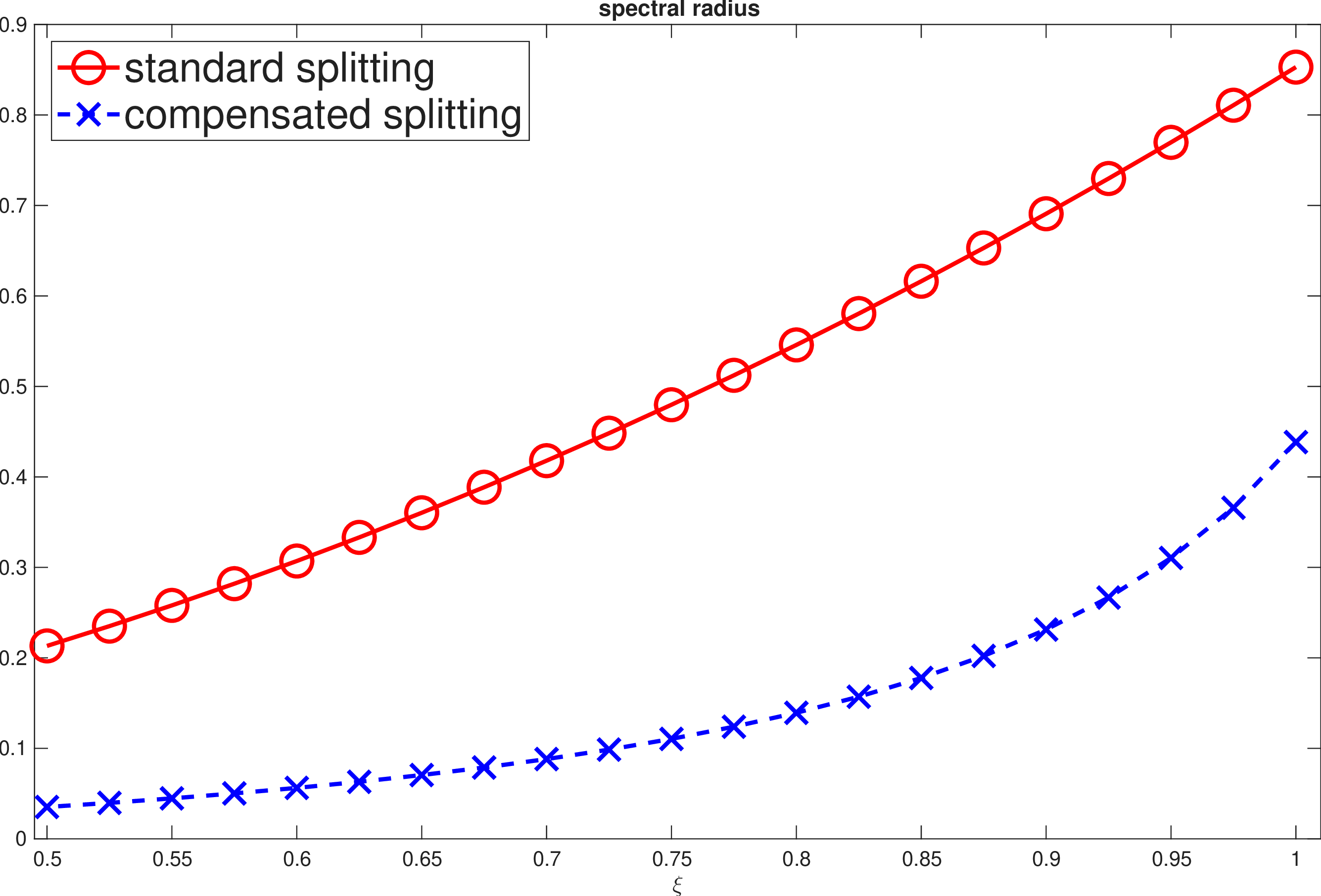
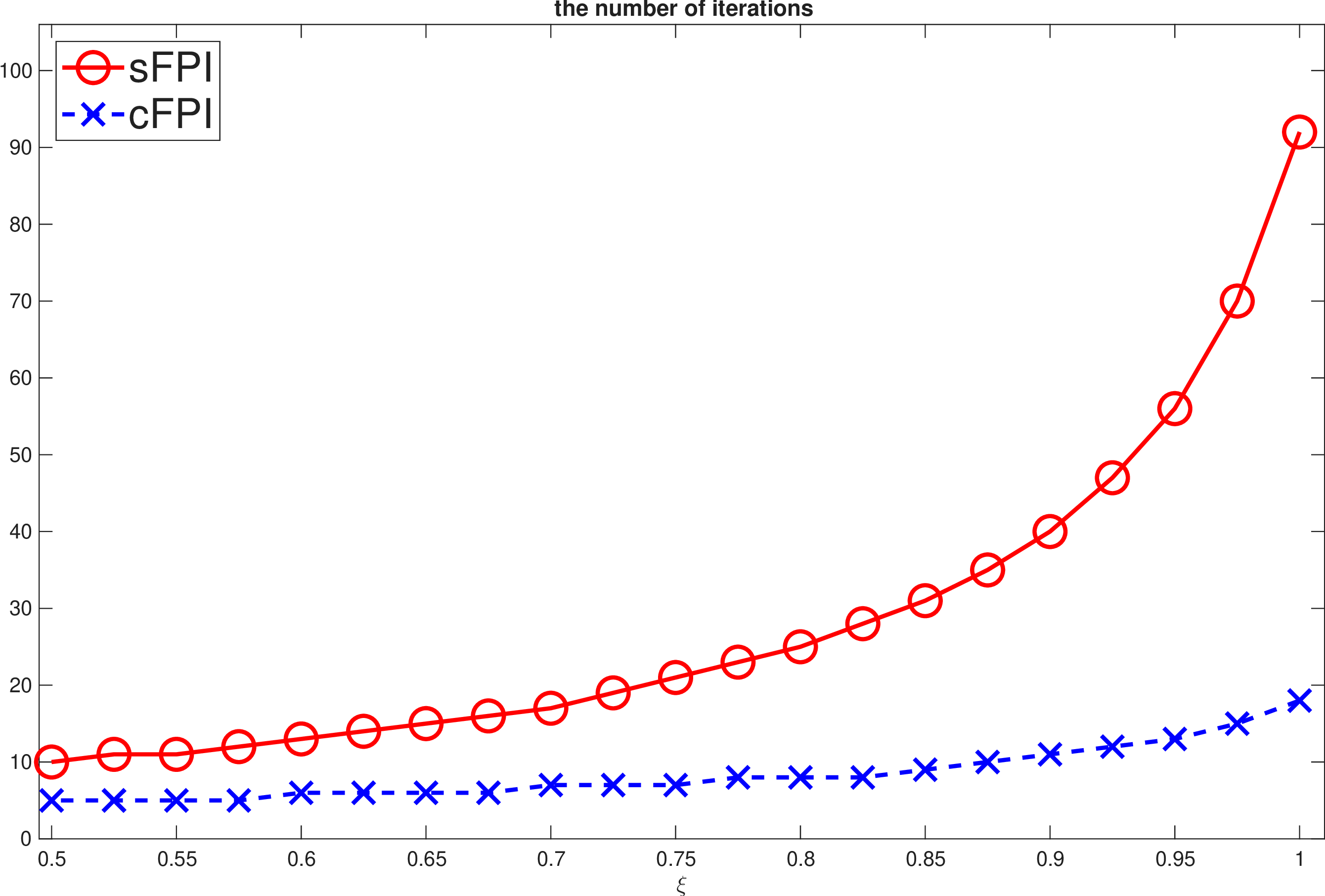
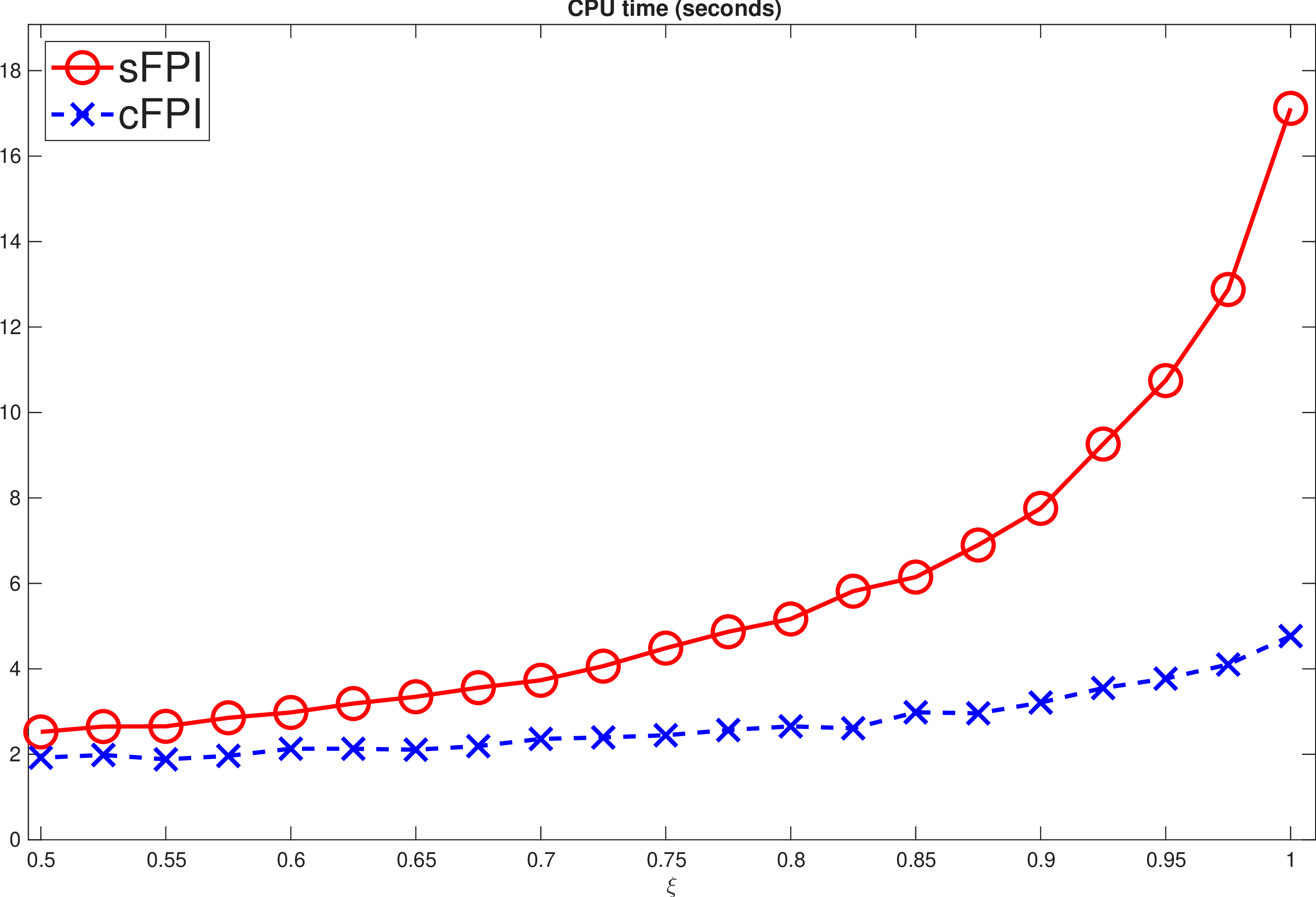
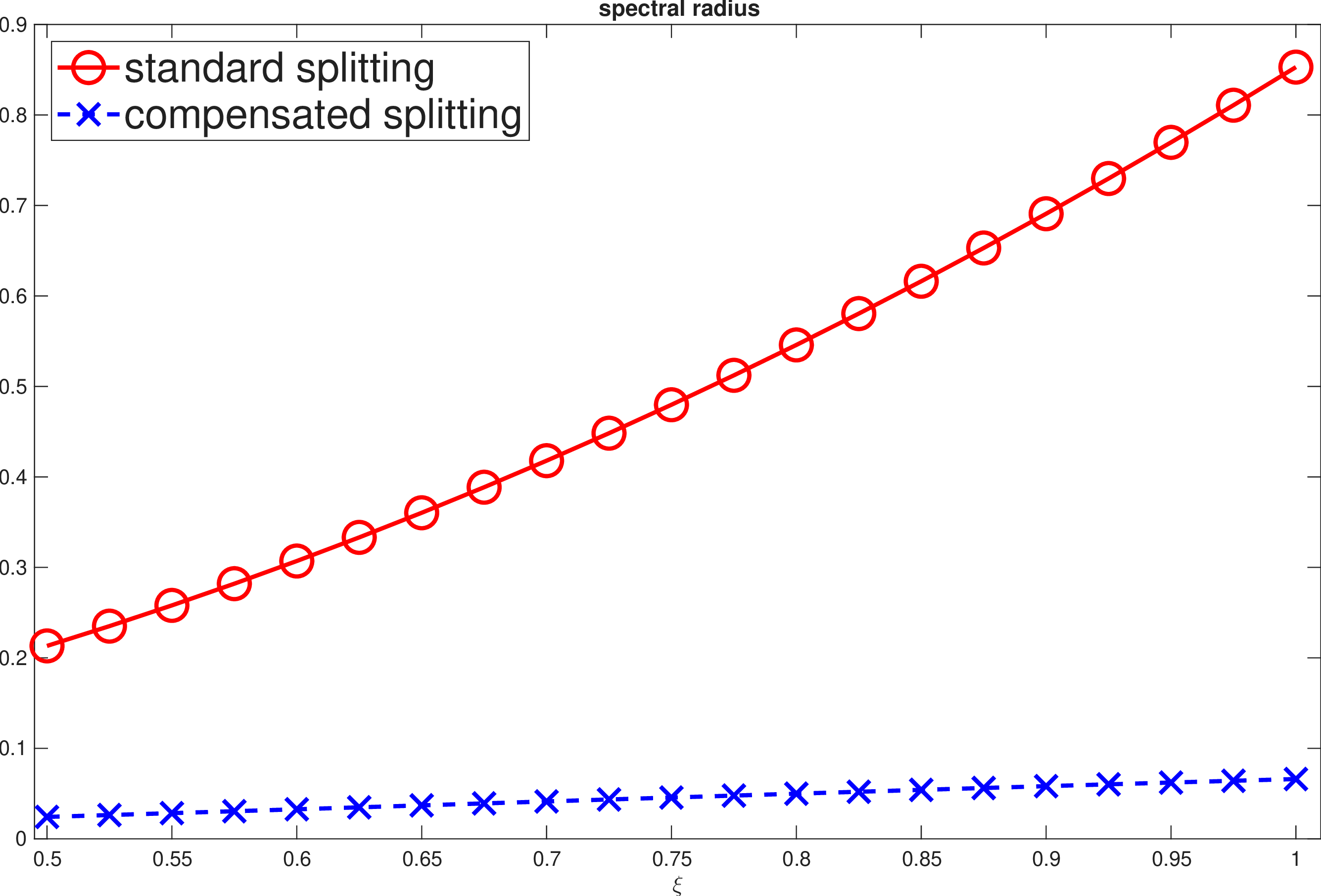
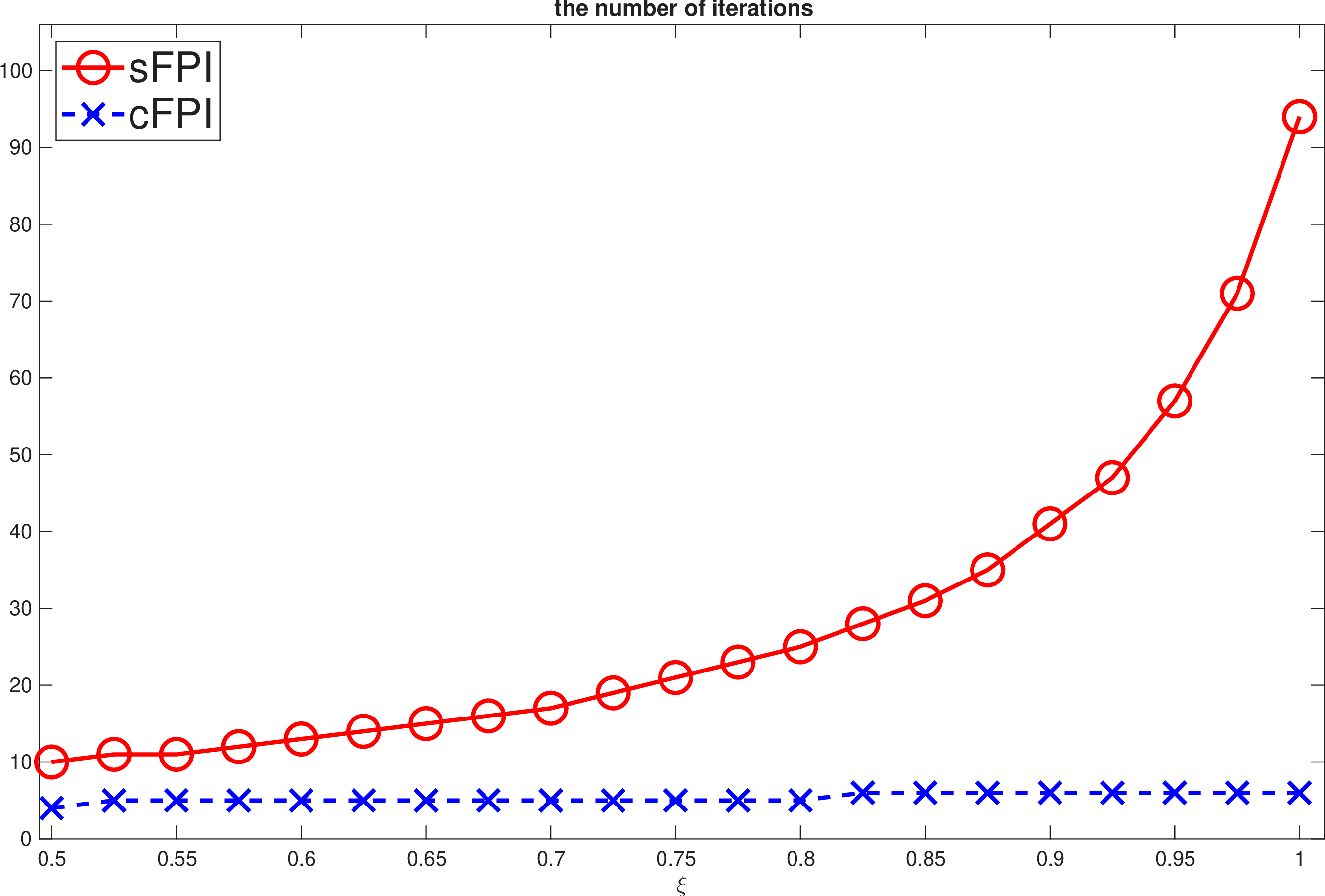
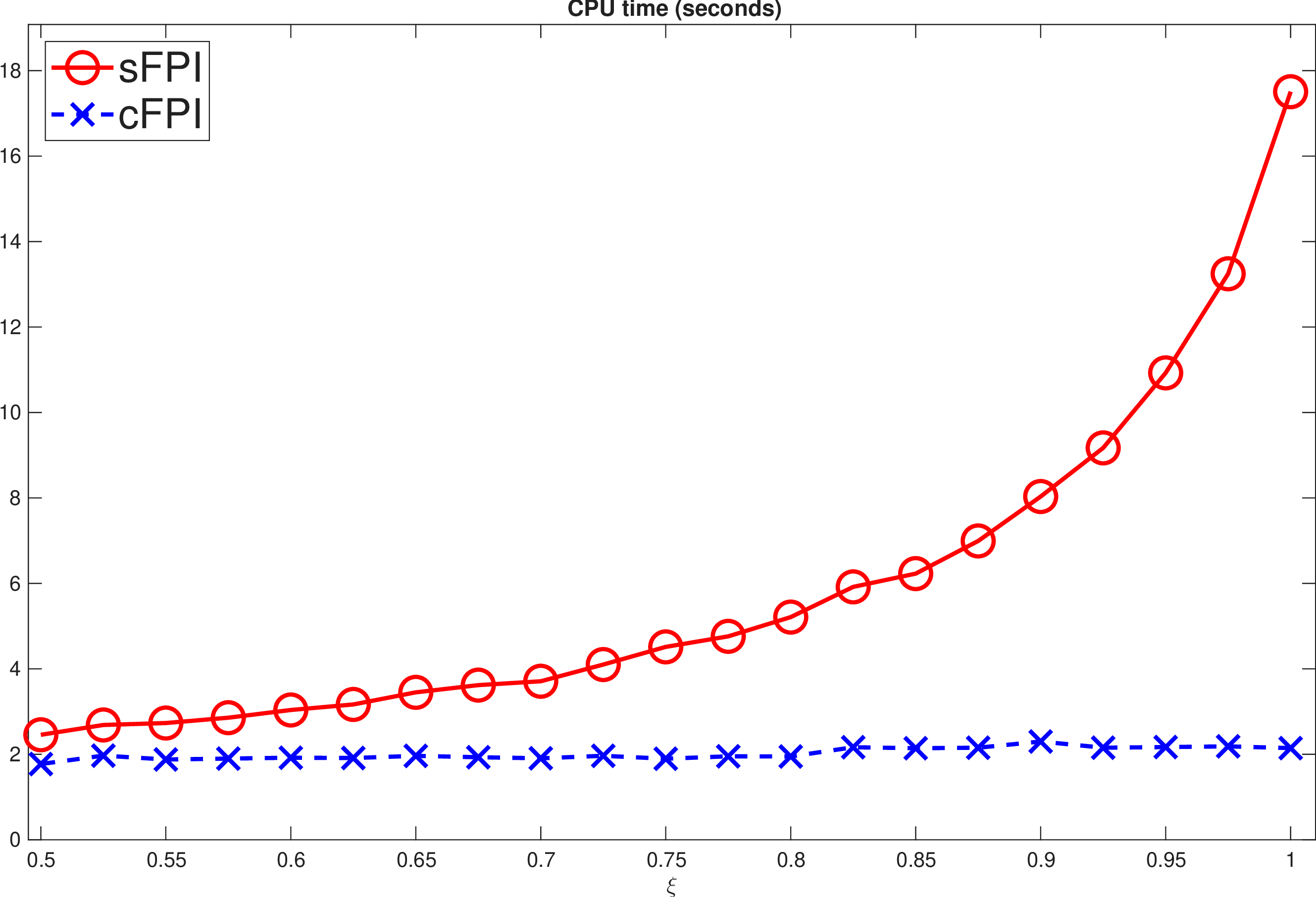
Figure 2: Numerical performance on Example 1 with the first row for \(A=A_0\) and the second row for \(A=-A_0\), as \(\xi\) varies in \([0.5,1]\)..
Example 1.
The matrix \(A\) is the well-known matrix as in HEAT1 [1]. We take \(\ell=40\) and define the mesh size \(h = 1/(\ell+1)\), and let \(\pmb{e}_1, \pmb{e}_{\ell}\in\mathbb{R}^{\ell}\) be the first and last columns of \(I_{\ell}\), respectively, and \[K =
\left[\begin{array}{ccccc}
2 & -1 & & & \\
-1 & 2 & -1 & & \\
& \ddots & \ddots & \ddots & \\
& & -1 & 2 & -1 \\
& & & -1 & 2
\end{array}\right]\in\mathbb{R}^{\ell\times \ell}, \quad
C =
\left[\begin{array}{ccccc}
0 & 1 & & & \\
-1 & 0 & 1 & & \\
& \ddots & \ddots & \ddots & \\
& & -1 & 0 & 1 \\
& & & -1 & 0
\end{array}\right]\in\mathbb{R}^{\ell\times \ell},\] \(E_1 = \pmb{e}_1\pmb{e}_1^{\mathop{\mathrm{T}}}\), \(E_{\ell} = \pmb{e}_{\ell} \pmb{e}_{\ell}^{\mathop{\mathrm{T}}}\). We
construct \(A_0\) as \[\label{eg3:eq1}
A_0 = \frac{-(I_{\ell}\otimes K + K\otimes I_{\ell})+0.5(E_1\otimes I_{\ell} + E_{\ell}\otimes I_{\ell})}{h^2} + \frac{I_{\ell}\otimes C}{2h} \in\mathbb{R}^{n\times n}\qquad{(2)}\] with \(n=\ell^2\). We take
\(B = \texttt{randn}(n,5)\), \(m=1\) and \[N_1=\xi
\begin{bmatrix}
7.8 & -1 & -0.05 & & \\
-1 & 7.8 & -1 & \ddots & \\
-0.05 & -1 & \ddots & \ddots & -0.05 \\ & \ddots & \ddots & \ddots & -1 \\ & & -0.05 & -1 & 7.8
\end{bmatrix},\] where \(\xi\) is a parameter varying from \(0.5\) to \(1\). Provably, \(\rho(\mathscr{M}^{-1}\mathscr{N})=c\xi^2\) where \(c>0\) is a constant independent of \(\xi\) and thus increases as \(\xi\)
does. This fact holds for the two other examples later.
We will solve two parameterized generalized Lyapunov equations 1 with \(A=\pm A_0\), respectively, with \(\ell=40\) yielding \(n=1600\). In 2, with respect to the standard splitting 3 and our compensated splitting 7 with 9 , we compare, as \(\xi\) varies, spectral radius, the number of iterations, and CPU in seconds, for the case \(A=A_0\) (frist row) and \(A=-A_0\) (second row). We have the following observations:
(a) For the range of \(\xi\in [0.5,1]\), both \(\rho(\mathscr{M}^{-1}\mathscr{N})\) and \(\rho(\widetilde{\mathscr{M}}^{-1}\widetilde{\mathscr{N}}\,)\) are less than \(1\), indicating both sFPI and the proposed cFPI are convergent.
(b) It makes no difference in the spectral radius \(\rho(\mathscr{M}^{-1}\mathscr{N})\) whether \(A=A_0\) or \(-A_0\). This is expected because the spectral radius is invariant with respect to \(A=\pm A_0\). But the story is entirely different for the compensated splitting. Besides \(\rho(\widetilde{\mathscr{M}}^{-1}\widetilde{\mathscr{N}}\,)\) is smaller than \(\rho(\mathscr{M}^{-1}\mathscr{N})\) at each \(\xi\) in both cases, \(\rho(\widetilde{\mathscr{M}}^{-1}\widetilde{\mathscr{N}}\,)\) for the case \(A=-A_0\) is much smaller than it for the case \(A=A_0\) at the same \(\xi\). The phenomenon can be quantitatively explained by our earlier discussion following 1, as the eigenvalues of \(A_0\) lie in the left-half plane.
(c) For the case \(A=-A_0\) whose eigenvalues lie in the right-half plane, \(\rho(\widetilde{\mathscr{M}}^{-1}\widetilde{\mathscr{N}}\,)\) increases very slowly as \(\xi\) increases and always stays below \(0.1\), while \(\rho(\mathscr{M}^{-1}\mathscr{N})\) grows at a much faster pace and ends up being \(0.85\) at \(\xi=1\). As a results, cFPI runs much faster than sFPI, respectively at each \(\xi\).


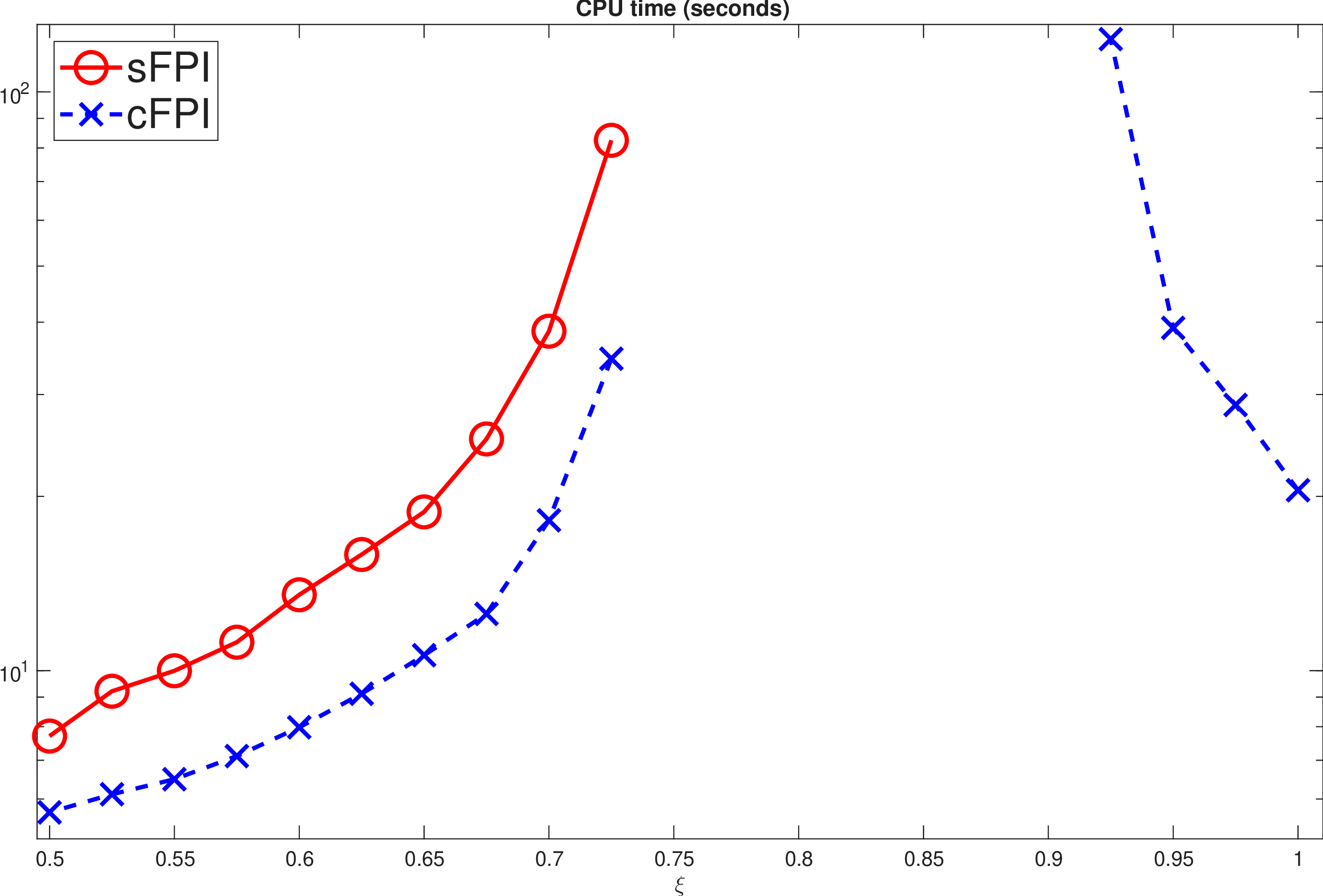
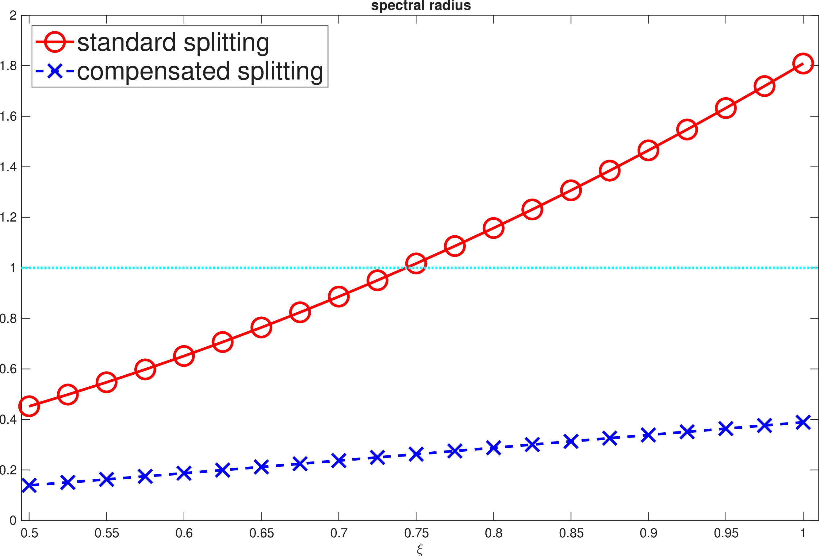
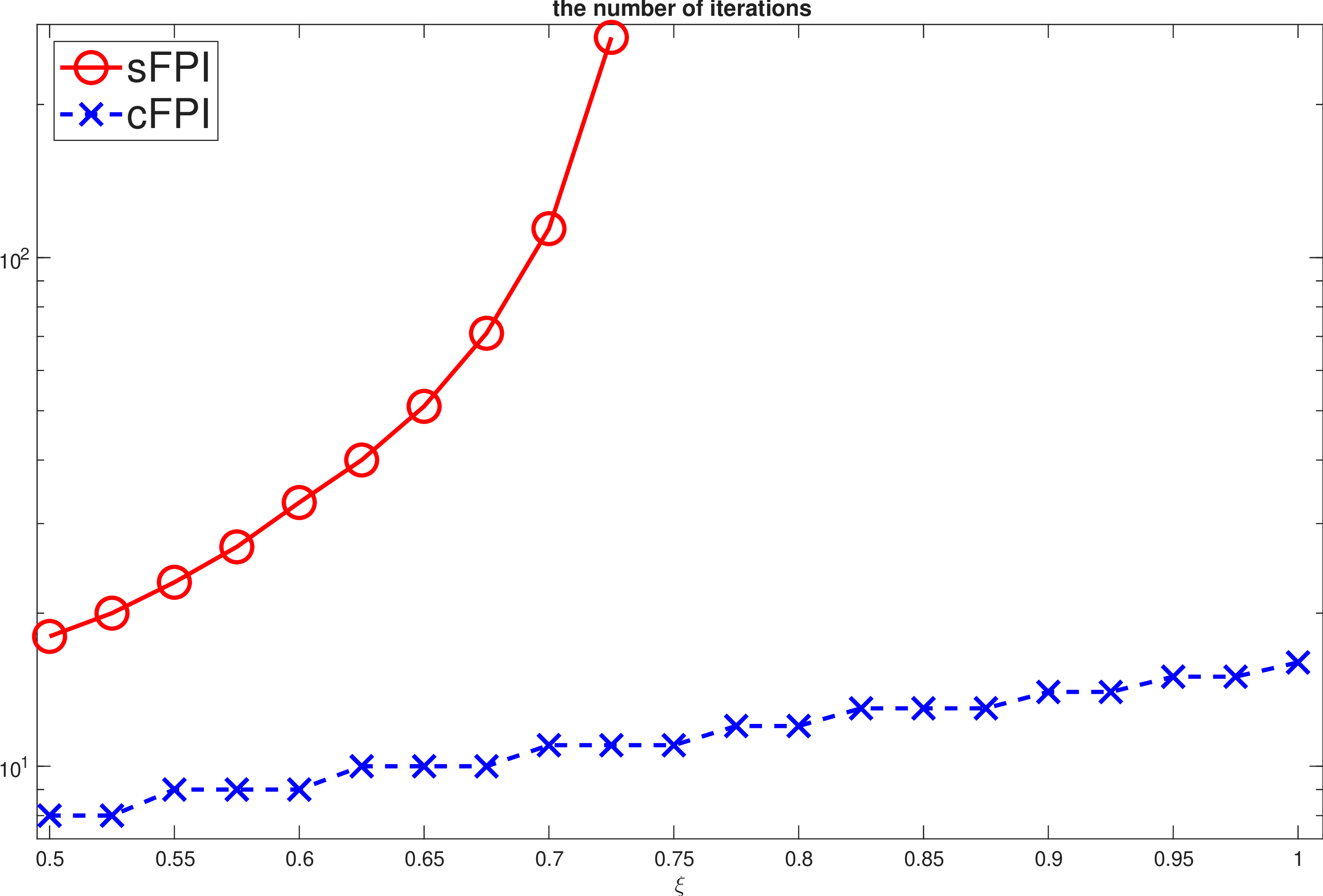
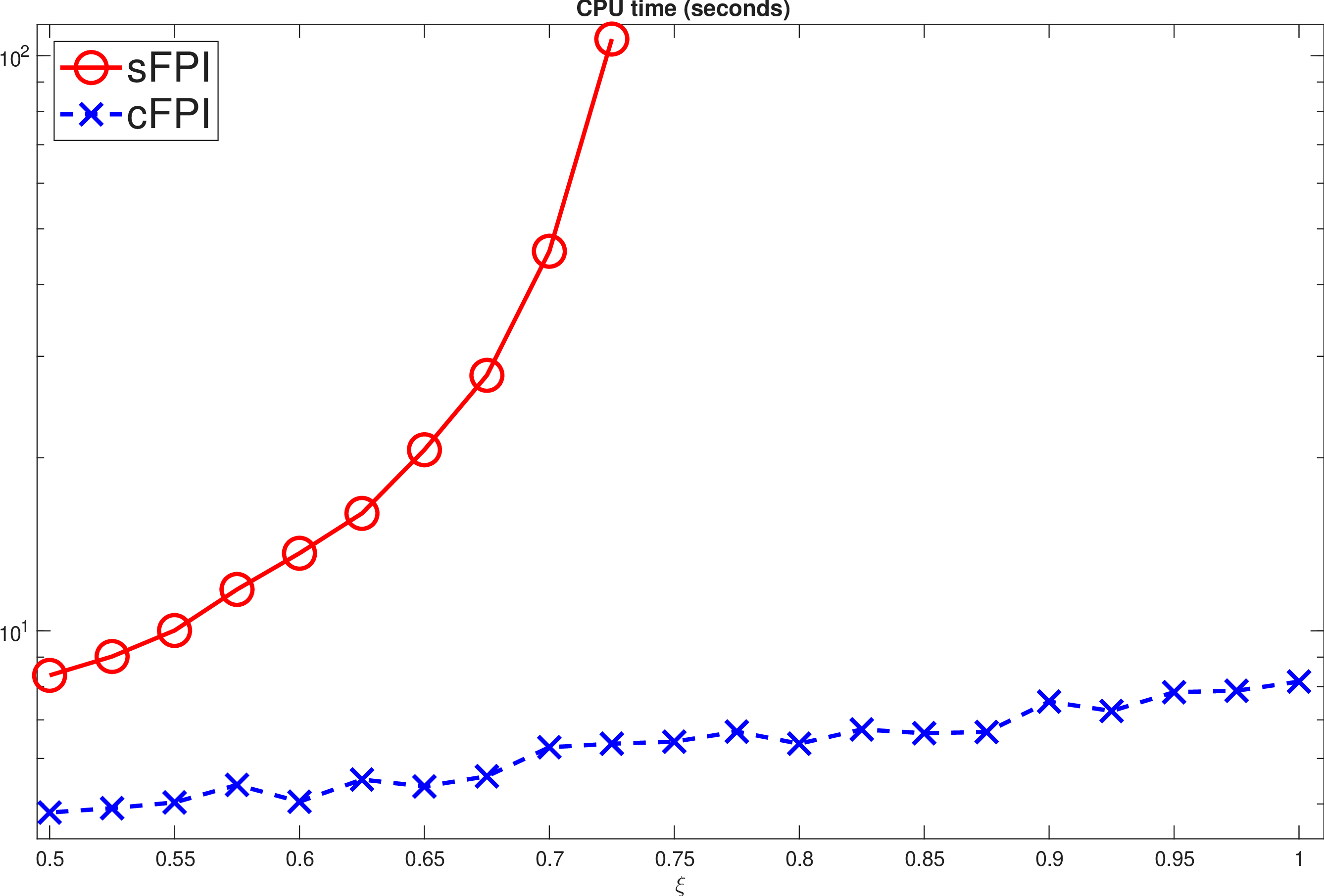
Figure 3: Numerical performance on Example 2 with the first row for \(A=A_0\) and the second row for \(A=-A_0\), as \(\xi\) varies in \([0.5,1]\). No numerical result is shown when the associated fixed-point iteration is deemed divergent..
Example 2.
The matrix \(A=\pm A_0\)with \(A_0\) being the tridiagonal matrix \[\label{eq:1-2-1} A_0 = \left[\begin{array}{ccccc} -2 & 1 & & & \\ 1 & -2 & 1 & & \\ & \ddots & \ddots & \ddots & \\ & & 1 & -2 & 1 \\ & & & 1 & -2 \end{array}\right]\in\mathbb{R}^{n\times n},\qquad{(3)}\] \(n=1000\), \(B=\texttt{randn}(n,2)\in\mathbb{R}^{n \times 2}\), \(m=5\), and \(N_j = 2\cdot 10^{-4}\times\xi\times C_jC_j^{\mathop{\mathrm{T}}}\) with each \(C_j=\texttt{randn}(n,10)\), where \(\xi\) is a parameter varying from \(.5\) to \(1\). Numerical results are shown in 3. We have the following observations:
(i) Provably \(\rho(\mathscr{M}^{-1}\mathscr{N})\) monotonically increases and it crosses \(1\) at \(\xi\) somewhere between \(0.725\) and \(0.75\). Because of that, sFPI converges for \(\xi\le 0.725\) and diverges otherwise.
(ii) Interestingly, for the case \(A=A_0\), \(\rho(\widetilde{\mathscr{M}}^{-1}\widetilde{\mathscr{N}}\,)\) shows a “pop-up” starting at \(\xi=0.75\) until \(\xi=0.9\). Excluding the period of the “pop-up”, it appears \(\rho(\widetilde{\mathscr{M}}^{-1}\widetilde{\mathscr{N}}\,)\) is less than \(\rho(\mathscr{M}^{-1}\mathscr{N})\). The sudden “pop-up” may be explained by our earlier discussion following 1: \(A_0\) is negative definite and its eigenvalues lie in the left-half plane, and \(E\) collectively moves the eigenvalues of \(A=A_0\) rightward towards \(0\), potentially crossing over to the right-side of \(0\).
(iii) Before \(\xi=0.75\) and after \(\xi=0.9\), \(\rho(\widetilde{\mathscr{M}}^{-1}\widetilde{\mathscr{N}}\,)\) is smaller than \(1\), and thus cFPI converges for \(\xi\) before \(0.75\) and after \(0.90\).
(iv) As in 1, for the case \(A=-A_0\), \(\rho(\widetilde{\mathscr{M}}^{-1}\widetilde{\mathscr{N}}\,)\) increases very slowly as \(\xi\) increases. It is noted that \(A=-A_0\) is positive definite and its eigenvalues lie in the right-half plane. Collectively, \(E\) moves the eigenvalues of \(A=A_0\) rightward further away from \(0\).
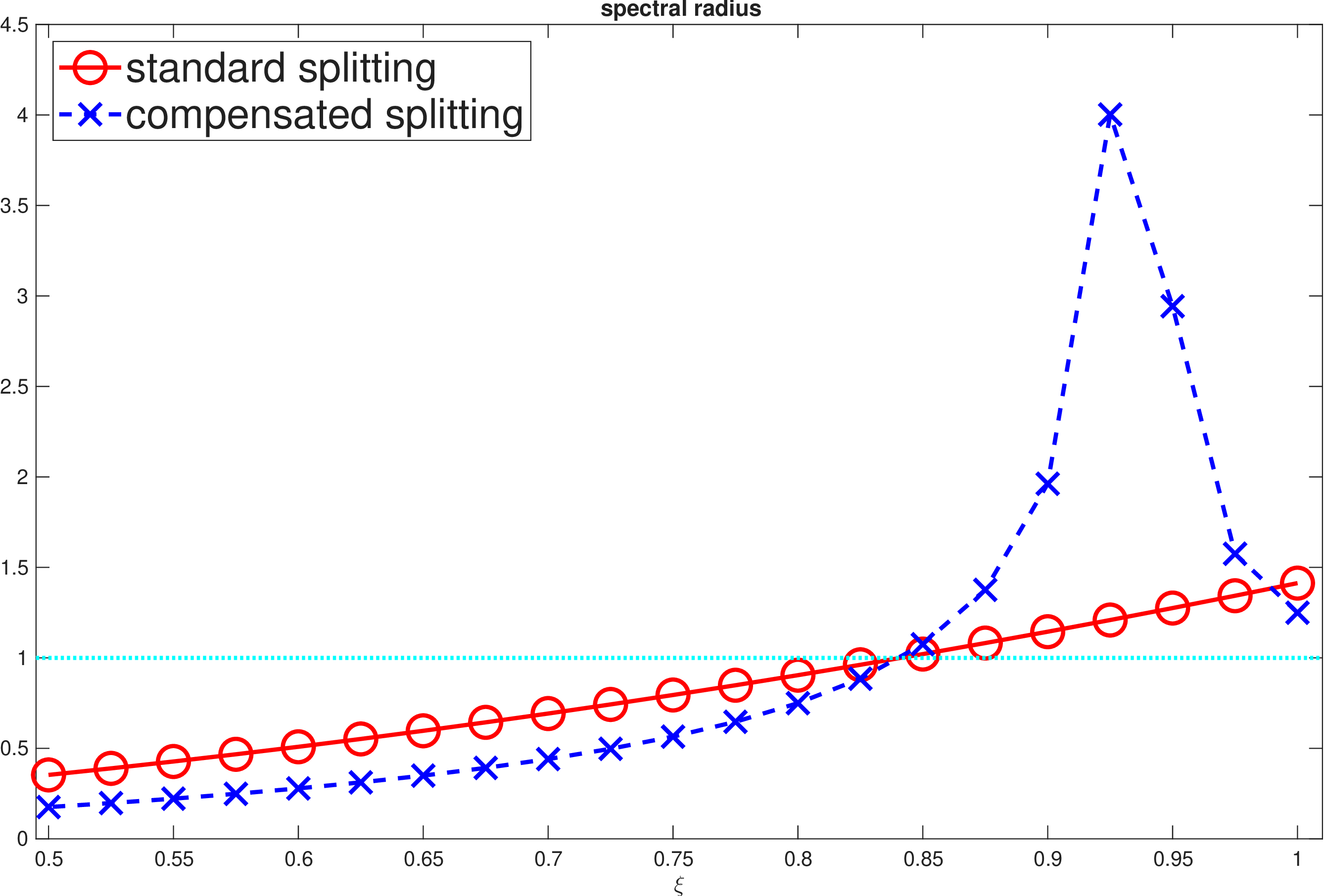
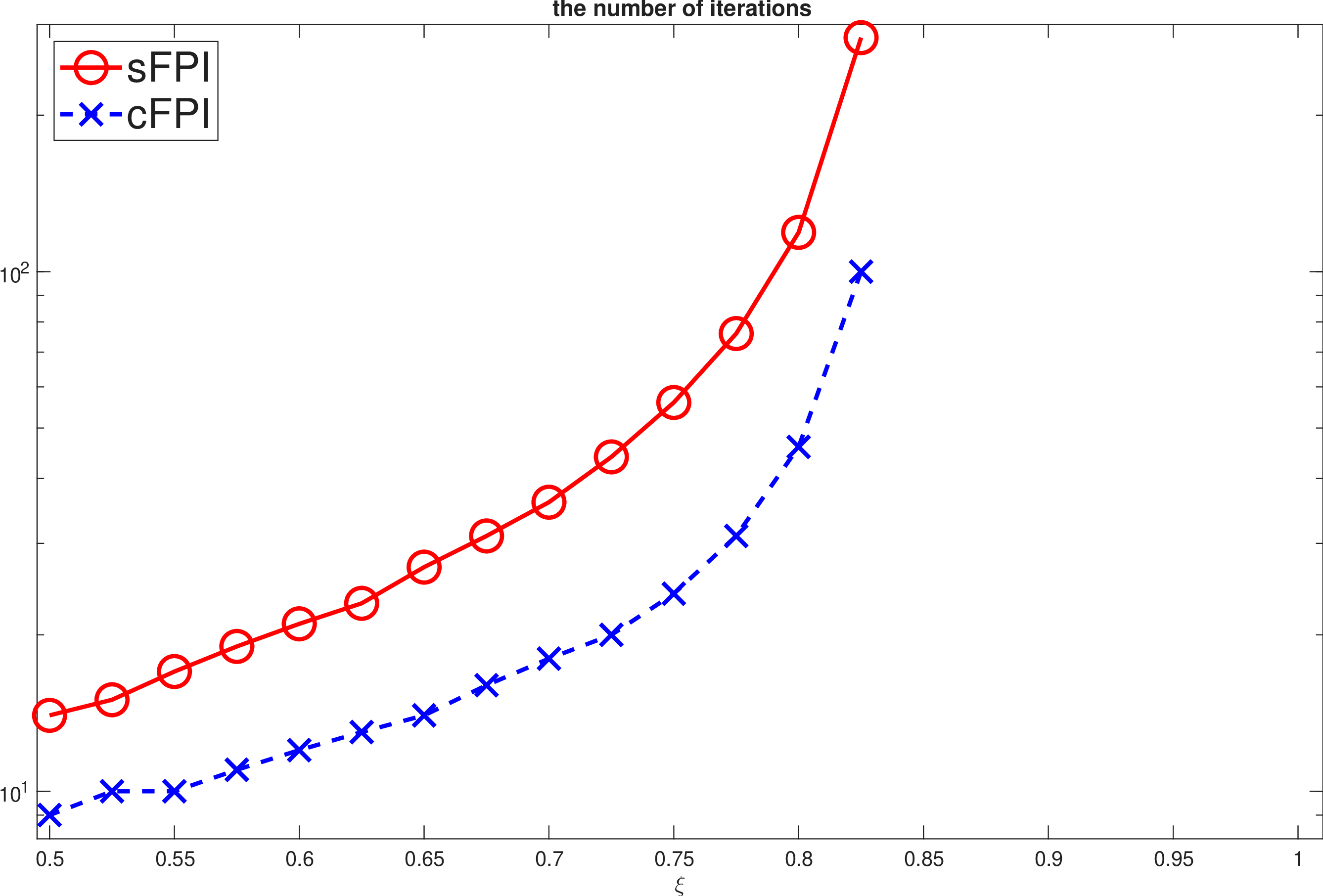
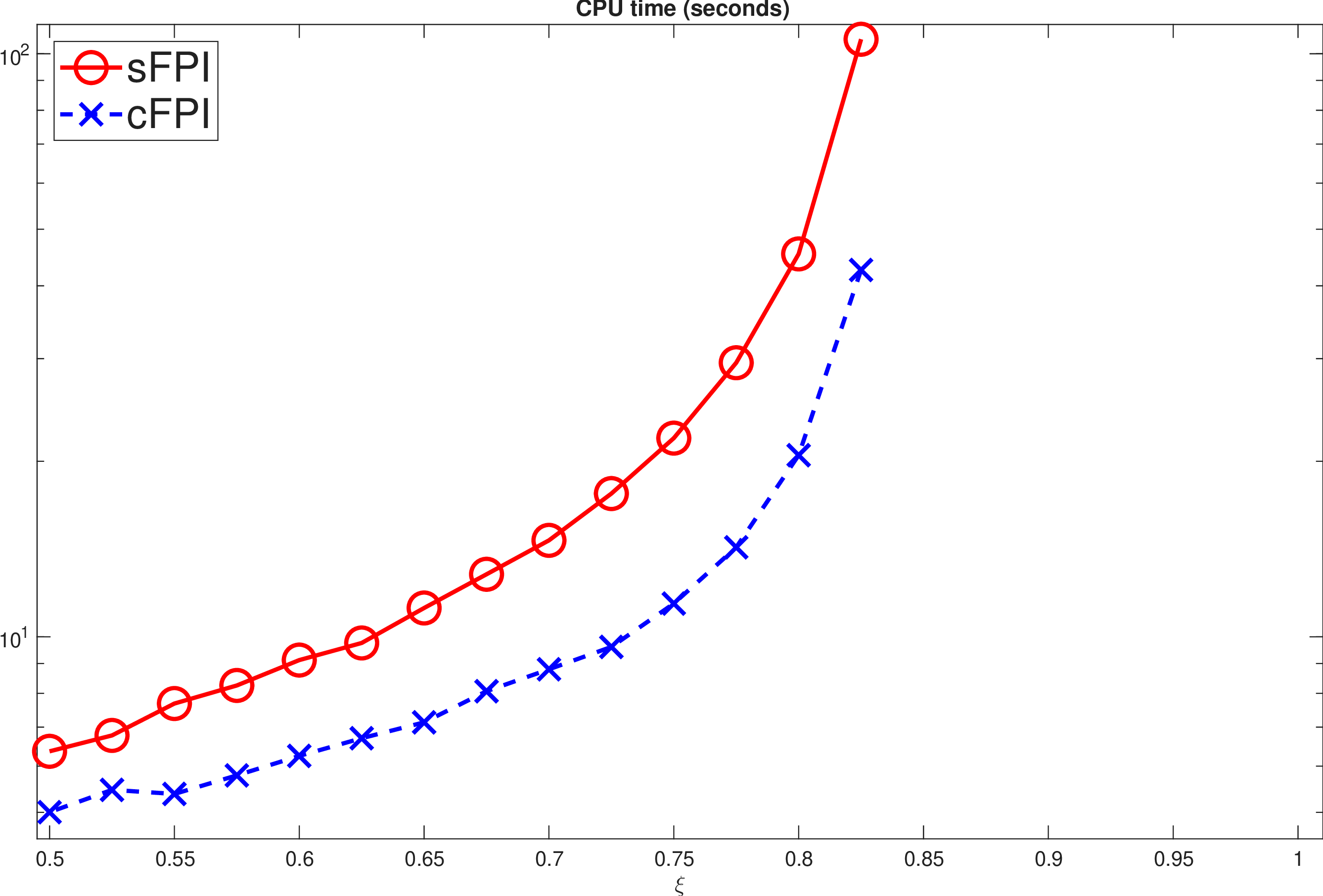
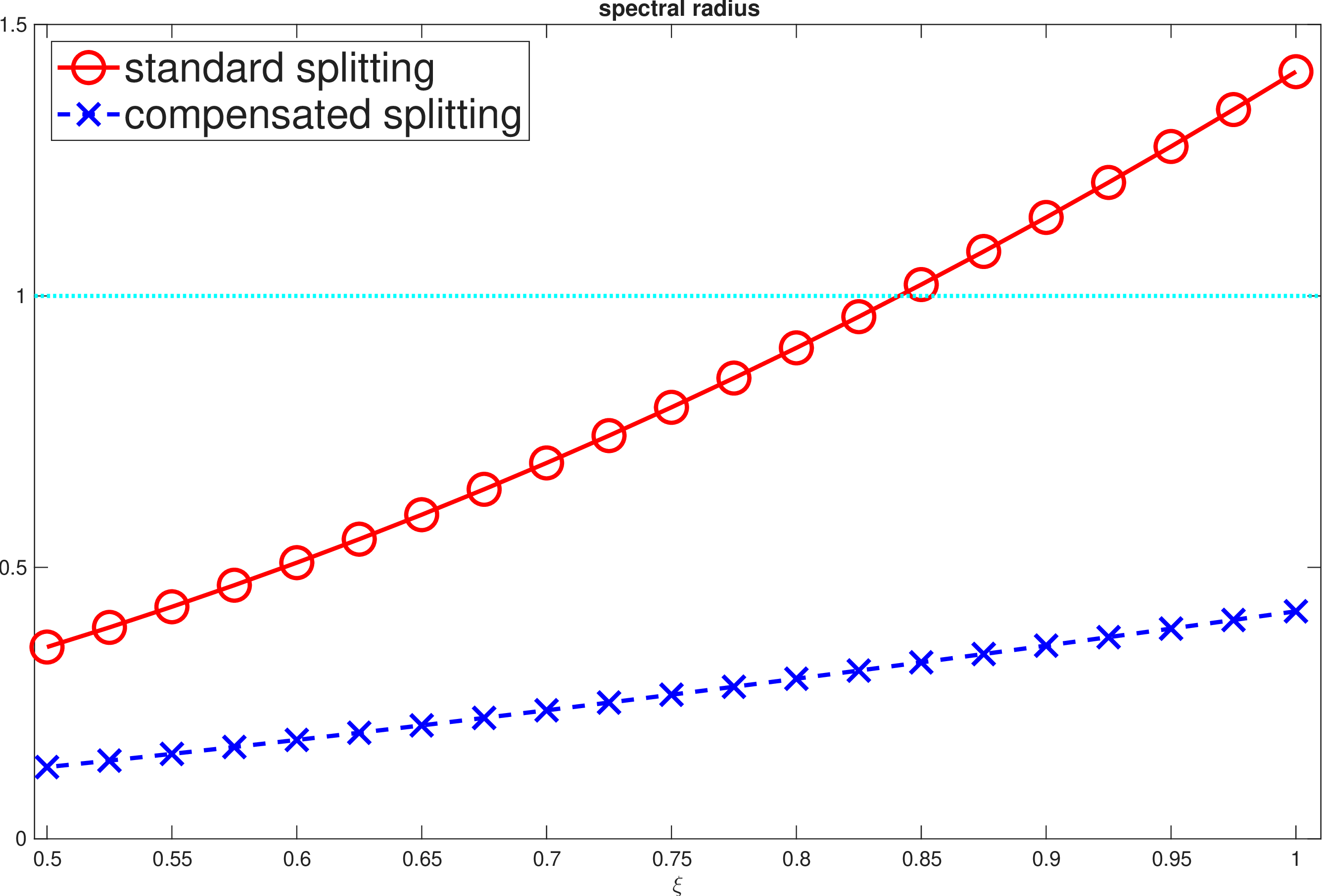
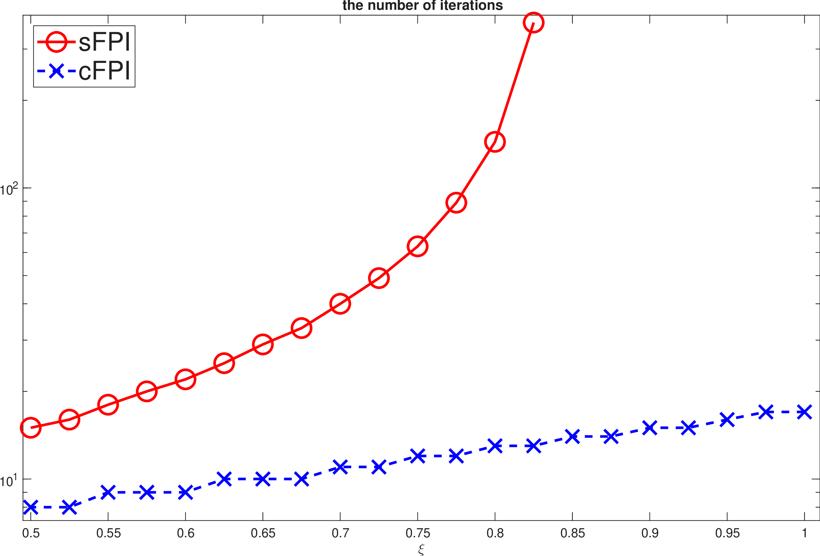
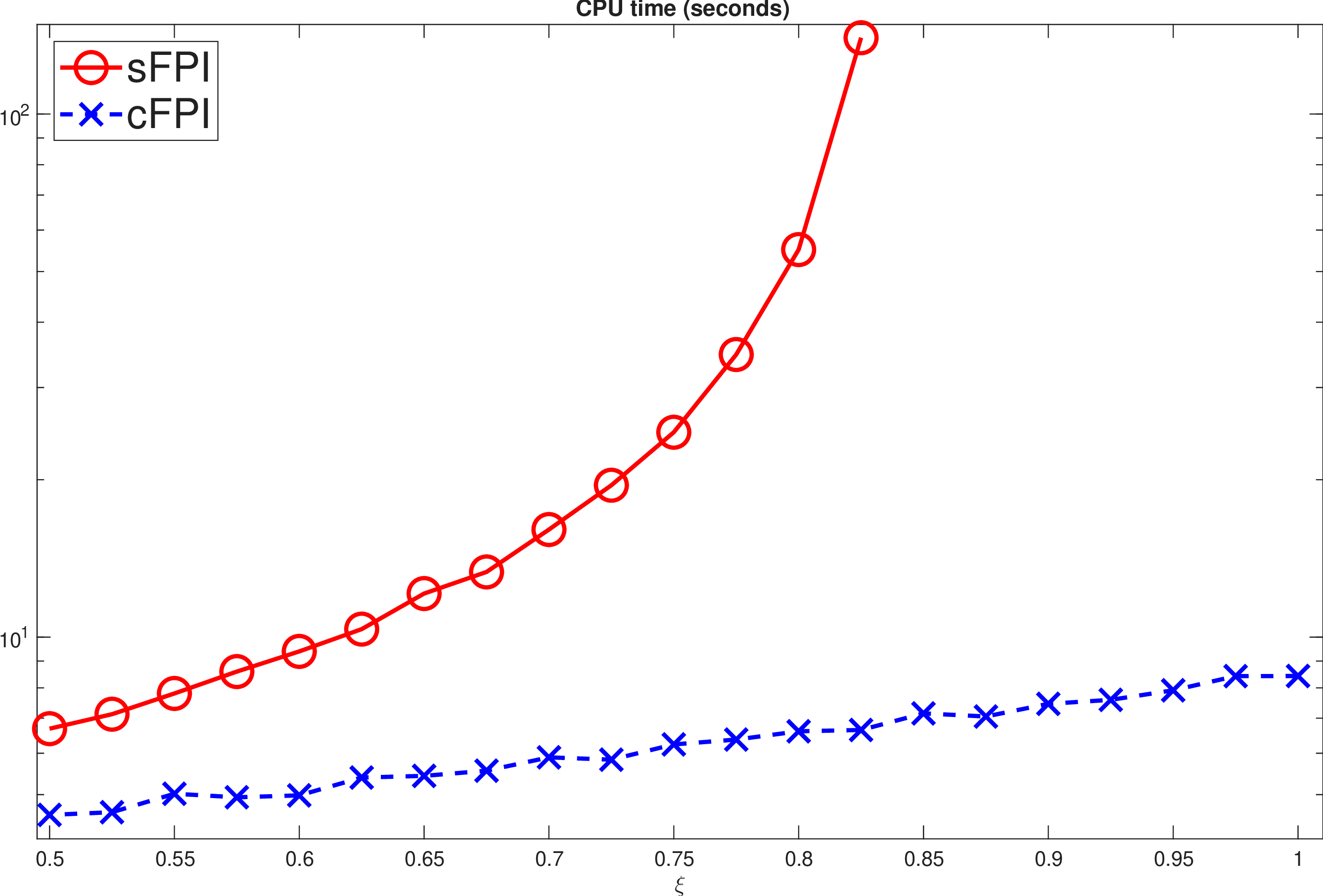
Figure 4: Numerical performance on Example 3 with the first row for \(A=A_0\) and the second row for \(A=-A_0\), as \(\xi\) varies in \([0.5,1]\). No numerical result is shown when the associated fixed-point iteration is deemed divergent..
Example 3.
This is a complex example. We add a small imaginary number to the diagonal of the one in ?? to get \[\label{eq:1-2-1:c} A_0= \left[\begin{array}{ccccc} -2 & 1 & & & \\ 1 & -2 & 1 & & \\ & \ddots & \ddots & \ddots & \\ & & 1 & -2 & 1 \\ & & & 1 & -2 \end{array}\right]+{\tt 1i}\times 10^{-8}\times I_n\in\mathbb{C}^{n\times n},\qquad{(4)}\] \(n=1000\), \(B=\texttt{randn}(n,2)+\texttt{1i*randn}(n,2)\), \(m=5\), and \(N_j = 2\cdot 10^{-4}\times\xi\times C_jC_j^{\mathop{\mathrm{H}}}\) with each \[C_j=\texttt{randn}(n,5)+\texttt{1i*randn}(n,5),\] where \(\xi\) is a parameter varying from \(.5\) to \(1\). Adding a small imaginary number in ?? is to ensure that calling the Schur decomposition of \(A\) at the beginning of sFPI yields a complex Schur form. This will equalize the computational complexity per fixed-point iterative steps in both sFPI and cFPI. Numerical results are shown in 4. We witness similar things to 3:
(1) Provably \(\rho(\mathscr{M}^{-1}\mathscr{N})\) monotonically increases and it crosses \(1\) at \(\xi\) somewhere between \(0.825\) and \(0.85\). Because of that, sFPI converges for \(\xi\le 0.825\) and diverges otherwise.
(2) For the case \(A=A_0\), \(\rho(\widetilde{\mathscr{M}}^{-1}\widetilde{\mathscr{N}}\,)\) shows a “pop-up” starting at \(\xi=0.85\) until likely some \(\xi>1\) if we let it go larger. Once again, the sudden “pop-up” may be explained by our earlier discussion following 1, as the eigenvalues of \(A=A_0\) lie in the left-half plane.
(3) As in the previous two examples, for the case \(A=-A_0\), \(\rho(\widetilde{\mathscr{M}}^{-1}\widetilde{\mathscr{N}}\,)\) increases very slowly as \(\xi\) increases. It is verified numerically that \(A=-A_0\) has its eigenvalues lying in the right-half plane.
4 Concluding Remarks↩︎
The generalized Lyapunov equation \[AX + XA^{\mathop{\mathrm{H}}} + \sum_{j=1}^{m}N_j X N_j^{\mathop{\mathrm{H}}} + BB^{\mathop{\mathrm{H}}} = 0\] arises frequently in applications. Such an equation is naturally split into \(\mathscr{M}(X)=\mathscr{N}(X)-BB^{\mathop{\mathrm{H}}}\) where \(\mathscr{M}(X)=AX + XA^{\mathop{\mathrm{H}}}\) and \(\mathscr{N}(X)=\sum_{j=1}^{m}N_j X N_j^{\mathop{\mathrm{H}}}\), and it has been done frequently to yield the commonly used standard fixed-pointed iteration (sFPI) for solving the equation. The iteration converges if the spectral radius \(\rho(\mathscr{M}^{-1}\mathscr{N})<1\) but otherwise diverges in general. In this paper, we propose a compensated splitting technique to tackle situations where \(\rho(\mathscr{M}^{-1}\mathscr{N})\ge 1\) or \(\rho(\mathscr{M}^{-1}\mathscr{N})<1\) but too close to \(1\) leading very slow convergence. The basic idea is to compensate \(\mathscr{M}(X)\) by projecting \(\mathscr{N}(X)\) into an operator in the form \(EX + XE^{\mathop{\mathrm{H}}}\) to merge with \(\mathscr{M}(X)\), yielding the so-called compensated splitting \(\widetilde{\mathscr{M}}(X)=\widetilde{\mathscr{N}}(X)-BB^{\mathop{\mathrm{H}}}\) for which there is a corresponding fixed-point iteration called the compensated fixed-pointed iteration (cFPI). Ideally, we should minimize \(\rho(\widetilde{\mathscr{M}}^{-1}\widetilde{\mathscr{N}}\,)\) over matrix \(E\), but that is not practical. Instead we determine \(E\) by 12 . It is shown that 12 has a unique global minimizer in the real case and a unique global minimizer with the smallest Frobenius norm in the complex case. Compactly the optimal \(E\) is given by \[E=\frac{1}{n(1+\mu)}\sum_{j=1}^m\mathop{\mathrm{tr}}(\bar{N}_{j})\left[N_j -\frac{1}{2n} \mathop{\mathrm{tr}}(N_{j})\cdot I_n\right],\] where \(\mu\ge 0\) is a regularizing parameter to control the magnitude of \(E\). At this point, we have little idea on how to determine a good \(\mu\), and in fact in our reported numerical experiments in 3, we simply take \(\mu=0\) as the default.
Unfortunately, our current 12 to determine \(E\) does not involve the \(\mathscr{M}\)-part in any way. Quantitatively, we have analyse the interaction between this optimal \(E\) and the \(\mathscr{M}\)-part. Our numerical experiments appear to behave consistently with our analysis, while demonstrating superiority of cFPI to sFPI.
In our numerical experiments, we limit the problem sizes, i.e., \(n\), modest so that involved Lyapunov equations in the middle of computations can be solved by the Bartels-Stewart method [14] with ease on everyday personal computers. For that reason, our purpose in this paper is two-fold: one is to demonstrate our compensated splitting can rescue the natural splitting, the commonly used one 3 when the resulting sFPI 4 diverges, and the other one is to show that the compensated splitting can speed up cFPI when it indeed converges. It is expected the key idea in this paper can be combined with more sophisticated subspace-based projection iterative methods, e.g., [12], [13], to yield more efficient methods for large scale generalized Lyapunov equations. Such investigations will be forthcoming.
A similar looking to the generalized Lyapunov equation is the generalized Sylvester equation \[AX + XB^{\mathop{\mathrm{H}}} + \sum_{j=1}^{m}N_j X M_j^{\mathop{\mathrm{H}}} + C = 0.\] It arises from, for example, discretizing certain partial differential equations [16] and perhaps other places, and it too possesses a natural splitting that leads to a natural fixed-point iteration, similarly to the discussions we had in 1 for the generalized Lyapunov equation. Due to high similarity, our compensated splitting in 2 can be straightforwardly attempted for potential improvement. We will leave the detail to another paper.
References↩︎
Department of Mathematics, Nanchang University, 999 Xuefu Road, Nanchang, Jiangxi, 330031, China. Supported by the National Natural Science Foundation of China under grant No. 12371379 and No. 12361080, and Jiangxi Provincial Natural Science Foundation under grant No. 20224BAB211006. Email:
chenhongjia@ncu.edu.cn.↩︎Department of Mathematics, University of Texas at Arlington, Arlington, TX 76019-0408, USA. Supported in part by NSF DMS-2407692. Email:
rcli@uta.edu.↩︎