Local-to-Global Exactness of SDP Relaxations
for Sparse QCQPs
January 01, 1970
Abstract
We study exact semidefinite programming (SDP) relaxation for a given sparse quadratically constrained quadratic program (QCQP). The SDP relaxation is exact if, whenever it has an optimal solution, it admits a rank-at-most-one optimal solution that corresponds to an optimal solution of the QCQP. Using the maximal cliques of a chordal extension of the aggregate sparsity pattern graph of the data matrices, we formulate the SDP relaxation in terms of clique-wise matrix variables and develop a local-to-global framework for certifying exactness. For each clique-wise matrix variable, we introduce a local sub-SDP with two parameters: a local right-hand-side vector and a consistency matrix specifying the values of entries shared by overlapping clique-wise matrix variables. In the main theorem, these parameters are determined by an optimal solution of the global clique-wise SDP. The theorem shows that if the resulting local sub-SDPs are exact, then the original SDP relaxation is exact. Under the additional assumption that any two distinct cliques intersect in at most one node, we present three classes of local QCQPs that can be incorporated into this framework: convex local QCQPs, local QCQPs characterized by sign-pattern conditions, and separable local QCQPs with a limited number of constraints. Examples illustrate how these different local QCQP classes can be combined in sparse QCQPs.
Key words. quadratically constrained quadratic program, semidefinite programming relaxation, exact SDP relaxation, sparse optimization, chordal graph, clique-wise formulation, local-to-global exactness, block-clique sparsity, rank-at-most-one optimal solution.
AMS Classification. 90C20, 90C22, 90C25, 90C26.
1 Introduction↩︎
Quadratically constrained quadratic programs (QCQPs) form a broad class of nonconvex optimization problems. They include many fundamental models in operations research, control, signal processing, and combinatorial optimization. A standard approach to such problems is to lift the quadratic terms to a symmetric matrix variable and to relax the resulting rank-at-most-one constraint, thereby obtaining a semidefinite programming (SDP) relaxation. SDP relaxations of QCQPs have been extensively studied; see, for example, [1]–[5] and the references therein. A central question is when such an SDP relaxation is exact, in the sense that it admits a rank-at-most-one optimal solution, which corresponds to an optimal solution of the original QCQP. (We refer to an optimal solution of rank at most one as a rank-at-most-one optimal solution.)
The exactness of SDP relaxations has been studied from several different viewpoints. One line of work derives exactness conditions directly in terms of the data matrices, including convexity [2] and sign-pattern conditions [6], [7]. Another line is based on the number of quadratic constraints and theoretical rank bounds for SDP solutions [4], [8], [9]. A further line studies exactness through geometric properties of the feasible region or of associated cones, such as non-intersecting quadratic constraints (NIQC) conditions [10]–[12] and the rank-one-generated (ROG) property [13]–[15]. The NIQC and ROG viewpoints are closely related, as discussed in [10], but they are qualitatively different in nature from coefficient-wise or constraint-count conditions: they depend on how the quadratic inequalities jointly shape the feasible region.
This paper develops a local-to-global exactness framework for sparse QCQPs that can be verified locally and then assembled into a global exactness certificate. Many existing exactness results are formulated for a single QCQP with a specific global structure as mentioned above. In sparse problems, however, different parts of the problem may have different structures: one part may correspond to a convex subproblem, another to a sign-pattern class, and another to a separable problem with a limited number of constraints. Convexity and sign-pattern conditions are particularly well suited to such a local treatment, because their exactness guarantees are stable under changes in local right-hand-side values and in the values shared by overlapping local subproblems. Rank-bound arguments based on the limited number of constraints can also be incorporated, although their applicability may depend on the parameters induced by the global problem. Since the ROG and NIQC viewpoints are more global and geometric in nature, they fall outside the scope of the present work.
Sparsity has long played an important role in semidefinite programming. For SDPs whose data matrices have a sparse aggregate pattern, chordal extensions and positive semidefinite matrix completion enable the replacement of a single large positive semidefinite constraint with smaller positive semidefinite constraints on maximal cliques [16]–[18]. The resulting clique-wise SDP is equivalent to the original SDP relaxation, but it is formulated in terms of local matrix variables linked by consistency constraints on overlaps. We adopt this clique-wise formulation for the analysis of exactness. We emphasize that the clique-wise formulation is used here as a theoretical tool for certifying exactness, rather than as a computational strategy for solving the sparse SDP relaxation. Once exactness has been certified, the SDP relaxation may be solved by any suitable SDP method. For computational methods for sparse SDPs based on chordal decomposition, see [17], [18].
The main contribution of this paper is the local-to-global exactness framework for sparse QCQPs. For a chordal extension of the aggregate sparsity pattern graph, we introduce a clique-wise SDP formulation and local sub-SDPs associated with the maximal cliques. Each local sub-SDP depends on a pair of parameters: a local right-hand-side vector \(\boldsymbol{\delta}\) and a consistency matrix \(\boldsymbol{U}\), which specifies the values of entries shared by local matrix variables. In the main theorem, these parameters are induced by an optimal solution of the global clique-wise SDP. The theorem shows how these induced local certificates can be assembled: if each local sub-SDP with its induced parameters \((\boldsymbol{\delta},\boldsymbol{U})\) admits a rank-at-most-one optimal solution, then the original SDP relaxation admits a rank-at-most-one optimal solution, and hence is exact. This ‘local-to-global exactness’ is established for general chordal extensions.
The remaining difficulty is ensuring consistency of local rank-at-most-one solutions on overlaps. For a general chordal extension, two maximal cliques may share more than one node. The resulting consistency constraints may then include off-diagonal entries of local matrix variables, and local rank-at-most-one solutions must satisfy nontrivial product relations on those overlapping off-diagonal entries. These relations are difficult to verify from local exactness alone. Therefore, when applying this framework, we impose a block-clique assumption: any two maximal cliques intersect in at most one node. Under this assumption all consistency constraints are diagonal, and consistency on overlaps reduces to matching squared scalar values. This permits the combination of local exactness mechanisms without imposing additional off-diagonal rank-one consistency conditions.
Under the block-clique assumption, the exactness mechanisms discussed above are recast as local results. Some are independent of the induced parameters \((\boldsymbol{\delta},\boldsymbol{U})\), while others, especially those based on rank bounds for separable subproblems, depend on them. We further prove a preservation result showing that certain dependent inequality constraints can be added without destroying local exactness. These results provide the local building blocks for the local-to-global exactness certification.
The theoretical significance of the local-to-global exactness framework lies in treating sparsity as part of the exactness analysis. The clique-wise formulation relates global rank-at-most-one attainment to local rank-at-most-one attainment. This provides a route to proving exactness of SDP relaxations of sparse QCQPs in settings where no single global exactness criterion applies to the entire problem. In this sense, the contribution is structural: it shows how sparsity can serve as a mechanism for certifying exact SDP relaxations. The examples in Section 5 illustrate how local exactness certificates can be assigned to different parts of the sparse structure and then assembled through diagonal consistency constraints.
We also mention two related lines of work. First, block-clique graph structures have appeared in doubly nonnegative (DNN) and completely positive (CPP) reformulations of quadratic optimization problems [15]. Although those works concern DNN and CPP reformulations rather than SDP exactness studied here, their use of block-clique structures is closely related to the block-clique assumption mentioned above.
Second, the present framework is complementary to extension results that preserve exact SDP relaxations under the addition of constraints on a fixed variable space [19]. These results may be viewed as a vertical extension of a QCQP, whereas the local-to-global exactness framework developed here gives a horizontal extension: exact sub-QCQPs on different variable subsets are combined through diagonal consistency constraints. A preliminary version of this horizontal viewpoint for separable QCQPs appeared in [20]; the present paper develops a more general sparse framework that combines several local exactness mechanisms through clique-wise decompositions.
The paper is organized as follows. Section 2 formulates the QCQP and its SDP relaxation, introduces the aggregate sparsity pattern graph, and derives the clique-wise formulation based on a chordal extension of the graph. Section 3 develops the local-to-global exactness framework. In particular, it introduces the local sub-SDPs associated with the clique-wise formulation developed in Section 2, proves the main theorem, and explains the role of diagonal consistency under the block-clique assumption. Section 4 establishes local exactness results for the three classes of sub-QCQPs used in the framework: convex sub-QCQPs, sub-QCQPs satisfying sign-pattern conditions, and separable sub-QCQPs with a limited number of constraints. It also presents a preservation result for dependent inequality constraints. Section 5 gives examples illustrating how these local exactness results can be combined in sparse QCQPs. Section 6 concludes the paper.
2 QCQP, SDP relaxation, and clique-wise reformulation↩︎
Let \(\mathbb{R}^n\) be the \(n\)-dimensional Euclidean space of column vectors \(\boldsymbol{x}= (x_1,\ldots,x_n)\), and \(\boldsymbol{x}^T\) the transposed row vector of each \(\boldsymbol{x}\in \mathbb{R}^n\). Let \(\mathbb{S}^n\) denote the linear space of \(n \times n\) symmetric matrices equipped with the inner product \(\langle\boldsymbol{A}, \, \boldsymbol{B}\rangle = \sum_{i=1}^n \sum_{j=1}^n [\boldsymbol{A}]_{ij} [\boldsymbol{B}]_{ij} \;\text{for } \boldsymbol{A}, \boldsymbol{B}\in \mathbb{S}^n,\) and let \(\mathbb{S}^n_+\) be the cone of \(n \times n\) symmetric positive semidefinite matrices. For \(\boldsymbol{A}\in \mathbb{S}^n\), we often write a quadratic form \(\boldsymbol{x}^T\boldsymbol{A}\boldsymbol{x}\) in \(\boldsymbol{x}\in \mathbb{R}^n\) as \(\langle\boldsymbol{A}, \, \boldsymbol{x}\boldsymbol{x}^T\rangle\).
2.1 QCQP and its SDP relaxation↩︎
Let \(\boldsymbol{A}_k \in \mathbb{S}^n\) \((k=0,1,\ldots,m)\) and \(\boldsymbol{b}\in \mathbb{R}^m\). We consider the following QCQP: \[\begin{align} \zeta & = & \inf \left\{ \langle\boldsymbol{A}_0, \, \boldsymbol{x}\boldsymbol{x}^T\rangle : \boldsymbol{x}\in \mathbb{R}^n, \; \langle\boldsymbol{A}_k, \, \boldsymbol{x}\boldsymbol{x}^T\rangle \trianglelefteq_k b_k \;(k=1,\ldots,m)\right\} \nonumber \\ & = & \inf \left\{ \langle\boldsymbol{A}_0, \, \boldsymbol{X}\rangle : \boldsymbol{X}\in \mathbb{S}^n_+, \;{\rm rank}(\boldsymbol{X}) \leq 1, \; \langle\boldsymbol{A}_k, \, \boldsymbol{X}\rangle \trianglelefteq_k b_k \;(k=1,\ldots,m)\right\}, \label{eq:QCQP0} \end{align}\tag{1}\] where \(\trianglelefteq_k\) denotes either ‘\(\le\)’, ‘\(=\)’, or ‘\(\ge\)’. The standard SDP relaxation of 1 is given by \[\eta = \inf \left\{ \langle\boldsymbol{A}_0, \, \boldsymbol{X}\rangle : \boldsymbol{X}\in \mathbb{S}^n_+, \; \langle\boldsymbol{A}_k, \, \boldsymbol{X}\rangle \trianglelefteq_k b_k \;(k=1,\ldots,m)\right\}. \label{eq:SDP0}\tag{2}\]
The formulation 1 is written in homogeneous quadratic form. Linear terms in an inhomogeneous QCQP can be represented by including, or adding, a normalization constraint \(X_{ii}=1\) for some index \(i\). For a rank-at-most-one matrix \(\boldsymbol{X}=\boldsymbol{x}\boldsymbol{x}^T\), this condition means \(x_i=\pm1\). Since \(\boldsymbol{x}\boldsymbol{x}^T=(-\boldsymbol{x})(-\boldsymbol{x})^T\), we may choose the representative with \(x_i=1\). Then the terms \(2[\boldsymbol{A}_k]_{ij}x_i x_j\) become linear terms in the remaining variables \(x_j\) \((j\ne i,k=0,\ldots,m)\). The constraint \(X_{ii}=1\) fixes only a diagonal entry of the lifted matrix variable \(\boldsymbol{X}\) and therefore does not add any edge to the aggregate sparsity pattern graph defined below. In contrast, the off-diagonal entries used to represent linear terms are treated as part of the data matrices \(\boldsymbol{A}_k\) \((k=0,\ldots,m)\) and are included in the aggregate sparsity pattern in the same way as the other quadratic coefficients.
If QCQP 1 is infeasible, we assume that \(\zeta=+\infty\). Throughout this paper, exactness of an SDP relaxation is understood in the rank-attainment sense. More precisely, if the SDP relaxation has an optimal solution, then it has an optimal solution of rank at most one. Such a rank-at-most-one optimal solution is also optimal for the corresponding QCQP, because the QCQP feasible region is precisely the rank-at-most-one portion of the SDP feasible region.
2.2 Aggregate sparsity pattern↩︎
To describe the structured sparsity of QCQP 1 , we introduce the aggregate sparsity pattern graph \(G(N,\cal E^0)\) of the data matrices \(\boldsymbol{A}_k\) \((k=0,1,\ldots,m)\) with \(N = \{1,\ldots,n\}\) and \[\cal E^0= \left\{ (i,j)\in N\times N : i\neq j,\;[\boldsymbol{A}_k]_{ij}\neq 0 \;for somek\in\{0,1,\ldots,m\} \right\},\] where \((i,j)\) and \((j,i)\) are identified, since they both represent the same undirected edge between nodes \(i\) and \(j\) \((i \ne j)\). The sparsity structure can also be encoded by the aggregate sparsity pattern matrix, which is an \(n \times n\) symmetric symbolic matrix with * at the \((i,j)\)th element for \((i,j) \in \cal E^0\) and blank elsewhere; * is assigned at \((i,j)\)th element if and only if \([\boldsymbol{A}_k]_{ij} \not= 0\) for some \(k\in\{0,\ldots,m\}\). Figure 1 shows an example of the aggregate sparsity pattern matrix and the aggregate sparsity pattern graph \(G(N,\cal E^0)\). This example is used in Section 2.3 to illustrate the definitions introduced below for the clique-wise reformulation of QCQP 1 and its SDP relaxation, and is also revisited in the subsequent discussion.
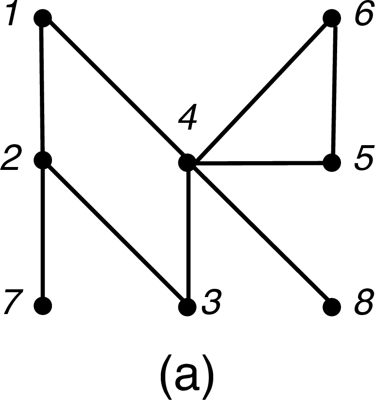
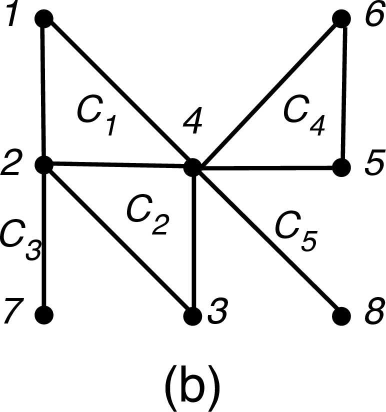
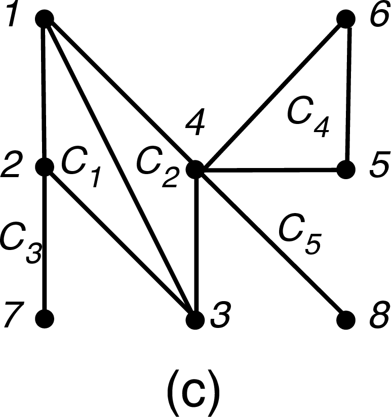
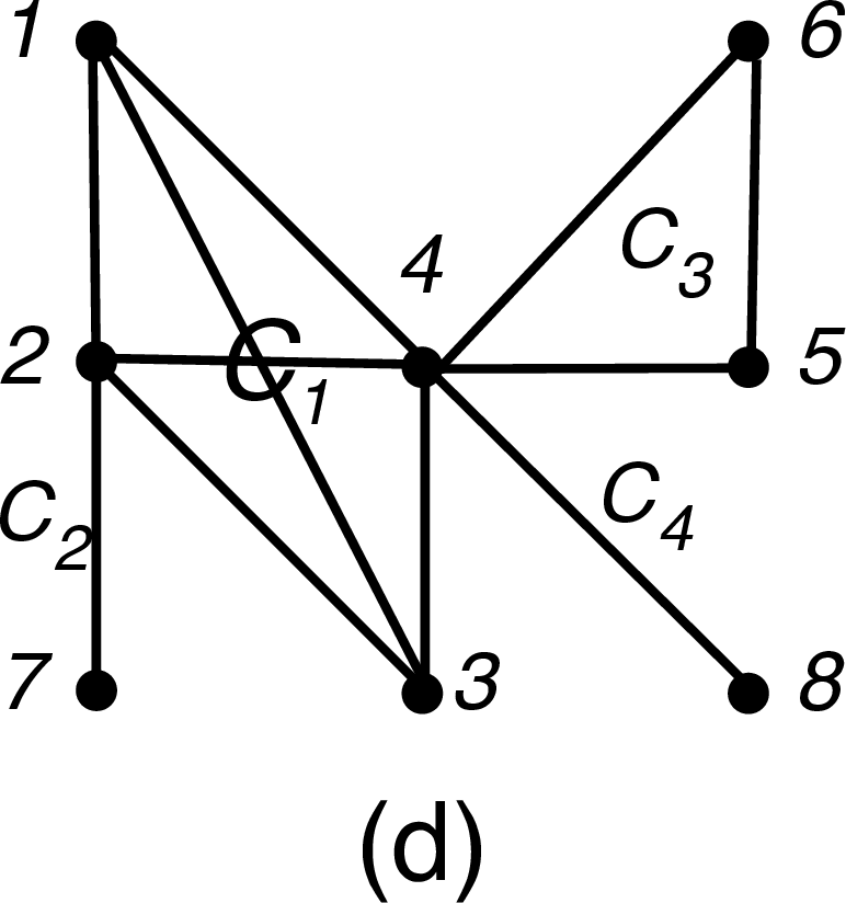
Figure 1: An example of the aggregate sparsity pattern matrix (left),where * denotes nonzero elements. (a) : the associated aggregate sparsitypattern graph \(G(N,\cal E^0)\) with node set \(N = \{1,\ldots,8\}\) and edge set\(\cal E^0 = \{(1,2),(1,4),(2,3),(2,7),(3,4),(4,5),\) \((4,6),(4,8),(5,6)\},\)which is not chordal since the cycle formed by the \(4\) edges \((1,2),(2,3),(3,4),(4,1)\)is a chordless 4-cycle.(b), (c) and (d): chordal extensions of \(G(N,\cal E^0)\). In (b), the maximal cliques are\(C_1=\{1,2,4\},C_2=\{2,3,4\},C_3=\{2,7\},C_4=\{4,5,6\}\), and \(C_5=\{4,8\}\).In (c), the maximal cliques are\(C_1=\{1,2,3\},C_2=\{1,3,4\},C_3=\{2,7\},C_4=\{4,5,6\}\), and \(C_5=\{4,8\}\).In (d), the maximal cliques are\(C_1=\{1,2,3,4\},C_2=\{2,7\},C_3=\{4,5,6\}\), and \(C_4=\{4,8\}\)..
For every nonempty subset \(C\) of \(N\), let \(\mathbb{S}^C\) denote the linear space of \(|C|\times |C|\) symmetric matrices indexed by \(C\times C\), \(\mathbb{S}^C_+\) the cone of positive semidefinite matrices in \(\mathbb{S}^C\), and \(\mathbb{R}^C\) the linear space of \(|C|\)-dimensional column vectors indexed by \(C\). For every \(\boldsymbol{A}\in \mathbb{S}^n\) and every nonempty subset \(C\subseteq N\), we denote by \(\boldsymbol{A}^C \in \mathbb{S}^C\) the principal submatrix of \(\boldsymbol{A}\) indexed by \(C\times C\). Similarly, for every \(\boldsymbol{x}\in \mathbb{R}^n\), we denote by \(\boldsymbol{x}^C \in \mathbb{R}^C\) the subvector indexed by \(C\).
2.3 A clique-wise reformulation of QCQP 1 and its SDP relaxation↩︎
The clique-wise reformulation of QCQP 1 and its SDP relaxation developed below relies on the following well-known results on positive semidefinite matrix completions for chordal graphs [16], [21]. An undirected graph is said to be chordal if every cycle of length at least four has a chord. For an undirected graph \(G(N,\cal E)\), define \(\cal E\cup \{(i,i): i \in N\}\) by \(\overline{\cal E}\). We denote by \(\mathbb{S}^n(\cal E)\) the class of \(n \times n\) partial symmetric matrices \(\boldsymbol{X}\) such that \[\begin{align} & & [\boldsymbol{X}]_{ij}=[\boldsymbol{X}]_{ji}\in \mathbb{R}\quad if(i,j)\in \overline{\cal E}, \; and [\boldsymbol{X}]_{ij}=[\boldsymbol{X}]_{ji} is left unspecified otherwise. \end{align}\] In particular, if \(C\) is a clique of \(G(N,\cal E)\) and \(\boldsymbol{X}\in \mathbb{S}^n(\cal E)\), then the principal submatrix \(\boldsymbol{X}^{C} \in \mathbb{S}^C\) is well-defined since \(C \times C \subseteq \overline{\cal E}\).
Lemma 1. Let \(C_p\) \((p=1,\ldots,\hat{p})\) be the maximal cliques of a chordal graph \(G(N,\cal E)\). Assume that \(\boldsymbol{X}\in \mathbb{S}^n(\cal E)\). Then the following assertions hold.
(i) There exists an \(\overline{\boldsymbol{X}} \in \mathbb{S}^n_+\) such that \([\boldsymbol{X}]_{ij} = [\overline{\boldsymbol{X}}]_{ij}\) for every \((i,j) \in \overline{\cal E}\) if and only if \(\boldsymbol{X}^{C_p} \in \mathbb{S}^{C_p}_+\) \((p=1,\ldots,\hat{p})\). We call such an \(\overline{\boldsymbol{X}} \in \mathbb{S}^n_+\) a positive semidefinite matrix completion of \(\boldsymbol{X}\in \mathbb{S}^n(\cal E)\).
(ii) There exists an \(\overline{\boldsymbol{X}}\in\mathbb{S}^n_+\) such that \([\boldsymbol{X}]_{ij}=[\overline{\boldsymbol{X}}]_{ij}\) for every \((i,j)\in\overline{\cal E}\) and \({\rm rank}(\overline{\boldsymbol{X}})\leq 1\) if and only if \(\boldsymbol{X}^{C_p}\in\mathbb{S}^{C_p}_+\) and \({\rm rank}(\boldsymbol{X}^{C_p})\leq 1\) \((p=1,\ldots,\hat{p})\). We call such an \(\overline{\boldsymbol{X}}\) a rank-at-most-one positive semidefinite matrix completion of \(\boldsymbol{X}\in\mathbb{S}^n(\cal E)\).
In the remainder of the paper, we let \(G(N,\cal E)\) be a chordal extension of the aggregate sparsity pattern graph \(G(N,\cal E^0)\) associated with QCQP 1 . We denote the maximal cliques of \(G(N,\cal E)\) by \(C_p\) \((p=1,\ldots,\hat{p})\). Let \(\overline{\cal E} = \cal E\cup \{(i,i) : i \in N \}\). We note that the aggregate sparsity pattern graph \(G(N,\cal E^0)\) is uniquely determined by the data matrices of QCQP 1 , but that there are multiple chordal extensions in general. Figure 1 illustrates an example of the aggregate sparsity pattern matrix, the aggregate sparsity pattern graph \(G(N,\cal E^0)\), and three different chordal extensions of \(G(N,\cal E^0)\).
Since \(\cal E^0 \subseteq \cal E\subseteq \bigcup_{p=1}^{\hat{p}} ( C_p\times C_p)\), we see that \([\boldsymbol{A}_k]_{ij} = 0\) if \((i,j) \not\in \bigcup_{p=1}^{\hat{p}} (C_p\times C_p)\); hence \[\begin{align} \langle\boldsymbol{A}_k, \, \boldsymbol{X}\rangle = \sum_{(i,j) \in \bigcup_{p=1}^{\hat{p}}( C_p \times C_p)} [\boldsymbol{A}_k]_{ij} [\boldsymbol{X}]_{ij} \; for every\boldsymbol{X}\in \mathbb{S}^n \end{align}\] \((k=0,\ldots,m)\). Let \(k\in \{0,\ldots,m\}\) be fixed. We consider decompositions of the coefficient matrix \(\boldsymbol{A}_k\), a collection of \(\boldsymbol{A}^p_k \in \mathbb{S}^{C_p}\) \((p=1,\ldots,\hat{p})\) such that \[[\boldsymbol{A}_k]_{ij} = \sum_{p \in P(i,j)} [\boldsymbol{A}^p_k]_{ij} \;for every(i,j) \;such thatP(i,j) \ne \emptyset, \label{eq:cliqueDecomposition0}\tag{3}\] where \(P(i,j) = \{ p : (i,j) \in C_p \times C_p\}\). Namely, the \((i,j)\)th element \([\boldsymbol{A}_k]_{ij}\) of \(\boldsymbol{A}_k \in \mathbb{S}^n\) is distributed among \((C_p \times C_p)\)s containing \((i,j)\). Then, \[\langle\boldsymbol{A}_k, \, \boldsymbol{X}\rangle = \sum_{p=1}^{\hat{p}} \langle\boldsymbol{A}_k^p, \, \boldsymbol{X}^{C_p}\rangle \;for every\boldsymbol{X}\in \mathbb{S}^n, \label{eq:cliqueDecomposition}\tag{4}\] or equivalently, \[\sum_{(i,j) \in \bigcup_{p=1}^{\hat{p}}(C_p \times C_p)} [\boldsymbol{A}_k]_{ij}[\boldsymbol{X}]_{ij} = \sum_{p=1}^{\hat{p}} \sum_{(i,j) \in C_p\times C_p} [\boldsymbol{A}_k^p]_{ij}[\boldsymbol{X}]_{ij} \;for every\boldsymbol{X}\in \mathbb{S}^n\] holds. Comparing the terms of symmetric entries \([\boldsymbol{X}]_{ij}\) with \((i,j) \in (C_p \times C_p)\) on both sides of the identity, we see that the left-hand side contains the term \([\boldsymbol{A}_k]_{ij}[\boldsymbol{X}]_{ij}\), while the right-hand side contains \(\sum_{p\in P(i,j)} [\boldsymbol{A}_k^p]_{ij}[\boldsymbol{X}]_{ij}.\) The coefficients of \([\boldsymbol{X}]_{ij}\) are equal by the decomposition defined in 3 . Therefore, the identity holds for every value of \([\boldsymbol{X}]_{ij}\in\mathbb{R}\). This implies 4 . In the case (b) of Figure 1, we see that \(P(2,2) = \{1,2,3\}, P(2,4) = \{1,2\}, P(4,4) = \{1,2,4,5\}.\) Thus, we can take, for example \[\begin{align} & & [\boldsymbol{A}_k^p]_{44} = \frac{[\boldsymbol{A}_k]_{44}}{4} \;for everyp \in P(4,4) = \{1,2,4,5\}or \\ & & [\boldsymbol{A}_k^1]_{44} = [\boldsymbol{A}_k^2]_{44} = [\boldsymbol{A}_k^4]_{44} = 0, \;[\boldsymbol{A}_k^5]_{44} = [\boldsymbol{A}_k]_{44}. \end{align}\]
By substituting identity 4 into QCQP 1 , we obtain an equivalent reformulation of QCQP 1 and its SDP relaxation 2 . \[\begin{align} \zeta_{\rm c} & = & \inf \left\{ \sum_{p=1}^{\hat{p}}\langle\boldsymbol{A}^p_0, \, \boldsymbol{X}^{C_p}\rangle : \begin{array}{l} \boldsymbol{X}\in \mathbb{S}^n(\cal E),\boldsymbol{X}^{C_p} \in \mathbb{S}^{C_p}_+,{\rm rank}(\boldsymbol{X}^{C_p}) \leq 1 \\ (p=1,\ldots,\hat{p}),\\ \displaystyle \sum_{p=1}^{\hat{p}}\langle\boldsymbol{A}^p_k, \, \boldsymbol{X}^{C_p}\rangle \trianglelefteq_k b_k \;(k=1,\ldots,m) \end{array} \right\}. \label{eq:QCQP1} \end{align}\tag{5}\] \[\begin{align} \eta_{\rm c} = \inf \left\{ \sum_{p=1}^{\hat{p}}\langle\boldsymbol{A}^p_0, \, \boldsymbol{X}^{C_p}\rangle : \begin{array}{l} \boldsymbol{X}\in \mathbb{S}^n(\cal E), \boldsymbol{X}^{C_p} \in \mathbb{S}^{C_p}_+ \;(p=1,\ldots,\hat{p}), \\ \displaystyle \sum_{p=1}^{\hat{p}}\langle\boldsymbol{A}^p_k, \, \boldsymbol{X}^{C_p}\rangle \trianglelefteq_k b_k \;(k=1,\ldots,m) \end{array} \right\}. \label{eq:SDP1} \end{align}\tag{6}\] We say that a feasible solution \(\boldsymbol{X}\in\mathbb{S}^n(\cal E)\) of SDP 6 is rank-at-most-one if \[\boldsymbol{X}^{C_p}\in\mathbb{S}^{C_p}_+,\; {\rm rank}(\boldsymbol{X}^{C_p})\leq 1 \;(p=1,\ldots,\hat{p}).\] Thus a rank-at-most-one feasible solution of SDP 6 is precisely a feasible solution of QCQP 5 ; the same terminology is used for optimal solutions. By Lemma 1(ii), an \(\boldsymbol{X}\in\mathbb{S}^n(\cal E)\) is a feasible solution of QCQP 5 if and only if it admits a rank-at-most-one completion \(\overline{\boldsymbol{X}}\in\mathbb{S}^n_+\) that is feasible for the original QCQP 1 . The objective values are the same under this correspondence. Hence QCQP 1 and QCQP 5 are equivalent. Similarly, by Lemma 1(i), the original SDP 2 and SDP 6 are equivalent. Therefore, \(\eta_{\rm c}=\eta\leq \zeta_{\rm c}=\zeta .\) Consequently, the SDP relaxation 2 of QCQP 1 is exact if and only if the SDP relaxation 6 of QCQP 5 is exact, i.e., the SDP relaxation 6 has a rank-at-most-one optimal solution when it has an optimal solution.
Although all constraints in 5 and 6 are expressed in terms of the clique submatrix variables \(\boldsymbol{X}^{C_p} \in \mathbb{S}^{C_p}\) \((p=1,\ldots,\hat{p})\), these variables are not independent in general. Indeed, if two sets \(C_p\) and \(C_q\) overlap, then the corresponding entries of \(\boldsymbol{X}^{C_p}\) and \(\boldsymbol{X}^{C_q}\) must coincide on \((C_p\times C_p)\cap(C_q\times C_q)\). To describe these consistency requirements explicitly, we introduce local matrix variables \(\boldsymbol{Y}^p \in \mathbb{S}^{C_p}\) \((p=1,\ldots,\hat{p})\). Let \[\cal D_p=\bigcup_{q\neq p} \bigl((C_p\cap C_q)\times(C_p\cap C_q)\bigr) \subseteq C_p \times C_p, \;(p=1,\ldots,\hat{p}),\] and define \[\overline{\cal D} = \bigcup_{p=1}^{\hat{p}}\cal D_p = \bigcup_{1\leq p<q\leq \hat{p}} \bigl((C_p\cap C_q)\times(C_p\cap C_q)\bigr).\] Thus, if \(\cal D_p \ne \emptyset\), then \(\cal D_p\) is the set of entries of the local matrix variable \(\boldsymbol{Y}^p\) that are shared with at least one other local matrix variable, and \(\overline{\cal D}\) is the set of all such shared entries. Each \(\cal D_p\) is called a consistency set. The consistency requirement can then be written as \[[\boldsymbol{Y}^p]_{ij}=[\boldsymbol{Y}^q]_{ij} \; whenever(i,j)\in (C_p\cap C_q)\times(C_p\cap C_q) \;andp\neq q.\] Equivalently, we introduce an auxiliary partial symmetric matrix variable \(\boldsymbol{U}\in\mathbb{S}^n(\overline{\cal D})\), called the consistency matrix, and write \[[\boldsymbol{Y}^p]_{ij}=[\boldsymbol{U}]_{ij} \quad ((i,j)\in\cal D_p,\;p=1,\ldots,\hat{p}).\] In this formulation, the clique submatrix variables \(\boldsymbol{X}^{C_p}\) in 5 and 6 are replaced by local matrix variables \(\boldsymbol{Y}^p\). These local matrix variables are linked through the consistency matrix \(\boldsymbol{U}\) on their overlapping entries in the consistency sets \(\cal D_p\) \((p=1,\ldots,\hat{p})\).
We see in case (b) of Figure 1 that \(\cal D_1 = \cal D_2 = \{(2,2),(2,4),(4,4)\}, \cal D_3 = \{(2,2)\}, \cal D_4 = \cal D_5 = \{(4,4)\}\) and in case (d) of Figure 1 that \(\cal D_1 = \{(2,2),(4,4)\}, \cal D_2 = \{(2,2)\}, \cal D_3 = \cal D_4 = \{(4,4)\}\). In the former case (b), the consistency constraints are \[\begin{align} & & [\boldsymbol{Y}^1]_{ij} = [\boldsymbol{Y}^2]_{ij} \;((i,j) \in \{(2,2),(2,4),(4,4)\}), \; [\boldsymbol{Y}^1]_{22} = [\boldsymbol{Y}^3]_{22}, \\ & & [\boldsymbol{Y}^1]_{44} =[\boldsymbol{Y}^2]_{44} =[\boldsymbol{Y}^4]_{44} =[\boldsymbol{Y}^5]_{44}, \end{align}\] while in the latter case (d), they are \[\begin{align} & & [\boldsymbol{Y}^1]_{22} = [\boldsymbol{Y}^2]_{22}, \; [\boldsymbol{Y}^1]_{44} =[\boldsymbol{Y}^3]_{44} =[\boldsymbol{Y}^4]_{44}. \end{align}\] In case (b), the two cliques \(C_1\) and \(C_2\) are coupled not only through the diagonal entries \((2,2)\) and \((4,4)\), but also through the off-diagonal entry \((2,4)\). In contrast, in case (d), all consistency constraints are diagonal.
Consequently, SDP 6 can be rewritten in the local matrix variables \(\boldsymbol{Y}^p\) \((p=1,\ldots,\hat{p})\) and the consistency matrix \(\boldsymbol{U}\) as follows: \[\begin{align} \eta_c = \inf\left\{ \displaystyle \sum_{p=1}^{\hat{p}} \langle\boldsymbol{A}^p_0, \, \boldsymbol{Y}^p\rangle : \begin{array}{l} \boldsymbol{U}\in \mathbb{S}^n(\overline{\cal D}), \; \boldsymbol{Y}^p \in \mathbb{S}^{C_p}_+ \;(p=1,\ldots,\hat{p}), \\ \displaystyle \sum_{p=1}^{\hat{p}} \langle\boldsymbol{A}^p_k, \, \boldsymbol{Y}^p\rangle \trianglelefteq_k b_k \;(k=1,\ldots,m), \\ {[\boldsymbol{Y}^p]_{ij}}=[\boldsymbol{U}]_{ij} \quad ((i,j)\in \cal D_p,\;p=1,\ldots,\hat{p}) \end{array} \right\}. \label{eq:SDP4} \end{align}\tag{7}\] We call 7 the clique-wise formulation of SDP 2 , which was originally proposed in [18]. The problem obtained from SDP 7 by adding a rank-at-most-one condition \[{\rm rank}(\boldsymbol{Y}^p)\leq 1 \quad (p=1,\ldots,\hat{p}) \label{eq:rankOne}\tag{8}\] is called the clique-wise formulation of QCQP 1 . Accordingly, a feasible solution \((\boldsymbol{Y}^1,\ldots,\boldsymbol{Y}^{\hat{p}},\) \(\boldsymbol{U})\) of SDP 7 is called rank-at-most-one if it satisfies 8 . The following two lemmas summarize the relation between the formulations using the partial matrix \(\boldsymbol{X}\) and those using the local matrix variables \(\boldsymbol{Y}^p\) together with the consistency matrix \(\boldsymbol{U}\).
Lemma 2. SDPs 6 and 7 are equivalent. More precisely, the following two assertions hold.
(i) Suppose that \(\boldsymbol{X}\in \mathbb{S}^n(\cal E)\) is a feasible solution of SDP 6 with objective value \(\sum_{p=1}^{\hat{p}}\langle\boldsymbol{A}^p_0, \, \boldsymbol{X}^{C_p}\rangle\). Let \[\boldsymbol{Y}^p=\boldsymbol{X}^{C_p} \;(p=1,\ldots,\hat{p}), \; \boldsymbol{U}\in\mathbb{S}^n(\overline{\cal D}), \; [\boldsymbol{U}]_{ij}=[\boldsymbol{X}]_{ij} \;((i,j)\in\overline{\cal D}).\] Then \((\boldsymbol{Y}^1,\ldots,\boldsymbol{Y}^{\hat{p}},\boldsymbol{U})\) is a feasible solution of SDP 7 with the same objective value.
(ii) Suppose that \((\boldsymbol{Y}^1,\ldots,\boldsymbol{Y}^{\hat{p}},\boldsymbol{U})\) is a feasible solution of SDP 7 with objective value \(\sum_{p=1}^{\hat{p}}\langle\boldsymbol{A}^p_0, \, \boldsymbol{Y}^p\rangle\). Then there exists a feasible solution \(\boldsymbol{X}\in\mathbb{S}^n(\cal E)\) of SDP 6 satisfying \(\boldsymbol{X}^{C_p}=\boldsymbol{Y}^p \;(p=1,\ldots,\hat{p})\) with the same objective value.
Lemma 3. QCQP 5 is equivalent to SDP 7 with the additional rank-at-most-one condition 8 . More precisely, the following two assertions hold.
(i) Suppose that \(\boldsymbol{X}\in \mathbb{S}^n(\cal E)\) is a feasible solution of QCQP 5 with objective value \(\sum_{p=1}^{\hat{p}}\langle\boldsymbol{A}^p_0, \, \boldsymbol{X}^{C_p}\rangle\). Let \[\boldsymbol{Y}^p=\boldsymbol{X}^{C_p} \;(p=1,\ldots,\hat{p}), \; \boldsymbol{U}\in\mathbb{S}^n(\overline{\cal D}), \; [\boldsymbol{U}]_{ij}=[\boldsymbol{X}]_{ij} \;((i,j)\in\overline{\cal D}).\] Then \((\boldsymbol{Y}^1,\ldots,\boldsymbol{Y}^{\hat{p}},\boldsymbol{U})\) is a rank-at-most-one feasible solution of the SDP 7 with the same objective value.
(ii) Suppose that \((\boldsymbol{Y}^1,\ldots,\boldsymbol{Y}^{\hat{p}},\boldsymbol{U})\) is a rank-at-most-one feasible solution of SDP 7 with objective value \(\sum_{p=1}^{\hat{p}}\langle\boldsymbol{A}^p_0, \, \boldsymbol{Y}^p\rangle\). Then there exists a feasible solution \(\boldsymbol{X}\in\mathbb{S}^n(\cal E)\) of QCQP 5 satisfying \(\boldsymbol{X}^{C_p}=\boldsymbol{Y}^p \;(p=1,\ldots,\hat{p})\) with the same objective value.
By Lemmas 1, 2 and 3, we have shown that SDP 2 and QCQP 1 are equivalent to their clique-wise formulations, SDP 7 and SDP 7 with the additional rank-at-most-one condition 8 , respectively. Consequently, SDP 2 has a rank-at-most-one optimal solution \(\boldsymbol{X}\), which is an optimal solution of QCQP 1 , if and only if SDP 7 has a rank-at-most-one optimal solution \((\boldsymbol{Y}^1,\ldots,\boldsymbol{Y}^{\hat{p}},\boldsymbol{U})\) such that \(\boldsymbol{X}^{C_p} = \boldsymbol{Y}^p\) \((p=1,\ldots,\hat{p})\). This equivalence allows the exactness analysis of the original SDP relaxation 2 to be carried out through the clique-wise formulation 7 .
It should be noted that the choice of decompositions of the coefficient matrices \(\boldsymbol{A}_k \in \mathbb{S}^n\) into collections \(\boldsymbol{A}^p_k \in \mathbb{S}^{C_p}\) \((p=1,\ldots,\hat{p})\) satisfying 3 does not affect the equivalence of SDP 2 with SDP 7 . The choice can, however, affect the local sub-SDP 9 in the single matrix variable \(\boldsymbol{Y}^p\), introduced in the next section, where the matrices \(\boldsymbol{A}^p_k\) \((k=0,\ldots,m)\) appear explicitly in the objective and constraint functions \((p=1,\ldots,\hat{p})\).
3 Local-to-global exactness via clique subproblems↩︎
Throughout the remainder of the paper, SDP 7 is referred to as the global SDP. For each clique \(C_p\) \((p=1,\ldots,\hat{p})\), we introduce a local sub-SDP, denoted by SDP 9 , which describes the corresponding local component of the global SDP when the local right-hand-side and consistency matrix are fixed. The purpose of this section is to relate the exactness of the global SDP 7 to the exactness of the associated local sub-SDPs.
3.1 Clique-wise subproblems↩︎
For \(p=1,\ldots,\hat{p}\), we define a local sub-SDP in the local matrix variable \(\boldsymbol{Y}^p\) associated with the clique \(C_p\) by fixing a vector \(\boldsymbol{\delta}^p = (\delta^p_1,\ldots,\delta^p_m) \in \mathbb{R}^m\) and a consistency matrix \(\boldsymbol{U}\in \mathbb{S}^n(\overline{\cal D})\) as parameters. The parameter \(\delta_k^p\) represents the distribution of each global constraint right-hand side constant \(b_k\) into local constraint right-hand side constants of the sub-SDPs \((k=1,\ldots,m)\), while the other parameter, consistency matrix \(\boldsymbol{U}\) specifies the values of the entries of the local matrix variable \(\boldsymbol{Y}^p\) shared by different cliques, i.e., it fixes the entries of \(\boldsymbol{Y}^p\) on \(\cal D_p\) so as to enforce consistency among overlapping cliques. We now define the corresponding local sub-SDP as follows: \[\eta^p_c(\boldsymbol{\delta}^p,\boldsymbol{U}) = \inf \left\{ \langle \boldsymbol{A}^p_0, \boldsymbol{Y}^p \rangle : \begin{array}{l} \boldsymbol{Y}^p \in \mathbb{S}^{C_p}_+, \\ \langle \boldsymbol{A}^p_k, \boldsymbol{Y}^p \rangle \trianglelefteq_k \delta^p_k \;(k=1,\ldots,m),\\[3pt] {[\boldsymbol{Y}^p]_{ij}} = [\boldsymbol{U}]_{ij} \;((i,j)\in \cal D_p) \end{array} \right\}. \label{eq:subSDP}\tag{9}\] The sub-SDP 9 is the local problem associated with \(C_p\), obtained from the global SDP 7 by fixing parameters \((\boldsymbol{\delta}^p,\boldsymbol{U})\). It will be used to characterize the exactness of SDP 7 . If the rank-at-most-one condition rank(\(\boldsymbol{Y}^p) \leq 1\) is added to sub-SDP 9 , then we obtain a local sub-QCQP.
In the example illustrated in Figure 1(d), there are four local sub-SDPs associated with \(C_1,C_2,C_3,C_4\). These sub-SDPs are coupled only through the consistency matrix \(\boldsymbol{U}\in \mathbb{S}^n(\overline{\cal D})\) via the consistency constraints \([\boldsymbol{Y}^p]_{ij}=[\boldsymbol{U}]_{ij}\) for \((i,j)\in\cal D_p\) \((p=1,\ldots,4)\), where \(\cal D_1 = \{(2,2),(4,4)\}, \cal D_2 = \{(2,2)\}, \cal D_3 = \{(4,4)\}, \cal D_4 = \{(4,4)\}.\)
The connection between the local sub-SDPs 9 \((p=1,\ldots,\hat{p})\) and the global SDP 7 can be expressed through a bilevel optimization problem. In this representation, the upper level determines the local right-hand-side vectors \(\boldsymbol{\delta}^p\) \((p=1,\ldots,\hat{p})\), and the common consistency matrix \(\boldsymbol{U}\), while the lower level consists of the local sub-SDPs 9 . The upper-level objective is the sum of the lower-level optimal values \(\eta^p_c(\boldsymbol{\delta}^p,\boldsymbol{U})\) \((p=1,\ldots,\hat{p})\). Define the upper-level problem associated with the global SDP by \[\begin{align} \widetilde{\eta}_c &=& \inf\left\{ \sum_{p=1}^{\hat{p}} \eta^p_c(\boldsymbol{\delta}^p,\boldsymbol{U}) : \begin{array}{l} \eta^p_c(\boldsymbol{\delta}^p,\boldsymbol{U}) < +\infty \quad (p=1,\ldots,\hat{p}), \\ \displaystyle \sum_{p=1}^{\hat{p}} \delta^p_k \trianglelefteq_k b_k \quad (k=1,\ldots,m), \\ \boldsymbol{U}\in \mathbb{S}^n(\overline{\cal D}) \end{array} \right\}. \label{eq:bilevelSDP} \end{align}\tag{10}\] The conditions \(\eta^p_c(\boldsymbol{\delta}^p,\boldsymbol{U})<+\infty\) \((p=1,\ldots,\hat{p})\) exclude infeasible local subproblems. However, they do not exclude local subproblems with optimal value \(-\infty\) at this stage.
Lemma 4. The problem 10 has the same optimal value as SDP 7 ; that is, \(\widetilde{\eta}_c=\eta_c .\)
3.2 Relation between the global SDP and local sub-SDPs↩︎
The following theorem is the main result of the paper. It provides a local-to-global exactness framework for the clique-wise formulation. Specifically, an optimal solution \((\widetilde{\boldsymbol{Y}}^1,\ldots,\widetilde{\boldsymbol{Y}}^{\hat{p}},\widetilde{\boldsymbol{U}})\) of the global clique-wise SDP 7 induces the local right-hand-side vectors \(\tilde{\boldsymbol{\delta}}^p\) \((p=1,\ldots,\hat{p})\) and the consistency matrix \(\widetilde{\boldsymbol{U}}\). The relevant local sub-SDPs 9 are precisely those defined by these induced parameters. If these induced local sub-SDPs admit rank-at-most-one optimal solutions, then exactness of the original SDP relaxation follows.
Theorem 5. Let \((\widetilde{\boldsymbol{Y}}^1,\ldots,\widetilde{\boldsymbol{Y}}^{\hat{p}},\widetilde{ \boldsymbol{U}})\) be an optimal solution of SDP 7 . Define \[\begin{align} & & \tilde{\boldsymbol{\delta}}^p \in \mathbb{R}^m, \; \tilde{\delta}^p_k = \langle\boldsymbol{A}^p_k, \, \widetilde{\boldsymbol{Y}}^p\rangle \;(k=1,\ldots,m, \;p=1,\ldots,\hat{p}). \label{eq:bdelta} \end{align}\qquad{(1)}\] Then the following assertions hold:
(i) Each \(\widetilde{\boldsymbol{Y}}^p\) is an optimal solution of sub-SDP 9 with the parameters \((\boldsymbol{\delta}^p,\boldsymbol{U}) = (\tilde{\boldsymbol{\delta}}^p,\widetilde{\boldsymbol{U}})\); hence \(\langle\boldsymbol{A}^p_0, \, \widetilde{\boldsymbol{Y}}^p\rangle = \eta^p_c(\tilde{\boldsymbol{\delta}}^p,\widetilde{\boldsymbol{U}})\) \((p=1,\ldots,\hat{p})\) and \(\sum_{p=1}^{\hat{p}} \eta^p_c(\tilde{\boldsymbol{\delta}}^p,\widetilde{\boldsymbol{U}}) = \sum_{p=1}^{\hat{p}} \langle\boldsymbol{A}^p_0, \, \widetilde{\boldsymbol{Y}}^p\rangle = \eta_c\).
(ii) For \(p =1,\ldots,\hat{p}\), let \(\widehat{\boldsymbol{Y}}^p \in \mathbb{S}^{C_p}_+\) be an optimal solution of sub-SDP 9 with the parameters \((\boldsymbol{\delta}^p,\boldsymbol{U}) = (\tilde{\boldsymbol{\delta}}^p,\widetilde{\boldsymbol{U}})\); hence \(\langle\boldsymbol{A}^p_0, \, \widehat{\boldsymbol{Y}}^p\rangle = \eta^p_c(\tilde{\boldsymbol{\delta}}^p,\widetilde{\boldsymbol{U}})\). Then \((\widehat{\boldsymbol{Y}}^1,\ldots,\widehat{\boldsymbol{Y}}^{\hat{p}},\widetilde{ \boldsymbol{U}})\) is an optimal solution of SDP 7 , and therefore \(\eta_c = \sum_{p=1}^{\hat{p}}\langle\boldsymbol{A}^p_0, \, \widehat{\boldsymbol{Y}}^p\rangle\).
(iii) Assume that, for \(p =1,\ldots,\hat{p}\), sub-SDP 9 with the parameters \((\boldsymbol{\delta}^p,\boldsymbol{U}) = (\tilde{\boldsymbol{\delta}}^p,\widetilde{\boldsymbol{U}})\) is exact. Then SDP 7 is exact.
3.3 Diagonal consistency assumption↩︎
Theorem 5(iii) requires exactness of the local sub-SDPs 9 with the parameters \((\boldsymbol{\delta}^p,\boldsymbol{U})=(\tilde{\boldsymbol{\delta}}^p,\widetilde{\boldsymbol{U}})\) induced by an optimal solution of the global SDP 7 \((p=1,\ldots,\hat{p})\). These parameters are not known a priori. Therefore, in order to use the theorem together with local exactness results, it is necessary to identify classes of local sub-SDPs whose exactness can be guaranteed for all admissible parameter values, or under conditions that can be checked without solving the global SDP.
A critical obstruction for identifying such classes of sub-SDPs is caused by the unknown consistency matrix \(\widetilde{\boldsymbol{U}}\). To see this, focus only on the consistency constraints in the sub-SDP 9 with the parameter \((\boldsymbol{\delta}^p,\boldsymbol{U})=(\tilde{\boldsymbol{\delta}}^p,\widetilde{\boldsymbol{U}})\), \[[\boldsymbol{Y}^p]_{ij}=[\widetilde{\boldsymbol{U}}]_{ij} \quad ((i,j)\in\cal D_p).\] For these constraints to be satisfied by an unknown rank-at-most-one optimal solution \(\widetilde{\boldsymbol{Y}}^p\) of the sub-SDP 9 , the entries of \(\widetilde{\boldsymbol{U}}\) must satisfy the necessary condition \[[\boldsymbol{u}]_i[\boldsymbol{u}]_j = [\widetilde{\boldsymbol{U}}]_{ij} \quad ((i,j)\in\cal D_p) \quad for some\boldsymbol{u}\in \mathbb{R}^{C_p}. \label{eq:compRelation}\tag{11}\] Thus, when the consistency set \(\cal D_p\) contains off-diagonal entries, the consistency matrix \(\widetilde{\boldsymbol{U}}\) must satisfy the nontrivial product relations 11 . If 11 is not satisfied, the sub-SDP 9 cannot have a rank-at-most-one feasible solution. Also, 11 cannot be verified in advance since the consistency matrix \(\widetilde{\boldsymbol{U}}\) is unknown.
To avoid this obstruction, we impose the following diagonal consistency assumption: \[\cal D_p \subseteq \{(i,i): i\in N\} \quad (p=1,\ldots,\hat{p}). \label{eq:blockClique}\tag{12}\] Equivalently, any two distinct maximal cliques intersect in at most one node, \[|C_p\cap C_q|\leq 1 \quad (p\ne q).\] A chordal graph satisfying this assumption is called a block-clique graph [22], [23]. Under the diagonal consistency assumption, 11 reduces to the simpler necessary condition \[([\boldsymbol{u}]_i)^2 = [\widetilde{\boldsymbol{U}}]_{ii} \quad ((i,i)\in\cal D_p) \quad for some\boldsymbol{u}\in \mathbb{R}^{C_p}.\] Since \([\widetilde{\boldsymbol{U}}]_{ii}=[\widetilde{\boldsymbol{Y}}^p]_{ii}\geq0\) for every \((i,i)\in\cal D_p\), this condition is always satisfied, and the obstruction 11 on the unknown consistency matrix \(\widetilde{\boldsymbol{U}}\) caused by off-diagonal entries in \(\cal D_p\) has been removed.
It is important to note that the block-clique assumption does not imply exactness of the sub-SDP 9 . Its role is to remove the off-diagonal product obstruction on \(\widetilde{\boldsymbol{U}}\) caused by 11 when applying Theorem 5(iii). Thus the block-clique assumption makes it possible to formulate local exactness results in Section 4 without having to verify unknown off-diagonal product relations 11 on the consistency matrix \(\widetilde{\boldsymbol{U}}\).
The diagonal consistency assumption 12 leads to the following three representative cases of the consistency set \(\cal D_p\):
(0) \(\cal D_p=\emptyset\).
(I) \(\cal D_p=\{(i,i)\}\) for some \(i\in C_p\).
(II) \(\{(i,i):i\in C_p\} \supseteq \cal D_p\) with multiple diagonal indices.
In case (0), the local matrix variable \(\boldsymbol{Y}^p\) is not subject to any consistency constraints. The corresponding subproblem is therefore independent of the other local sub-SDPs at the level of matrix variables, although coupling may still occur through the right-hand-side parameter vector \(\boldsymbol{\delta}^p\).
In case (I), the consistency constraints fix one diagonal entry of the local matrix variable \(\boldsymbol{Y}^p\). This occurs when the clique \(C_p\) shares a single node with another clique, as illustrated in the cases of \(\cal D_2\), \(\cal D_3\), and \(\cal D_4\) in Figure 1(d), where \([\boldsymbol{Y}^2]_{22}=[\boldsymbol{U}]_{22}\), \([\boldsymbol{Y}^3]_{44}=[\boldsymbol{U}]_{44}\), and \([\boldsymbol{Y}^4]_{44}=[\boldsymbol{U}]_{44}\) are consistency constraints, respectively.
In case (II), multiple diagonal entries of the local matrix variable \(\boldsymbol{Y}^p\) are fixed through the consistency matrix \(\boldsymbol{U}\). This may occur when \(C_p\) intersects several other cliques, each in a single node. This is illustrated by the case of \(C_1\) in Figure 1(d), where the consistency constraints are \([\boldsymbol{Y}^1]_{22}=[\boldsymbol{U}]_{22}\) and \([\boldsymbol{Y}^1]_{44}=[\boldsymbol{U}]_{44}\).
In the next section, we identify three classes of local sub-QCQPs whose SDP relaxations admit rank-at-most-one optimal solutions under this diagonal consistency assumption 12 . These classes provide local building blocks for the local-to-global exactness framework.
4 Sub-QCQPs with exact SDP relaxations↩︎
In this section, we present three classes of local sub-QCQPs whose corresponding local sub-SDPs are exact. These are: convex sub-QCQPs, sub-QCQPs characterized by sign-pattern conditions, and separable sub-QCQPs with a limited number of constraints. Sections 4.1, 4.2, and 4.3 discuss these three classes, respectively. For example, in Figure 1(d), different classes can be assigned to different clique-wise subproblems. Further examples will be presented in Section 5.
The first two classes have a parameter-independent character: their local SDP relaxations are exact for every right-hand-side vector and consistency matrix. By contrast, the exactness of the third class may depend on the right-hand-side vector induced from an optimal solution of the global SDP. This distinction is important when the local exactness results are combined through Theorem 5(iii).
For notational simplicity, we fix a clique \(C_p\) throughout this section and suppress the superscript \(p\). Thus we write \(C_p=C=\{1,\ldots,\ell\}\), \(\boldsymbol{A}^p_k=\boldsymbol{A}_k\), \(\boldsymbol{\delta}^p=\boldsymbol{\delta}\), and \(\cal D_p=\cal D\). Under the diagonal consistency assumption 12 , we have \(\cal D\subseteq\{(i,i):1\le i\le \ell\}\). Then the local sub-SDP is written as \[\eta(\boldsymbol{\delta},\boldsymbol{U}) = \inf \left\{ \langle \boldsymbol{A}_0,\boldsymbol{Y}\rangle : \begin{array}{l} \boldsymbol{Y}\in \mathbb{S}^{\ell}_+, \\ \langle \boldsymbol{A}_k, \boldsymbol{Y}\rangle \trianglelefteq_k \delta_k \;(k=1,\ldots,m),\\[3pt] {[\boldsymbol{Y}]_{ii}} = U_{ii} \;((i,i)\in \cal D) \end{array} \right\}. \label{eq:subSDP1}\tag{13}\] We call the problem obtained by adding \({\rm rank}(\boldsymbol{Y})\leq1\) to SDP 13 the local sub-QCQP.
4.1 Sub-QCQPs characterized by convexity↩︎
Theorem 6. Assume that ‘\(\trianglelefteq_k\)’ \(=\) ‘\(\le\)’ \((1 \leq k \leq m)\). Suppose that one of the following conditions holds:
(0) \(\cal D= \emptyset\) and \(\boldsymbol{A}_k\) \((k=0,\ldots,m)\) are positive semidefinite.
(I) \(\cal D= \{(i,i)\}\) for some \(i \in C\) and \(\boldsymbol{A}_k^{C\backslash\{i\}}\) \((k=0,\ldots,m)\) are positive semidefinite.
Then, sub-SDP 13 is exact, i.e., sub-SDP 13 has a rank-at-most-one optimal solution whenever it has an optimal solution, for every \(\boldsymbol{\delta}\in\mathbb{R}^m\) and \(\boldsymbol{U}\in \mathbb{S}^{\ell}(\cal D)\).
We note that, except for the assumptions in (0) and (I), no additional assumption is required on the right-hand-side vector \(\boldsymbol{\delta}\) or the consistency matrix \(\boldsymbol{U}\).
4.2 Sub-QCQPs characterized by sign-pattern conditions↩︎
We next consider a class of generally nonconvex sub-QCQPs whose SDP relaxations are exact under suitable sign-pattern conditions on the data matrices \(\boldsymbol{A}_k\) \((0\leq k \leq m)\). Throughout this section, we assume that \(\trianglelefteq_k\) \(=\) ‘\(\le\)’ \((1 \leq k \leq m)\). As in the convex case, the exactness result for this class holds for every right-hand-side vector \(\boldsymbol{\delta}\) and consistency matrix \(\boldsymbol{U}\). Let \(G(L,\cal F)\) denote the aggregate sparsity pattern graph with the node set \(L = \{1,\ldots,\ell\}\) and \[\begin{align} \cal F& = & \left\{ (i,j) \in L \times L : i \not= j, \;[\boldsymbol{A}_k]_{ij} \ne 0 \;for somek \in \{0,1,\ldots,m\} \right\}. \end{align}\] We assume that \(\cal D\subseteq \{(i,i) : i \in C\}\) and \(0 \leq |\cal D| \leq \ell\) (case (II)). Note that the equality constraints \([\boldsymbol{Y}]_{ii} = U_{ii}\) \(((i,i) \in \cal D)\) in sub-SDP 13 and the corresponding sub-QCQP can be replaced by the inequality constraints \([\boldsymbol{Y}]_{ii} \leq U_{ii}, \;-[\boldsymbol{Y}]_{ii} \leq -U_{ii} \;((i,i) \in \cal D).\) These inequality constraints, however, do not affect the aggregate sparsity pattern graph \(G(L,\cal F)\) of their data matrices.
For every \((i,j) \in \cal F\), define \[\begin{align} \sigma_{ij} = \begin{cases} +1 & \text{if } [\boldsymbol{A}_k]_{ij} \ge 0 \text{ for all } k \in \{0,1,\ldots,m\},\\ -1 & \text{if } [\boldsymbol{A}_k]_{ij} \le 0 \text{ for all } k \in \{0,1,\ldots,m\},\\ 0 & \text{otherwise}. \end{cases} \end{align}\] Let \(\{F_1,\ldots,F_r\}\) denote a cycle basis for \(G(L,\cal F)\). The following theorem and its corollary follow directly from [7], respectively.
Theorem 7. ([7]) Assume that
(i) \(\sigma_{ij} \in \{-1,1\} \;for every (i,j) \in \cal F\),
(ii) \(\prod_{(i,j)\in F_s} \sigma_{ij} = (-1)^{|F_s|} for every s=1,\ldots,r\).
Then sub-SDP 13 is exact for every \(\boldsymbol{\delta}\in\mathbb{R}^m\) and \(\boldsymbol{U}\in \mathbb{S}^{\ell}(\cal D)\).
Corollary 8. ([7]) Assume that one of the following conditions holds:
(i) The graph \(G(L,\cal F)\) is arbitrary and \(\sigma_{ij} = -1\) for every \((i,j) \in \cal F\) (or equivalently all off-diagonal elements of \(\boldsymbol{A}_k\) are nonpositive, i.e., \(\boldsymbol{A}_k\) is a symmetric \(Z\)-matrix \((0 \leq k \leq m)\)).
(ii) The graph \(G(L,\cal F)\) is a forest and \(\sigma_{ij} \in \{ -1,1\}\) for every \((i,j) \in \cal F\).
(iii) The graph \(G(L,\cal F)\) is bipartite and \(\sigma_{ij} = 1\) for every \((i,j) \in \cal F\).
Then sub-SDP 13 is exact for every \(\boldsymbol{\delta}\in\mathbb{R}^m\) and \(\boldsymbol{U}\in \mathbb{S}^{\ell}(\cal D)\). The condition (i) originally was proposed in [6] for SDP exactness.
The theorem and corollary above establish exactness for every local sub-SDP in this sign-pattern class. Thus, under the diagonal consistency assumption 12 , this class is parameter-independent: once the sign-pattern conditions are satisfied, no further assumption is required on the right-hand-side vector \(\boldsymbol{\delta}\) or the consistency matrix \(\boldsymbol{U}\).
4.3 Separable sub-QCQPs characterized by a limited number of constraints↩︎
We now consider a class of separable sub-QCQPs whose objective and constraint functions share a separable structure. In contrast to the classes considered in Sections 4.1 and 4.2, exactness of the corresponding SDP relaxations is not guaranteed by structural properties. It depends on the number of constraints and the right-hand-side vector \(\boldsymbol{\delta}\) induced by the global problem. Exactness of the SDP relaxation for this class follows from a rank argument ([9]) that depends on the number of constraints relative to the number of separable blocks. This dependence explains why the class must be treated separately: when a separable subproblem appears as a clique-wise component of the global SDP, the relevant right-hand-side vector \(\boldsymbol{\delta}\) is not chosen independently, but is induced by an optimal solution of the global problem.
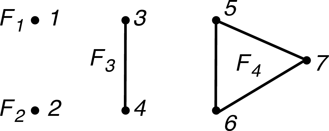
To describe the sub-SDP corresponding to a separable sub-QCQP, we impose the following condition on sub-SDP 13 :
(A) All the data matrices \(\boldsymbol{A}_k\) \((k=0,\ldots,m)\) share a common block-diagonal structure. We denote the \(q\)th diagonal block of each \(\boldsymbol{A}_k\) by \(\boldsymbol{B}^q_k \in \mathbb{S}^{F_q}\) \((q=1,\ldots,\hat{q})\), where \(\{ F_q: q=1,\ldots,\hat{q}\}\) is a partition of \(C = \{1,\ldots,\ell\}\) such that \(i < j\) if \(i \in F_q\), \(j \in F_r\) and \(q < r\). We simply write \(\boldsymbol{A}_k = {\rm diag}(\boldsymbol{B}^1_k,\ldots,\boldsymbol{B}^{\hat{q}}_k)\).
In this case, sub-SDP 13 possesses a block-diagonal sparsity structure. Its aggregate sparsity pattern graph itself is chordal and consists of \(\hat{q}\) disjoint cliques \(F_q\) \((q=1,\ldots,\hat{q})\). See Figure 2, where \(\ell = 7\), \(\hat{q} = 4\), \(F_1 = \{1\}, F_2 = \{2\}, F_3 = \{3,4\}\) and \(F_4 = \{5,6,7\}\).
Let \(\cal D_q = \cal D\cap(F_q\times F_q),\;(q=1,\ldots,\hat{q})\), where the consistency set \(\cal D\subseteq \{(i,i) : 1 \leq i \leq \ell\}\) is given for sub-SDP 13 . Then we can convert sub-SDP 13 further into a clique-wise SDP as follows. \[\begin{align} \eta(\boldsymbol{\delta},\boldsymbol{U}) = \inf\left\{ \displaystyle \sum_{q=1}^{\hat{q}} \langle\boldsymbol{B}^q_0, \, \boldsymbol{W}^q\rangle : \begin{array}{l} \boldsymbol{W}^q \in \mathbb{S}^{F_q}_+ \;(q=1,\ldots,\hat{q}), \\ \displaystyle \sum_{q=1}^{\hat{q}} \langle\boldsymbol{B}^q_k, \, \boldsymbol{W}^q\rangle \trianglelefteq_k \delta_k \;(k=1,\ldots,m), \\ {[\boldsymbol{W}^q]_{ii}}=U_{ii} \;((i,i)\in \cal D_q,\;q=1,\ldots,\hat{q}) \end{array} \right\}. \label{eq:subSDP4} \end{align}\tag{14}\]
Under Condition (A), Lemma 1 shows that sub-SDP 13 is equivalent to SDP 14 . SDP 14 is interpreted as a separable problem because the matrix variables \(\boldsymbol{W}^q \in \mathbb{S}^{F_q}\) \((q=1,\ldots,\hat{q})\) do not overlap, i.e., \(F_q\cap F_r=\emptyset\) \((q\ne r)\).
Theorem 9. Assume that Condition (A) is satisfied, so that sub-SDP 13 is equivalent to SDP 14 . Let \(\boldsymbol{\delta}\in \mathbb{R}^m\) and \(\boldsymbol{U}\in \mathbb{S}^{\ell}(\cal D)\). Define \[\mu = the number of elements in\left\{(i,i)\in \cal D: U_{ii} > 0\right\}.\] Assume that
(B) For every optimal solution \((\boldsymbol{W}^1,\ldots,\boldsymbol{W}^{\hat{q}})\) of SDP 14 , at least \(m+\mu-1\) members of the following collection are nonzero: \[\{\boldsymbol{W}^q : q=1,\ldots,\hat{q}\} \;\cup\; \left\{ \delta_k - \sum_{q=1}^{\hat{q}}\langle\boldsymbol{B}^q_k, \, \boldsymbol{W}^q\rangle : k=1,\ldots,m \right\}.\]
Then SDP 13 is exact.
It should be noted that Condition (B) involves \(\boldsymbol{U}\in \mathbb{S}^{\ell}(\cal D)\), which determines \(\mu\), and \(\boldsymbol{\delta}= (\delta_1,\ldots,\delta_m) \in \mathbb{R}^m\). Thus, exactness of sub-SDP 13 depends not only on the number \(m\) of constraints, but also on the right-hand-side vector \(\boldsymbol{\delta}\in \mathbb{R}^m\) and the consistency matrix \(\boldsymbol{U}\in \mathbb{S}^{\ell}(\cal D)\). In Theorem 5, these are not free parameters: they are induced by an optimal solution \((\widetilde{\boldsymbol{Y}}^1,\ldots,\widetilde{\boldsymbol{Y}}^{\hat{p}},\widetilde{\boldsymbol{U}})\) of the global SDP 7 , with \(\boldsymbol{\delta}\) corresponding to one of the \(\tilde{\boldsymbol{\delta}}^p\) \((p=1,\ldots,\hat{p})\), and \(\boldsymbol{U}\) corresponding to \(\widetilde{\boldsymbol{U}}\). Consequently, when SDP 14 appears as a local sub-SDP within the global SDP, its exactness may depend on the behavior of the other local sub-SDPs. This dependence distinguishes the present separable class from the parameter-independent classes based on convexity or sign-pattern conditions.
Remark 10. Theorem 9 can be compared with the result in [4], where the following assumptions were imposed: \[\begin{align} & & m \leq {\hat{q}}+1, \;\cal D_q = \emptyset \;(q=1,\ldots,\hat{q}) \;(hence \mu = 0), \\ & & \boldsymbol{W}^q \not= \boldsymbol{O}\;(1 \leq q \leq \hat{q}) \;for every optimal solution(\boldsymbol{W}^1,\ldots,\boldsymbol{W}^{\hat{q}}). \end{align}\] Under these assumptions, [eq:rankCond] implies \[\begin{align} m-1 \leq {\hat{q}} \leq \sum_{q=1}^{\hat{q}} \frac{rank(\widetilde{\boldsymbol{W}}^q)(rank(\widetilde{\boldsymbol{W}}^q)+1)}{2} \leq m, \end{align}\] and hence either \(\hat{q} = m-1\) or \(\hat{q} = m\), that is, either \(m=\hat{q}+1\) or \(m=\hat{q}\). In contrast, Condition (B) of Theorem 9 considerably relaxes this restriction.
Even in case \(\cal D_q=\emptyset\) \((q =1,\ldots,\hat{q})\), whether Condition (B) holds depends on the right-hand-side vector \(\boldsymbol{\delta}\) and the relations ‘\(\trianglelefteq_k\)’ \((1 \le k \le m)\). When \(m + |\cal D| \leq 2\), the conclusion of Theorem 9 holds without any additional assumptions on \(\boldsymbol{\delta}\), the relations ‘\(\trianglelefteq_k\)’, and \(\boldsymbol{B}^q_k\) \((q=1,\ldots, {\hat{q}}, \;k=0,\ldots,m)\), and the number \(\hat{q}\) of the separable blocks as shown below. (This result is known; see [10], [24], [25].)
4.4 Preserving the exactness of sub-SDP 13 by adding dependent inequality constraints↩︎
The following theorem establishes a preservation result for a family of sub-SDPs with varying right-hand-side vectors. Assume that sub-SDP 13 has a rank-at-most-one optimal solution for every right-hand-side vector whenever its optimal value is finite and attained. Then inequality constraints whose coefficient matrices lie in the conic hull of the coefficient matrices of the existing constraints may be added without destroying exactness. Thus, the resulting modified sub-SDP is exact.
Theorem 12. Assume that \(\trianglelefteq_k=\) ‘\(\le\)’ \((k=1,\ldots,m)\) and \(\boldsymbol{U}\in\mathbb{S}^\ell(\cal D)\). Suppose that, for every \(\boldsymbol{\delta}'\in\mathbb{R}^m\), if \(-\infty < \eta(\boldsymbol{\delta}',\boldsymbol{U}) < \infty\), then SDP 13 with \(\boldsymbol{\delta}=\boldsymbol{\delta}'\) has a rank-at-most-one optimal solution. Let \(\boldsymbol{\delta}\in\mathbb{R}^m\) and \(\delta_j\in\mathbb{R}\) \((j=m+1,\ldots,m')\) be fixed, where \(m < m'\). Assume that \[\begin{align} & & \boldsymbol{A}_j\in \rm cone\{\boldsymbol{A}_k:k=1,\ldots,m\} \equiv \left\{ \sum_{k=1}^m \alpha_k\boldsymbol{A}_k : \alpha_k \geq 0 \;(k=1,\ldots,m) \right\} \\ & &(j=m+1,\ldots,m'). \end{align}\] Then the modified SDP obtained from SDP 13 by adding the constraints \[\langle\boldsymbol{A}_j, \, \boldsymbol{Y}\rangle\leq \delta_j \;(j=m+1,\ldots,m')\] is exact.
The proof above shows that, although the additional constraints may shrink the feasible region, they become redundant after replacing the right-hand-side vector by the values attained at an optimal solution of the modified SDP. This preservation result is particularly useful when the resulting SDP appears as a local sub-SDP in the clique-wise relaxation 7 . In that setting, the relevant local right-hand side vector is induced by an optimal solution of the global SDP. Combining Theorem 12 with Corollary 11(ii), we obtain the following extension.
Corollary 13. Assume that \(m\in\{1,2\}\) and \(m+|\cal D|\leq 2\) in SDP 13 . Let \[\boldsymbol{A}_j\in \rm cone\{\boldsymbol{A}_k:k=1,\ldots,m\}, \; \delta_j\in\mathbb{R} \;(j=m+1,\ldots,m'),\] where \(m <m'\). Then the modified SDP obtained from SDP 13 by adding the constraints \(\langle\boldsymbol{A}_j, \, \boldsymbol{Y}\rangle\leq \delta_j \;(j=m+1,\ldots,m')\) is exact.
We call the inequalities \(\langle\boldsymbol{A}_j, \, \boldsymbol{Y}\rangle\leq \delta_j \;(j=m+1,\ldots,m')\) dependent inequalities if their coefficient matrices satisfy \(\boldsymbol{A}_j\in \rm cone\{\boldsymbol{A}_k:k=1,\ldots,m\} \;(j=m+1,\ldots,m').\) The dependence occurs only at the level of the coefficient matrices; the right-hand-side constants \(\delta_j\) \((j=m+1,\ldots,m')\) are arbitrary real numbers. Here \(\boldsymbol{A}_1,\ldots,\boldsymbol{A}_m\) serve as the base coefficient matrices, and the remaining matrices \(\boldsymbol{A}_j\) \((j=m+1,\ldots,m')\) are dependent on them in the sense that they lie in the conic hull of the base coefficient matrices. For notational convenience, we call all inequalities \(\langle\boldsymbol{A}_j, \, \boldsymbol{Y}\rangle\leq\delta_j\) \((j=1,\ldots,m')\) a system of dependent inequalities generated by \(\boldsymbol{A}_1,\ldots,\boldsymbol{A}_m\).
5 Examples↩︎
In this section, we present three examples that illustrate how the exactness of the SDP relaxation 2 of QCQP 1 can be derived from local sub-SDPs by combining Theorem 5 with the local exactness results in Section 4. These local results include sub-QCQPs characterized by convexity, sign-pattern conditions and a system of dependent inequalities. The final example shows how heterogeneous classes of sub-QCQPs including separable sub-QCQPs characterized by a limited number of constraints can be incorporated within the local-to-global exactness framework while preserving exactness of the SDP relaxation.
Example 14. This example illustrates the simplest case in which the clique-wise reformulation becomes completely separable and no consistency constraints are required. We assume that \(\trianglelefteq_k=\) ‘\(\leq\)’ \((k=1,\ldots,m)\) and that each \(\boldsymbol{A}_k\) in QCQP 1 and its SDP relaxation 2 is of the following block diagonal form: \[\begin{align} \boldsymbol{A}_k = \begin{pmatrix} \boldsymbol{A}^1_k & \boldsymbol{O}& \boldsymbol{O}\\ \boldsymbol{O}& \boldsymbol{A}^2_k & \boldsymbol{O}\\ \boldsymbol{O}& \boldsymbol{O}& \boldsymbol{A}^3_k \end{pmatrix} \in \mathbb{S}^n, \quad \boldsymbol{A}^p_k \in \mathbb{S}^{C_p} \quad (p=1,2,3,\;k=0,\ldots,m), \end{align}\] where \(C_1=\{1,\ldots,n_1\}\), \(C_2=\{n_1+1,\ldots,n_2\}\), \(C_3=\{n_2+1,\ldots,n_3\}\), and \(n_3=n\). Since \(C_p\cap C_q=\emptyset\) \((p\ne q)\), we have \(\cal D_p=\emptyset\) \((p=1,2,3)\) and \(\overline{\cal D}=\emptyset\). The aggregate sparsity pattern graph consists of three disconnected cliques \(C_p\) \((p=1,2,3)\). Hence the clique-wise formulation 7 of SDP 2 becomes separable.
If we assign to each clique \(C_p\) a sub-QCQP characterized by convexity (Theorem 6), sign-pattern conditions (Theorem 7 and Corollary 8), or a system of dependent inequalities (Corollary 13), then SDP 7 , and hence SDP 2 , is exact. For example, we can take \(\boldsymbol{A}^1_k\in\mathbb{S}^{C_1}_+\) \((k=0,\ldots,m)\) for a convex sub-QCQP on \(C_1\), and \(\boldsymbol{A}^2_k\in\mathbb{S}^{C_2}\) with all off-diagonal elements nonpositive \((k=0,\ldots,m)\) for a sub-QCQP characterized by sign-pattern conditions (Corollary 8). For the sub-QCQP on \(C_3\) with dependent inequalities, assume \(m\geq2\) and take two base coefficient matrices \(\boldsymbol{O}\ne \boldsymbol{A}^3_1\in\mathbb{S}^{C_3}, \; \boldsymbol{O}\ne \boldsymbol{A}^3_2\in\mathbb{S}^{C_3}.\) Assume that the remaining coefficient matrices satisfy \(\boldsymbol{A}^3_k\in\rm cone\{\boldsymbol{A}^3_1,\boldsymbol{A}^3_2\} \;(k=3,\ldots,m),\) while \(\boldsymbol{A}^3_0\in\mathbb{S}^{C_3}\) is arbitrary. Since \(\cal D_3=\emptyset\), Corollary 13 applies to this local sub-SDP.
The discussion after SDP 2 also applies to the present example: linear terms can be incorporated by including, or adding, a normalization constraint \(X_{ii}=1\) for some \(i \in \{1,\ldots,n_2\}\). The same observation applies to Examples 15 and 16. If this normalization is added as an extra constraint, however, the number of constraints increases. This must be taken into account when applying results whose assumptions depend on the number of constraints, such as Theorem 9 and Corollary 13.
Example 15. This example illustrates how exactness can be preserved under a clique-wise coupling of sub-QCQPs characterized by convexity and those characterized by sign-pattern conditions, with a nonempty consistency set \(\overline{\cal D}\). We consider QCQP 1 with \(n=5\), \(m \geq 1\), \(\trianglelefteq_k=\) ‘\(\le\)’ \((k=1,\ldots,m)\) and \(\boldsymbol{A}_k\) \((k=0,\ldots,m)\) whose aggregate sparsity pattern matrix and graph \(G(N,\cal E^0)\) are given by the following.
Figure 3: 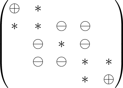 .
.
Figure 4: 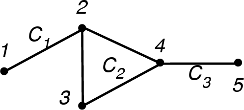 .
.
Here \(\oplus\) denotes a nonnegative real number, \(\ominus\) a nonpositive real number and \(*\) an arbitrary real number. The graph \(G(N,\cal E^0)\) itself is a block-clique graph with \(\hat{p} = 3\) maximal cliques \(C_1= \{1,2\}, C_2 = \{2,3,4\}\) and \(C_3 = \{4,5\}\). The corresponding consistency sets \(\cal D_1 = \{(2,2)\}\), \(\cal D_2 = \{(2,2),(4,4)\}\) and \(\cal D_3 = \{(4,4)\}\) are diagonal. Define \[\begin{align} & & \boldsymbol{A}^p_k = \boldsymbol{A}^{C_p}_k \in \mathbb{S}^{C_p} \;(k=0,1,\ldots,m,p = 1,3), \\ & & \boldsymbol{A}^2_k = \begin{pmatrix}0 & [\boldsymbol{A}_k]_{23} & [\boldsymbol{A}_k]_{24} \\ [\boldsymbol{A}_k]_{32} & [\boldsymbol{A}_k]_{33} & [\boldsymbol{A}_k]_{34} \\ [\boldsymbol{A}_k]_{42} & [\boldsymbol{A}_k]_{43} & 0 \end{pmatrix} \in \mathbb{S}^{C_2} \;(k=0,1,\ldots,m), \end{align}\] so that \(\boldsymbol{A}^p_k\) \((k=0,\ldots,m,p=1,2,3)\) satisfy 3 .
Applying the clique-wise reformulation discussed in Section 2.3 to the SDP relaxation 2 of QCQP 1 , we obtain SDP 7 . The sub-QCQPs on \(C_1\) and \(C_3\) fall into the convex class in Theorem 6, case (I). The sub-QCQP on \(C_2\) falls into the sign-pattern class of Corollary 8, case (i), because all its off-diagonal coefficients are nonpositive. Therefore, for the parameters \(\boldsymbol{\delta}^p\in\mathbb{R}^m\) \((p=1,2,3)\) and the consistency matrix \(\boldsymbol{U}\in \mathbb{S}^n(\overline{\cal D})\) induced by any optimal solution of SDP 7 , all local sub-SDPs are exact. It follows from Theorem 5(iii) that SDP 7 , and consequently SDP 2 , is exact.
This example illustrates that exactness can be preserved even when different local exactness mechanisms are assembled through diagonal consistency constraints.
Example 16. This example illustrates how the local-to-global exactness framework can incorporate three heterogeneous classes of QCQPs with exact SDP relaxations, including a separable sub-QCQP characterized by a limited number of constraints discussed in Theorem 9. The main point of this example is the treatment of the separable sub-QCQP. In contrast to sub-QCQPs characterized by convexity or sign-pattern conditions, the exactness of the associated sub-SDP 14 is parameter-dependent; it depends on the parameters \((\boldsymbol{\delta},\boldsymbol{U})\) induced by the global SDP 7 . We show that suitable conditions on the other sub-SDPs can force the sub-SDP 14 to satisfy Condition (B) of Theorem 9.
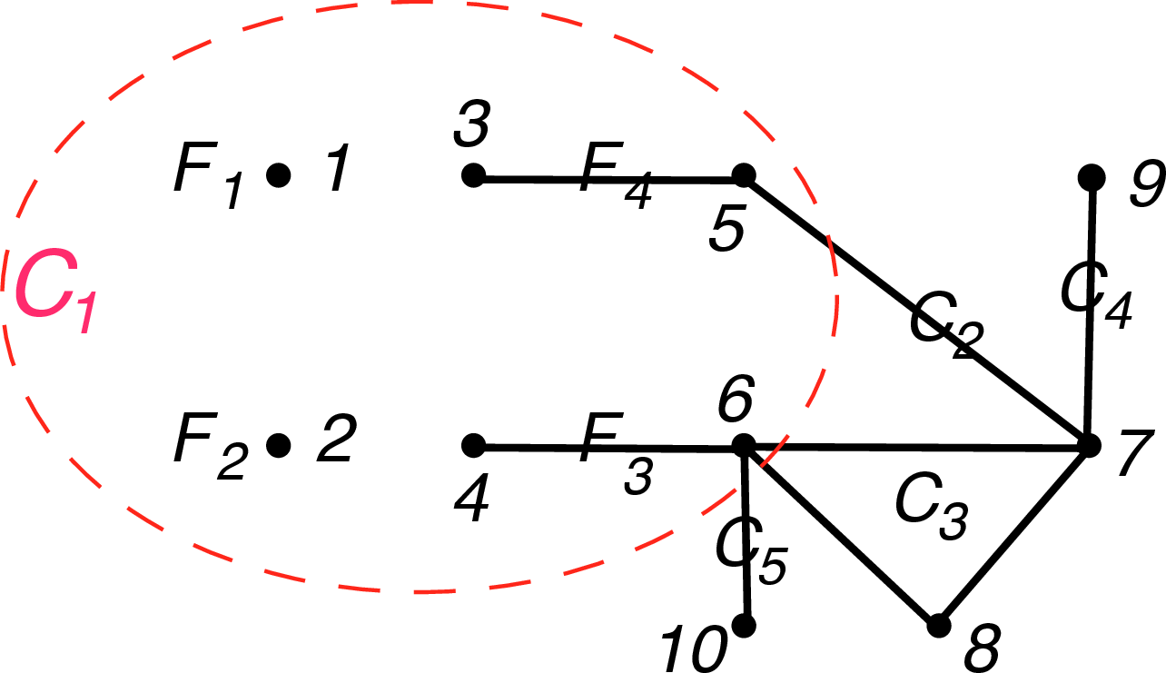
We construct an instance of QCQP 5 by combining five sub-QCQPs on \(C_1=\{1,\ldots,6\}\), \(C_2=\{5,7\},C_3=\{6,7,8\},C_4=\{7,9\}\) and \(C_5=\{6,10\}\). See Figure 3. The clique \(C_1=\{1,\ldots,6\}\) involves four subcliques \(F_1,F_2,F_3,F_4\) of \(G(N,\cal E^0)\), while \(C_2,C_3,C_4,C_5\) are the cliques. We assign a separable QCQP to \(C_1\), QCQPs satisfying sign-pattern conditions to \(C_2\) and \(C_3\), convex QCQPs to \(C_4\) and \(C_5\). Each sub-QCQP has \(m=5\) inequality constraints, including some redundant constraints. Table 1 provides the details of those sub-QCQPs.
| \(p=1: C_1 = \{1,2,3,4,5,6\}\) | \(p=2,3\) | \(p=4,5\) | ||||||||||
| Separable | Sign Pat. | Convex | ||||||||||
| Sect.4.3 | Sect.4.2 | Sect.4.1 | ||||||||||
| \(q=1\) | \(q=2\) | \(q=3\) | \(q=4\) | |||||||||
| \(F_1=\{1\}\) | \(F_2=\{2\}\) | \(F_3=\{3,5\}\) | \(F_4=\{4,6\}\) | \(C_2=\{5,7\}\) | \(C_4=\{7,9\}\) | |||||||
| \(C_3=\{6,7,8\}\) | \(C_5=\{6,10\}\) | |||||||||||
| \(\DC\) | \((5,5)\in\DC_1\) | \((6,6)\in\DC_1\) | \((5,5),(7,7)\in\DC_2\) | \((7,7)\in\DC_4\) | ||||||||
| \((6,6),(7,7)\in\DC_3\) | \((6,6)\in\DC_5\) | |||||||||||
| \(k\) | \(\B_k^1\) | \(\B_k^2\) | \(\B_k^3\) | \(\B_k^4\) | \(\A^2_k\) and \(\A^3_k\) | \(\A^4_k\) and \(\A^5_k\) | \(\trianglelefteq_k\) | \(b_k\) | ||||
| obj. | \(0\) | \(\forall\)sym | \(\forall\)sym | \(\forall\)sym | \(\forall\)sym | off-diag\(\ominus\) | convex | |||||
| \(1\) | \(\forall\)sym | \(\oplus\) | \(\oplus\) | \(\oplus\) | \(\oplus\) & off-diag\(\ominus\) | \(\oplus\) | \(\le\) | \(-\) | ||||
| \(2\) | \(\oplus\) | \(\forall\)sym | \(\oplus\) | \(\oplus\) | \(\oplus\) & off-diag\(\ominus\) | \(\oplus\) | \(\leq\) | \(-\) | ||||
| const. | \(3\) | \(\forall\)sym | \(\forall\)sym | \(\forall\)sym | \(\forall\)sym | off-diag\(\ominus\) | convex | \(\leq\) | \(\forall\) | |||
| \(4\) | \(\O\) | \(\O\) | \(\O\) | \(\O\) | off-diag\(\ominus\) | convex | \(\leq\) | \(\forall\) | ||||
| \(5\) | \(\O\) | \(\O\) | \(\O\) | \(\O\) | off-diag\(\ominus\) | convex | \(\leq\) | \(\forall\) | ||||
For a separable sub-QCQP on \(C_1\), we assume that \(C_1\) consists of \(4\) disjoint cliques \(F_1 = \{1\}, F_2 = \{2\}, F_3=\{3,5\}, F_4=\{4,6\}\) as shown in Figure 3. The sub-QCQP on \(C_1\) contains \(5\) inequality constraints, where the last two constraints, the \(4\)th and \(5\)th constraints are redundant. These two redundant constraints are included solely to match the number \(m=5\) of inequality constraints of the QCQP 5 , which also embeds the sub-QCQPs on \(C_2,\ldots,C_5\). Hence, when applying Theorem 9 to the separable sub-SDP on \(C_1\), we first remove them and use the reduced formulation with the three effective inequalities with \(k=1,2,3\). For Condition (B), we impose \[\begin{align} & & \boldsymbol{A}^{p}_k \in \mathbb{S}^{C_p}_+, \;b_k < 0 \;(p=2,3,4,5,\;k=1,2), \label{eq:Cp}\\ & & \boldsymbol{B}^{q}_1 \in \mathbb{S}^{F_q}_+ \;(q=2,3,4), \; \boldsymbol{B}^{q}_2 \in \mathbb{S}^{F_q}_+ \;(q=1,3,4). \label{eq:Fq} \end{align}\] {#eq: sublabel=eq:eq:Cp,eq:eq:Fq} The condition ?? ensures that, for every optimal solution \((\boldsymbol{Y}^1,\ldots,\boldsymbol{Y}^5,\boldsymbol{U})\) of SDP 7 , \[\begin{align} \delta^1_k = \langle\boldsymbol{A}^{1}_k, \, \boldsymbol{Y}^1\rangle \le b_k - \sum_{p=2}^5 \langle\boldsymbol{A}^{p}_k, \, \boldsymbol{Y}^p\rangle < 0 \;(k=1,2). \end{align}\] Then the condition ?? ensures that \(\boldsymbol{W}^1 \ne \boldsymbol{O}\) and \(\boldsymbol{W}^2 \ne \boldsymbol{O}\) for every optimal solution \((\boldsymbol{W}^1,\ldots,\boldsymbol{W}^4)\) of the separable SDP 14 for these \(\delta^1_1 < 0\), \(\delta^1_2<0\) and any \(\delta^1_3 \in \mathbb{R}\).
If both \(U_{55}\) and \(U_{66}\) are positive, then \(\mu=2\) in the reduced separable sub-SDP. Since the reduced formulation has three effective inequality constraints, Condition (B) requires \(3+\mu-1=4\) nonzero elements. The conditions above imply \(\boldsymbol{W}^1\ne\boldsymbol{O}\) and \(\boldsymbol{W}^2\ne\boldsymbol{O}\), while \(U_{55}>0\) and \(U_{66}>0\) imply \(\boldsymbol{W}^3\ne\boldsymbol{O}\) and \(\boldsymbol{W}^4\ne\boldsymbol{O}\). Hence Condition (B) is satisfied.
If \(U_{55}=0\) and/or \(U_{66}=0\), the corresponding row and column can be eliminated by positive semidefiniteness, as described in Theorem 9. The number \(\mu\) decreases accordingly, and the required number of nonzero elements in Condition (B) decreases by the same amount. Therefore, the reduced separable sub-SDP on \(C_1\) is exact.
For the sub-QCQPs on \(C_2\) and \(C_3\), we impose the sign-pattern conditions. Specifically, all off-diagonal elements of \(\boldsymbol{A}^{p}_k\) \((k=0,\ldots,5,\;p=2,3)\) are assumed to be nonpositive. By Corollary 8(i), the corresponding sub-SDPs are exact for every \(\boldsymbol{\delta}\in\mathbb{R}^m\) and \(\boldsymbol{U}\). In addition, to ensure that the separable sub-QCQP on \(C_1\) satisfies Condition (B), we have assumed that \(\boldsymbol{A}^{p}_k \in \mathbb{S}^{C_p}_+\) \((k=1,2,p=2,3)\).
For the sub-QCQPs on \(C_4\) and \(C_5\), we use the convex QCQPs discussed in Section 4.1. Since \(\cal D_4=\{(i_4,i_4)\}=\{(7,7)\}\) and \(\cal D_5=\{(i_5,i_5)\}=\{(6,6)\}\), case (I) of Theorem 6 applies to both sub-QCQPs. Thus, we impose the convexity condition that the principal submatrix of \(\boldsymbol{A}^p_k\) indexed by \(C_p\backslash\{i_p\}\) is positive semidefinite \((k=0,\ldots,5,p=4,5)\), or equivalently, \([\boldsymbol{A}^4_k]_{99} \geq 0, \;[\boldsymbol{A}^5_k]_{10,10} \geq 0 \;(k=0,\ldots,5).\) It follows that the sub-SDPs 13 on \(C_4\) and \(C_5\) are exact for every \(\boldsymbol{\delta}\in\mathbb{R}^m\) and \(\boldsymbol{U}\). In order for the separable sub-QCQP on \(C_1\) to satisfy Condition (B), we have assumed that \(\boldsymbol{A}^{p}_k \in \mathbb{S}^{C_p}_+\) \((k=1,2,p=4,5)\).
Consequently, each local sub-SDP induced by an optimal solution of SDP 7 is exact. It follows from Theorem 5(iii) that SDP 7 , and therefore SDP 2 , is exact. This example highlights a feature that does not arise in the purely convex or sign-pattern cases: the exactness of one local sub-SDP may be certified using parameter information imposed by the other local sub-SDPs through the global constraints.
6 Concluding remarks↩︎
We have developed a local-to-global exactness framework for SDP relaxations of sparse QCQPs. Using a chordal extension of the aggregate sparsity pattern graph, the SDP relaxation is reformulated in clique-wise matrix variables associated with the maximal cliques. This equivalent reformulation induces local sub-SDPs linked by consistency constraints on clique overlaps. The main result shows that exactness of the original SDP relaxation can be certified by rank-at-most-one attainability of the local sub-SDPs with the local right-hand-side vectors and consistency matrix induced by an optimal solution of the clique-wise formulation.
For the applications developed in this paper, the block-clique assumption is imposed in handling the consistency of rank-at-most-one optimal solutions of the local sub-SDPs. Under this assumption, all consistency constraints on clique overlaps are diagonal, so local rank-at-most-one optimal solutions can be combined without imposing additional off-diagonal rank-one consistency conditions. This allows different local exactness mechanisms to be used within a single sparse QCQP. In particular, we have identified three mechanisms based, respectively on convexity, sign-pattern conditions, and separability with a limited number of constraints. The examples in Section 5 illustrate how these heterogeneous local exactness mechanisms can be assembled to prove exactness of the original SDP relaxation.
An important issue for future work is the choice of chordal extension and clique-wise decomposition of the data matrices. Different chordal extensions, and different decompositions over their maximal cliques, may lead to different local sub-SDPs. Consequently, they may affect whether the local exactness certificates developed in this paper can be applied.
It would also be valuable to further enlarge the list of local sub-QCQP classes with exact SDP relaxations. The framework is modular: any new local exactness result that is stable under the induced right-hand side and consistency matrix can be incorporated into the global certification scheme. This suggests that sparse exactness analysis may serve as a way to combine otherwise separate exactness criteria for nonconvex QCQPs.