Harmonic basis vector fields on surfaces
June 19, 2026
Abstract
In this paper, we study local parameterizations of surfaces in the Euclidean space \(\mathbb{R}^3\) whose coordinate vector fields are harmonic sections with respect to the induced Riemannian metric. After introducing
the notion of harmonic basis vector fields on a surface, we derive necessary and sufficient conditions under which the coordinate vector fields \(\frac{\partial}{\partial u}\) and \(\frac{\partial}{\partial v}\) are harmonic. We then focus on two important classes of surfaces: surfaces of revolution and translation surfaces. For these families, we obtain a complete classification of all parameterizations
admitting harmonic basis vector fields.
Keywords: Harmonic maps, Harmonic vector fields
MSC 2020: 58E20, 53C12.
1 Introduction↩︎
The study of harmonic objects on Riemannian manifolds has been a fundamental topic in differential geometry and geometric analysis for many decades. A smooth map \(\varphi:(M,g)\longrightarrow(N,h)\) between two
Riemannian manifolds has the energy on a compact domain \(D\) of \(M\), defined by \[\label{eq1461}
E(\varphi;D)=\frac{1}{2}\int_D|d\varphi|^2 v^g,\tag{1}\] where \(v^g\) is the volume element on \((M,g)\), and \(|d\varphi|\) is the
Hilbert-Schmidt norm of the differential \(d\varphi\). If \(\varphi\) is a critical point of the energy functional (1 ), then the map is referred to as harmonic. We
have \(\tau(\varphi)=\operatorname{Tr}_g\nabla d\varphi=0\) as the Euler Lagrange equation for (1 ), where \(\nabla d\varphi\) is the second fundamental form of the
smooth map \(\varphi\) (see [1], [2]).
The systematic study of harmonic vector fields was initiated by Wood [3] and later developed by several authors. Let \((TM, g_S)\)
the tangent bundle of a Riemanian manifold \((M, g)\) equipped with the Sasaki metric \(g_S\) defined by \[g_S(X^h,Y^h)=g_S(X^v,Y^v)=g(X,Y)\circ\pi,\quad
g_S(X^h,Y^v)=0,\] for all \(X,Y\in\Gamma(TM)\), where \(\pi:TM\longrightarrow M\) is the natural projection, and \(X^h\) (resp. \(X^v\)) the horizontal (resp. vertical) lift of a vector field \(X\) on \(M\) to \(TM\) (see [4]).
In [5], the author proves that the tension field of \(X:(M,g)\longrightarrow(TM,g_S)\) is given by
\[\label{eq14624242}
\tau(X)=(\operatorname{Tr}_gR(X,\nabla_\cdot X)\cdot)^h+(\operatorname{Tr}_g\nabla^2X)^v.\tag{2}\] Therfore, \(X:(M,g)\longrightarrow(TM,g_S)\) is harmonic map if and only if \[\operatorname{Tr}_gR(X,\nabla_\cdot X)\cdot=0,\quad\operatorname{Tr}_g\nabla^2X=0,\] where \(R\) is the Riemannian curvature of \((M,g)\). Important
contributions include the investigation of harmonic sections of tangent bundles [4], the relationship between volume and energy of vector fields [5], and the total bending of vector fields on Riemannian manifolds [6]. Further results
concerning existence and classification of harmonic vector fields can be found in [7].
A smooth vector field \(X\) on \((M,g)\) is said to be a harmonic section if it is a critical point of the vertical energy \[\label{eq1463} E^v(X;D)=\frac{1}{2}\int_D|\nabla X|^2 v^g.\tag{3}\] The corresponding Euler-Lagrange equation is given by \(\overline{\Delta}X=\operatorname{Tr}_g\nabla^2X=0\).
Harmonic vector fields represent an important class characterized by their minimization of energy and their connection to both geometric analysis. In this work, we present a new classification of harmonic vector fields on surfaces. Specifically, we begin
by introducing a class of parameterizations whose basis vector fields are harmonic when viewed as sections of the tangent bundle.
Let \(M^2\) be a surface in the Euclidean space \(\mathbb{R}^3\). We say that a local parameterization \[\phi: (u,v) \longmapsto (x(u,v), y(u,v), z(u,v)),\]
of \(M^2\) has harmonic basis vector fields if \(\frac{\partial}{\partial u}\) and \(\frac{\partial}{\partial v}\) are harmonic sections on \((M^2,g)\), where \(g\) is the induce Riemannian metric.
A fundamental theme in this area is the appearance of Liouville-type theorems, which assert the nonexistence of nontrivial harmonic objects under suitable geometric or analytic conditions. Recently, in [8], the author established several Liouville-type theorems for harmonic and biharmonic maps. These results naturally motivate the study of analogous rigidity phenomena for harmonic vector fields.
In this work, we focus on harmonic basis vector fields associated with local coordinate systems on Riemannian surfaces. As a concrete and geometrically rich class of examples, we consider translation surfaces and surfaces of revolution in \(\mathbb{R}^3\). These surfaces admit natural coordinate systems, making them particularly suitable for the study of harmonic coordinate vector fields. By computing explicitly the rough Laplacian of the basis vector fields, we
derive necessary and sufficient conditions for their harmonicity. More precisely, we prove that a surface of revolution whose coordinate vector fields are harmonic must have zero Gaussian curvature. As a consequence, such surfaces are necessarily planes,
cylinders, or cones. This classification result may be viewed as a Liouville-type theorem for harmonic basis vector fields on surfaces of revolution, in the spirit of the rigidity results obtained for harmonic maps in [8]. In particular, we show that harmonic sections coincide with harmonic maps. As an application, we prove that for translation surfaces this condition characterizes either planar
surfaces or a specific nontrivial family described by explicit functions.
2 Harmonic basis vector fields on translation surfaces↩︎
A translation surface is a surface defined by the following parametric representation \[\begin{align} \phi: I \times J \subset \mathbb{R}^2 &\longrightarrow \mathbb{R}^3, \\ (u,v) &\longmapsto \phi(u,v) = \alpha(u) + \beta(v) \end{align}\] where \(\alpha\) and \(\beta\) are two smooth curves in \(\mathbb{R}^3\), of class \(C^{\infty}\), defined on open intervals \(I\) and \(J\), respectively. A well-known class of translation surfaces is generated by two planar curves that lie in orthogonal planes. This special case is referred to as a translation surface of plane type, and it takes the form \[\begin{align} \phi(u,v) = (u, v, f(u) + h(v)), \label{translation-surface} \end{align}\tag{4}\] where \(f\) and \(h\) are smooth real-valued functions defined on \(I\) and \(J\), respectively. The basic vector fields associated with the translation surface translation-surface are given by \[\label{eq2461} \frac{\partial}{\partial u} = \phi_u = (1, 0, f'), \quad \frac{\partial}{\partial v} = \phi_v = (0, 1, h').\tag{5}\] The unit normal vector field of the surface is computed as \[\begin{align} \label{eq2462} \mathbf{N} &= \frac{\phi_u \wedge \phi_v}{\|\phi_u \wedge \phi_v\|} = \frac{1}{\sqrt{1 + f'^2 + h'^2}}\,(-f', -h', 1). \end{align}\tag{6}\] The coefficients of the first fundamental form are given by \[\begin{align} E &= \langle \phi_u, \phi_u \rangle = 1 + f'^2, \\ F &= \langle \phi_u, \phi_v \rangle = f' h', \\ G &= \langle \phi_v, \phi_v \rangle = 1 + h'^2. \end{align}\] Thus, the induced Riemannian metric takes the form \[\begin{align} \label{eq2463} g &= E\,du^2 + 2F\,du\,dv + G\,dv^2 \nonumber\\ &= (1 + f'^2)\,du^2 + 2f'h'\,du\,dv + (1 + h'^2)\,dv^2. \end{align}\tag{7}\] The second-order partial derivatives of the parametrization are \[\begin{align} \phi_{uu} &= (0, 0, f''), \\ \phi_{uv} &= (0, 0, 0), \\ \phi_{vv} &= (0, 0, h''). \end{align}\] The coefficients of the second fundamental form are then given by \[\begin{align} L &= \langle \mathbf{N}, \phi_{uu} \rangle = \frac{f''}{\sqrt{1 + f'^2 + h'^2}}, \\ M &= \langle \mathbf{N}, \phi_{uv} \rangle = 0, \\ N &= \langle \mathbf{N}, \phi_{vv} \rangle = \frac{h''}{\sqrt{1 + f'^2 + h'^2}}. \end{align}\] Hence, the second fundamental form is \[\label{eq2464} \mathrm{II} = \frac{f''}{\sqrt{1 + f'^2 + h'^2}}\,du^2 + \frac{h''}{\sqrt{1 + f'^2 + h'^2}}\,dv^2.\tag{8}\] The Gaussian curvature \(\mathbf{K}\) and the mean curvature \(\mathbf{H}\) of the surface are given by \[\begin{align} \mathbf{K} &= \frac{LN - M^2}{EG - F^2} = \frac{f'' h''}{(1 + f'^2 + h'^2)^2},\tag{9} \\ \mathbf{H} &= \frac{GL + EN - 2FM}{2(EG - F^2)} = \frac{f''(1 + h'^2) + h''(1 + f'^2)}{2(1 + f'^2 + h'^2)^{\frac{3}{2}}}.\tag{10} \end{align}\] The non-zero Christoffel symbols \(\Gamma_{ij}^k\) of the surface are given by \[\begin{align} \Gamma_{11}^1 &= \frac{f' f''}{1 + f'^2 + h'^2}, \quad & \Gamma_{11}^2 &= \frac{h' f''}{1 + f'^2 + h'^2}, \\ \Gamma_{22}^1 &= \frac{f' h''}{1 + f'^2 + h'^2}, \quad & \Gamma_{22}^2 &= \frac{h' h''}{1 + f'^2 + h'^2}. \end{align}\] We define the following orthonormal basic vector fields \[e_1=\frac{1}{\sigma_2}\;\frac{\partial}{\partial u},\qquad e_2=-\frac{f'h'}{\sigma_1 \sigma_2}\;\frac{\partial}{\partial u}+\frac{\sigma_2}{\sigma_1}\;\frac{\partial}{\partial v},\] where \(\sigma_1=\sigma_1(u,v)=\sqrt{1+f{'}^2+h{'}^2}\) and \(\sigma_2=\sigma_2(u)=\sqrt{1+f{'}^2}\). By using the Christoffel symbols formulas, we have the following \[\label{eq2467} \nabla_{e_1}e_1=-\frac{f'f''h{'}^2}{\sigma_1^2\sigma_2^4}\frac{\partial}{\partial u}+\frac{h'f''}{\sigma_1^2\sigma_2^2}\frac{\partial}{\partial v} ,\quad \nabla_{e_2}e_2=\frac{f'h{'}^2f''}{\sigma_1^2\sigma_2^4}\frac{\partial}{\partial u}.\tag{11}\]
By explicitly computing the rough Laplacian of these vector fields with respect to the Levi-Civita connection of \(g\), we obtain a system of nonlinear ordinary differential equations involving the functions \(f\) and \(h\). The following theorem provides necessary and sufficient conditions for the harmonicity of the coordinate vector fields in terms of this system.
Theorem 1. The basis vectors fields \(\frac{\partial}{\partial u}\) and \(\frac{\partial}{\partial v}\) given in (5 ) are harmonic sections on \((M^2,g)\) if and only if \[{\normalsize (S_1)\,\begin{cases} f{''}^2\left(1+h{'}^2\right)\left(1+h{'}^2-f{'}^2\right)+f{'}f{'''}\left(1+h{'}^2\right)\left(1+h{'}^2+f{'}^2\right) -f{'}^2f{''}h{''}\left(1+f{'}^2-h{'}^2\right)=0, \\ h{'}\left[ f{'''}\left(1+h{'}^2\right)\left(1+f{'}^2+h{'}^2\right)-2f{'}f{''}\left(h{''}\left(1+f{'}^2\right) +f{''}\left(1+h{'}^2\right)\right)\right]=0, \\ f{'}\left[h{'''}\left(1+f{'}^2\right)\left(1+f{'}^2+h{'}^2\right)-2h{'}h{''}\left(f{''}\left(1+h{'}^2\right) +h{''}\left(1+f{'}^2\right)\right)\right]=0,\\ h{''}^2\left(1+f{'}^2\right)\left(1+f{'}^2-h{'}^2\right)+h{'}h{'''}\left(1+f{'}^2\right)\left(1+f{'}^2+h{'}^2\right) -h{'}^2h{''}f{''}\left(1+h{'}^2-f{'}^2\right)=0. \end{cases}}\]
Proof. First, we compute the Laplacian of \(\frac{\partial}{\partial u}\). We have \[\label{eq2468} \Delta\left(\frac{\partial}{\partial u}\right)=\nabla_{e_1}\nabla_{e_1}\frac{\partial}{\partial u}-\nabla_{\nabla_{e_1}e_1}\frac{\partial}{\partial u}+\nabla_{e_2}\nabla_{e_2}\frac{\partial}{\partial u}-\nabla_{\nabla_{e_2}e_2}\frac{\partial}{\partial u}.\tag{12}\] We compute \(\nabla_{\nabla_{e_1}e_1}\frac{\partial}{\partial u}\) and \(\nabla_{\nabla_{e_2}e_2}\frac{\partial}{\partial u}\). By using the formulas (11 ), we get \[\begin{align} \nabla_{\nabla_{e_1}e_1}\frac{\partial}{\partial u} &=\nabla_{\left(-\frac{f'f''h{'}^2}{\sigma_2^4\sigma_1^2}\frac{\partial}{\partial u} +\frac{h'f''}{\sigma_1^2\sigma_2^2}\frac{\partial}{\partial v}\right)}\frac{\partial}{\partial u}\\ &=-\frac{f'f''h{'}^2}{\sigma_2^4\sigma_1^2} \nabla_{\frac{\partial}{\partial u}}\frac{\partial}{\partial u} +\frac{h'f''}{\sigma_1^2\sigma_2^2}\nabla_{\frac{\partial}{\partial v}}\frac{\partial}{\partial u}\\ &=-\frac{f'f''h{'}^2}{\sigma_2^4\sigma_1^2}\left(\frac{f'f''}{\sigma_1^2}\frac{\partial}{\partial u} +\frac{h'f''}{\sigma_1^2}\frac{\partial}{\partial v}\right)\\ &=-\frac{f{'}^2f{''}^2h{'}^2}{\sigma_1^4\sigma_2^4}\frac{\partial}{\partial u} -\frac{f{'}f{''}^2h{'}^3}{\sigma_1^4\sigma_2^4}\frac{\partial}{\partial v}, \end{align}\] and the following \[\begin{align} \nabla_{\nabla_{e_2}e_2}\frac{\partial}{\partial u}&=\nabla_{\frac{f'f''h{'}^2}{\sigma_1^2\sigma_2^4}\frac{\partial}{\partial u}}\frac{\partial}{\partial u}\\ &=\frac{f'f''h{'}^2}{\sigma_1^2\sigma_2^4}\nabla_{\frac{\partial}{\partial u}}\frac{\partial}{\partial u}\\ &=\frac{f'f''h{'}^2}{\sigma_1^2\sigma_2^4}\left(\frac{f'f''}{\sigma_1^2}\frac{\partial}{\partial u}+\frac{h'f''}{\sigma_1^2} \frac{\partial}{\partial v}\right)\\ &=\frac{f{'}^2f{''}^2h{'}^2}{\sigma_1^4\sigma_2^4}\frac{\partial}{\partial u}+\frac{f{'}f{''}^2h{'}^3}{\sigma_1^4\sigma_2^4}\frac{\partial}{\partial v}. \end{align}\] Note that, \(\nabla_{\nabla_{e_2}e_2}\frac{\partial}{\partial u}=- \nabla_{\nabla_{e_1}e_1}\frac{\partial}{\partial u}\). We compute \(\nabla_{e_1}\nabla_{e_1}\frac{\partial}{\partial u}\) and \(\nabla_{e_2}\nabla_{e_2}\frac{\partial}{\partial u}\). We have \[\begin{align} \nabla_{e_1}\frac{\partial}{\partial u}&= \nabla_{\frac{1}{\sigma_2}\frac{\partial}{\partial u}}\frac{\partial}{\partial u}\\ &=\frac{1}{\sigma_2}\left(\frac{f'f''}{\sigma_1^2}\frac{\partial}{\partial u}+\frac{h'f''}{\sigma_1^2} \frac{\partial}{\partial v}\right)\\ &=\frac{f'f''}{\sigma_1^2\sigma_2}\frac{\partial}{\partial u}+\frac{h'f''}{\sigma_1^2\sigma_2} \frac{\partial}{\partial v}, \end{align}\] and the following \[\begin{align} \nabla_{e_2}\frac{\partial}{\partial u}&= \nabla_{-\frac{f'h'}{\sigma_1 \sigma_2}\;\frac{\partial}{\partial u}+\frac{\sigma_2}{\sigma_1}\;\frac{\partial}{\partial v}}\frac{\partial}{\partial u}\\ &=-\frac{f'h'}{\sigma_1 \sigma_2}\nabla_{\frac{\partial}{\partial u}}\frac{\partial}{\partial u}+\frac{\sigma_2}{\sigma_1}\nabla_{\frac{\partial}{\partial v}}\frac{\partial}{\partial u}\\ &=-\frac{f'h'}{\sigma_1 \sigma_2}\left(\frac{f'f''}{\sigma_1^2}\frac{\partial}{\partial u}+\frac{h'f''}{\sigma_1^2} \frac{\partial}{\partial v}\right)\\ &=-\frac{f{'}^2f''h'}{\sigma_1^3\sigma_2}\frac{\partial}{\partial u}-\frac{f'f''h{'}^2}{\sigma_1^3\sigma_2}\frac{\partial}{\partial v}. \end{align}\] Therefore, the term \(\nabla_{e_1}\nabla_{e_1}\frac{\partial}{\partial u}\) is given by \[\begin{align} \nabla_{e_1}\nabla_{e_1}\frac{\partial}{\partial u}&=\nabla_{\frac{1}{\sigma_2}\frac{\partial}{\partial u}}\left(\frac{f'f''}{\sigma_1^2\sigma_2}\frac{\partial}{\partial u}+\frac{h'f''}{\sigma_1^2\sigma_2} \frac{\partial}{\partial v}\right)\\ &=\frac{1}{\sigma_2}\left(\frac{\partial}{\partial u}\left(\frac{f'f''}{\sigma_1^2\sigma_2}\right)\frac{\partial}{\partial u}+\frac{f'f''}{\sigma_1^2\sigma_2}\nabla_{\frac{\partial}{\partial u}}\frac{\partial}{\partial u}+\frac{\partial}{\partial u}\left(\frac{h'f''}{\sigma_1^2\sigma_2}\right)\frac{\partial}{\partial v}+\frac{h'f''}{\sigma_1^2\sigma_2}\nabla_{\frac{\partial}{\partial u}}\frac{\partial}{\partial v}\right)\\ &=\frac{1}{\sigma_2}\left(\frac{f{''}^2\sigma_1^2+f'f'''\sigma_1^2\sigma_2^2-2f{'}^2f{''}^2\sigma_2^2}{\sigma_1^4\sigma_2^3}\frac{\partial}{\partial u}+\frac{f'f''}{\sigma_1^2\sigma_2}\left(\frac{f'f''}{\sigma_1^2}\frac{\partial}{\partial u}+\frac{h'f''}{\sigma_1^2}\frac{\partial}{\partial v}\right)\right. \notag\\ &\quad \left.+\frac{f'''h'\sigma_1^2\sigma_2^2-f'f{''}^2h'\sigma_1^2-2f'f{''}^2h'\sigma_2^2}{\sigma_1^4\sigma_2^3}\frac{\partial}{\partial v}\right)\\ &=\frac{1}{\sigma_2}\left(\frac{f{''}^2\sigma_1^2+f'f'''\sigma_1^2\sigma_2^2-2f{'}^2f{''}^2\sigma_2^2}{\sigma_1^4\sigma_2^3}\frac{\partial}{\partial u}+\frac{f{'}^2f{''}^2\sigma_2^2}{\sigma_1^4\sigma_2^3}\frac{\partial}{\partial u}+\frac{f'f{''}^2h'\sigma_2^2}{\sigma_1^4\sigma_2^3}\frac{\partial}{\partial v}\right. \notag\\ &\quad \left.+\frac{f'''h'\sigma_1^2\sigma_2^2-f'f{''}^2h'\sigma_1^2-2f'f{''}^2h'\sigma_2^2}{\sigma_1^4\sigma_2^3}\frac{\partial}{\partial v}\right)\\ &=\frac{f{''}^2\sigma_1^2+f'f'''\sigma_1^2\sigma_2^2-f{'}^2f{''}^2\sigma_2^2}{\sigma_1^4\sigma_2^4}\frac{\partial}{\partial u}+\frac{f'''h'\sigma_1^2\sigma_2^2-f'f{''}^2h'\sigma_1^2-f'f{''}^2h'\sigma_2^2}{\sigma_1^4\sigma_2^4}\frac{\partial}{\partial v}, \end{align}\] and the term \(\nabla_{e_2}\nabla_{e_2}\frac{\partial}{\partial u}\) is given by \[\begin{align} \nabla_{e_2}\nabla_{e_2}\frac{\partial}{\partial u}&=\nabla_{ -\frac{f'h'}{\sigma_1 \sigma_2}\;\frac{\partial}{\partial u}+\frac{\sigma_2}{\sigma_1}\;\frac{\partial}{\partial v}}\left(-\frac{f{'}^2f''h'}{\sigma_1^3\sigma_2}\frac{\partial}{\partial u}-\frac{f'f''h{'}^2}{\sigma_1^3\sigma_2}\frac{\partial}{\partial v}\right)\\ &=-\frac{f'h'}{\sigma_1 \sigma_2}\nabla_{\frac{\partial}{\partial u}}\left(-\frac{f{'}^2f''h'}{\sigma_1^3\sigma_2}\frac{\partial}{\partial u}-\frac{f'f''h{'}^2}{\sigma_1^3\sigma_2}\frac{\partial}{\partial v}\right)\notag\\ &\quad +\frac{\sigma_2}{\sigma_1}\nabla_{\frac{\partial}{\partial v}}\left(-\frac{f{'}^2f''h'}{\sigma_1^3\sigma_2}\frac{\partial}{\partial u}-\frac{f'f''h{'}^2}{\sigma_1^3\sigma_2}\frac{\partial}{\partial v}\right)\\ &=-\frac{f'h'}{\sigma_1 \sigma_2}\left(-\frac{\partial}{\partial u}\left(\frac{f{'}^2f''h'}{\sigma_1^3\sigma_2}\right)\frac{\partial}{\partial u}-\frac{f{'}^2f''h'}{\sigma_1^3\sigma_2}\nabla_{\frac{\partial}{\partial u}}\frac{\partial}{\partial u}-\frac{\partial}{\partial u}\left(\frac{f{'}f''h{'}^2}{\sigma_1^3\sigma_2}\right)\frac{\partial}{\partial v}\right)\notag\\ &\quad +\frac{\sigma_2}{\sigma_1}\left(-\frac{\partial}{\partial v}\left(\frac{f{'}^2f''h'}{\sigma_1^3\sigma_2}\right)\frac{\partial}{\partial u}-\frac{\partial}{\partial v}\left(\frac{f{'}f''h{'}^2}{\sigma_1^3\sigma_2}\right)\frac{\partial}{\partial v}-\frac{f{'}f''h{'}^2}{\sigma_1^3\sigma_2}\nabla_{\frac{\partial}{\partial v}}\frac{\partial}{\partial v}\right)\\ &=-\frac{f'h'}{\sigma_1 \sigma_2}\left(\frac{-2f'h'f{''}^2\sigma_1^2\sigma_2^2-f{'}^2f'''h'\sigma_1^2\sigma_2^2+3f{'}^3f{''}^2h'\sigma_2^2+f{'}^3f{''}^2h'\sigma_1^2}{\sigma_1^5\sigma_2^3}\frac{\partial}{\partial u}\right.\notag\\ &\quad \left.-\frac{f{'}^2f''h'}{\sigma_1^3\sigma_2}\left(\frac{f'f''}{\sigma_1^2}\frac{\partial}{\partial u}+\frac{f''h'}{\sigma_1^2}\frac{\partial}{\partial v}\right)\right.\notag\\ &\quad \left.+\frac{-f{''}^2h{'}^2\sigma_1^2-f'f'''h{'}^2\sigma_1^2\sigma_2^2+3f{'}^2f{''}^2h{'}^2\sigma_2^2}{\sigma_1^5\sigma_2^3}\frac{\partial}{\partial v}\right)\notag\\ &\quad +\frac{\sigma_2}{\sigma_1}\left(\frac{-f{'}^2f''h''\sigma_1^2+3f{'}^2f''h{'}^2h''}{\sigma_1^5\sigma_2}\frac{\partial}{\partial u}+\frac{-2f'f''h'h''\sigma_1^2+3f'f''h{'}^3h''}{\sigma_1^5\sigma_2}\frac{\partial}{\partial v}\right.\notag\\ &\quad \left.-\frac{f'f''h{'}^2}{\sigma_1^3\sigma_2}\left(\frac{f'h''}{\sigma_1^2}\frac{\partial}{\partial u}+\frac{h'h''}{\sigma_1^2}\frac{\partial}{\partial v}\right)\right)\\ &=\frac{1}{\sigma_1^6\sigma_2^4}\left(2f{'}^2f{''}^2h{'}^2\sigma_1^2\sigma_2^2+f{'}^3f'''h{'}^2\sigma_1^2\sigma_2^2-2f{'}^4f{''}^2h{'}^2\sigma_2^2-f{'}^4f{''}^2h{'}^2\sigma_1^2\right.\notag\\ &\quad \left.-f{'}^2f''h''\sigma_1^2\sigma_2^4+2f{'}^2f''h{'}^2h''\sigma_2^4\right)\frac{\partial}{\partial u}\notag\\ &\quad +\frac{1}{\sigma_1^6\sigma_2^4} \left(f'f{''}^2h{'}^3\sigma_1^2+f{'}^2f'''h{'}^3\sigma_1^2\sigma_2^2-2f{'}^3f{''}^2h{'}^3\sigma_2^2-2f'f''h'h''\sigma_1^2\sigma_2^4\right.\notag\\ &\quad \left.+2f'f''h{'}^3h''\sigma_2^4\right)\frac{\partial}{\partial v}. \end{align}\] Replacing these formulas into (12 ), we obtain \[\begin{align} \Delta\left(\frac{\partial}{\partial u}\right)&=\nabla_{e_1}\nabla_{e_1}\frac{\partial}{\partial u}+\nabla_{e_2}\nabla_{e_2}\frac{\partial}{\partial u}\\ &=\frac{1}{\sigma_1^6\sigma_2^4}\left(f{''}^2\sigma_1^4+f'f'''\sigma_1^4\sigma_2^2-f{'}^2f{''}^2\sigma_1^2\sigma_2^2+2f{'}^2f{''}^2h{'}^2\sigma_1^2\sigma_2^2\right.\notag\\ &\quad \left.+f{'}^3f'''h{'}^2\sigma_1^2\sigma_2^2-2f{'}^4f{''}^2h{'}^2\sigma_2^2-f{'}^4f{''}^2h{'}^2\sigma_1^2-f{'}^2f''h''\sigma_1^2\sigma_2^4\right.\notag\\ &\quad \left.+2f{'}^2f''h{'}^2h''\sigma_2^4\right)\frac{\partial}{\partial u} \notag\\ &\quad +\frac{1}{\sigma_1^6\sigma_2^4}\left(f'''h'\sigma_1^4\sigma_2^2-f'f{''}^2h'\sigma_1^4-f'f{''}^2h'\sigma_1^2\sigma_2^2+f'f{''}^2h{'}^3\sigma_1^2\right.\notag\\ &\quad \left.+f{'}^2f'''h{'}^3\sigma_1^2\sigma_2^2-2f{'}^3f{''}^2h{'}^3\sigma_2^2-2f'f''h'h''\sigma_1^2\sigma_2^4\right.\notag\\ &\quad \left.+2f'f''h{'}^3h''\sigma_2^4\right)\frac{\partial}{\partial v}\\ &=\frac{1}{\sigma_1^6}\left(-f{'}^4f''h''+f{'}^3f'''h{'}^2+f{'}^3f'''+f{'}^2f''h{'}^2h''-f{'}^2f{''}^2-f{'}^2f{''}^2h{'}^2\right.\notag\\ &\quad \left.-f{'}^2f''h''+f'f'''h{'}^4+2f'f'''h{'}^2+f'f'''+f{''}^2+2f{''}^2h{'}^2+f{''}^2h{'}^4\right)\frac{\partial}{\partial u} \notag\\ &\quad+\frac{h'}{\sigma_1^6} \left(-2f{'}^3f''h''+f{'}^2f'''h{'}^2+f{'}^2f'''-2f'f{''}^2-2f'f{''}^2h{'}^2-2f'f''h''\right.\notag\\ &\quad \left.+f'''h{'}^4+2f'''h{'}^2+f'''\right)\frac{\partial}{\partial v}\\ &=\frac{1}{\sigma_1^6} \left(f{''}^2\left(1+h{'}^2\right)\left(1+h{'}^2-f{'}^2\right)+f{'}f{'''}\left(1+h{'}^2\right)\left(1+h{'}^2+f{'}^2\right)\right.\notag\\ &\quad \left.-f{'}^2f{''}h{''}\left(1-h{'}^2+f{'}^2\right)\right)\frac{\partial}{\partial u}\notag\\ &\quad +\frac{h{'}}{\sigma_1^6}\left(f{'''}\left(1+h{'}^2\right)\left(1+h{'}^2+f{'}^2\right) -2f{'}f{''}\left[h{''}\left(1+f{'}^2\right)+f{''}\left(1+h{'}^2\right)\right]\right)\frac{\partial}{\partial v}. \end{align}\] We compute now \(\Delta\left(\frac{\partial}{\partial v}\right)\). We have \[\label{eq2469} \Delta\left(\frac{\partial}{\partial v}\right)=\nabla_{e_1}\nabla_{e_1}\frac{\partial}{\partial v}-\nabla_{\nabla_{e_1}e_1}\frac{\partial}{\partial v}+\nabla_{e_2}\nabla_{e_2}\frac{\partial}{\partial v}-\nabla_{\nabla_{e_2}e_2}\frac{\partial}{\partial v}.\tag{13}\] Calculate \(\nabla_{\nabla_{e_1}e_1}\frac{\partial}{\partial v}\) and \(\nabla_{\nabla_{e_2}e_2}\frac{\partial}{\partial v}\). By using the formulas (11 ), we find that \[\begin{align} \nabla_{\nabla_{e_1}e_1}\frac{\partial}{\partial v}&=\nabla_{\left(\frac{-f'f''h{'}^2}{\sigma_1^2\sigma_2^4}\frac{\partial}{\partial u}+\frac{f''h'}{\sigma_1^2\sigma_2^2}\frac{\partial}{\partial v}\right)}\frac{\partial}{\partial v}\\ &=\frac{f''h'}{\sigma_1^2\sigma_2^2}\nabla_{\frac{\partial}{\partial v}}\frac{\partial}{\partial v}\\ &=\frac{f'f''h'h''}{\sigma_1^4\sigma_2^2}\frac{\partial}{\partial u}+\frac{f''h{'}^2h''}{\sigma_1^4\sigma_2^2}\frac{\partial}{\partial v}, \end{align}\] and the following \[\begin{align} \nabla_{\nabla_{e_2}e_2}\frac{\partial}{\partial v}&=\nabla_{\frac{f'f''h{'}^2}{\sigma_1^2\sigma_2^4}\frac{\partial}{\partial u}}\frac{\partial}{\partial v}=0. \end{align}\] We compute \(\nabla_{e_1}\nabla_{e_1}\frac{\partial}{\partial v}\) and \(\nabla_{e_2}\nabla_{e_2}\frac{\partial}{\partial v}\). We have \[\begin{align} \nabla_{e_1}\frac{\partial}{\partial v}&= \nabla_{\frac{1}{\sigma_2}\frac{\partial}{\partial u}}\frac{\partial}{\partial v}=0, \end{align}\] and the following \[\begin{align} \nabla_{e_2}\frac{\partial}{\partial v}&=\nabla_{\left(-\frac{f'h'}{\sigma_1\sigma_2}\frac{\partial}{\partial u}+\frac{\sigma_2}{\sigma_1}\frac{\partial}{\partial v}\right)}\frac{\partial}{\partial v}\\ &=\frac{\sigma_2}{\sigma_1}\nabla_{\frac{\partial}{\partial v}}\frac{\partial}{\partial v}\\ &=\frac{f'h''\sigma_2}{\sigma_1^3}\frac{\partial}{\partial u}+\frac{h'h''\sigma_2}{\sigma_1^3}\frac{\partial}{\partial v}. \end{align}\] Therefore \(\nabla_{e_1}\nabla_{e_1}\frac{\partial}{\partial v}=0\), and we compute \[\begin{align} \nabla_{e_2}\nabla_{e_2}\frac{\partial}{\partial v}&=\nabla_{\left(-\frac{f'h'}{\sigma_1 \sigma_2}\;\frac{\partial}{\partial u}+\frac{\sigma_2}{\sigma_1}\;\frac{\partial}{\partial v}\right)}\left(\frac{f'h''\sigma_2}{\sigma_1^3}\frac{\partial}{\partial u}+\frac{h'h''\sigma_2}{\sigma_1^3}\frac{\partial}{\partial v}\right)\\ &=-\frac{f'h'}{\sigma_1 \sigma_2}\nabla_{\frac{\partial}{\partial u}}\left(\frac{f'h''\sigma_2}{\sigma_1^3}\frac{\partial}{\partial u}+\frac{h'h''\sigma_2}{\sigma_1^3}\frac{\partial}{\partial v}\right)+\frac{\sigma_2}{\sigma_1}\nabla_{\frac{\partial}{\partial v}}\left(\frac{f'h''\sigma_2}{\sigma_1^3}\frac{\partial}{\partial u}+\frac{h'h''\sigma_2}{\sigma_1^3}\frac{\partial}{\partial v}\right)\\ &=-\frac{f'h'}{\sigma_1 \sigma_2}\left(\frac{\partial}{\partial u}\left(\frac{f'h''\sigma_2}{\sigma_1^3}\right)\frac{\partial}{\partial u}+\frac{f'h''\sigma_2}{\sigma_1^3}\nabla_{\frac{\partial}{\partial u}}\frac{\partial}{\partial u}+\frac{\partial}{\partial u}\left(\frac{h'h''\sigma_2}{\sigma_1^3}\right)\frac{\partial}{\partial v}\right)\notag\\ &\quad+\frac{\sigma_2}{\sigma_1}\left(\frac{\partial}{\partial v}\left(\frac{f'h''\sigma_2}{\sigma_1^3}\right)\frac{\partial}{\partial u}+\frac{\partial}{\partial v}\left(\frac{h'h''\sigma_2}{\sigma_1^3}\right)\frac{\partial}{\partial v}+\frac{h'h''\sigma_2}{\sigma_1^3}\nabla_{\frac{\partial}{\partial v}}\frac{\partial}{\partial v}\right)\\ &=-\frac{f'h'}{\sigma_1 \sigma_2}\left(\frac{f''h''\sigma_1^2\sigma_2^2+f{'}^2f''h''\sigma_1^2-3f{'}^2f''h''\sigma_2^2}{\sigma_1^5\sigma_2}\frac{\partial}{\partial u}+\frac{f{'}^2f''h''\sigma_2}{\sigma_1^5}\frac{\partial}{\partial u}\right.\notag\\ &\quad \left.+\frac{f'f''h'h''\sigma_2}{\sigma_1^5}\frac{\partial}{\partial v}+\frac{f'f''h'h''\sigma_1^2-3f'f''h'h''\sigma_2^2}{\sigma_1^5\sigma_2}\frac{\partial}{\partial v}\right)\notag\\ &\quad +\frac{\sigma_2}{\sigma_1}\left(\frac{f'h'''\sigma_1^2\sigma_2-3f'h'h{''}^2\sigma_2}{\sigma_1^5}\frac{\partial}{\partial u}+\frac{h{''}^2\sigma_1^2\sigma_2+h'h'''\sigma_1^2\sigma_2-3h{'}^2h{''}^2\sigma_2}{\sigma_1^5}\frac{\partial}{\partial v}\right.\notag\\ &\quad \left.+\frac{f'h'h{''}^2\sigma_2}{\sigma_1^5}\frac{\partial}{\partial u}+\frac{h{'}^2h{''}^2\sigma_2}{\sigma_1^5}\frac{\partial}{\partial v}\right)\\ &=\frac{1}{\sigma_1^6\sigma_2^2}\left(-f'f''h'h''\sigma_1^2\sigma_2^2-f{'}^3f''h'h''\sigma_1^2+2f{'}^3f''h'h''\sigma_2^2+f'h'''\sigma_1^2\sigma_2^4\right.\notag\\ &\quad \left.-2f'h'h{''}^2\sigma_2^4\right)\frac{\partial}{\partial u}\notag\\ &\quad +\frac{1}{\sigma_1^6\sigma_2^2}\left(2f{'}^2f''h{'}^2h''\sigma_2^2-f{'}^2f''h{'}^2h''\sigma_1^2+h{''}^2\sigma_1^2\sigma_2^4+h'h'''\sigma_1^2\sigma_2^4\right.\notag\\ &\quad \left.-2h{'}^2h{''}^2\sigma_2^4\right) \frac{\partial}{\partial v}. \end{align}\] By replacing these formulas into (13 ), we get \[\begin{align} \Delta\left(\frac{\partial}{\partial v}\right)&=\nabla_{e_2}\nabla_{e_2}\frac{\partial}{\partial v}-\nabla_{\nabla_{e_1}e_1}\frac{\partial}{\partial v}\\ &=\frac{1}{\sigma_1^6\sigma_2^2}\left(-f'f''h'h''\sigma_1^2\sigma_2^2-f{'}^3f''h'h''\sigma_1^2+2f{'}^3f''h'h''\sigma_2^2+f'h'''\sigma_1^2\sigma_2^4\right.\notag\\ &\quad \left.-2f'h'h{''}^2\sigma_2^4-f'f''h'h''\sigma_1^2\right)\frac{\partial}{\partial u}\notag\\ &\quad +\frac{1}{\sigma_1^6\sigma_2^2}\left(2f{'}^2f''h{'}^2h''\sigma_2^2-f{'}^2f''h{'}^2h''\sigma_1^2+h{''}^2\sigma_1^2\sigma_2^4+h'h'''\sigma_1^2\sigma_2^4\right.\notag\\ &\quad \left.-2h{'}^2h{''}^2\sigma_2^4-f''h{'}^2h''\sigma_1^2\right) \frac{\partial}{\partial v}. \end{align}\] Note that \[\begin{align} f{'}^3f''h'h''\sigma_1^2+f'f''h'h''\sigma_1^2&=f'f''h'h''\sigma_1^2(1+f{'}^2)\\&=f'f''h'h''\sigma_1^2\sigma_2^2,\\ f{'}^2f''h{'}^2h''\sigma_1^2+f''h{'}^2h''\sigma_1^2&=f''h{'}^2h''\sigma_1^2(1+f{'}^2)\\&=f''h{'}^2h''\sigma_1^2\sigma_2^2. \end{align}\] We conclude that \[\begin{align} \Delta\left(\frac{\partial}{\partial v}\right)&=\frac{1}{\sigma_1^6} \left(-2f'f''h'h''\sigma_1^2+2f{'}^3f''h'h''+f'h'''\sigma_1^2\sigma_2^2-2f'h'h{''}^2\sigma_2^2\right)\frac{\partial}{\partial u} \notag\\ &\quad+\frac{1}{\sigma_1^6}\left(2f{'}^2f''h{'}^2h''+h{''}^2\sigma_1^2\sigma_2^2+h'h'''\sigma_1^2\sigma_2^2-2h{'}^2h{''}^2\sigma_2^2-f''h{'}^2h''\sigma_1^2\right)\frac{\partial}{\partial v}\\ &=\frac{1}{\sigma_1^6}\left(-2f'f''h'h''-2f{'}^3f''h'h''-2f'f''h{'}^3h''+2f{'}^3f''h'h''+f'h'''+2f{'}^3h'''\right.\notag\\ &\quad \left.+f'h{'}^2h'''+f{'}^5h'''+f{'}^3h{'}^2h'''-2f'h'h{''}^2-2f{'}^3h'h{''}^2\right)\frac{\partial}{\partial u}\notag\\ &\quad +\frac{1}{\sigma_1^6}\left(2f{'}^2f''h{'}^2h''+h{''}^2+2f{'}^2h{''}^2+h{'}^2h{''}^2+f{'}^4h{''}^2+f{'}^2h{'}^2h{''}^2+h'h'''\right.\notag\\ &\quad \left.+2f{'}^2h'h'''+h{'}^3h'''+f{'}^4h'h'''+f{'}^2h{'}^3h'''-2h{'}^2h{''}^2-2f{'}^2h{'}^2h{''}^2\right.\notag\\ &\quad \left.-f''h{'}^2h''-f{'}^2f''h{'}^2h''-f''h{'}^4h''\right)\frac{\partial}{\partial v}, \end{align}\] therefore \[\begin{align} \Delta\left(\frac{\partial}{\partial v}\right) &=\frac{f'}{\sigma_1^6}\left(-2f''h'h''-2f''h{'}^3h''+h'''+2f{'}^2h'''+h{'}^2h'''+f{'}^4h'''+f{'}^2h{'}^2h'''\right.\notag\\ &\quad \left.-2h'h{''}^2-2f{'}^2h'h{''}^2\right)\frac{\partial}{\partial u}\notag\\ &\quad +\frac{1}{\sigma_1^6}\left(f{'}^2f''h{'}^2h''+h{''}^2+2f{'}^2h{''}^2-h{'}^2h{''}^2+f{'}^4h{''}^2-f{'}^2h{'}^2h{''}^2+h'h'''\right.\notag\\ &\quad \left.+2f{'}^2h'h'''+h{'}^3h'''+f{'}^4h'h'''+f{'}^2h{'}^3h'''-f''h{'}^2h''-f''h{'}^4h''\right)\frac{\partial}{\partial v}\\ &=\frac{f{'}}{\sigma_1^6}\left(h{'''}\left(1+f{'}^2\right)\left(1+f{'}^2+h{'}^2\right)-2h{'}h{''}\left[f{''}\left(1+h{'}^2\right)+h{''}\left(1+f{'}^2\right)\right]\right)\frac{\partial}{\partial u}\notag\\ & \quad +\frac{1}{\sigma_1^6} \left(h{''}^2\left(1+f{'}^2\right)\left(1+f{'}^2-h{'}^2\right)+h{'}h{'''}\left(1+f{'}^2\right)\left(1+f{'}^2+h{'}^2\right)\right.\notag\\ &\quad \left.-h{'}^2h{''}f{''}\left(1-f{'}^2+h{'}^2\right)\right)\frac{\partial}{\partial v}. \end{align}\] The proof is complete. ◻
As a consequence of the system \((S_1)\) obtained in the previous theorem, we are able to completely classify translation surfaces whose coordinate vector fields are harmonic sections.
Theorem 2. The basis vectors fields \(\frac{\partial}{\partial u}\) and \(\frac{\partial}{\partial v}\) are harmonic sections on \((M^2,g)\) if and only if
*\(\begin{cases} f(u)=a_0u+a_1\\ h(v)=b_0v+b_1 \end{cases}\) where \(a_0,a_1,b_0,b_1\in \mathbb{R}\).
In this case the translation surface is plane, or*\(\begin{cases} f(u)=\pm \left[c_0\sqrt{\alpha\exp\left(\frac{2u}{c_0} \right)-1}-c_0\arctan\left(\sqrt{\alpha\exp\left(\frac{2 u}{c_0}\right)-1}\right)+c_1\right]\\h(v)=k_0 \end{cases}\)
for some constants \(c_0\in \mathbb{R}^*\;,\;k_0,c_1\in \mathbb{R}\;,\;\alpha \in \mathbb{R}^*_+\) such that \(\alpha\exp\left(\frac{2u}{c_0} \right)-1>0\).
Proof. Note that, the second equation of \((S_1)\) is equivalent to \[h{'}=0\;\;or\;\;
f{'''}\left(1+h{'}^2\right)\left(1+f{'}^2+h{'}^2\right)-2f{'}f{''}\left(h{''}\left(1+f{'}^2\right)+f{''}\left(1+h{'}^2\right)\right)=0.\] Case 1: If \(h{'}=0\), i.e., \(h(v)=k_0\) for some constant \(k_0\in \mathbb{R}\). Implies \[\begin{cases}
\Delta\left(\frac{\partial}{\partial u}\right)=\left(f{''}^2\left(1-f{'}^2\right)+f{'}f{'''}\left(1+f{'}^2\right)\right)\frac{\partial}{\partial u}, \\
\Delta\left(\frac{\partial}{\partial v}\right)=0.
\end{cases}\] Thus, the basic vector fields are harmonic if and only if \[f{''}^2\left(1-f{'}^2\right)+f{'}f{'''}\left(1+f{'}^2\right)=0.\label{42}\tag{14}\] Case 1.1: If \(f{'}=0\) or \(f{''}=0\), i.e., \(f(u)=k_1\,u+k_2\) where \(k_1,k_2\in \mathbb{R}\), we get \[\begin{cases}
\Delta\left(\frac{\partial}{\partial u}\right)=0,\\
\Delta\left(\frac{\partial}{\partial v}\right)=0.
\end{cases}\] Case 1.2: If \(f{'}\neq 0\) and \(f{''}\neq 0\), solving equation (14 ), we find that \[f(u)=\pm \left[c_0\sqrt{\alpha\exp\left(\frac{2u}{c_0} \right)-1}
-c_0\,\arctan\left(\sqrt{\alpha\exp\left(\frac{2 u}{c_0}\right)-1}\right)+c_1\right],\] for some constants \(c_0\in \mathbb{R}^*\), \(c_1\in \mathbb{R}\), and \(\alpha \in \mathbb{R}^*_+\) such that \(\alpha\exp\left(\frac{2u}{c_0} \right)-1>0\).
Case 2: If \(h{'}\neq0\) and we assume that \[f{'''}\left(1+h{'}^2\right)\left(1+f{'}^2+h{'}^2\right)-2f{'}f{''}\left(h{''}\left(1+f{'}^2\right)+f{''}\left(1+h{'}^2\right)\right)=0,\] That is, we have
\[\label{a}
f{'''}\left(1+h{'}^2\right)\left(1+f{'}^2+h{'}^2\right)=2f{'}f{''}\left(h{''}\left(1+f{'}^2\right)+f{''}\left(1+h{'}^2\right)\right).\tag{15}\] By substituting equation (15 ) into the first equation of \((S_1)\), we obtain \[\begin{align}
\label{b}
&&f{''}^2\left(1+h{'}^2\right)\left(1+h{'}^2-f{'}^2\right)+2f{'}^2f{''}\left(h{''}\left(1+f{'}^2\right)+f{''}\left(1+h{'}^2\right)\right)\\
&&\nonumber-f{'}^2h{''}f{''}\left(1+f{'}^2-h{'}^2\right)=0.
\end{align}\tag{16}\] By simple simplification, the equation (16 ) is equivalent to \[\begin{align}
\left(1+h{'}^2+f{'}^2\right)\left(f{''}^2\left(1+h{'}^2\right)+f{'}^2f{''}h{''}\right)=0.
\end{align}\] Since \(1+h{'}^2+f{'}^2> 1\), we obtain \[\label{c}
f{''}\left[f{''}\left(1+h{'}^2\right)+f{'}^2h{''}\right]=0.\tag{17}\] Case 2.1: If \(f{''}=0\) implies \(f(u)=a_0
u+a_1\) with \(a_0,a_1\in \mathbb{R}\), we get \[\begin{align}
\begin{cases}
\Delta\left(\frac{\partial}{\partial u}\right)=0,\\
\Delta\left(\frac{\partial}{\partial v}\right)=f{'}\left[ h{'''}\left(1+f{'}^2\right)\left(1+f{'}^2+h{'}^2\right)
-2h{'}h{''}^2\left(1+f{'}^2\right)\right]\frac{\partial}{\partial u}\\
+\left[h{''}^2\left(1+f{'}^2\right)\left(1+f{'}^2-h{'}^2\right)+h{'}h{'''}\left(1+f{'}^2\right)\left(1+f{'}^2
+h{'}^2\right)\right]\frac{\partial}{\partial v}.
\end{cases}
\end{align}\] Case 2.1.1: If \(f{'}=0\), i.e., \(a_0=0\), we deduce \[\begin{cases}
\Delta\left(\frac{\partial}{\partial u}\right)=0\\
\Delta\left(\frac{\partial}{\partial v}\right)=0
\end{cases} \; iff \;\;\; h{''}^2\left(1-h{'}^2\right)+h{'}h{'''}\left(1+h{'}^2\right)=0.\label{d}\tag{18}\] By solving the equation (18 ), we find that \(h{''}= 0\), i.e., \(h(v)=k_0\,v+k_1\) with \(k_0\in \mathbb{R}^*\) and \(k_1\in \mathbb{R}\), or \[h(v)=\pm \left[c_0\sqrt{\alpha\exp\left(\frac{2v}{c_0} \right)-1}-c_0\arctan\left(\sqrt{\alpha\exp\left(\frac{2 v}{c_0}\right)-1}\right)+c_1\right],\] where \(c_0\in \mathbb{R}^*\), \(c_1\in \mathbb{R}\), and \(\alpha \in \mathbb{R}^*_+\) with \(\alpha\exp\left(\frac{2v}{c_0} \right)-1>0\).
Case 2.1.2: If \(f{'}\neq 0\), i.e., \(a_0\neq0\), the basic vector fields are harmonic if and only if \[(S_2)\,\begin{cases}
h{'''}\left(1+f{'}^2\right)\left(1+f{'}^2+h{'}^2\right)-2h{'}h{''}^2\left(1+f{'}^2\right)=0,\\
h{''}^2\left(1+f{'}^2\right)\left(1+f{'}^2-h{'}^2\right)+h{'}h{'''}\left(1+f{'}^2\right)\left(1+f{'}^2+h{'}^2\right)=0.
\end{cases}\] Hence, \[\begin{align}
(S_2) & \iff \begin{cases}
h{'''}\left(1+f{'}^2\right)\left(1+f{'}^2+h{'}^2\right)=2h{'}h{''}^2\left(1+f{'}^2\right)\\
h{''}^2\left(1+f{'}^2\right)\left(1+f{'}^2-h{'}^2\right)+h{'}h{'''}\left(1+f{'}^2\right)\left(1+f{'}^2+h{'}^2\right)=0
\end{cases}\\
& \iff \begin{cases}
h{'''}\left(1+f{'}^2\right)\left(1+f{'}^2+h{'}^2\right)=2h{'}h{''}^2\left(1+f{'}^2\right)\\
h{''}^2\left(1+f{'}^2\right)\left(1+f{'}^2-h{'}^2\right)+2h{'}^2h{''}^2\left(1+f{'}^2\right)=0 \end{cases}\\
& \iff \begin{cases}
h{'''}\left(1+f{'}^2+h{'}^2\right)=2h{'}h{''}^2\\
h{''}^2\left(1+f{'}^2\right)+h{'}^2h{''}^2=0 \end{cases}\\
& \iff \begin{cases}
h{'''}\left(1+f{'}^2+h{'}^2\right)=2h{'}h{''}^2\\
h{''}^2\left(1+f{'}^2+h{'}^2\right)=0 \end{cases}
\end{align}\] Since \(1+f{'}^2+h{'}^2>1\) thus, \[(S_2) \iff \begin{cases}
h{'''}\left(1+f{'}^2+h{'}^2\right)=2h{'}h{''}^2\\
h{''}^2=0 \end{cases}\] and therefore \(h(v)=b_0 v+b_1\;\;with\;\;b_0\in \mathbb{R}^*\) and \(b_1\in \mathbb{R}\).
Case 2.2: If \(f{'}\neq 0,\;\;f{''}\neq 0,\;\;h{'}\neq 0,\; \;h{''}\neq 0\) and \(f{''}\left(1+h{'}^2\right)+f{'}^2h{''}=0\).
We get \(\frac{f{''}}{f{'}^2}=-\frac{h{''}}{1+h{'}^2}=a_0,\) where \(a_0\in \mathbb{R}^*.\) So that \[\begin{align}
f(u)&=&-\frac{1}{a_0}\,\ln| a_0\;u+a_1|+a_2,\;\;a_1,a_2\in \mathbb{R}\;and\;u\neq -\frac{a_1}{a_0}, \\ h(v)&=&\frac{1}{a_0}\,\ln|\cos(a_0\;v+a_3)|+a_4,\;\;a_3,a_4\in \mathbb{R},\;a_0\,v+a_3\in \left]-\frac{\pi}{2},\frac{\pi}{2}\right[.
\end{align}\] We have \(f{'}^2=\frac{f{''}}{a_0},\) and \(1+h{'}^2=-\frac{h{''}}{a_0}\) implies \(f{'''}=2\,a_0\,f{'}f{''}\), by substituting this equations into the second equation of \((S_1)\), we obtain \[h{'}\left[2\,a_0\,f{'}f{''}\left(-\frac{{h{''}}}{a_0}\right)\left(-\frac{h{''}}{a_0}+\frac{f{''}}{a_0}\right)-2\,f{'}f{''}\left(h{''}\left(1+\frac{f{''}}{a_0}\right)+f{''}\left(-\frac{h{''}}{a_0}\right)\right)\right]=0,\]
this is equivalently to \(f{''}-h{''}=-a_0,\) hence \(f{''}=k_1,\;h{''}=k_2,\) such that \(k_1-k_2=-a_0\), thus \(f=k_1\;u+c_1,\;\;h=k_2\;v+c_2,\) such that \(k_1-k_2=-a_0,\;\;c_1,\;c_2\in \mathbb{R}\). In this case \(f\) and \(h\) are not
solutions of the system \((S_1)\). ◻
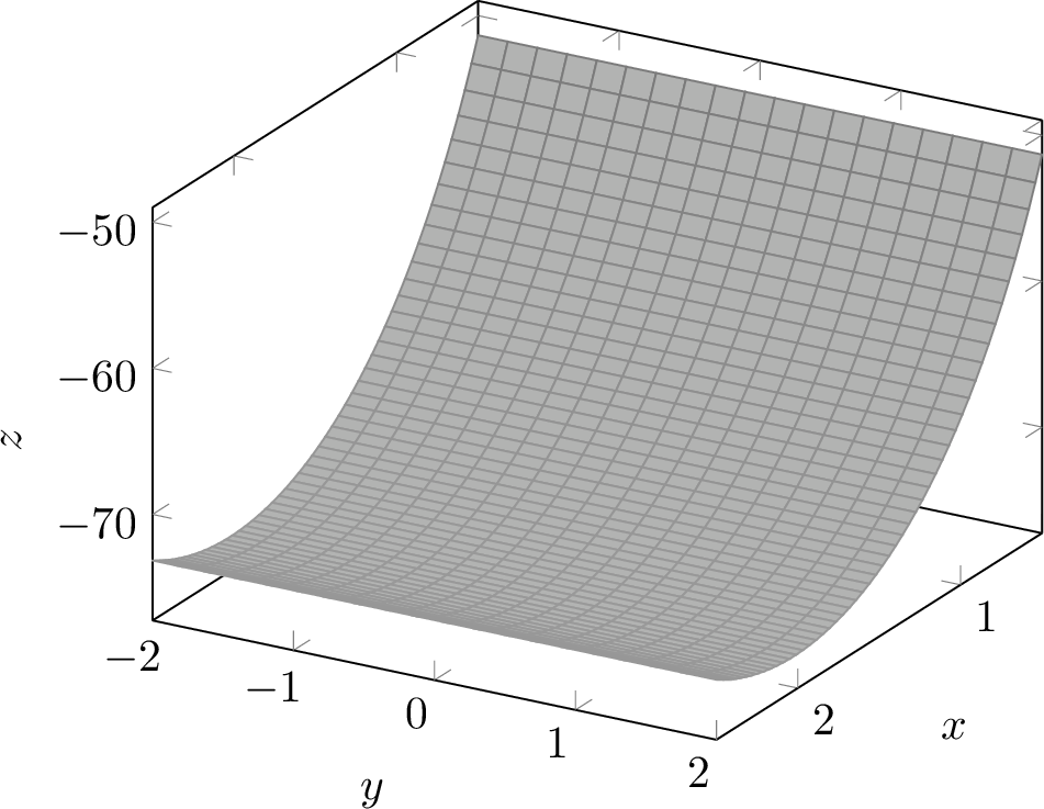
Theorem 2 illustrates how to obtain the surface mentioned in Figure 1.
3 Harmonic basis vector fields on surfaces of revolution↩︎
A surface of revolution is a surface \(M^2 \subset \mathbb{R}^3\) obtained by rotating a planar curve \(\Gamma\), called the generatrix, through a full revolution about a fixed axis of rotation \(\pi\), which in general does not intersect \(\Gamma\) except possibly at its endpoints. Let \(\Gamma\) be a curve defined by \[\Gamma : I \to \mathbb{R}^3, \qquad u \mapsto (f(u),0,h(u)),\] where \(I\) is an open interval of \(\mathbb{R}\) and \(f,h\) are smooth functions on \(I\) such that \(f'(u)\neq 0\) and \(h'(u)\neq 0\) for all \(u\in I\). By rotating the curve \(\Gamma\) about the \(z\)-axis, we obtain a surface of revolution \(M^2\) parametrized by \[\phi : I \times (0,2\pi) \to \mathbb{R}^3, \qquad (u,v) \mapsto \big(f(u)\sin v,\, f(u)\cos v,\, h(u)\big).\] The coordinate vector fields (basis vector fields) on the surface of revolution \(M^2\) associated with the above parametrization are given by \[\frac{\partial}{\partial u} = \big(f'(u)\sin v,\, f'(u)\cos v,\, h'(u)\big), \qquad \frac{\partial}{\partial v} = \big(f(u)\cos v,\,-f(u)\sin v,\, 0\big).\] We set \(\sigma(u)^2 = f'(u)^2 + h'(u)^2.\) Then the induced Riemannian metric \(g\) on the surface \(S\) is given, in the coordinates \((u,v)\), by \[g = \begin{pmatrix} \sigma(u)^2 & 0 \\[0.2cm] 0 & f(u)^2 \end{pmatrix}.\] We obtain the rough Laplacians of the coordinate vector fields as \[\begin{align} \Delta \left(\frac{\partial}{\partial u}\right) &= \left( \frac{\sigma''(u)\,\sigma(u) - \big(\sigma'(u)\big)^2}{\sigma(u)^4} - \frac{(f'(u))^2}{f(u)^2 \,\sigma(u)^2} + \frac{f'(u)\,\sigma'(u)}{f(u)\,\sigma(u)^3} \right) \frac{\partial}{\partial u}, \\ \Delta \left(\frac{\partial}{\partial v}\right) &= \left( \frac{f''(u)\,\sigma(u) - f'(u)\,\sigma'(u)}{f(u)\,\sigma(u)^3} \right) \frac{\partial}{\partial v}. \end{align}\] The vector fields \(\frac{\partial}{\partial u}\) and \(\frac{\partial}{\partial v}\) on the surface \(M^2\) are harmonic if and only if \[\begin{align} \label{1-1} \begin{cases} \dfrac{\sigma''(u)\,\sigma(u)-\big(\sigma'(u)\big)^{2}}{\sigma(u)^{4}} - \dfrac{(f'(u))^{2}}{f(u)^{2}\,\sigma(u)^{2}} + \dfrac{f'(u)\,\sigma'(u)}{f(u)\,\sigma(u)^{3}} = 0, \\[0.2cm] \dfrac{f''(u)\,\sigma(u) - f'(u)\,\sigma'(u)}{f(u)\,\sigma(u)^{3}} = 0. \end{cases} \end{align}\tag{19}\] Equivalently, multiplying through by appropriate powers of \(f(u)\) and \(\sigma(u)\), the above system can be rewritten as \[\begin{align} \tag{20} \big(\sigma''(u)\,\sigma(u)-\sigma'(u)^{2}\big) f(u)^{2} - (f'(u))^{2}\, \sigma(u)^{2} + f(u)\, \sigma(u)\, f'(u)\, \sigma'(u) &= 0, \\[0.2cm] \tag{21} f''(u)\,\sigma(u) - f'(u)\,\sigma'(u) &= 0. \end{align}\] Replacing \[\sigma'(u) = \frac{f'(u) f''(u) + h'(u) h''(u)}{\sqrt{f'(u)^2 + h'(u)^2}}\] into equation 21 , we obtain \[\begin{align} \label{1-4} h'(u) \big(f''(u)\,h'(u) - h''(u)\,f'(u)\big) = 0. \end{align}\tag{22}\]
Recall that the Gauss curvature \(K\) and the mean curvature \(H\) of a surface of revolution are given by \[\begin{align}
K &= \frac{h'(u)\,\big(f''(u)\,h'(u) - h''(u)\,f'(u)\big)}{f(u)\,\big(f'(u)^2 + h'(u)^2\big)^2}, \\
H &= \frac{-h'(u) + f(u)\,\big(h''(u)\,f'(u) - h'(u)\,f''(u)\big)}{2 f(u)}.
\end{align}\] Then equation 22 shows that the vector field \(\frac{\partial}{\partial v}\) is harmonic if and only if \(K = 0\). From \(K=0\), we obtain \[h'(u) = 0 \quad \text{or} \quad f''(u)\,h'(u) - h''(u)\,f'(u) = 0.\] In these cases, the mean curvature \(H\)
satisfies \[H = 0 \quad \text{or} \quad H = \frac{-h'(u)}{2 f(u)}.\] This implies that surfaces of revolution whose basis vector fields are harmonic necessarily have zero Gaussian curvature; in other words, such
surfaces are either planar or parabolic.
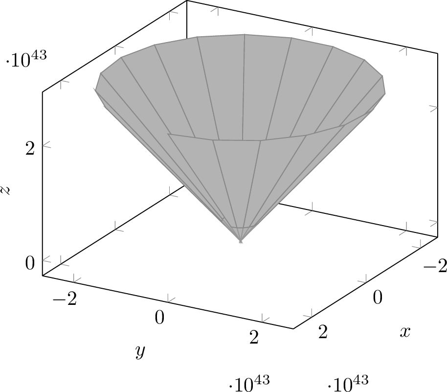
We illustrate how to obtain the surface mentioned above in Figure 2.
Theorem 3. A surface of revolution admits harmonic coordinate vector fields if and only if it is a plane, a cylinder, or a cone.
Proof. We recall that \[\sigma(u)^2 = f'(u)^2 + h'(u)^2.\] Case 1: Suppose \(\sigma = c\), where \(c\) is a positive
real constant. Then \[h'(u) = \pm \sqrt{c^2 - f'(u)^2}, \quad \text{with } f'(u)^2 \leq c^2.\] In this case, formula (19 ) becomes \[\begin{align}
\begin{cases}
\Delta\Big(\dfrac{\partial}{\partial u}\Big) = \dfrac{-f'(u)^2}{c^2 f(u)^2} \dfrac{\partial}{\partial u},\\[2mm]
\Delta\Big(\dfrac{\partial}{\partial v}\Big) = \dfrac{f''(u)}{c^2 f(u)} \dfrac{\partial}{\partial v}.
\end{cases}
\end{align}\] In the case \(f'(u) = 0\), i.e., \(f(u) = c \neq 0\), we have \[h'(u) = \sqrt{c^2 - a^2}, \quad \text{so} \quad h(u) = u \sqrt{c^2 -
a^2}.\] Then, the curve is parametrized by \[(c, 0, u \sqrt{c^2 - a^2}), \quad \text{with } a, c \in \mathbb{R}_+^* \text{ and } a^2 < c^2.\] Consequently, the surface generated is parametrized as \[\phi(u,v) = \big(a \cos v, \; a \sin v, \; u \sqrt{c^2 - a^2}\big),\] which is a cylinder of revolution defined by the equation \[x^2 + y^2 = a^2.\] Case 2: If \(h'(u) = 0\), then \(h\) is constant. Let us take \(h(u) = a\), with \(a \in \mathbb{R}_+\). In this case, we have \(\sigma(u) = \pm f'(u)\). The vector field \(\frac{\partial}{\partial v}\) is harmonic and \[\Delta\Big(\frac{\partial}{\partial u}\Big) =
\frac{f^2 f' f''' - f^2 (f'')^2 - (f')^4 + f (f')^2 f''}{f^2 (f')^4} \, \frac{\partial}{\partial u}.\] Thus, the vector field \(\frac{\partial}{\partial u}\) is harmonic if
and only if \[\label{2-1}
f^2 f' f''' - f^2 (f'')^2 - (f')^4 + f (f')^2 f'' = 0.\tag{23}\] Thus, we have \[f(u) = \sqrt{k e^{\alpha u} + \beta}, \quad
k \in \mathbb{R}^*, \;\; \beta \in \mathbb{R}_+, \;\; \text{with } \beta + k e^{\alpha u} > 0.\] In this case, the surface is parametrized by \[\phi(u,v)
= \big(\sqrt{k e^{\alpha u} + \beta} \cos v, \; \sqrt{k e^{\alpha u} + \beta} \sin v, \; a\big),\] where \(a \in \mathbb{R}_+, \;\; k \in \mathbb{R}^*, \;\; \beta \in \mathbb{R}_+, \;\; \text{with } \beta + k e^{\alpha u}
> 0.\) Therefore, the surface of revolution is the plane defined by the equation \(z = a.\)
Case 3: If \(h' \neq 0\) and \(f'' h' - h'' f' = 0\) (\(K = 0\)), then the surface is of parabolic type. We
distinguish two subcases.
Case 3.1: If \(f' = 0\). Suppose \(f(u) = a \neq 0\), then \(\sigma(u) = \pm h'(u)\). We have \[\Delta\Big(\frac{\partial}{\partial v}\Big) = 0,\] but \[\Delta\Big(\frac{\partial}{\partial u}\Big) = 0 \quad \text{if} \quad
\frac{\sigma'' \sigma - (\sigma')^2}{\sigma^4} - \frac{(f')^2}{f^2 \sigma^2} + \frac{f' \sigma'}{f \sigma^3} = 0.\] This is equivalent to \[\frac{(\sigma''
\sigma - (\sigma')^2) f^2 - (f')^2 \sigma^2 + f \sigma f f' \sigma}{f^2 \sigma^4} = 0
\quad \Longleftrightarrow \quad
\frac{h''' h' - (h'')^2}{(h')^2} = 0. \label{2-2}\tag{24}\] Therefore, the basis vector fields are harmonic if and only if \[h''' h' - (h'')^2 = 0.\] We now
discuss two subcases for the third case.
Case 3.1.1: If \(h'' = 0\). In this situation, the condition \[h''' h' - (h'')^2 = 0\] is automatically satisfied, which implies \[\Delta\Big(\frac{\partial}{\partial u}\Big) = 0.\]
Thus, the basis vector fields are harmonic if \[f(u) = a, \quad h(u) = b u + c, \quad \text{where } a, b \in \mathbb{R}^*, \; c \in \mathbb{R}.\]
The corresponding surface is parametrized by \[\phi(u,v) = (a \cos v, \; a \sin v, \; b u + c), \quad a, b \in \mathbb{R}_+^*, \; c \in \mathbb{R}.\]
Hence, the surface is a cylinder of revolution defined by the equation \[x^2 + y^2 = a^2, \quad a \in \mathbb{R}_+^*.\]
Case 3.1.2: If \(h'' \neq 0\). From equation (24 ), we have \(\frac{h'''}{h''} = \frac{h''}{h'}\). So that \(h(u) = \frac{b}{a} e^{a u} + c,\) where \(a, b \in \mathbb{R}^*, \; c \in \mathbb{R}.\) The basis vector fields are harmonic if \[f(u) = a, \quad h(u) = \frac{b}{a} e^{a u} + c, \quad a, b \in \mathbb{R}^*, \; c \in \mathbb{R}.\] Hence, the surface is parametrized by \[\phi(u,v) = \Big(a \cos v, \; a \sin v, \; \frac{b}{a} e^{a u} + c \Big), \quad a, b \in \mathbb{R}_+^*, \; c \in \mathbb{R}.\]
Moreover, the surface is a surface of revolution, namely a cylinder defined by \[x^{2}+y^{2}=a^{2}, \qquad a\in \mathbb{R}_{+}^{42}.\]
Case 3.2: Assume that \({f'\neq 0}\). Then we have \[\begin{align} f''h'-h''f' = 0 &\;\Longleftrightarrow\; \frac{f''}{f'}=\frac{h''}{h'} \\ &\;\Longleftrightarrow\; \ln |f'|=\ln |h'| \\ &\;\Longleftrightarrow\; f'=a\,h', \qquad a\in\mathbb{R}^{42} \\ &\;\Longleftrightarrow\; f(u)=a\,h(u)+b, \qquad a\in\mathbb{R}^{42},\; b\in\mathbb{R}. \end{align}\]
Furthermore, \[\begin{align} \sigma^{2}=f'^{2}+h'^{2} &\;\Longrightarrow\; \sigma^{2}=(1+a^{2})\,f'^{2} \\ &\;\Longrightarrow\; \sigma=\pm\sqrt{1+a^{2}}\,f'. \end{align}\]
In this case, we obtain \[\begin{align} \begin{cases} \displaystyle \Delta\!\left(\frac{\partial}{\partial u}\right) =\left( \frac{\sigma''\sigma-\sigma'^{2}}{\sigma^{4}} -\frac{f'^{2}}{f^{2}\sigma^{2}} +\frac{f'\sigma'}{f\sigma^{3}} \right)\frac{\partial}{\partial u}, \\[1em] \displaystyle \Delta\!\left(\frac{\partial}{\partial v}\right)=0, \end{cases} \end{align}\] which is equivalent to \[\begin{align} \begin{cases} \displaystyle \Delta\!\left(\frac{\partial}{\partial u}\right) =\frac{(\sigma''\sigma-\sigma'^{2})f^{2} -f'^{2}\sigma^{2} +f\sigma f'\sigma'}{f^{2}\sigma^{4}} \frac{\partial}{\partial u}, \\[1em] \displaystyle \Delta\!\left(\frac{\partial}{\partial v}\right)=0, \end{cases} \end{align}\] and hence \[\begin{align} \begin{cases} \displaystyle \Delta\!\left(\frac{\partial}{\partial u}\right) =\frac{1}{a} \frac{ h^{2}h'h'''-h^{2}h''^{2}-h'^{4}+hh'^{2}h'' }{ h^{2}h'^{4} } \frac{\partial}{\partial u}, \\[1em] \displaystyle \Delta\!\left(\frac{\partial}{\partial v}\right)=0. \end{cases} \end{align}\] We obtain that the coordinate vector fields are harmonic if \[f(u)=a\,h(u)+b, \qquad a\in\mathbb{R}^{42}, \; b\in\mathbb{R}.\]
Moreover, the function \(h\) satisfies equation 23 with \(h'\neq 0\), namely \[h^{2}h'h'''-h^{2}h''^{2}-h'^{4}+h h'^{2}h''=0.\] Solving this differential equation yields \[\begin{cases} h(u)=\sqrt{k e^{\alpha u}+\beta},\\[0.5em] f(u)=a\sqrt{k e^{\alpha u}+\beta}+b, \end{cases}\] where \[a,k\in\mathbb{R}^{42}, \qquad b,\beta\in\mathbb{R}, \qquad \text{with } \beta+k e^{\alpha u}>0.\]
Hence, the surface is parametrized by \[\begin{align} \phi(u,v) &=\bigl((a h(u)+b)\cos v,\,(a h(u)+b)\sin v,\,h(u)\bigr)\\ &=\Bigl(\bigl(a\sqrt{k e^{\alpha u}+\beta}+b\bigr)\cos v,\, \bigl(a\sqrt{k e^{\alpha u}+\beta}+b\bigr)\sin v,\, \sqrt{k e^{\alpha u}+\beta}\Bigr). \end{align}\]
Therefore, the surface is a cone parametrized by \(\phi\). Its Gaussian curvature and mean curvature are given by \[K=0, \qquad H=\frac{\alpha k e^{\alpha u}}{2\sqrt{k e^{\alpha u}+\beta}}\neq 0.\] ◻
Conflict of interest↩︎
The authors declare no conflict of interest.
Data Availability↩︎
Not applicable.